BUTP-2002/03
LU TP 02-05
February 2002
Eta decays at and beyond in Chiral Perturbation
Theory111Talks presented at the Workshop on Eta Physics,
Ångström laboratory, Uppsala, October 25-27, 2001; published in the
proceedings (Physica Scripta Topical Issues T99 (2002) 34).
Johan Bijnensa and Jürg Gasserb
aDepartment of Theoretical Physics, Lund University
Sölvegatan 14A, S-22362 Lund, Sweden
bInstitute of Theoretical Physics, University of Bern
Sidlerstrasse 5, CH-3012 Bern, Switzerland
PACS: 12.39.Fe (Chiral Lagrangians),
13.40.Hq (Electromagnetic decays),
14.40.Aq (pi , K, and eta mesons),
12.15.Ff (Quark and lepton masses and mixing)
An overview is given of Chiral Perturbation Theory and various applications to eta decays. In particular, the main decay is discussed at the one-loop level, and estimates of the higher order corrections are given. The importance of and higher order effects in double Dalitz and decays is pointed out. In all these cases the need for new experimental results is stressed.
1 Introduction
Eta decays at high precision, both in measuring rare decays and in precisely determining kinematical distributions in the more common decays, have a high potential to teach us about various aspects of the strong interaction. In the view of the new experimental results to be expected from WASA at CELSIUS in Uppsala and KLOE at DAPHNE in Frascati and the ongoing work of the Crystal Ball, an overview of the present situation as regards some of the main eta decays is appropriate. The importance of these decays and measurements can be judged from the fact that they were the main focus of several theoretical talks presented at this workshop, in addition to the ones by the present authors there is also the contribution by Holstein[1] and by Ametller[2].
In this review we concentrate on chiral symmetry aspects for the main strong decay and how it can be used to extract information on quark mass ratios. We will show how precise measurements of the slope parameters will lead to more refined theoretical predictions for the decay rate as a function of the quark mass ratio
| (1) |
A discussion of the decay in Chiral Perturbation Theory (CHPT) and the use of dispersion theory to improve on the one-loop prediction is the main focus of this short review. In addition, a short overview is given of Dalitz () and double Dalitz () decays, as well as of the process . We indicate why these are important quantities to be measured.
We first give a very short overview of chiral symmetry and its incorporation using effective field theory methods - known as Chiral Perturbation Theory - in Sect. 2. The decay is then discussed at the purely perturbative level in CHPT at order in Sect. 3 and the estimates of higher orders using dispersion relations in Sect. 4. Section 5 is devoted to the Dalitz and double Dalitz decays, and the decay is the subject of section 6. Our conclusions are presented in section 7.
2 Basics of CHPT
We cannot calculate all things we are interested in in the strong interaction directly from QCD. E.g. scattering amplitudes at low energies cannot be expressed as an expansion in the strong coupling constant because:
-
•
At low energies the coupling constant becomes large.
-
•
We deal with bound states which require always to go beyond a simple perturbation series.
So how can we calculate e.g. the cross-section of -scattering in QCD?
Two fundamental options are possible:
- Lattice:
-
This can be done using the methods developed by Lüscher[3] via QCD calculations at finite volume. The energy spectrum at finite volume depends on the interaction. By measuring the lowest two-pion energy level, the wave scattering lengths can be obtained via
(2) where denotes isospin. There are first lattice results available which make use of this relation [4].
- Effective Theory of QCD:
-
Using the methods of effective quantum field theory (EFT) we can also evaluate cross-sections in QCD at low energies. We replace the QCD Lagrangian by the effective Lagrangian of Chiral Perturbation Theory (CHPT). We replace the quarks and gluons by the degrees of freedom which are relevant at low energies: , , , , ,…. This is the method most of this report is concerned with.
Chiral Perturbation Theory does reproduce for appropriately chosen coupling constants the -matrix elements of QCD[5] and it allows to make very sharp predictions in some cases. As an example, we quote the recent result on the scattering length combination [6],
| (3) |
For earlier work at tree level and at one and two-loops accuracy, see [7, 8, 9].
We will now present the basics which underly the calculations of , , etc. in this approach.
2.1 Chiral Symmetry
Consider QCD with 3 flavours, , and . Gluon interactions do not change the helicity of a quark, only mass terms couple the left and right handed helicity states. So in the limit where , the left-handed world cannot be turned into the right handed world. Now if all the masses are zero, there is also no way to distinguish the different flavours of quarks and we can continuously rotate one into the other. The QCD Lagrangian is thus invariant under
| (4) |
separately for both helicities, left (L) and right (R). The matrices are general unitary matrices. So we have a global222The parts of the groups play no role here, but see the contributions by Bass[10], Shore[11], Michael[12], Kroll and Feldmann[13] for their effects.
| (5) |
chiral symmetry of QCD . This symmetry has 16 conserved currents and has thus 16 conserved charges. The vector charges also annihilate the vacuum, but the axial charges produce a change on the vacuum:
| (6) |
The symmetry of the QCD Lagrangian is not the symmetry of the vacuum. This is known as spontaneous breakdown of chiral symmetry or spontaneous chiral symmetry breaking ((S)SB).
The 8 spontaneously broken axial symmetries require the existence of 8 Goldstone bosons which must be massless and pseudoscalar. They are the pions, kaons and eta. The Goldstone bosons also have zero interactions at zero energy. The expansion of CHPT is based on these facts.
Now, the fact that the quark masses are present and we can also have nonzero energies allows nonzero values for masses and interactions. E.g. the pion mass is an intricate mixture of the current quark mass, explicit SB, and the quark vacuum expectation value, spontaneous SB[14].
| (7) |
Similarly the pion scattering lengths do not vanish[7]
| (8) |
These predictions are not exact, they are the first term in a series expansion of momenta and the quark masses.
2.2 A systematic expansion
The amplitudes are expanded in powers of momenta and quark masses. The price paid for the generality is that order by order we get more terms,
| (9) |
where contains terms with -derivatives or equivalent. In amplitudes the derivatives turn into momenta such that the expansion converges at low momenta. As said earlier, quark masses are counted as two powers of momentum, this is because Eq. (7) sets a quark mass to the pion mass squared. The structure of the Lagrangians is fixed by chiral symmetry but the coupling constants are not.
In the strong and semileptonic mesonic sector, these Lagrangians are known and the parameters have conventional names:
These coupling constants (LEC’s) are free in chiral perturbation theory, but are in principle calculable from QCD333For some attempts to determine them from lattice QCD, see Ref. [18]..
The Lagrangians allow to calculate S-matrix elements order by order in powers of momenta and quark masses. The main point is that order by order, only a limited number of terms can contribute, and the form of the contribution is completely fixed by chiral symmetry. So an amplitude can be expanded in powers
| (10) |
with
- :
-
tree graphs with vertices from . The form of the vertices is fixed by chiral symmetry.
- :
-
tree graphs with vertices from and one vertex from or loop graphs with vertices from .
This procedure is known as Chiral Perturbation Theory (CHPT).
In loop integrals one integrates over all momenta, from eV to the Planck mass and beyond, yet we always use the vertices from the effective Lagrangian constructed to reproduce the amplitude at low energies. This is not a contradiction, the high energy behaviour of the loop integrals is irrelevant in the sense that this is the part that is absorbed by the coupling constants. In this way, different regularizations can be used to cut-off the integrals and the difference in different ways of doing it is absorbed by using different values of the coupling constants. The final result is always independent of the regularization used. In practice we nearly always use dimensional regularization since it preserves chiral symmetry throughout the calculation reducing the need for technically complicated subtractions to restore symmetries.
3 at order
3.1 Kinematics and Isospin Relations
The is an isospin singlet and a pseudo-scalar. The decay into two pions is forbidden by CP. CP violation in decays is discussed by C. Jarlskog and E. Shabalin[21] and J. Ng[22] in these proceedings. Three pions in an angular momentum 0 configuration cannot have isospin zero as well, but isospin 1 is allowed. This decay thus has to proceed via isospin breaking effects. Electromagnetism is known to play a fairly minor role here as discussed below, except via the kinematical effects due to the charged and neutral pion mass difference. This decay thus goes primarily through the strong isospin breaking part of QCD
| (11) |
This itself has isospin 1 and there is thus to lowest order in isospin breaking a relation between and .
The kinematics is depicted in Fig. 1.
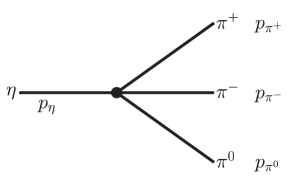
The variables used in the remainder are
| (12) |
which satisfy
| (13) |
The last equality is the definition of .
The decay amplitude itself can be written as
| (14) |
Charge conjugation requires this amplitude to be symmetric under the interchange of and so we have
| (15) |
Using isospin as discussed above and labeling the three momenta as and , the amplitude for the neutral decay
| (16) |
satisfies
| (17) |
see e.g. [23] for a detailed derivation of this result. Experimentally, there are two main numbers to be kept in mind[24]. The decay width from an overall fit
| (18) |
with a scale factor of , and the ratio of neutral to charged decays
| (19) |
with a scale factor of . The presence of these scale factors is an indication of mutually incompatible experiments.
3.2 Lowest order:
The lowest order CHPT contribution from the quark mass difference was derived in the sixties using current algebra methods[25] and is
| (20) |
As announced, the decay amplitude is proportional to . We can now rewrite the amplitude in terms of , a combination of quark masses which is experimentally more easily accessible,
| (21) |
where stands for the up, down or strange current quark mass, and
| (22) |
The decay rate can then be written as
| (23) |
with at lowest order
| (24) |
It can alternatively be rewritten in terms of
| (25) |
as
| (26) |
So if we have a good theoretical description of , we get an accurate determination of , since
| (27) |
Due to the high power, the error on can be made much smaller than its determination from meson mass ratios,
| (28) |
because this relation has much larger electromagnetic corrections[26].
In order to show the accuracy which can be obtained, we can input two different values of or . We first use the value
| (29) |
The second one is where we use instead the fit done at order for the quark masses from the meson masses and the estimate of the kaon electromagnetic mass difference including higher order effects [28],
| (30) |
It is clear that a good understanding of can lead to a very accurate determination of and .
3.3 Electromagnetic effects
The lowest order contribution does not contribute directly to the decay rate. It only comes in via the electromagnetic mass difference of pions. This is very relevant for the actual values of the kinematical variables in terms of the measured momenta, but this can be included in a simple fashion. That this decay could not be explained by its electromagnetic contributions has been known for a long time already[29].
The calculation of the purely electromagnetic contribution to the decay has also been pushed to one-loop level[30] and the total effect remains small.
The decay with an extra photon in the final state has been estimated as well. This could have had potentially a large impact, since it can proceed without extra isospin breaking. Fortunately, both a simplified analysis using Low’s theorem[31] and a full analysis at one loop in CHPT[32] lead to a rather small result of the order of 1% of the decay width of .
The correct incorporation of the electromagnetic corrections also tells us which value for the pion mass should be introduced in the expression for the amplitude. It is the same for both decays and is the neutral pion mass but we need to include the correct physical masses in the phase-space integrals. This follows from adding to the effective electromagnetic term
| (31) |
with
| (32) |
There is no direct contribution to . The first term leads to an equal mass shift for the charged pion and charged kaon in the chiral limit. This fact is known as Dashen’s theorem[33]. The second term generates a contribution through mixing. This may appear to be negligibly small, because it is of order . However, this matters in the ratio . Taking these corrections into account tells us that the pion mass appearing in Eq. (26) is the neutral pion mass.
3.4 Conclusions from the tree level
-
•
The total rate is off by a factor of about 4, depending on the precise inputs used.
-
•
The ratio is near its experimental value. The reason for this is discussed below.
-
•
Second order isospin breaking effects are important in the phase-space. Since the latter is small, small terms are important there - they significantly lower .
-
•
The effective Lagrangian method is a very efficient tool to perform these calculations.
3.5 One-loop contribution
The amplitude can be expanded as
| (33) |
has been calculated in the previous subsections. To evaluate , one needs to evaluate one-loop diagrams with and tree diagrams with . This was done in Ref. [34]. The decay rate can now be written in the form of Eq. (23). From the expression in Ref. [34], it can be seen that the only free parameter coming in is . This parameter can be determined from -scattering[16] or more accurately from decays[28, 35].
What one numerically finds is a very large enhancement over the lowest order expression,
| (34) |
where stands for Lorentz invariant phase-space. This enhancement has as one major source the large -wave final state rescattering as was expected, see Ref. [36] and references therein. In Sect. 4 we will come back to estimates of this contribution to higher orders. This contributions is about half of the total enhancement found in Ref. [34].
3.6 and slope parameters
Can be very different from 1.5? The lowest order amplitude has a zero for . Higher order corrections are not expected to remove the zero and also not to move it very much. We can thus expect that the amplitude will remain roughly of the form
| (35) |
with about 4/3. Given this form we see from Fig. 2 that unless the zero moves very much, the ratio will remain close to 1.5.
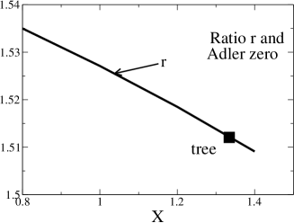
The reason for this relation between and the ratio is the isospin relation between the amplitudes for the neutral and charged decays.
At the ratio is changed from the tree level prediction. It is now lowered to 1.43, bringing it into nice agreement with the observed ratio. Again, the relation between , or more generally the slope measurements in the Dalitz plot, and follows from isospin. This is discussed in detail in Ref. [34].
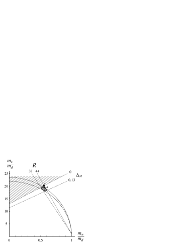
3.7 at order
The quark mass ratio determines the major semi axis of Leutwyler’s ellipse in the and plane[27],
| (36) |
The situation at order is shown in Fig. 3.
The role that a better understanding of has in this context is shown in Fig. 4,
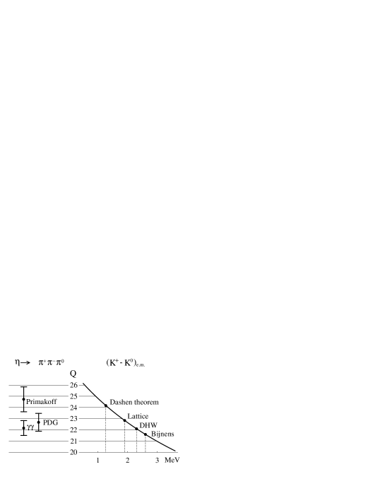
where at order the measurement of is compared with the determination from the - mass difference. The different points on the graph correspond to various estimates of the electromagnetic part of the mass difference. Note that estimates of the contributions [28] indicate possibly even lower values of than are shown here.
4 beyond order
4.1 The method and equations to solve
We can now try to estimate even higher orders using dispersion relation techniques. This should catch a large part of the higher order corrections, because the large rescattering part was already a large part of the one-loop prediction. Unfortunately, for a general three-body decay, this is not such an easy undertaking. There are several subtleties involved here, as compared to the simple case of a two-body final state, because one can have imaginary parts not only from the scattering, but also from the unstable particle. The latter difficulty can be avoided by studying instead the scattering process with an mass such that the eta cannot decay. Then we only have singularities in the various channels to deal with. This procedure is how one can restrict oneself to the influence of two-body scattering only. The general framework is known as Khuri-Treiman equations [37] and was used in Ref. [38] to study higher order corrections to eta decay.
Here we will restrict ourselves to a simpler formalism that has been very successful in the study of scattering[39]. The underlying observation is that there are no imaginary parts from rescattering with angular momentum larger than or equal to two up to . This together with the fact that is constant shows that to order the amplitude (23) can be written as
| (37) |
The functions correspond to isospin rescattering in the two particles whose kinematics is described by . The split into these functions is not quite unique. There is some ambiguity in the distribution of the polynomial terms over the various , because is constant. The split (37) is useful because:
-
•
Dispersion problems are now reduced to a set of functions of only one variable much simplifying the analysis.
-
•
This split is fully correct to two-loop order.
-
•
The main two-body rescattering corrections happen inside the functions .
This method was used to estimate higher order corrections to in Ref. [40]. A detailed description can be found in Ref. [23]. With the approximations used in Ref. [38], the two methods are in fact entirely equivalent.
So we use here the form (23) and discuss the process with the final two pions in isospin for an eta mass below the three pion threshold. This leads to the dispersion relations
| (38) |
up to subtractions, see below. To be more precise, the integrand contains the discontinuity
| (39) |
We will need to subtract to be able to compare with the one-loop expression. Checking the high-energy behaviour of the one-loop expressions leads to three subtractions for and , while two are sufficient for . So the equations we will need to solve for are
| (40) |
This leads to eight constants which should be determined. But the ambiguity in the precise choice of the is visible here too. Up to the same order in the expansion we have only four parameters
| (41) |
so there is some freedom in the choice.
We can form some more convergent combinations at one-loop as well. Comparing expressions one sees that
| (42) |
and
| (43) |
need only two subtractions. This allows to determine and in terms of and integrals over the discontinuities via
| (44) |
So once we know , and , this forms a set of integral equations that can be solved. Now we have to put in the knowledge of the phases. In a single channel problem without singularities in the cross channel, this problem is simple and was solved by Omnès long ago. Here we have cross-channel singularities but they are again scattering in an isospin 0,1,2 state. The discontinuities thus obey[41]
| (45) |
with a consequence of the singularities in the and channel. They satisfy
| (46) |
where is the appropriate for a scattering of angle with center of mass energy squared of . The coefficients can be found in [23, 41].
So at least we have a principle solution. There are several technical complications involved. After analytically continuing to its physical value, extra singularities appear, and we need for values of outside the physical domain, so singularities in the relation of with and appear. The integration path needs to be chosen carefully to avoid these extra singularities. Having solved this problem, one finds that the solution to the equations is not unique. The problem is that homogeneous equations of the type
| (47) |
have nontrivial solutions - we need to pick out the physically correct one. The solution is [40] to write a dispersion relation for a related function which only has one solution. We remove the singularity in the direct channel by dispersing instead
| (48) |
with
| (49) |
Similar arguments to above lead then to the dispersion relations with a total of 4 subtraction constants for the . They are, rewritten in the ,
| (50) |
So basically we now have to find a parametrization of , the phaseshifts, and determine the subtraction constants. After that the above equations can be solved numerically. Two of the constants can be determined similarly to and above, leading to
| (51) |
The values of these two parameters compared with the one-loop expressions are basically independent of the matching points. The other two are discussed in the next section.
4.2 Results
The two papers [40] and [38] basically only differ in the choice of the subtraction procedure. As explained above, the formalism is quite different but the underlying approximations and assumptions are the same.
Reference [40] looks at the lowest order expression for
| (52) |
and notices that we can determine and from the place of the zero, the Adler zero happening at , and the value of the slope in at .
Reference [38] instead uses several values of to fit the dispersive approximation to the one-loop result. The resulting divergence in results is taken as an estimate of the theoretical error. The final result for the enhancement over the one-loop result is quite similar in both papers, but a closer look at the intermediate results shows some discrepancies which need to be understood. The one thing which can be compared are the published plots of as a function of along the line . These are shown in Fig. 5 and 6.
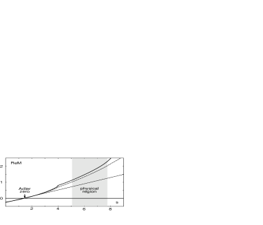

Notice that while both have a significant enhancement, the slope is quite different. The results of [40] are always above the one-loop result while the results of [38] cross the one-loop result at the end of the physical region. Given the similarity of the methods and the inputs used, this type of discrepancies needs to be understood, but it is obvious that a better experimental determination of the slopes can distinguish between both calculations. It is therefore very important that all slope parameters, see below for the definitions, are well measured.
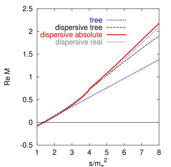
As a simple estimate of the uncertainties involved, we have used a simplified version of the equations (4.1) where we set the functions . So we only consider rescattering effects in the direct channel. We then fix the values of and , considered real, to the tree level slope and Adler zero. In Fig. 7 the tree level is shown (tree) and the dispersive improved tree level (dispersive tree). The two dispersive improvements of the one-loop result shown are using the position of the one-loop Adler zero, and either the absolute value of the slope (dispersive absolute) or its real part (dispersive real) at one-loop to determine and . It can be seen that these predictions lead to different slopes in the physical regions, thus allowing the theoretical subtraction procedure to be experimentally tested. Notice that we have shown only one variation in the phase-space. The variation over all of phase-space can of course be used similarly.
4.3 Dalitz plot expansions or slope parameters
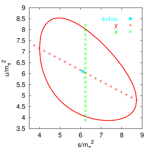
Once the amplitude is known, one can easily expand the Dalitz plot distributions around the center of the Dalitz plot. Notice that some care is needed to precisely define the center of the Dalitz plot, given the second order isospin breakings discussed earlier. The point does not quite coincide with the point where all kinetic energies are equal for the charged decay. The usual definition of the slope parameters is in terms of the kinematical variables and ,
| (53) |
stands for the kinetic energy of the pion of charge . In Fig. 8 we have shown how and depend on and . The crosses correspond to and equal to , ,…,. The correspond to and . The filled square indicates the place where . The difference with the point is again an indication of the isospin breaking effects in the masses discussed earlier.
The measured distribution is now parametrized as follows. For the charged decay, one takes
| (54) |
normalized to the center of the Dalitz plot, and
| (55) |
for the neutral decay. It is hard to compare with the experimental results in the review of particle properties [24]. They simply state that the assumptions made in the different measurements are not compatible. The problem is that making assumptions on the values of the quadratic slopes significantly alters the fitted result of the others. In table 1 we show the theoretical results of tree level, one-loop, the dispersive results from [38] and the results of the tree dispersive and absolute dispersive simplified estimates discussed above. Note that the one-loop predictions of the neutral slope is not zero, contrary to the statement made in Refs. [42, 48]. The loops themselves do give a contribution, whereas the contributions from the tree and tadpole diagrams at happen to vanish. The precise value is dependent on the procedure used and is sensitive to fairly small changes. The number quoted corresponds to the precise way the expressions are given in [34]. We plan to come back to this issue in a later publication.
| tree | 0.25 | 0.00 | ||
|---|---|---|---|---|
| one-loop [34] | 0.42 | 0.08 | 0.03a | |
| dispersive [38] | 0.26 | 0.10 | — | |
| tree dispersive | 0.31 | 0.001 | ||
| absolute dispersive | 0.33 | 0.04 |
Measurements as mentioned earlier are difficult to compare, but several new results have been obtained recently. In particular, the new Crystal Ball value for was announced at this meeting [49]. Note that the experiments usually quote . For completeness the known experimental results are given in table 2 for the charged decay and table 3 for the neutral decay.
| Layter[43] | |||
|---|---|---|---|
| Gormley[44] | |||
| Crystal Barrel[45] | |||
| Crystal Barrel[46] | 0.06 fixed |
| Alde[47] | |
|---|---|
| Crystal Barrel[48] | |
| Crystal Ball[49, 42] |
Notice that while the overall agreement is all right, there is a problem in obtaining a value of which is compatible with the newer experiments. The theoretical evaluation of suffers from large cancellations.
5 Dalitz and double Dalitz decays
This section is a shortened version of the work presented in Ref. [50]. The underlying question is how well do we understand the couplings of the to two photons. In table 4 we show the (expected) branching ratios for all of the decays with two photons. The decays with one lepton-antilepton pair are known as Dalitz decays, those with two pairs as double Dalitz decays.
| Decay | Branching ratio |
|---|---|
These decays allow us to study the off-shell structure of the vertex as shown in Fig. 9.
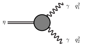
The question is: how does this form-factor behave over the entire range of off-shell masses for the photons? Is it of order 1, w.r.t. to on-shell photons, can it be described by adding vector meson propagators in the photon legs? One would also like to know the approach to the perturbative QCD result (see e.g. Ref. [51])
| (56) |
This type of form-factors are one of the places where experiments are possible for the same underlying physical process over the entire regime, ranging from the fully perturbative to the fully nonperturbative one. The large and intermediate values of and can be studied in tagged photon-photon collisions while the small timelike values can be studied in -decays.
To study how well -decays can see variations in the form-factor, in Ref. [50] four trial form-factors were investigated,
| (57) | |||||
| (58) | |||||
| (59) | |||||
| (60) |
The first form is included to check how well a deviation from a pointlike eta can actually be measured. The second one is the standard double vector meson dominance model, while the third was a variation that reproduced single vector meson dominance, while numerically approaching Eq. (56) quite well. The last form was suggested in Ref. [52], see also Ref. [53], Knecht and Nyffeler in Ref. [54] as well as the contribution by Feldmann and Kroll to this conference[13]. One important reason why we like to know this form-factor better is that pseudoscalar exchange is the major contribution to the hadronic light-by-light scattering part of the muon anomalous magnetic moment as studied in Ref. [54]. The contribution of the exchange of , and using the different form-factors to is [50, 54] for form-factor (58), for (59) and for (60). It is thus clearly important for future measurements of that this form-factor becomes experimentally more constrained.
In tables 5 to 7 we show the results [50] for the various decays as a function of the electron-positron mass lower bound as well the muonic cases for all of phase-space.
| Decay | (57) | (58),(59) | (60) | |
|---|---|---|---|---|
| 50 MeV | ||||
| 200 MeV | ||||
| 300 MeV | ||||
| 400 MeV | ||||
| — |
| Decay | (58) | (59) | (60) | |
|---|---|---|---|---|
| 50 MeV | ||||
| 200 MeV | ||||
| 300 MeV |
| Decay | (58) | (59) | (60) | |
|---|---|---|---|---|
| 50 MeV | ||||
| 100 MeV | ||||
| 200 MeV | ||||
| — |
It turns out that it is surprisingly difficult to see the difference between the various models of the form-factors in decays, but some constraints are possible. The form-factors which are different in single Dalitz decays should be easily distinguishable, but more subtle differences, as the one between (58) and (59) - which only become visible in double Dalitz decays - will be difficult to see. Given the importance of these results, the measurements should be performed. The differences between the effects of the the form-factors in (57) to (60) is . Form-factors (58) (59) only differ at . The differences are a good indication of the importance of the various orders.
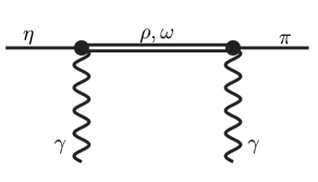
6
This decay is only touched upon in this report. A more comprehensive discussion can be found in the review by Ametller[2] and in the references. The main theory paper underlying this decay is [55], and the main interest is that this decay is a window on rather high order corrections in CHPT. The result is small for several reasons. The amplitude has two possible Lorentz structures. In the gauge , with and the polarization vector and momentum of photon , the amplitude can be written as
| (61) |
At only the part of the amplitude is nonzero and it is small. The pion loop is suppressed by isospin breaking and the kaon loop is suppressed by and an extra factor of in the integral. The contributions are
| sum | (62) |
rather far from the old experimental value of eV[24]. Newer experimental limits come from Novosibirsk[56] and the Crystal Ball[49]. The latter gives eV. The result of Eq. (6) is therefore more than two orders of magnitudes below the measured width.
We can also add vector meson exchange as depicted in Fig. 10. This starts at and has contributions to all orders. Restricting the exchange of and to terms only leads to eV and if all orders are kept
| (63) |
much larger than the suppressed contributions. In fact, there is one more contribution with well determined signs which appears at . Here there is no isospin suppression of the pion-loops any longer nor any factors like the at . As a result the contribution from the double WZW vertex one-loop diagram is as large as the one. Given the structure of the amplitude, interference effects are quite strong so that if we put in the loops plus the VMD estimates we obtain the estimate[55]
| (64) |
We can now add the contribution from and exchange, the absolute values are experimentally known but the signs are free. This leads to
| (65) |
in very nice agreement with the preliminary Crystal Ball result. Studies of distributions in the decays will allow to disentangle various contributions to this decay. It should be noted that studies of this decay mode have also been performed in the ENJL model[57] and by adding other resonances than the ones referred to above[58]. There also exist some recent quark model studies[59].
7 Conclusions
We have discussed several eta decays from the point of view of Chiral Perturbation Theory and various possible enhancements. The main conclusion is that more and precise measurements are very much needed.
This decay has the potential to deliver accurate quark mass ratios. For this we need better measurements of the slope parameters in the Dalitz plot and a better determination of the ratio between the neutral and charged decay mode. These will allow to put the theoretical calculations of the decay rate on the experimentally verified footing needed to obtain accurate quark mass ratios. A possible discrepancy with the slope in the neutral decay should be checked theoretically and further experimental confirmation would be welcome.
The double off-shell form-factors are needed in these double Dalitz decays and provide a useful insight into short-distance long-distance transitions in QCD. They are also needed input in precision calculations for the muon anomalous magnetic moment. It turned out to be surprisingly difficult to see these differences in -decays, but it is an important measurement to be performed.
The existing discrepancy with theory seems to be on the way to be resolved but we need confirmation of this and the study of distributions will allow different contributions to this decay mode to be distinguished. It is a decay mode where the usually dominant contributions CHPT at tree level and one-loop are very small. It thus provides a rare window on higher order contributions.
Acknowledgments
This work is supported by the Swedish Research Council, the Swiss National Science Foundation and the European Union TMR network, Contract No. ERBFMRX–CT980169 (EURODAPHNE), and BBW-Contract No. 97.0131. We thank the local organizing committee for a well run and stimulating meeting and the sponsors, the Swedish Research Council, the Royal Swedish Academy of Sciences through its Nobel Institute for Physics and the Swedish Foundation for International Cooperation in Research and Higher Education. We thank Heiri Leutwyler for reading the manuscript.
References
- [1] Holstein, B., these proceedings [hep-ph/0112150]
- [2] Ametller, Ll., these proceedings [hep-ph/0111278]
- [3] Luscher, M., Commun. Math. Phys. 105, 153 (1986).
-
[4]
Aoki, S. et al. [CP-PACS Collaboration],
Nucl. Phys. Proc. Suppl. 106 (2002) 230
[arXiv:hep-lat/0110151];
Liu, C. a., Zhang, J. h., Chen, Y. and Ma, J. P., [hep-lat/0109020];
Liu, C. a., Zhang, J. h., Chen, Y. and Ma, J. P., [hep-lat/0109010]. -
[5]
Weinberg, S.,
Physica A 96, 327 (1979);
Leutwyler, H., Annals Phys. 235, 165 (1994) [hep-ph/9311274]. - [6] Colangelo, G., Gasser, J. and Leutwyler, H., Phys. Lett. B 488, 261(2000) [hep-ph/0007112].
- [7] Weinberg, S., Phys. Rev. Lett. 17, 616 (1966).
- [8] Gasser, J. and Leutwyler, H., Phys. Lett. B 125, 325 (1983).
- [9] Bijnens, J., Colangelo, G., Ecker, G., Gasser, J. and Sainio, M. E., Phys. Lett. B 374, 210 (1996) [hep-ph/9511397]; Nucl. Phys. B 508, 263 (1997) [Erratum-ibid. B 517, 639 (1997)] [hep-ph/9707291].
- [10] Bass, S. D., these proceedings, [hep-ph/0111180].
- [11] Shore, G., these proceedings [hep-ph/0111165].
- [12] Michael, C., these proceedings [hep-lat/0111056].
- [13] Feldmann, T. and Kroll, P., these proceedings, [hep-ph/0201044].
- [14] Gell-Mann, M., Oakes, R. J. and Renner, B., Phys. Rev. 175, 2195 (1968).
- [15] Weinberg, S., Phys. Rev. 166, 1568 (1968).
- [16] Gasser, G. and Leutwyler, H., Nucl. Phys. B 250, 465 (1985).
- [17] Bijnens, J., Colangelo, G. and Ecker, G., Annals Phys. 280 100 (2000). [hep-ph/9907333].
-
[18]
Heitger, J., Sommer, R. and Wittig, H. [ALPHA Collaboration],
Nucl. Phys. B 588 377 (2000)
[hep-lat/0006026];
Irving, A. C., McNeile, C., Michael, C., Sharkey, K. J. and Wittig, H. [UKQCD Collaboration], Phys. Lett. B 518, 243 (2001) [hep-lat/0107023]. -
[19]
Bijnens, J. and Meißner, U.-G., Workshop on the Standard Model
at low Energies, ECT∗, Trento, 1996, Miniproceedings [hep-ph/9606301];
Bijnens, J. and Meißner, U.-G., Workshop on Chiral Effective Theories, Bad Honnef, 1998, Miniproceedings [hep-ph/9901381];
Bijnens, J., Meissner, U.-G. and Wirzba, A., Workshop on Effective Field Theories of QCD, Bad Honnef, 2001, [hep-ph/0201266];
Ecker, G., Prog. Part. Nucl. Phys. 35, 1 (1995) [hep-ph/9501357];
Bernard, V., Kaiser, N. and Meissner, U.-G., Int. J. Mod. Phys. E 4, 193 (1995) [hep-ph/9501384]. -
[20]
Pich, A., Lectures at Les Houches Summer School in
Theoretical Physics, Session 68: Probing the Standard Model of Particle
Interactions, Les Houches, France, 28 Jul - 5 Sep 1997,
[hep-ph/9806303];
Ecker, G., Lectures given at Advanced School on Quantum Chromodynamics (QCD 2000), Benasque, Huesca, Spain, 3-6 Jul 2000, [hep-ph/0011026]. - [21] Jarlskog, C. and Shabalin, E., these proceedings.
- [22] Ng, J. N., these proceedings.
- [23] Walker, M., “”, Master Thesis, Bern University (1998). Can be obtained from http://www-itp.unibe.ch/research.shtml#diploma.
- [24] Groom, D. E. et al. [Particle Data Group Collaboration], Eur. Phys. J. C 15, 1 (2000).
-
[25]
Bell, J. S. and Sutherland, D. G.,
Nucl. Phys. B 4, 315 (1968);
Cronin, J. A., Phys. Rev. 161, 1483 (1967). -
[26]
Donoghue, J. F., Holstein, B. R. and Wyler, D.,
Phys. Rev. D 47, 2089 (1993);
Bijnens, J., Phys. Lett. B 306, 343 (1993) [hep-ph/9302217];
Bijnens, J. and Prades, J., Nucl. Phys. B 490, 239 (1997) [hep-ph/9610360]. - [27] H. Leutwyler, H., Phys. Lett. B 378, 313 (1996) [hep-ph/9602366].
- [28] Amoros, G., Bijnens, J. and P. Talavera, P., Nucl. Phys. B 602, 87 (2001) [hep-ph/0101127].
-
[29]
Sutherland, D. G.,
Nucl. Phys. B 2, 433(1967);
Dittner, P., Eliezer, S. and Dondi, P. H., Phys. Rev. D 8, 2253 (1973). - [30] Baur, R., Kambor, J. and Wyler, D., Nucl. Phys. B 460, 127 (1996). [hep-ph/9510396].
- [31] Bramon, A., Gosdzinsky, P. and Tortosa, S., Phys. Lett. B 377, 140 (1996) [hep-ph/9603357].
- [32] D’Ambrosio, G., Ecker, G., Isidori, G. and Neufeld, H., Phys. Lett. B 466, 337 (1999) [hep-ph/9905420].
- [33] Dashen, R. F., Phys. Rev. 183, 1245 (1969).
- [34] Gasser, J. and Leutwyler, H., Nucl. Phys. B 250, 539 (1985).
-
[35]
Amoros, G., Bijnens, J. and Talavera, P.,
Phys. Lett. B 480, 71 (2000)
[hep-ph/9912398];
Nucl. Phys. B 585, 293 (2000) [Erratum-ibid. B 598, 665 (2000)] [hep-ph/0003258]. - [36] Roiesnel, C. and Truong, T., Nucl. Phys. B 187, 293 (1981).
-
[37]
Khuri, N. N. and Treiman, S. B.,
Phys. Rev. 119, 1115 (1960);
Kacser, C., Phys. Rev. 132, 2712-2721 (1963) - [38] Kambor, J., Wiesendanger, C. and Wyler, D., Nucl. Phys. B 465, 215 (1996) [hep-ph/9509374].
- [39] Knecht, M., Moussallam, B., Stern, J. and Fuchs, N. H., Nucl. Phys. B 471, 445 (1996) [hep-ph/9512404].
- [40] Anisovich, A. V. and Leutwyler, H., Phys. Lett. B 375, 335 (1996) [hep-ph/9601237].
- [41] Anisovich, A. V., Phys. Atom. Nucl. 58, 1383 (1995) [Yad. Fiz. 58N8, 1467 (1995)].
- [42] Tippens, W. B. et al. [Crystal Ball Collaboration], Phys. Rev. Lett. 87, 192001 (2001). Eq. (1c) in this paper contains a misprint: The in the definition of should be replaced by 3.
- [43] Layter, J. G. et al., Phys. Rev. D 7 (1973) 2565.
- [44] Gormley, M. et al., Phys. Rev. D 2, 501 (1970).
- [45] Amsler, C. et al. [Crystal Barrel Collaboration], Phys. Lett. B 346, 203 (1995).
- [46] Abele, A. et al. [Crystal Barrel Collaboration], Phys. Lett. B 417, 197 (1998).
- [47] Alde, D. et al. [Serpukhov-Brussels-Annecy(LAPP) Collaboration], Z. Phys. C 25, 225 (1984) [Yad. Fiz. 40, 1447 (1984)].
- [48] Abele, A. et al. [Crystal Barrel Collaboration], Phys. Lett. B 417, 193 (1998).
- [49] Nefkens, B. and Price, J., these proceedings.
- [50] Bijnens, J. and Persson, F., “Effects of different form-factors in meson photon photon transitions and the muon anomalous magnetic moment,” [hep-ph/0106130]. (Master’s thesis of F. Persson.)
-
[51]
Novikov, V.A., M. A. Shifman, M. A., Vainshtein, A. I.,
Voloshin, M. B. and Zakharov, V. I.,
Nucl. Phys. B 237, 525 (1984);
Nesterenko, V. A. and A. V. Radyushkin, A. V., Sov. J. Nucl. Phys. 38, 284 (1983) [Yad. Fiz. 38, 476 (1983)]. - [52] Knecht, M., Peris, S., Perrottet, M. and de Rafael, E., Phys. Rev. Lett. 83, 5230 (1999) [hep-ph/9908283].
- [53] Knecht, M. and Nyffeler, A., Eur. Phys. J. C 21, 659 (2001) [hep-ph/0106034].
-
[54]
Knecht, M. and Nyffeler, A.,
[hep-ph/0111058];
Knecht, M., Nyffeler, A., Perrottet, M. and de Rafael, E., [hep-ph/0111059];
Hayakawa, M. and Kinoshita, T., Phys. Rev. D 57, 465 (1998) [hep-ph/9708227];
Bijnens, J., Pallante, E. and Prades, J., Phys. Rev. Lett. 75, 1447 (1995) [Erratum-ibid. 75, 3781 (1995)] [hep-ph/9505251];
Bijnens, J., Pallante, E. and Prades, J., Nucl. Phys. B 474, 379 (1996) [hep-ph/9511388];
Bijnens, J., Pallante, E. and J. Prades, J., [hep-ph/0112255];
Hayakawa, M. and Kinoshita, T., [hep-ph/0112102]. - [55] Ametller, Ll., Bijnens, J., Bramon, A. and Cornet, F., Phys. Lett. B 276, 185 (1992).
- [56] Achasov, M. N. et al., Nucl. Phys. B 600, 3 (2001) [hep-ex/0101043].
-
[57]
Nemoto, Y., Oka, M. and Takizawa, M.,
Phys. Rev. D 54, 6777 (1996)
[hep-ph/9602253];
Bijnens, J., Fayyazuddin, A. and Prades, J., Phys. Lett. B 379, 209 (1996) [hep-ph/9512374];
Bel’kov, A. A., Lanyov, A. V. and Scherer, S., J. Phys. G 22, 1383 (1996) [hep-ph/9506406];
Bellucci, S. and Bruno, C,, Nucl. Phys. B 452, 626 (1995) [arXiv:hep-ph/9502243]. -
[58]
Ko, P.,
Phys. Lett. B 349, 555 (1995)
[hep-ph/9503253];
Phys. Rev. D 47, 3933 (1993). - [59] Ng, J. N. and Peters, D. J., Phys. Rev. D 47, 4939 (1993).