Relativistic Kinetic Vertex in Positronium

S.M. Zebarjad ^a,c and   M. Haghighat^b,c

^a Physics Department, Shiraz University, Shiraz 71454, Iran,
^b Physics Department, Isfahan University of Technology (IUT), Isfahan 84154, Iran,
^cInstitute for Studies in Theoretical Physics and Mathematics
(IPM), Tehran 19395, Iran.

1 Introduction

A modern method to calculate a non-relativistic bound state problem is based on the Effective Field Theory (NRQED) which was proposed by Caswell and Lapage[1]. This is the advantage of this method that provides a set of systematic rules (power-counting) that allows an easy identification of all terms that contribute to a certain order in the bound state calculations.

In NRQED calculation, relativistic kinetic vertex needs more attention respect to the other interactions[2]. In this paper, we consider this vertex in the unperturbed part of the Hamiltonian as well as the Coulomb interaction to obtain the positronium energy correction. For this purpose we derive the Spinless Salpeter (SS) equation for the positronium with Coulomb potential using the NRQED Lagrangian in Sec. 2. The SS eigenfunctions and eigenvalues in Sec. 3 and 4 are used to describe the contribution of the relativistic vertex correction to the energy spectrum of the positronium at the order of $\alpha^{4}$ and $\alpha^{6}$.

2 Spinless Salpeter Equation

There are many equations incorporating relativistic kinematics which all have the same non-relativistic limit[3]. However, if an expansion is made in powers of the momentum, the various equations differ in terms next to leading order. Furthermore, most of them are phenomenological equations and which are not derivable from field theory without making gross approximations. An approach which seems promising is the Spinless Salpeter equation to obtain spectrum of a two-body system. This equation, with appropriate assumptions, can be derived from the Bethe-Salpeter equation[4] which is manifestly covariant and can be obtained directly from quantum field theory. We now consider the Spinless Salpeter Equation[5] as follows:

$$\bigg{\{}\sqrt{p_{1}^{2}+m_{1}^{2}}+\sqrt{p_{2}^{2}+m_{2}^{2}}\bigg{\}}\Psi=(E-V)\Psi,$$ (1)

where for positronium, in the center of mass frame, one has

$$2\sqrt{p^{2}+m^{2}}\Psi=(E-V)\Psi,$$ (2)

or

$$\bigg{\{}{\nabla}^{2}+\frac{(E-V({\bf r}))^{2}}{4}-m^{2}\bigg{\}}\Psi({\bf{r})=0},$$ (3)

where $m$ is the mass of the particle and $V({\bf{r})}$ is the time component of a 4-vector potential where in the Coulomb case $V({\bf r})=\frac{-\alpha}{r}$. In the non-relativistic limit, Eq.(3) leads to a Schrodinger equation with the effective potential $V$. In fact this equation gives all relativistic kinetic corrections to the Schrodinger equation with such effective potential. However we can derive Eq.(3) using NRQED Lagrangian. The momentum space equation of motion for an off-shell, time independent $e^{+}e^{-}e^{+}e^{-}$ four point function in the center-of-mass frame is:

$$\bigg{[}\,\frac{\mbox{\boldmath$p$}^{2}}{m_{e}}\,-\,E\,\bigg{]}\,\tilde{G}(\mbox{\boldmath$p$},\mbox{\boldmath$q$};s)\,+\,\int\frac{d^{3}\mbox{\boldmath$q$}^{\prime}}{(2\,\pi)^{3}}\,\tilde{V}(\mbox{\boldmath$p$},\mbox{\boldmath$q$}^{\prime})\,\tilde{G}(\mbox{\boldmath$q$},\mbox{\boldmath$q$}^{\prime};s)\,=\,(2\,\pi)^{3}\,\delta^{(3)}(\mbox{\boldmath$p$}-\mbox{\boldmath$q$})\,,$$ (4)

where

$$E\,\equiv\,\sqrt{s}-2\,m_{e},$$ (5)

is the center-of-mass energy relative to the electron–positron threshold and $\tilde{V}(\mbox{\boldmath$p$},\mbox{\boldmath$q$})$, the potential, is defined as

$$\tilde{V}(\mbox{\boldmath$p$},\mbox{\boldmath$q$}) = \tilde{V}_{\mbox{\tiny Coul}}(\mbox{\boldmath$p$},\mbox{\boldmath$q$})+\tilde{V}_{\mbox{\tiny BF}}(\mbox{\boldmath$p$},\mbox{\boldmath$q$})+\tilde{V}_{4}(\mbox{\boldmath$p$},\mbox{\boldmath$q$})+\tilde{V}_{4\,\mbox{\tiny der}}(\mbox{\boldmath$p$},\mbox{\boldmath$q$})+\delta\tilde{H}_{\mbox{\tiny kin}}(\mbox{\boldmath$p$},\mbox{\boldmath$q$})\,,$$ (6)

introduced in Ref[2]. Considering $\delta\tilde{H}_{\mbox{\tiny kin}}(\mbox{\boldmath$p$})$ to all orders will lead to the following equation:

$$\bigg{[}\,\frac{\mbox{\boldmath$p$}^{2}}{m_{e}}+\frac{\mbox{\boldmath$p$}^{4}}{4m_{e}^{3}}\,+\,...-\,E\,\bigg{]}\,\tilde{G}(\mbox{\boldmath$p$},\mbox{\boldmath$q$};s)+(V_{\mbox{\tiny Coul}}+V^{\prime})G(\mbox{\boldmath$p$},\mbox{\boldmath$q$};s)\,=\,(2\,\pi)^{3}\,\delta^{(3)}(\mbox{\boldmath$p$}-\mbox{\boldmath$q$})\,,$$ (7)

or

$$\bigg{[}\,2\sqrt{p^{2}+m_{e}^{2}}-\sqrt{s}\,\bigg{]}\,\tilde{G}(\mbox{\boldmath$p$},\mbox{\boldmath$q$};s)+(V_{\mbox{\tiny Coul}}+V^{\prime})G(\mbox{\boldmath$p$},\mbox{\boldmath$q$};s)=\,(2\,\pi)^{3}\,\delta^{(3)}(\mbox{\boldmath$p$}-\mbox{\boldmath$q$})\,,$$ (8)

where

$$(V_{\mbox{\tiny Coul}}+V^{\prime})G(\mbox{\boldmath$p$},\mbox{\boldmath$q$};s)\,=\,\int\frac{d^{3}\mbox{\boldmath$q$}^{\prime}}{(2\,\pi)^{3}}\,\tilde{V}_{\mbox{\tiny Coul}}(\mbox{\boldmath$p$},\mbox{\boldmath$q$}^{\prime})\,\tilde{G}(\mbox{\boldmath$q$},\mbox{\boldmath$q$}^{\prime};s)\,+\,\int\frac{d^{3}\mbox{\boldmath$q$}^{\prime}}{(2\,\pi)^{3}}\,\tilde{V}^{\prime}(\mbox{\boldmath$p$},\mbox{\boldmath$q$}^{\prime})\,\tilde{G}(\mbox{\boldmath$q$},\mbox{\boldmath$q$}^{\prime};s)\,,$$ (9)

and

$$\tilde{V}^{\prime}(\mbox{\boldmath$p$},\mbox{\boldmath$q$}) = \tilde{V}_{\mbox{\tiny BF}}(\mbox{\boldmath$p$},\mbox{\boldmath$q$})+\tilde{V}_{4}(\mbox{\boldmath$p$},\mbox{\boldmath$q$})+\tilde{V}_{4\,\mbox{\tiny der}}(\mbox{\boldmath$p$},\mbox{\boldmath$q$})\,.$$ (10)

Now equation (8) can be rewritten as,

$$\bigg{[}\,2\sqrt{p^{2}+m_{e}^{2}}-(\sqrt{s}-V_{\mbox{\tiny Coul}})\,\bigg{]}\,\tilde{G}(\mbox{\boldmath$p$},\mbox{\boldmath$q$};s)+V^{\prime}\,G(\mbox{\boldmath$p$},\mbox{\boldmath$q$};s)=\,(2\,\pi)^{3}\,\delta^{(3)}(\mbox{\boldmath$p$}-\mbox{\boldmath$q$})\,.$$ (11)

Since the Coulomb potential and the relativistic kinetic vertices are the only interactions that must be treated exactly, we can ignore $V^{\prime}$ in the above equation which leads to the Eq.(3) in momentum space. Therefore one can start with the wavefunction of the SS equation with Coulomb potential and determines the corrections by perturbation as is usual in NRQED. Whereas the effect of relativistic kinetic vertices is in the SS wavefunction of Eq.(3). To this end by substitution $\Psi=\frac{U}{r}$ in the radial part of Eq.(3) one obtains:

$$\bigg{\{}{\frac{d^{2}}{{d\rho^{2}}}}+{\frac{2}{\rho}}-\frac{(\ell+\kappa)(\ell+\kappa+1)}{\rho^{2}}-\frac{1}{(n+\kappa)^{2}}\bigg{\}}U(\rho)=0,$$ (12)

where

$$\kappa=-(\ell+1/2)+\sqrt{(\ell+1/2)^{2}-\alpha^{2}/4}\,\,\,\,\&\,\,\,\,\rho=E\alpha r/4.$$

The eigenvalues and eigenfunctions of Eq.(12) are respectively[6][7]:

$$E_{n,\ell}=2m\bigg{[}1+\frac{\alpha^{2}}{4(n+\kappa)^{2}}\bigg{]}^{-1/2},$$ (13)

$$U_{n+\kappa}^{\kappa}=N\bigg{(}\frac{2}{n+\kappa}\bigg{)}^{\frac{1}{2}+\kappa+n}\Gamma^{-\frac{1}{3}}(2n+2\kappa+1)\,\,\,\rho^{n+\kappa}\exp{(\frac{-\rho}{n+\kappa}}),$$ (14)

in which $N$ is an appropriate normalization constant. We can now expand $\frac{\Psi_{SS}}{\Psi_{Sch}}$ in terms of $\alpha$ (when $n=1$, $\ell=0$) as

$$\Psi_{SS}({\bf r})=\Psi_{Sch}({\bf r})\bigg{\{}1+\alpha^{2}\,\bigg{(}-\frac{1}{4}\gamma+\frac{5}{8}-\frac{1}{4}\ln{(mr\alpha)}\bigg{)}+\dots\bigg{\}},$$ (15)

where $\gamma$ is the Euler number and $\Psi_{Sch}({\bf r})$ is the ground state wavefunction for the Schrodinger equation with Coulomb potential,

$$\Psi_{Sch}({\bf r})=\frac{1}{\sqrt{\pi}}\bigg{(}\frac{m\alpha}{2}\bigg{)}^{3/2}\exp{(-m\alpha r/2)}.$$ (16)

The Fourier transformation of Eq.(15) is

$$\psi_{SS}({\bf p}) = \psi({\bf p})_{Sch}+\alpha^{2}\varphi({\bf p})+\dots,$$ (17)

where $\psi_{Sch}({\bf p})$ and $\varphi({\bf p})$ are

$$\psi_{Sch}({\bf p}) = \frac{8\pi^{1/2}(m\alpha/2)^{5/2}}{[p^{2}+(m\alpha/2)^{2}]^{2}},$$ (18)

$$\varphi({\bf p}) = -\frac{(m\alpha/2)^{3/2}\sqrt{\pi}}{((m\alpha/2)^{2}+p^{2})^{2}p}\bigg{\{}\arctan(\frac{2p}{m\alpha})\bigg{(}p^{2}-(m\alpha/2)^{2}\bigg{)}$$ (19)

$$+p(m\alpha/2)\ln\bigg{(}\frac{(m\alpha/2)^{2}+p^{2}}{m^{2}\alpha^{2}}\bigg{)}+3p(m\alpha/2)\bigg{\}}.$$

We are now ready to calculate positronium energy corrections at the order of $\alpha^{4}$ and $\alpha^{6}$, using SS wavefunction, Eq.(15).

3 $\alpha^{4}$ Positronium Energy Corrections

The known vertices in NRQED Lagrangian are given in [11]. The power-counting of NRQED[12] specifies all the diagrams contributing to the energy shift at the order of $\alpha^{4}$. These diagrams are all shown in Fig.(1) which can be calculated [8] to give the well-known positronium energy correction at the order of $\alpha^{4}$[9]. Contribution of relativistic kinetic corrections at this order are shown in Figs.(1(i,j)) which reads:

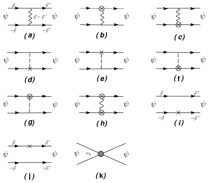
Figure 1: The whole bound state diagrams contributing to positronium energy corrections at the order of $\alpha^{4}$. $\psi$ is schrodinger wavefunction and $c_{4}$ is the leading order result coming from tree-level matching $(c_{4}=c^{(0)}_{4}=-\frac{\pi\alpha}{m^{2}})$.

$$\Delta E_{i}+\Delta E_{j} = 2\int\frac{d^{3}pd^{3}p^{\prime}}{(2\pi)^{6}}\psi^{*}({\bf p^{\prime}})\bigg{[}\frac{-p^{4}(2\pi)^{3}\delta({\bf p}-{\bf p^{\prime}})}{8m^{3}}\bigg{]}\psi(\bf{p})$$ (20)

$$= \frac{-m\alpha^{4}}{16n^{3}(\ell+1/2)}+\frac{3m\alpha^{4}}{64n^{4}}.$$

To obtain positronium energy correction at the order of $\alpha^{4}$ using SS equation, we should omit Figs.(1(i,j)) and calculate the remaining diagrams in Fig.(1) using SS wavefunction. That is obviously leads to the previous result at the order of $\alpha^{4}$ and also extra pieces which start at higher order. These terms are irrelevant to the order of our interest. Meanwhile the result of Eq.(20) can be easily obtained by expanding the Eq.(13) in terms of $\alpha$,

$$E_{n,\ell}=2m\bigg{[}1+\frac{\alpha^{2}}{4(n+\kappa)^{2}}\bigg{]}^{-1/2}=2m-\frac{m\alpha^{2}}{4n^{2}}-\frac{m\alpha^{4}}{16n^{3}(\ell+1/2)}+\frac{3m\alpha^{4}}{64n^{4}}+\dots.$$ (21)

4 $\alpha^{6}$ Positronium Energy Correction

The full calculation of the positronium energy correction at the order of $\alpha^{6}$, using NRQED has been done in reference [10]. In this paper, we focus on the positronium Hyperfine Splitting (HFS) at the order of $\alpha^{6}$ coming from one-photon annihilation [14][2]. To be more specific in the way that the SS wavefunction can be useful in the bound state calculation, we first briefly review the NRQED method in the following subsection.

4.1 Matching and bound state energy shift at NNLO

Since the single photon annihilation of electron-positron occurs in $S=1$ state, one should calculate the diagrams which contain spin-1 Four-Fermion Vertex, $c_{4}(1-\gamma\,\,ann)$. We can write $c_{4}(1-\gamma\,\,ann)=c^{(0)}_{4}(1-\gamma\,\,ann)+c^{(1)}_{4}(1-\gamma\,\,ann)+\dots$ where the superscript ”(0)” and ”(1)” indicate that the coefficients $c_{4}(1-\gamma\,\,ann)$ have been derived using tree-level and one-loop matching, respectively. To obtain the contribution of HFS at the order $\alpha^{6}$, we should perform matching at two-loop level to get $c^{(2)}_{4}(1-\gamma\,\,ann)$. For this purpose, it is more convenient to write:

$$c^{(2)}_{4}(1-\gamma\,\,ann)=c^{(2)}_{4}(1-\gamma\,\,ann)_{PC}+c^{(2)}_{4}(1-\gamma\,\,ann)_{VC},$$ (22)

where PC stands for contribution coming from propagator corrections while VC for vertex corrections. Each terms in right hand-side of Eq.(22) can be obtained from Figs.(2-3).

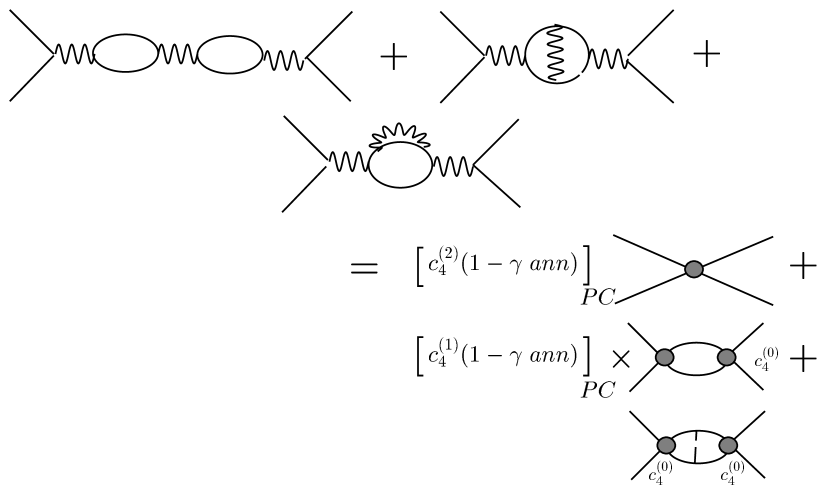
Figure 2: The matching which determines $c^{(2)}_{4}(1-\gamma\,\,ann)_{PC}$ while $c^{(1)}_{4}(1-\gamma\,\,ann)_{PC}$ can be similarly obtained from the one-loop matching procedure.

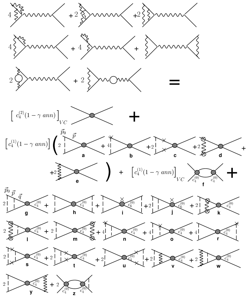
Figure 3: The matching which determines $c^{(2)}_{4}(1-\gamma\,\,ann)_{VC}$ while $c^{(1)}_{4}(1-\gamma\,\,ann)_{VC}$ can be similarly obtained from the one-loop matching procedure.

All the NRQED diagrams which contribute to HFS at the order of $\alpha^{6}$ can be identified using the NRQED power-counting rules[12]. These are shown in Figs.(4-5) which are completely calculated in [8][2]. Diagrams of Figs.(4(k,l,m)) which contain relativistic vertex corrections result in[8]:

$$Fig(\ref{a6a},k)+Fig(\ref{a6a},l)+Fig(\ref{a6a},m)=\frac{m\alpha^{6}}{8}\ln\bigg{(}\frac{\Lambda}{m\alpha}\bigg{)}+\frac{1}{32}m\alpha^{6}+\frac{m\alpha^{5}}{4\pi}\frac{\Lambda}{m}.$$ (23)

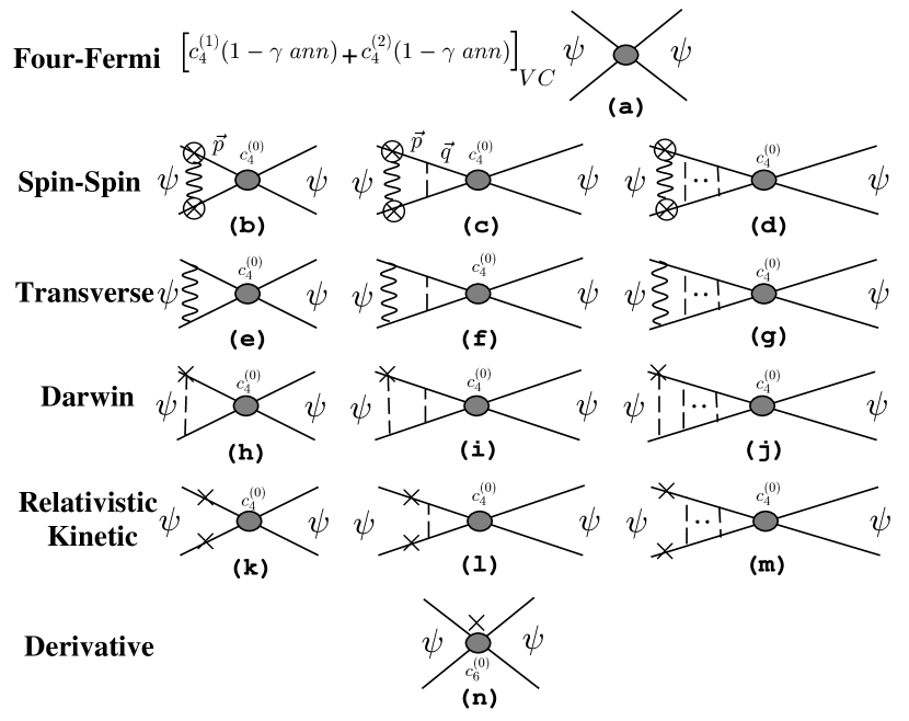
Figure 4: All the bound state diagrams which contribute to $\alpha^{6}$ except the diagrams with the Double Annihilation Interaction. $c_{6}^{(0)}$ is called the Derivative interaction comes from the Taylor expansion of each vertex of the one photon annihilation diagram as well as the photon propagator correction which is equal to $\frac{-2\pi\alpha}{3m^{4}}$.

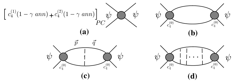
Figure 5: The whole Double Annihilation bound state diagrams.

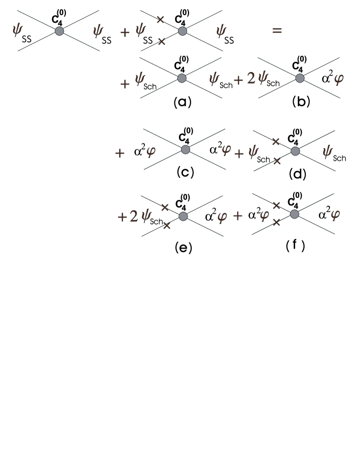
Figure 6: The diagrams at the order $\alpha^{6}$ and higher coming from one photon annihilation at the order $\alpha^{4}$.

4.2 NNLO bound state energy shift using SS wavefunction

As shown in section 2, the whole relativistic kinetic vertex as well as Coulomb vertex can be considered in unperturbed part of the Hamiltonian, Eq.(11). Therefore, one should expect to omit relativistic kinetic vertex and using SS wavefunction instead of Schrodinger wavefunction, in all order of perturbation, to obtain the same results within the framework of NRQED. That is basically reduce the number of counter terms involve in this calculation [15]. Since our goal is to obtain the final result using SS wavefunction, we should omit Figs.(4(k,l,m)) and calculate the remaining diagrams in Fig(4-5) with the SS wavefunction. Straightforward calculations shows that we have the previous result for these diagrams and also extra pieces at higher order than $\alpha^{6}$. At first glance, it seems that there is no way to get the value of Figs.(4k,l,m) which we have omitted, but if we consider the diagrams which contributed to HFS at the order of $\alpha^{4}$ we get some pieces at the higher order. That is basically due to the fact that we should replace $\psi_{Sch}$ with $\psi_{SS}$ in Fig.(1,k) and also using the $p/m$ expansion of relativistic propagator. This means that the Fig.(1,k) should be replaced by the left hand side of Fig.(6). It is easy to show that Fig.(6(a)) leads to the previous result at the order $\alpha^{4}$, while the Figs.(6(c,e,f)) contributes to the higher order than $\alpha^{6}$. The only remaining diagrams relevant to our calculation are the Figs.(6(b,d)):

$$Fig(6(b)) = \frac{4\pi\alpha}{m^{2}}\int\frac{d^{3}p^{\prime}}{(2\pi)^{3}}\psi_{Sch}({\bf p^{\prime}})\int\frac{d^{3}p}{(2\pi)^{3}}\alpha^{2}{\varphi}({\bf p})=\frac{m\alpha^{6}}{8}\ln\bigg{(}\frac{\Lambda}{m\alpha}\bigg{)}+\frac{5}{32}m\alpha^{6},$$ (24)

$$Fig(6(d)) = -\frac{1}{8}m\alpha^{6}+\frac{m\alpha^{5}}{4\pi}\frac{\Lambda}{m}.$$ (25)

The sum of Fig.(6(b)) and Fig.(6(d)) is just equal to (23). It should be noted here that the divergence in the first term of (24) is a direct consequence of the singularity of the SS wavefunction (15). In fact in the Schrodinger case Figs.(2(l,m)) are responsible to cancel the logarithmic divergence coming from the other diagrams while in the SS case this is due to the SS wavefunction.

Summary

In this paper, we have shown that the spinless Salpeter equation (3) correctly predicts the energy spectrum of a non-relativistic two body system such as positronium. In this way we have ignored the relativistic vertex correction in the bound state and therefore the calculations are made easier. On the other hand, although the SS wavefunction is singular at the origin (see Eq.(15)) but this is a crucial need to cancel UV divergence in the bound state system, Eq.(24).

References

• [1] W.E. Caswell and G.P. Lapage, Phys. Lett. 167 B (1986) 437.
• [2] A.H. Hoang, P. Labelle and S.M. Zebarjad, Phys. Rev. A 62 (2000) 012109.
• [3] D.B. Lichtenberg, Int. J. Mod. Phys. A 2 (1987) 1669; I.T. Todorov, Phys. Rev. D 3 (1971) 2351; J.S. Kang and H.J. Schnitzer, Phys. Rev. D 12 (1975) 841; H.W. Crater, hep-ph/9912386, and references therein.
• [4] A.B. Henriques, B.H. Kellett and R.G. Moorhouse, Phys. Lett. 64 B (1976) 85.
• [5] S. Godfrey and N. Isgur, Phys. Rev. D 32 (1985) 189.
• [6] L. Infeld and T.E. Hull, Rev. Mod. Phys., Vol 23, No 1 (1951)21.
• [7] W. Greiner, Relativistic Quantum Mechanics, Springer-Verlag(1990).
• [8] S.M. Zebarjad, McGill Univesity Ph.D. Thesis, (1997).
• [9] C. Itzykson and J.B. Zuber, Quantun Field Theory, McGraw-Hill,(1980).
• [10] A. Czarnecki, K. Melnikov and A. Yelkhovsky, Phys. Rev. A 59 (1999) 4316.
• [11] P.Labelle and S.M. Zebarjad, Can. J. Phys. 77 (1999) 267.
• [12] P. Labelle, Phys. Rev. D 58 (1998) 093013.
• [13] P. Labelle, S.M. Zebarjad and C.P. Burgess, Phys. Rev. D 56 (1997) 8053.
• [14] A. Hoang, P. Labelle and S.M. Zebarjad,Phys. Rev. Lett. 79 (1997) 3387.
• [15] M. Beneke and A.V. Smirnov, Nucl. Phys. B 522 (1998) 321.