Recalculation of Pion Compton Scattering in Perturbative QCD

Abstract

We recalculated pion virtual Compton scattering in perturbative QCD in this paper. Our calculation avoids some deficiencies in existing literatures, and treats real Compton scattering as a limit case in which the mass of the virtual photon equals to zero. Expressions of the hard scattering amplitudes from 10 independent diagrams are given explicitly in the text. By comparing the effects of different distribution amplitudes on the physical observables, we studied the self-consistence of pQCD calculation of this problem.

1 Introduction

Pion virtual Compton scattering (VCS) $\gamma^{*}\pi^{-}\rightarrow\gamma\pi^{-}$ via the reaction $e\pi^{-}\rightarrow e\gamma\pi^{-}$ is observed by SELEX Collaboration at Fermi Lab [1] for the first time. Although in the current available kinematical region, the process can not be predicted precisely in perturbative QCD (pQCD), it is possible to observe such processes in the pQCD-applicable region with the quick development of experimental techniques. Therefore it is meaningful to check the pQCD prediction of this process.

For this problem, Tamazouzt [2] calculated a very similar process, $\gamma\pi^{\pm}\rightarrow\gamma^{*}\pi^{\pm}$; Maina and Torrasso [3] calculated it directly and treated the singular integration appearing in it carefully; Li and Coriano [4] calculated it by a rather different way. One common problem existing in [2] and [4] is: the authors only directly calculated 5 diagrams contributing to the unintegrated amplitude but gave no prescriptions about how to get the other 15 ones, please see fig.2 and captions there. Ref.[3] did not give its expressions for the unintegrated amplitude but claimed consistence with [2]. As was pointed out by the author of [3], the numerical treatments of [2] have some defaults. However, in literature [3], features that deserve further investigations still exist after the revision. For example, a nearly jumping change happened to the phase of $M_{LR}$, please see figure 5 of [3].

Figure 1: Reaction (a) $e\pi^{\pm}\rightarrow e\gamma\pi^{\pm}$ can proceed both through (b)&(c) Bethe-Heitler process and through (d) virtual Compton scattering. In experiments, the two kinds of process can not be separately detected. When the pion momentum change is large enough in the process, the amplitude $M$ of the process (d) $\gamma^{*}\pi^{\pm}\rightarrow\gamma\pi^{\pm}$ can be factorized as (e) $M=\int dxdy\phi(x)H(x,y)\phi(y)$, where $H$ can be computed perturbatively, please see fig.2.

Because of these questions, we decide to recalculate this problem in this paper. It will be shown that, all the deficiencies in the literatures will not exist in our recalculated results.

2 Factorization Theorem of pQCD for Pion VCS

As indicated in the caption of fig.1, a complete physical process $e\pi^{-}\rightarrow e\gamma\pi^{-}$ can take place through two ways, Bethe-Heitler process and virtual Compton scattering. But we will not calculate such a complete process in this paper, please refer to [3] and [5]. We will concentrate on the sub-process $\gamma^{*}\pi^{\pm}\rightarrow\gamma\pi^{\pm}$ and use $M$ denoting the amplitude of it. Besides its inclusion of real Compton scattering as a limit case, it is also meaningful in the preparation for the calculation of the complete process $e\pi^{-}\rightarrow e\gamma\pi^{-}$.

Factorization theorem states that for an exclusive process [6] such as pion VCS $\gamma^{*}\pi^{\pm}\rightarrow\gamma\pi^{\pm}$, the amplitude of it can be written as the following convolution formula,

$$M(p;\epsilon q\rightarrow p^{\prime};\epsilon^{\prime}q^{\prime})=\int dxdy\phi(x,Q)H(xp;\epsilon,q\rightarrow yp^{\prime};\epsilon^{\prime},q^{\prime})\phi(y,Q)\;,$$ (1)

where $p$ denotes the momentum of the incoming pion, $\epsilon$ and $q$ are the polarization vector and momentum of the photon respectively. $x$ denotes one of the momentum fraction of the valence quarks in the incoming pion, and that of the other one will be denoted by $\bar{x}=1-x$. The primed variables or $y$ are associated with outgoing particles.

The pion distribution amplitude $\phi(x,Q)$ in eq.(1) absorbs the long-distance dynamics of $M$ and can be derived by non-perturbative methods [7]. Appearing of $Q$ in it indicates its evolution with the energy scale. In this paper, instead of consideration of such evolution [4, 8], we will study the following five phenomenological models and their effects on the physics predictions [9, 10, 11, 12, 13],

$$\phi_{as}=\sqrt{3}f_{\pi}x(1-x),$$

$$\phi_{bhl}=1.4706\sqrt{3}f_{\pi}x(1-x)\exp[-\frac{0.07043}{x(1-x)}],$$

$$\phi_{cz}=5\sqrt{3}f_{\pi}x(1-x)(2x-1)^{2},$$

$$\phi_{hs}=8.8763\sqrt{3}f_{\pi}x(1-x)(2x-1)^{2}\exp[-\frac{0.07062}{x(1-x)}],$$

$$\phi_{p3}=\sqrt{3}f_{\pi}x(1-x)[0.6016-4.659(2x-1)^{2}+15.52(2x-1)^{4}],$$

(2)

with the pion decay constant $f_{\pi}=93$ MeV and the distribution amplitudes normalized by $\int dx\phi(x)=\sqrt{3}f_{\pi}/6$, please see fig.4 for their explicit shapes. From the figure, we can see that, relative to $\phi_{as}$ and $\phi_{cz}$, the distribution amplitudes $\phi_{bhl}$ and $\phi_{hs}$ suppress the end point region deeply, while function $\phi_{p3}$ intensifies both the near-end-point region and the center region.

Contrary to $\phi(x)$, the hard amplitude $H(xp;\epsilon q\rightarrow yp^{\prime};\epsilon^{\prime}q^{\prime})$ in eq.(1) absorbs short-distance dynamics of the amplitude, and can be calculated perturbatively on the basis of the diagrams in fig.2. With leading Fock state of $\pi^{+}$ ($\pi^{-}$ case is similar),

$$|\pi^{+}(p)\rangle=\frac{1}{\sqrt{2}}\frac{1}{\sqrt{3}}\sum_{i}^{1,2,3}\left[|u^{i}_{\uparrow}(xp)\rangle|\bar{d}^{\bar{i}}_{\downarrow}(\bar{x}p)\rangle-|u^{i}_{\downarrow}(xp)\rangle|\bar{d}^{\bar{i}}_{\uparrow}(\bar{x}p)\rangle\right],$$ (3)

where $i$ and $\bar{i}$ denote the color indices, $H$ can be written as

$$H(xp,\epsilon q\rightarrow yp^{\prime},\epsilon^{\prime}q^{\prime})\sim$$

$$\hskip 22.76228pt\sum_{diag.}\sum_{color}\frac{1}{2}\frac{1}{3}\left[\frac{\bar{u}^{j}_{\uparrow}(yp^{\prime})(...\gamma^{\mu}t^{a}_{ji}...)u^{i}_{\uparrow}(xp)g_{\mu\nu}\delta^{ab}\bar{v}^{\bar{i}}_{\downarrow}(\bar{x}p)(...\gamma^{\nu}t^{b}_{\bar{i}\bar{j}}...)v^{\bar{j}}_{\downarrow}(\bar{y}p^{\prime})}{p_{1}^{2}p_{2}^{2}p_{3}^{2}}\right.$$

$$\hskip 71.13188pt\left.-\frac{\bar{u}^{j}_{\downarrow}(yp^{\prime})(...\gamma^{\mu}t^{a}_{ji}...)u^{i}_{\downarrow}(xp)g_{\mu\nu}\delta^{ab}\bar{v}^{\bar{i}}_{\uparrow}(\bar{x}p)(...\gamma^{\nu}t^{b}_{\bar{i}\bar{j}}...)v^{\bar{j}}_{\uparrow}(\bar{y}p^{\prime})}{p_{1}^{2}p_{2}^{2}p_{3}^{2}}\right],$$

(4)

with the coupling constants $\alpha_{e}$, $\alpha_{s}$ and the charge factor $e_{u}^{2}$ or $e_{u}e_{\bar{d}}$ suppressed for the moment. In eq.(4), $p_{1}$, $p_{2}$ and $p_{3}$ denote the momentum transferred through the two fermion and one gluon propagators; explicit expressions of $(...\gamma^{\mu}t^{a}...)$s depend on the details of diagrams. Using identity of $SU(3)$ color group,

$$t^{a}_{ij}t^{a}_{kl}=\frac{1}{2}(\delta_{il}\delta_{jk}-\frac{1}{3}\delta_{ij}\delta_{kl}),$$ (5)

and some trace making trick, please see [14], eq.(4) can be transformed into the following form

$$H(x,\epsilon q\rightarrow y,\epsilon^{\prime}q^{\prime})=\sum_{diag.}H^{(diag.)}_{\epsilon\epsilon^{\prime}}$$

$$\hskip 91.04872pt=\frac{2}{3}\sqrt{x\bar{x}y\bar{y}}\sum_{diag.}Tr[(\gamma^{\mu}...)_{diag.}\gamma^{5}p\!\!\!/(\gamma_{\mu}...)_{diag.}\gamma^{5}p^{\prime}\!\!\!\!/].$$ (6)

By the usual convention, distribution amplitude $\phi(x)\phi(y)$ will absorb the $\sqrt{x\bar{x}y\bar{y}}$ factor, so it will not be included in our later expressions for $H_{\epsilon\epsilon^{\prime}}$.

Figure 2: Unintegrated (hard) amplitude $H$ can be calculated on the basis of these diagrams. Complete $H$ includes other ten diagrams with the photons attaching to different quark lines, and contributions of those diagrams to the full amplitude $M$ are equal to the above ones except some charge factors.

3 Unintegrated Amplitude of $\gamma^{*}\pi^{\pm}\rightarrow\gamma\pi^{\pm}$

In the center-of-momentum frame of outgoing particles $\gamma$ and $\pi^{\pm}$, please refer to [5], we write all the relevant kinematical variables as follows,

$$p^{\prime\mu}=\frac{\omega+p}{2}(1,-\sin\theta,0,-\cos\theta),$$

$$q^{\prime\mu}=\frac{\omega+p}{2}(1,\sin\theta,0,\cos\theta),$$

$$p^{\mu}=(p,0,0,-p),\ \ q^{\mu}=(\omega,0,0,p),$$ (7)

$$\epsilon_{R}^{\mu}=\frac{1}{\sqrt{2}}(0,-1,-i,0),\ \ \epsilon_{R}^{\prime\mu}=\frac{1}{\sqrt{2}}(0,-\cos\theta,-i,\sin\theta),$$

$$\epsilon_{L}^{\mu}=\frac{1}{\sqrt{2}}(0,1,-i,0),$$

$$\epsilon_{+}^{\mu}=\frac{1}{\sqrt{2}}(1,0,0,1).$$ (8)

Obviously, $\theta$ denotes the scattering angle of the process. According to parity invariance and gauge invariance, we only need to calculate three helicity amplitudes for the purpose of computing the amplitude of the complete physical process $e\pi^{\pm}\rightarrow e\gamma\pi^{\pm}$, please see [3] and [5]. In order to compare with [2], we choose to calculate $H_{RR}$, $H_{LR}$ and $H_{+R}$, while obtain the other five by the following relations,

$$H_{LL}=H_{RR},\ \ H_{RL}=H_{LR},\ \ H_{+L}=H_{+R};$$

$$H_{-R}=-v^{-1}H_{+R},\ \ H_{-L}=-v^{-1}H_{+L}.$$ (9)

After introducing the abbreviation $c=\cos\frac{\theta}{2}$, $s=\sin\frac{\theta}{2}$, $S=(\omega+p)^{2}$, $v=q^{\mu}q_{\mu}/S$ and $\bar{v}=1-v$, we can write all the diagrams contributing to $H$ in more economical forms. The results are shown in table 1-3, where we have transformed the diagrams with two propagators potentially on shell into some equivalent forms in which only one of them can go on shell by the following relation,

$$\frac{f(x,y)}{(x-a(y)+i\epsilon)(x-b(y)+i\epsilon)}=\frac{f(x,y)}{a(y)-b(y)}\left(\frac{1}{x-a(y)+i\epsilon}-\frac{1}{x-b(y)+i\epsilon}\right).$$ (10)

This is very important in the numerical integration. Considering the fact that each diagram of fig.2 has a companion with its photons attached to different quark lines, we include a charge factor for each of the diagrams in the table, where $\frac{5}{9}=e_{u}^{2}+e_{\bar{d}}^{2},\frac{4}{9}=2e_{u}e_{\bar{d}}$.

Table 1 $H^{(diag.)}_{RR}(\frac{1}{S}\alpha_{e}\alpha_{s}$)

$$\begin{array}[]{cccc}\hline\cr\hline\cr{a:}&{\frac{5}{9}\frac{4c^{2}s^{-2}\bar{v}^{-1}}{\bar{x}\bar{y}(x-a-i\epsilon)}}&{f:}&{\frac{5}{9}\frac{4s^{-2}\bar{v}^{-1}}{x\bar{x}\bar{y}}}\\ {b:}&{\frac{5}{9}\frac{4c^{2}s^{-2}\bar{v}^{-1}}{\bar{x}\bar{y}y}}&{g:}&{\frac{5}{9}\frac{4c^{2}s^{-2}\bar{v}^{-1}}{\bar{x}\bar{y}[(1-\bar{v}s^{2})y-v]}}\\ {c:}&{\frac{5}{9}\frac{-4c^{2}s^{-2}\bar{v}^{-1}}{\bar{x}y\bar{y}(x-a+i\epsilon)}}&{h:}&{\frac{5}{9}\frac{-4s^{-2}\bar{v}^{-1}[1-(\bar{v}x+y)s^{2}+2\bar{v}xys^{4}]}{[y(1-\bar{v}s^{2})-v]x\bar{x}\bar{y}}}\\ {d:}&{\frac{4}{9}\frac{4\bar{v}^{-1}[c^{2}+s^{2}(\bar{v}x+v)]}{c^{2}\bar{x}y}(\frac{1}{x-a+i\epsilon}-\frac{1}{x-b+i\epsilon})}&{i:}&{\frac{4}{9}\frac{-4c^{2}}{\bar{y}[y(1-\bar{v}s^{2})-v](x-b+i\epsilon)}}\\ {e:}&{0}&{j:}&{\frac{4}{9}\frac{-4s^{2}\bar{v}^{-1}[y-v+\bar{v}\bar{x}(1-2ys^{2})]}{\bar{x}(1-ys^{2})[y(1-\bar{v}s^{2})-v](x-b+i\epsilon)}}\\ \hline\cr\hline\cr{}\hfil&{a=-\frac{v}{\bar{v}},b=\frac{y-v-y\bar{v}s^{2}}{\bar{v}(1-ys^{2})}}&{}\hfil&{}\hfil\end{array}$$

Table 2 $H^{(diag.)}_{LR}(\frac{1}{S}\alpha_{e}\alpha_{s})$

$$\begin{array}[]{cccc}\hline\cr\hline\cr{a:}&{\frac{5}{9}\frac{4\bar{v}^{-1}}{\bar{x}\bar{y}(x-a+i\epsilon)}}&{f:}&{0}\\ {b:}&{\frac{5}{9}\frac{4\bar{v}^{-1}}{\bar{x}y\bar{y}}}&{g:}&{\frac{5}{9}\frac{4v\bar{v}^{-1}}{\bar{x}\bar{y}[(1-\bar{v}s^{2})y-v]}}\\ {c:}&{0}&{h:}&{\frac{5}{9}\frac{-4\bar{v}^{-1}[y+\bar{v}x(1-2ys^{2})]}{x\bar{x}\bar{y}[(1-\bar{v}s^{2})y-v]}}\\ {d:}&{\frac{4}{9}\frac{4c^{-2}s^{2}}{y}(\frac{1}{x-a+i\epsilon}-\frac{1}{x-b+i\epsilon})}&{i:}&{\frac{4}{9}\frac{-4c^{2}s^{2}y}{\bar{y}(1-ys^{2})[(1-\bar{v}s^{2})y-v](x-b+i\epsilon)}}\\ {e:}&{\frac{4}{9}\frac{-4c^{-2}s^{2}}{y\bar{y}}(\frac{1}{x-a+i\epsilon}-\frac{1}{x-b+i\epsilon})}&{j:}&{\frac{4}{9}\frac{-4s^{2}\bar{v}^{-1}[\bar{y}-\bar{v}\bar{x}(1-2ys^{2})]}{\bar{x}(1-ys^{2})[(1-\bar{v}s^{2})y-v](x-b+i\epsilon)}{}}\\ \hline\cr\hline\cr\end{array}$$

Table 3 $H^{(diag.)}_{+R}(\frac{1}{S}\alpha_{e}\alpha_{s})$

$$\begin{array}[]{cccccccc}\hline\cr\hline\cr{a:}&{\frac{5}{9}\frac{8cs^{-1}}{\bar{x}\bar{y}}}&{f:}&{\frac{5}{9}\frac{4c^{-1}s^{-1}\bar{v}^{-1}(1-2\bar{v}x)}{x\bar{x}\bar{y}}}\\ {b:}&{\frac{5}{9}\frac{4cs^{-1}\bar{v}^{-1}}{\bar{x}y\bar{y}}}&{g:}&{\frac{5}{9}\frac{4cs^{-1}v\bar{v}^{-1}}{\bar{x}\bar{y}[(1-\bar{v}s^{2})y-v]}}\\ {c:}&{\frac{5}{9}\frac{-4cs^{-1}}{\bar{x}y\bar{y}}}&{h:}&{\frac{5}{9}\frac{-4cs^{-1}\bar{v}^{-1}y(1-2\bar{v}s^{2}x)}{x\bar{x}\bar{y}[y(1-\bar{v}s^{2})-v]}}\\ {d:}&{\frac{4}{9}\frac{-4c^{-1}s\bar{v}^{-1}[1-2\bar{v}s^{2}\bar{x}]}{\bar{x}(1-ys^{2})(x-b+i\epsilon)}}&{i:}&{\frac{4}{9}\frac{-4c^{3}sy}{\bar{y}(1-ys^{2})[y(1-\bar{v}s^{2})-v](x-b+i\epsilon)}}\\ {e:}&{\frac{4}{9}\frac{4cs}{\bar{y}(1-ys^{2})(x-b+i\epsilon)}}&{j:}&{\frac{4}{9}\frac{-4cs\bar{v}^{-1}[v-y+2\bar{v}\bar{x}ys^{2}]}{\bar{x}(1-ys^{2})[y(1-\bar{v}s^{2})-v](x-b+i\epsilon)}}\\ \hline\cr\hline\cr\end{array}$$

For $H^{(diag.)}_{RR}$ and $H^{(diag.)}_{LR}$, we compared our expressions with those of [2] in the $v\rightarrow 0$ limit (in [2], it is $R_{b}\rightarrow 0$). Except our consideration of 5 additional independent diagrams labelled $f\to j$, all the other terms, labelled $a\to e$, coincide with [2]. For $H^{(diag.)}_{+R}$, in [2], it is $H_{0R}$, because we employ the convention of [3] for the virtual photon polarization vector, which is different from [2], our expression of it does not coincide with that of [2]. Our convention is very convenient for future calculation of the complete process $e\pi^{\pm}\to e\gamma\pi^{\pm}$.

In the case of $v=0$, by adding all the diagrams in table 2 together, we can get a rather simple expression for $H_{LR}$,

$$H_{LR}=-(\frac{2}{3}+\frac{1}{3})^{2}\frac{8c^{-2}s^{2}}{x(1-y)},$$ (11)

So, in the $v\to 0$ limit, the amplitude $H_{LR}$ is a real number, it has no imaginary part. About this point, literature [15] give a general discussion. It should be notified that [3] has an error or misprint in giving its expression for $H_{LR}|_{v\to 0}$ as $H_{LR}=C_{0}(e_{1}-e_{2})^{2}(x-y)c^{-2}s^{2}$. Obviously, such an unintegrated amplitude will give zero amplitude $M_{LR}$ in the integration after multiplied by a symmetric factor $\phi(x)\phi(y)$, please see eq.(1).

From table 1-3, we can see that, one by one, diagrams in the second row of fig.2 do not equal to those of the first row. From the numerical results of later sections, we will be able to see that, as a total, the second row diagrams also do not equal to those of the first row. So in this problem, the number of independent diagrams is 10 instead of 5. Of course, the total number is 20 as we indicate in the caption of fig.2.

4 Analytical Results of Electron VCS and Qualitative Properties of Pion VCS

From the aspect of experiencing VCS, unpolarized electrons and pions are similar to each other, so we can hope cross sections of VCS on the unpolarized electrons and on pions have similar $v$ and $\theta$ dependence. Because electron has no internal structure, its VCS cross sections can be get analytically. By the same kinematical variables as those of pion VCS, neglecting the mass of the electron, we can get the following expressions for electron VCS $\gamma^{*}_{\epsilon}e\rightarrow\gamma_{\epsilon^{\prime}}e$,

$$d\sigma_{RR}\sim\bar{v}|M_{RR}|^{2}$$

$$\hskip 30.0pt\sim\frac{2}{c^{2}}[(1-v)^{2}+c^{4})]$$ (12)

$$d\sigma_{LR}\sim\bar{v}|M_{LR}|^{2}$$

$$\hskip 30.0pt\sim\frac{1}{c^{2}}[2v^{2}s^{4}]$$ (13)

$$d\sigma_{+R}\sim\bar{v}|M_{+R}|^{2}$$

$$\hskip 30.0pt\sim 2v^{2}s^{2}$$ (14)

Fig.3 illustrated explicit shape of the $v$ and $\theta$ dependence of the cross sections. From the figure, we can easily see that, in both the $R\to R$ and $L\to R$ processes, large angle scattering cross sections dominate over the little angle ones. While, in the $+\to R$ process, the cross sections depend on the scattering angle weakly. As we will indicate in the following, in pion VCS, the same properties of the polarized cross sections persist.

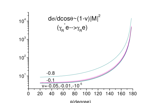
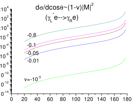
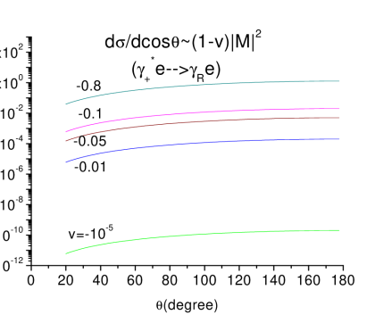
Figure 3: VCS on the unpolarized electron.

5 Numerical Integrations and Results

We perform numerical integrations and give results for the cross sections as well as corresponding phases for different polarized processes in this section.

With eqs.(1), (2), (6) and table 1-3, and using the following relation[16]

$$S^{3}\frac{d\sigma_{\epsilon\epsilon^{\prime}}(\theta)}{d\cos\theta}=\frac{1}{2}\bar{v}S^{4}\frac{d\sigma_{\epsilon\epsilon^{\prime}}(\theta)}{dt}=\bar{v}\frac{S^{2}}{32\pi}|M_{\epsilon\epsilon^{\prime}}|^{2},$$ (15)

and the principle integration formula,

$$\int dxdy\frac{f(x,y)}{x-a(y)+i\epsilon}=\int dxdyP\frac{f(x,y)}{(x-a)}-i\pi\int_{0}^{1}dxdyf(x,y)\delta(x-a)\;,$$

$$\int dxdyP\frac{f(x,y)}{x-a}=\int dxdyP\frac{f(x,y)-f(a,y)}{x-a}+f(a,y)\log\frac{1-a}{a}\;,$$ (16)

we can get reliable numerical results for the cross sections and corresponding phases for different polarization processes. One can see that our treatment of the singular point appearing in the numerical integration is the subtraction method. As was indicated by [16, 17] in the similar calculation for proton Compton scattering, different numerical treatments of the singular points can give consistent results as long as it is applied appropriately.

We get our numerical integrations by VEGAS program [18]. As did by [3], we take $\alpha_{s}=0.3$, $\alpha_{e}=1/137.036$ in numerical computations. Noting the fact that, $H$, thus $M$ varies with $1\over S$, we show the product $S^{3}d\sigma_{\epsilon\epsilon^{\prime}}(\theta)\over d\cos\theta$ instead of $d\sigma_{\epsilon\epsilon^{\prime}(\theta)}\over d\cos\theta$ in final results.

First, in fig.4, using distribution amplitude $\phi_{p3}$, we compared the cross sections of the process $\gamma^{*}_{L}\pi^{\pm}\to\gamma_{R}\pi^{\pm}$ in the following two cases: (i). the unintegrated amplitude includes 10 independent diagrams; (ii). the unintegrated amplitude only includes 5 independent diagrams (the upper part of fig.2). Obviously, the cross sections from the ten diagram contained amplitudes can not be gained by simply multiplying a total factor on those from the five diagram contained ones.

Second, in fig.5, we reconstructed the results of [3] for the cross section $S^{3}\frac{d\sigma_{+R}}{d\cos\theta}$ of pion VCS using distribution amplitudes $\phi_{p3}$. In the right part of this figure, we studied the scattering angle dependence of the cross section when $v\to 0$, by letting $v=-0.8,-0.1,-0.05,-10^{-2},-10^{-5},-10^{-8}$ in stead of $v=-1.0,-0.75,-0.50,-0.25$, as was done in [3].

In fig.6, we illustrated the $v$ and $\theta$ dependence of the cross section and corresponding phases for different polarized processes, with distribution amplitude $\phi_{as}$. For the $+\to R$ process, the cross section decreases with $v\to 0$, and it equals to zero when $v=0$. The scattering angle dependence of it is very similar to that of the electron VCS. As in the electron VCS, both for $L\to R$ and for $R\to R$ processes, large angle scattering cross sections dominate. The difference is, in the little scattering angle regions, the cross section decreases as $v\to 0$, while in the large angle region, the trend reverses. When $v\to 0$, the phase of $M_{LR}\rightarrow 180^{\circ}$, and if we redefine the domain of the phase angle, it can be set to 0.

In fig.7, we compared distribution amplitudes from different models and their effects on the physical observables. We must admit that, relative to those given by $\phi_{as}$ and $\phi_{cz}$, cross sections given by the end-point-region suppressed distribution amplitudes $\phi_{bhl}$ and $\phi_{hs}$ suffer some suppressions. We know that, if the very end point region of the distribution amplitudes has very important contributions to the cross sections of physical processes, pQCD is non-applicable in calculating this problem. Now, our results indicate that this is not the case, so our calculation is self-consistence. Of course, to reduce the differences from distribution amplitudes, careful treatments of the end point region and consideration of the higher order corrections are necessary in further study.

To see this more clearly, we computed another six polarized cross sections for virtual Compton scattering process in fig.8. The upper part of fig.8 corresponds to the $v=-0.05$ case while the down part corresponds to the $v=-0.8$ case. As in fig.7, we can see that the end-point-region suppressed distribution amplitudes still do not give much-suppressed cross sections at most of the scattering angles.

6 Conclusions

We recalculated pion VCS in pQCD in this paper, RCS is treated as a limit case in our framework. Comparisons with existing literatures and with electron VCS are made in the text. Our study of different distribution amplitudes and their effects on the cross sections and corresponding phases of the polarized processes indicates that the behavior of the distribution amplitudes at the very end point region does not have very strong effects on the physical predictions, but careful treatments of the end point region of distribution amplitudes are necessary in the further investigations of this problem.

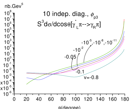
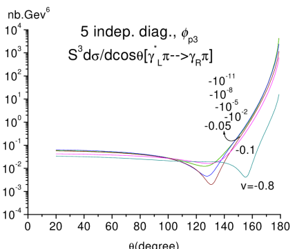
Figure 4: Left part, the cross section $S^{3}\frac{d\sigma_{LR}}{dcos\theta}$ when the hard amplitudes include ten independent diagrams; Right part, the same quantity when the hard amplitudes only include five independent diagrams.

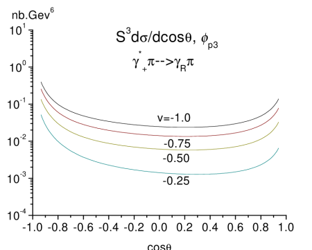
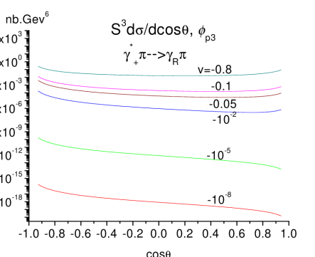
Figure 5: Left part, results reconstructed for $S^{3}\frac{d\sigma_{+R}}{d\cos\theta}$ of [3]. Input photon virtuality approaches to zero in the way $v=-1.0,-0.75,-0.50,-0.25$. Right part, our results for the scattering angle dependence of the cross section when $v$ goes to zero in the way $v=-0.8,-0.1,-10^{-2},-10^{-5},-10^{-8}$.

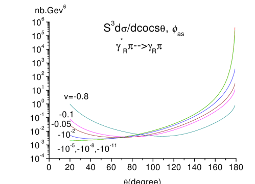
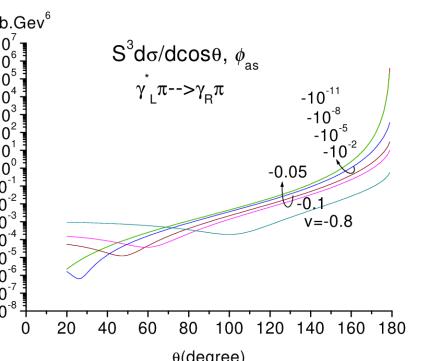
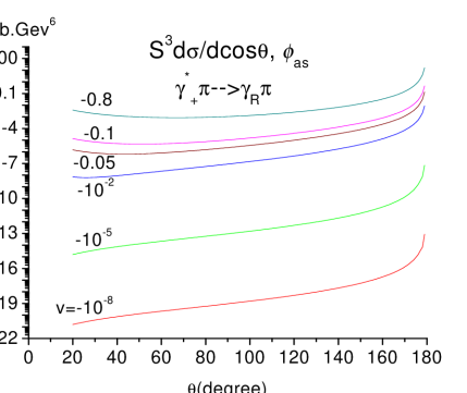
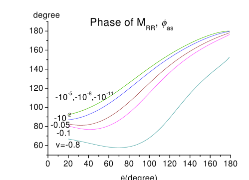
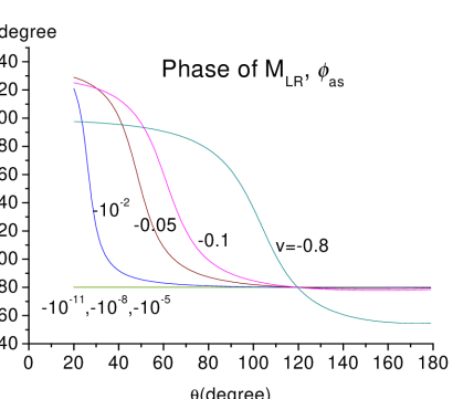
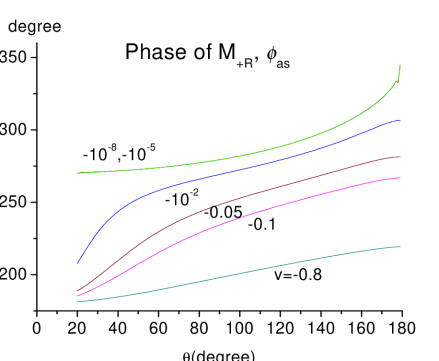
Figure 6: Effects of input photon virtuality on the polarized cross section and corresponding phases. The distribution amplitude involved is $\phi_{as}$. As $v\to 0$, the phase of $M_{LR}\to 180^{\circ}$ asymptotically.

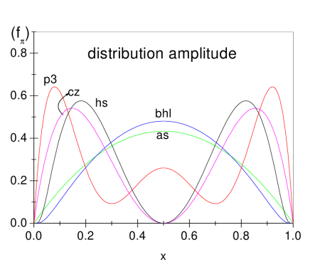
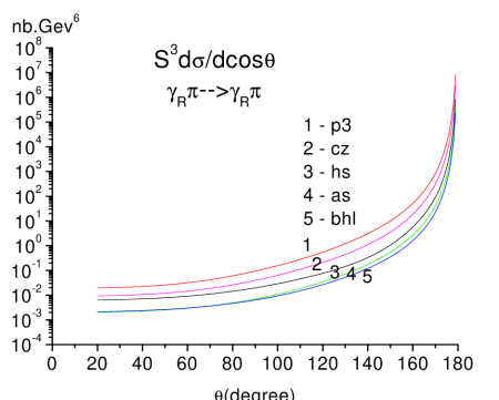
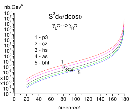
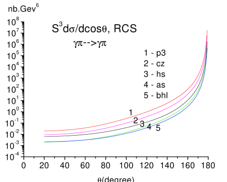
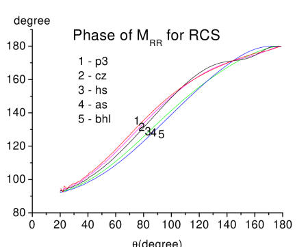
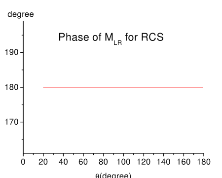
Figure 7: Distribution amplitudes and their effects on the real Compton scattering process. Relative to $\phi_{as}$ and $\phi_{cz}$, functions $\phi_{bhl}$ and $\phi_{hs}$ suppress the end point region deeply, but the corresponding cross sections only suffer little suppressions.

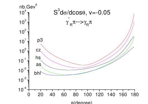
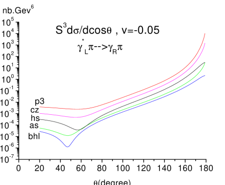
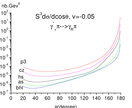
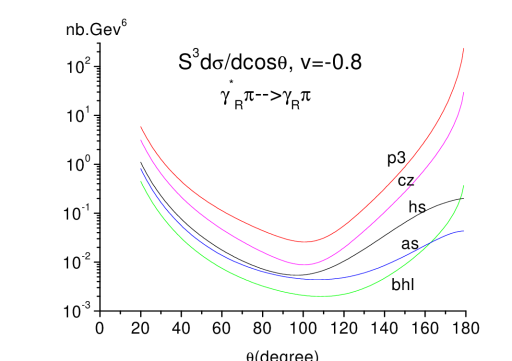
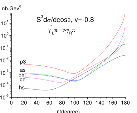
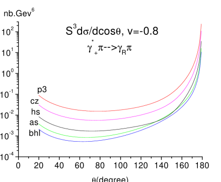
Figure 8: Further study of the effects of distribution amplitudes on the virtual Compton scattering.

References

[1] SELEX Collaboration, hep-ex/0109003.
[2] M. Tamazouzt, Phys. Lett. B 211 (1988) 477.
[3] E. Maina, R. Torasso, Phys. Lett. B 320 (1994)
337.
[4] C. Coriano, H-n. Li, Nucl. Phys. B434 (1995) 535.
[5] G.R. Farrar, H. Zhang, Phys. Rev. D 41
(1990) 3348.
[6] G. P. Lepage, S. J. Brodsky,
Phys. Rev. D 22 (1980) 2157.
[7] M. A. Shifman, A. I. Vainshtein, V. I. Zakharov,
Nucl. Phys. B147 (1979) 385
[8] J. Botts, G. Sterman, Nucl. Phys. B325 (1989) 62;
H-n. Li, G. Sterman, Nucl. Phys. B381 (1992) 129.
[9]V. L. Chernyak, A. R. Zhitnitsky, Phys. Rept. 112 (1984) 173
and
reference there in.
V. L. Chernyak, A. R. Zhitnitsky, Nucl. Phys. B201 (1982) 492.
[10] S. V. Mikhailov, A. V. Radyushkin,
Phys. Rev. D. 45 (1992) 1754;
A. V. Radyushkin, CEBAF-TH-94-13;
V. M. Braun, I. E. Filyalov, Z. Phys. C 44 (1989) 157.
[11] G. R. Farrar, K. Huleihel, H. Zhang,
Nucl. Phys. B349 (1991) 655.
[13] T. Huang, Q.-X. Shen, Z. Phys. C 50 (1991)
139.
[14] R.D. Field, Applications of perturbative QCD, Addison
Wesley Publishing Company, Redwood City, USA, 1989.
[15]
M.T. Grisaru, H.N. Pendleton and P. van Nieuwenhuizen,
Phys. Rev. D 15 (1977) 996;
M.T. Grisaru and
H.N. Pendleton, Nucl. Phys. B124 (1977) 81;
S.J. Parke and T.R.
Taylor,
Phys. Lett. B 157 (1985) 81, err. ibid. B 174 (1986) 465;
M.L. Mangano and S.J. Parke, Phys. Rept. 200 (1991) 301.
[16] T. Brooks, L. Dixon, Phys. Rev. D 62 (2000) 114021.
[17] A. S. Kronfeld, B. Nizic,
Phys. Rev. D44 (1992) 3445, D46 (1992) 2272(E).
[18] G.P. Lepage, J. Comput. Phys. 27 (1978) 192.