Next-to-leading order corrections to
$W+2$ jet and $Z+2$ jet production at hadron colliders

Abstract

We report on QCD radiative corrections to the processes $p{\bar{p}}\to W+\mbox{2~{}jets}$ and $p{\bar{p}}\to Z+\mbox{2~{}jets}$ at the Tevatron. These processes are included in the Monte Carlo program MCFM, which allows the calculation of any infra-red finite variable at next-to-leading order. Due to a better theoretical description of jets at next-to-leading order, some distributions exhibit significant corrections. As expected, the unphysical dependence of theoretical predictions upon the renormalization and factorization scales is greatly reduced compared to leading order. As an example of the predictions that may now be made with MCFM, we present a next-to-leading order estimate of the heavy flavor content of jets produced in association with vector bosons.

I Introduction

In this paper we report on the results of a calculation of the next-to-leading order QCD corrections to the processes,

$$p+\bar{p} \rightarrow W+\mbox{2~{}jets},$$

$$p+\bar{p} \rightarrow Z/\gamma^{*}+\mbox{2~{}jets}.$$ (1)

These reactions will be investigated at the Tevatron, i.e. $p\bar{p}$ collisions at $\sqrt{s}=2$ TeV. Our calculations are equally applicable to the LHC ($pp$ collisions at $\sqrt{s}=14$ TeV). We plan to consider the LHC in a subsequent publication. The results are obtained from the Monte Carlo program MCFM which allows us to obtain full predictions for any infra-red safe variable. In order to obtain fully differential distributions, to which experimental cuts may be applied, various decay modes of the $Z/\gamma^{*}$ intermediate states are included,

$$Z/\gamma^{*} \to e^{-}e^{+}$$

$$Z/\gamma^{*} \to b\bar{b}$$

$$Z \to \sum_{i}\nu_{i}\bar{\nu}_{i}$$ (2)

as well as,

$$W^{+}\to \nu_{e}e^{+}$$ (3)

for the $W^{+}$ decay. In this paper we will only report on leptonic decays of the vector bosons. We use the approximation of massless leptons, so that our results are also valid for the decays $W^{+}\to\nu_{\mu}\mu^{+},W^{+}\to\nu_{\tau}\tau^{+}$ in this approach.

Because of their phenomenological importance, processes involving the production of vector bosons and jets have been considered by many authors. $W$-boson production with two jets was considered at leading order in ref. Kleiss:1985yh ; Ellis:1985vn ; Mangano:1989gs . The same process involving jets at large rapidity was considered in ref. Andersen:2001ja . Vector boson production in association with $n$-jets for $n\leq 4$ is calculated at leading order in refs. Berends:1990ax ; Berends:1989cf . In refs. Ellis:1981hk ; Arnold:1989dp ; Arnold:1989ub ; Giele:dj predictions were made for processes involving a vector boson recoiling against one jet at next-to-leading order. In refs. Giele:1996aa ; Giele:1995kr predictions were made for processes involving $W$ bosons and one heavy quark at next-to-leading order. However to the best of our knowledge this is the first paper to calculate vector boson processes with two jets at next-to-leading order.

In performing these calculations we have used the results of other authors for the crossed reactions $e^{+}e^{-}\to\mbox{4 partons}$ Bern:1997sc and $e^{+}e^{-}\to\mbox{5 partons}$ Nagy:1998bb . Even with the amplitudes in hand, the implementation in a Monte Carlo program requires considerable effort.

In order to highlight the similarities between the effects of radiative corrections on the $W/Z+2~{}{\rm jet}$ rate and the $W/Z+1~{}{\rm jet}$ rate, we will also present some results for the latter process. Such corrections have been known for some time Giele:dj and have provided an invaluable tool for studies at the Tevatron. The inclusion of the $W/Z+1~{}{\rm jet}$ processes in MCFM was useful to understand the issues to be faced in implementing the more complicated $W/Z+2~{}{\rm jet}$ processes.

We will also tie together our results with previous predictions made using MCFM Ellis:1998fv ; Campbell:2000bg to provide a consistent next-to-leading order prediction for the heavy flavor content of jets produced in association with a $W/Z$. Specifically we consider vector boson events containing two tagged $b$-jets. This quantity will be used in assessing the backgrounds to a number of new physics searches at the Tevatron Carena:2000yx . Experimental studies Acosta:2001ct have so far relied upon leading order predictions as theoretical input.

II $\mbox{Hadron}+\mbox{Hadron}\rightarrow W/Z+\mbox{2~{}jets}$

A representative sample of the Born diagrams for the processes,

$$\mbox{parton}+\mbox{parton}\rightarrow W/Z/\gamma^{*}+\mbox{2~{}partons},$$ (4)

is shown in Fig. 1. In the coding of these processes into MCFM we have made an artificial separation between processes involving two quarks, Fig. 1 (a-c) and processes involving four quarks Fig. 1 (d-f).

Figure 1: Sample diagrams for the process $\mbox{parton}+\mbox{parton}\to W/Z+2~{}\mbox{partons}.$ As usual the vector boson is denoted by a wavy line.

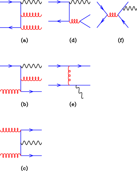
This separation is motivated by the relative size of the contributions at leading order, illustrated in Fig. 2, as well as by the relative complexity of evaluating the different matrix elements.

Figure 2: Color structure of the $W$+2 jet cross section vs. the dijet mass $M_{jj}$ at leading order. Proceeding from the top the five curves are, the total LO result, the two quark process at $O(N)$, the four quark process at $O(1)$, the four quark process at $O(1/N)$ and the two quark process at $O(1/N)$, where $N$ is the number of colors.

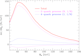
The $2$-quark process at leading $N$ dominates the total, a trend that we find is preserved at next-to-leading order.

We have not recalculated the virtual corrections to the basic Born process which are given by Bern, Dixon and Kosower in ref. Bern:1997sc . These amplitudes have been calculated in the four dimensional helicity scheme, which we consistently use throughout this program.

The real corrections to the basic Born processes, i.e. the processes,

$$\mbox{parton}+\mbox{parton}\rightarrow W/Z/\gamma^{*}+\mbox{3~{}partons}$$ (5)

have been published in Berends:1988yn ; Hagiwara:1988pp ; Nagy:1998bb and a representative sample of the contributing diagrams is shown in Fig. 3.

Figure 3: Sample diagrams for the process $\mbox{parton}+\mbox{parton}\to W/Z+3~{}\mbox{partons}$.

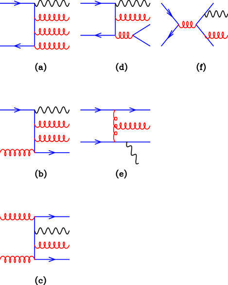
These matrix elements are incorporated in MCFM using the subtraction method of Ellis, Ross and Terrano Ellis:nc ; Ellis:1980wv . In this method, one constructs counterterms having the same singularity structure as the real emission matrix elements, starting from the eikonal formula for soft emission. The basic operating procedure is to create subtraction terms which contain the same singularity structure as the lowest order diagrams, but are simple enough that they are can be integrated over the phase space of the unobserved parton. In order to improve the cancellation, the kinematics of the counterterms are included using the prescription of Catani and Seymour Catani:1996vz . For the case of $W+2$ jets there are 24 different counterterms, each with its own kinematic structure, (a counterevent). The kinematics of the final state partons in the counterevents coincide with the kinematics of the event in the appropriate soft and collinear limits.

II.1 Numerical checks

The matrix elements for hadroproduction of $W/Z$+3 partons contain many singularities which are subtracted by (dipole) counterterms. Although the enumeration of these counterterms is in principle straightforward, the success of the whole program depends on it being implemented correctly. We shall therefore present a few details of the checks which we performed.

The real matrix elements were taken from ref. Nagy:1998bb supplemented in certain cases by our own calculations. The coding of these matrix elements was checked by comparison with routines generated by the program MADGRAPH Stelzer:1994ta powered by HELAS Murayama:1992gi . We cannot use the routines generated by MADGRAPH directly because the resulting code is too slow to implement in a Monte Carlo program which requires many calls to the matrix element routine.

The next step is to verify that the numerical value of the counterterms is in fact equal in magnitude to the real matrix element in the singular limit. This is done by generating sets of points which lie in all of the potentially singular regions and then checking the cancellation of the event and the appropriate counterevent in each limit.

Finally, we must add back the counterterms, suitably integrated over the phase space of the emitted parton. Here it is clearly important to add back exactly what has been subtracted in the previous step. We have tried to structure the code so that the comparison between the two steps is transparent. The integral of the counterterms over the emitted parton sub-space contains singularities, which are regulated using dimensional regularization, in addition to finite contributions. The code is structured so that the finite parts are closely associated with the singular parts. Thus the cancellation of the singular parts, (with the sum of the singular parts of the virtual matrix elements and the Altarelli-Parisi factorization counterterms for the parton distributions), provides some assurance that the finite terms are included correctly.

III Monte Carlo results

III.1 Input parameters

MCFM has a number of default electroweak parameters which we use throughout this paper. They are given in Table 1.

Parameter	Default value	Parameter	Default value
$M_{Z}$	91.187 GeV	$\alpha(M_{Z})$	1/128.89
$\Gamma_{Z}$	2.49 GeV	$G_{F}$	1.16639$\times$10-5
$M_{W}$	80.41 GeV	$g^{2}_{w}$	0.42662 (calculated)
$\Gamma_{W}$	2.06 GeV	$\sin^{2}\theta_{w}$	0.23012 (calculated)

Table 1: Default parameters in the program MCFM.

As noted in the table, some parameters are calculated using the effective field theory approach Georgi:1991ci ,

$$e^{2}=4\pi\alpha(M_{Z}),\;\;g_{w}^{2}=8M^{2}_{W}\frac{G_{F}}{\sqrt{2}},\;\;\sin\theta_{w}=\frac{e^{2}}{g_{w}^{2}}.$$ (6)

For simplicity we have taken the CKM matrix to be diagonal in the $W+2~{}{\rm jets}$ process. As a consequence there are, for example, no $u{\bar{s}}$ initial states for this case. This approximation is not expected to influence any anticipated analyses. For the other processes we retain only the Cabibbo sector of the CKM matrix,

$$V_{CKM}=\left(\begin{array}[]{ccc}0.975&0.222&0\\ 0.222&0.975&0\\ 0&0&1\\ \end{array}\right)\;.$$ (7)

The value of $\alpha_{S}(M_{Z})$ is not adjustable; it is determined by the chosen parton distribution. A collection of modern parton distribution functions is included with MCFM, but here we concentrate only on one of the MRST2001 Martin:2001es sets with $\alpha_{S}(M_{Z})=0.119$. We refer to this set as MRS0119, which is the label used in our program.

III.2 Basic cuts and jet selection

For all the results presented here, we consider only a positively charged $W$ and choose the leptonic decays,

$$W^{+}\to\nu e^{+},\qquad Z/\gamma^{*}\to e^{-}e^{+}.$$ (8)

In this paper we shall present results for the Tevatron collider only and we pick a simple set of cuts accordingly. All leptons satisfy,

$$p_{T}^{\rm lepton}>20~{}{\rm GeV},\qquad|y^{\rm lepton}|<1,$$ (9)

and for the $W$ case there is also a cut on the missing transverse momentum, $p_{T}^{\rm miss}>20~{}{\rm GeV}$. Our final requirement is that the dilepton mass be greater than $15~{}{\rm GeV}$. Although this has no effect in the $W$ case, it prevents the production of soft $e^{-}e^{+}$ pairs which would otherwise be copiously produced by the virtual photon in the $Z/\gamma^{*}$ process.

Jets are found using the Run II $k_{T}$ clustering algorithm Blazey:2000qt with a pseudo-cone of size $R=0.7$, and are also subject to,

$$p_{T}^{\rm jet}>15~{}{\rm GeV},\qquad|y^{\rm jet}|<2.$$ (10)

For the new results on $W,Z+2~{}{\rm jet}$ production, in this paper we will mostly consider events where exactly 2 jets are found by the algorithm, i.e. exclusive 2 jet production. The inclusive production of jets - which would include events with 3 jets at next-to-leading order - is a further option in MCFM that will only be touched on briefly here.

III.3 Scale dependence

The principle motivation for performing a next-to-leading order calculation is to reduce the uncertainties in leading order predictions. In particular, any perturbative prediction contains an unphysical dependence on renormalization and factorization scales (often chosen to be equal, as we shall do here). The magnitude of cross-sections and the shape of differential distributions can vary greatly between two different choices of scale, which is often interpreted as an inherent “theoretical uncertainty” which is then ascribed to the predictions. Another strategy is to argue for a particular choice of scale, based on the physics of the process under consideration.

Figure 4: The scale dependence of the $W$ and $Z$+1 jet predictions, with the factorization and renormalization scales equal and given by $\mu$. The differential distributions $d\sigma/dp_{T}$ are integrated over $15<p_{T}<200~{}{\rm GeV}$, with the basic cuts as described in section III.2.

Figure 5: The scale dependence of the $W$ and $Z$+2 jet differential cross sections, $d\sigma/dM_{jj}$ integrated over $20<M_{jj}<200$ GeV. For more details, see section III.3.

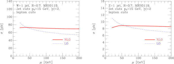
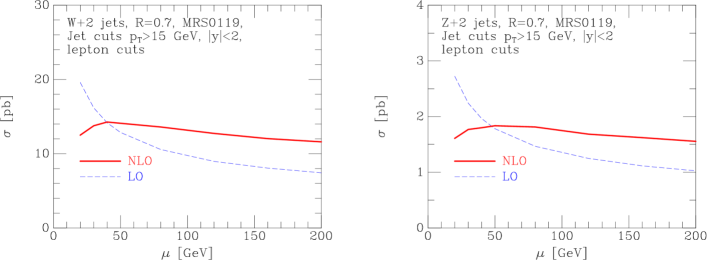
A next-to-leading order calculation is an invaluable tool for investigating the issue of scale dependence. The logarithms that are responsible for the large variations under changes of scale at leading order are exactly canceled through to next-to-leading order. As a result, one expects that next-to-leading order predictions are more stable under such variations. In addition, the next-to-leading order result may provide further evidence to support a particular scale choice that may have been deemed appropriate at leading order.

As an example of expected results, in Figure 4 we show the scale dependence of the exclusive $W$ and $Z$ + 1 jet differential cross-sections $d\sigma/dp_{T}$, integrated over the range $15<p_{T}<200~{}{\rm GeV}$. The next-to-leading order predictions have been known for some time Giele:dj , but here are calculated within our program, MCFM. For both processes, the leading order prediction rises sharply as the scale is decreased, while the corrections produce a far flatter curve that exhibits a much less pronounced dependence on the scale choice.

The corresponding new results for the $2$-jet processes are shown in Figure 5. As in the $1$-jet case, the renormalization and factorization scales are set equal and the basic cuts mentioned in the previous section are applied. In addition, we now use the dijet mass differential distribution, $d\sigma/dM_{jj}$ integrated over $20<M_{jj}<200$ GeV. As anticipated, both processes show a considerable reduction in scale dependence. For example, the ratio of the leading order prediction for the $W$ process using a hard scale $\mu=2m_{W}$ to the result for a far softer scale $\mu=m_{W}/2$ is,

$$\frac{\sigma_{LO}(W+2~{}{\rm jets},\mu=m_{W}/2)}{\sigma_{LO}(W+2~{}{\rm jets},\mu=2m_{W})}=1.7,$$ (11)

while the same ratio at next-to-leading order is only,

$$\frac{\sigma_{NLO}(W+2~{}{\rm jets},\mu=m_{W}/2)}{\sigma_{NLO}(W+2~{}{\rm jets},\mu=2m_{W})}=1.1.$$ (12)

III.4 $p_{T}$ distributions

Once again, we repeat some $W,Z+1$ jet results, in order to highlight both the similarities and the differences with the corresponding $2$-jet distributions.

Figure 6: The jet $p_{T}$ distribution of $W$ and $Z$+1 jet events, evaluated with the hard scale choice, $\mu=80$ GeV.

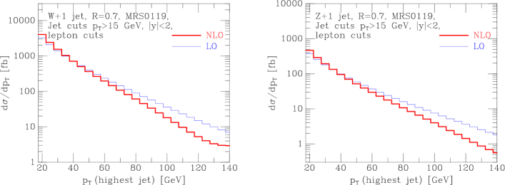
In Figure 6 we show the jet $p_{T}$ distribution for both of the $1$-jet cases, using a relatively hard choice of scale, $\mu=80$ GeV. We first note that since we are considering the exclusive jet cross-section, the rise of the distributions at low $p_{T}$ is limited only by the jet cut, $p_{T}>15$ GeV. At next-to-leading order the distributions change significantly to become much softer. At high $p_{T}$ a single jet is much more likely to radiate a soft parton (that passes the fixed $p_{T}$ cut and is counted as an extra jet), thus removing it from the sample Giele:dj .

Figure 7: The hardest jet $p_{T}$ distribution in $W$ and $Z$+2 jet events, using the scale $\mu=80$ GeV.

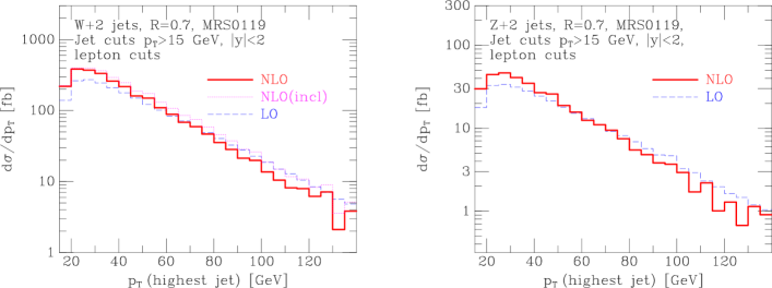
The situation for the $2$-jet processes is shown in Figure 7, where we plot the $p_{T}$ distribution of the hardest jet, again using $\mu=80$ GeV. In contrast with the previous figure, the distributions turn over at small $p_{T}$. If the highest $p_{T}$ jet has a $p_{T}\leq 20$ GeV, there is little phase space for the emission of a second softer jet with $p_{T}>p_{T}^{min}=15$ GeV. We also see that including the radiative corrections softens the distribution considerably, for the same reason as before. For the $W$ case, we also show the inclusive distribution, i.e. the cross section for the production of two or more jets. This ‘fills in’ the high-$E_{T}$ tail of the distribution.

IV Heavy flavor content of jets

IV.1 $\mbox{Hadron}+\mbox{Hadron}\rightarrow W/Z+b+\bar{b}$

We would like to estimate the fraction of $W+2$ jet events that contain two heavy quark jets. We will limit our discussion to $b$ quarks, because they can be tagged with high efficiency. In order to do so, we recall the next-to-leading order results for the production of a $b\bar{b}$ in association with a $W$, reported in Ellis:1998fv . As a reminder to the reader, we work in the approximation in which the $b$ quarks are taken to be massless and we have ignored contributions from processes in which there are two $b$ quarks already present in the initial state. The basic lowest order diagrams for this process are shown in Fig. 8. $Wb\bar{b}$ processes accompanied by up to 4 jets have been considered at tree level in ref. Mangano:2001xp .

Figure 8: Lowest order diagrams for the process $\mbox{parton}+\mbox{parton}\to Wb\bar{b}$.

For the related study including a $Z$ instead of a $W$, we use the results presented in Campbell:2000bg for the production of a $b\bar{b}$ pair in association with a $Z$. The same approximations apply as discussed above for the $W$ case. The notable difference now is that there are more lowest order diagrams, as shown in Fig. 9, including an initial state composed only of gluons. As discussed in Campbell:2000bg , these latter diagrams with initial gluons are believed to be responsible for the sizeable corrections to the basic process at large $m_{b\bar{b}}$.

Figure 9: Sample diagrams for the process $\mbox{parton}+\mbox{parton}\to Zb\bar{b}$.

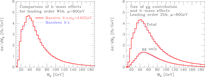
An immediate concern is that neglecting the $b$-quark mass may be unjustified Mangano:1992kp . At low values of $m_{b\bar{b}}$, quark mass effects may be important. To address these concerns, in Figure 10 we compare the lowest order $m_{b\bar{b}}$ distribution calculated using the full mass dependence with the result obtained by setting $m_{b}=0$. There are two effects of introducing a mass for the $b$-quark. Firstly, the phase-space becomes smaller, leading to a reduction of the cross-section. On the other hand, the matrix elements receive extra contributions proportional to powers of $m_{b}^{2}$ which may increase the result. As shown in Figure 10, the matrix element effects dominate around the peak of the distribution where they are as large as 5%. Closer to threshold the phase space effects are dominant. At large $m_{b\bar{b}}$ the quark mass effects are quite small as expected.

Figure 10: Illustration of mass effects in lowest order. $M_{jj}$ is the mass of two tagged $b$-jets.

IV.2 Results

In order to compare the results for $b$-quark jets with those for the whole $2$-jet sample, we will show the differential cross-section as a function of the dijet mass. We use two choices of scale in these analyses, a hard scale $\mu\approx M_{W},M_{Z}=80$ GeV and a softer scale $\mu=40$ GeV. These are the scales used for the plots shown in Figures 11 and 12, where both the leading order and the radiative corrections are shown for comparison.

Figure 11: Comparison of the expected distributions in the dijet mass for untagged $W$+2 jet events and $W$+2 $b$-tagged jet events. A hard scale, $\mu=80~{}{\rm GeV}$, is shown in the left-hand plot and the softer scale, $\mu=40~{}{\rm GeV}$, on the right.

Figure 12: Comparison of the expected distributions in the dijet mass for untagged $Z$+2 jet events and $Z$+2 $b$-tagged jet events. A hard scale, $\mu=80~{}{\rm GeV}$, is shown in the left-hand plot and the softer scale, $\mu=40~{}{\rm GeV}$, on the right.

Figure 13: Ratio of $W/Z$+2 b-tagged jets to $W/Z+2$ jet events in LO and NLO at both $\mu=40$ GeV and $\mu=80$ GeV.

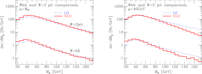
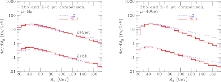
As with the $p_{T}$ distributions of the previous section, the shapes of the distributions change when the QCD corrections are included. For both the $b{\bar{b}}$ and general $2$ jet distributions, the hard scale causes the dijet cross-section to increase at next-to-leading order for small values of $M_{jj}$. The radiative corrections using the soft scale cause a considerable depletion in the cross-section at high $M_{jj}$. However, the shapes of the $b{\bar{b}}$ and $2$ jet distributions appear very similar when compared at the same order of perturbation theory and using the same scale.

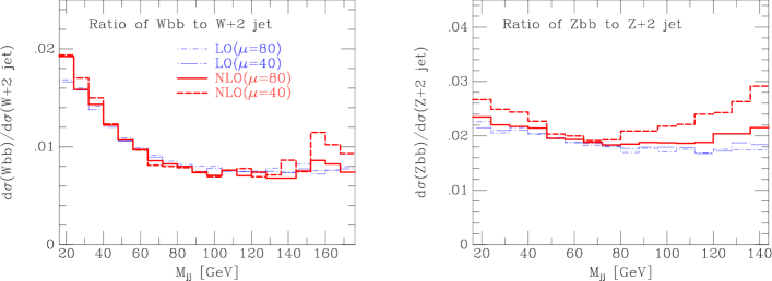
In Fig. 13 we show the cross section for events that contain $2$ $b$-tags divided by the cross section for all two jet events, as a function of the dijet mass. As can be seen, for the $W$ this ratio does not depend very strongly on either the choice of scale or the order in perturbation theory. The percentage falls at low values of $M_{jj}$ until $M_{jj}\sim 60$ GeV, where it becomes approximately constant at $0.8\%$. For the $Z$, the proportion is fairly constant at approximately $2\%$ for all the curves except for the case of next-to-leading order at $\mu=40$ GeV. In this case the percentage rises at high $M_{jj}$. The origin of this effect may be associated with the extra diagrams present in the $Z$ case and requires further study.

V Conclusions

We have presented the first results for the implementation of $W/Z+2~{}$ jet production at next-to-leading order in a general purpose Monte Carlo. An analysis based on exclusive jet production for Run II of the Tevatron shows that the usual benefits of next-to-leading order are realized, among them being a reduced scale dependence and hence an improved normalization for distributions. We also find changes in the shapes of distributions similar to those found in the $1$-jet case. These modifications are reduced if we consider the inclusive cross-section.

We performed an analysis of the heavy flavor content of jets produced in association with a vector boson. For production in association with a $W$, the ratio of $b$-tagged to untagged jets changes very little upon the inclusion of radiative corrections and appears to be predicted very well by perturbation theory.