From the Dyson-Schwinger to the Transport Equation
in the Background Field Gauge of QCD

Abstract

The non-equilibrium quantum field dynamics is usually described in the closed-time-path formalism. The initial state correlations are introduced into the generating functional by non-local source terms. We propose a functional approach to the Dyson-Schwinger equation, which treats the non-local and local source terms in the same way. In this approach, the generating functional is formulated for the connected Green functions and one-particle-irreducible vertices. The great advantages of our approach over the widely used two-particle-irreducible method are that it is much simpler and that it is easy to implement the procedure in a computer program to automatically generate the Feynman diagrams for a given process. The method is then applied to a pure gluon plasma to derive the gauge-covariant transport equation from the Dyson-Schwinger equation in the background covariant gauge. We discuss the structure of the kinetic equation and show its relationship with the classical one. We derive the gauge-covariant collision part and present an approximation in the vicinity of equilibrium. The role of the non-local source kernel in the non-equilibrium system is discussed in the context of a free scalar field.

I Introduction

The ultimate goal of ultra-relativistic nucleus-nucleus collisions is to study the properties of strongly interacting matter under extreme conditions of high energy density rev . Quantum Chromodynamics (QCD) predicts that strongly interacting matter undergoes a phase transition from a state of hadronic constituents to a plasma of unbounded quarks and gluons (QGP) karsch . The QGP is considered as a partonic system being at (or close to) local thermal equilibrium. Thus, to study the conditions for the possible formation of a QGP in heavy-ion collisions one needs to address the question of thermalization of the initially produced partonic medium stock ; baier . There are various theoretical predictions suggesting that the appearance of the QGP could modify the properties of physical quantities that are measured in heavy-ion collisions. The suppression of charmonium production hs was argued to be a possible consequence of the collective effects in the thermalized and deconfined medium. The jet quenching mgxw ; baier1 was predicted to be due to the radiative energy loss of partons penetrating the QGP. Strangeness raf and dilepton vesa production yields could be modified in the thermal QCD medium. A variety of models for the initial conditions in ultra-relativistic heavy-ion collisions suggest that at the early stage the medium is dominated by the gluon degree of freedom sat . The transport equation for a pure gluon plasma is thus of special interest.

The usual treatment of the gluon transport equation is based on the decomposition of the gluon field into a mean field and a quantum fluctuation. Under this approximation the gluon transport equation then describes the kinetics of the quanta in the classical mean field heinz ; geiger ; elze88 . This picture is somewhat similar to what was used while studying the energy loss of the fast parton moving in the soft mean field mgxw ; baier1 . To include the classical chromofield into QCD in a proper way, one uses the background field method of QCD (BG-QCD) introduced by DeWitt and ’t Hooft dewitt ; thooft ; abb81 ; soh86 ; zub75 . The advantage of BG-QCD is that it is formulated in an explicit gauge-invariant manner. The BG-QCD is a very suitable method to describe the properties of a QCD medium created in the initial state of heavy-ion collisions. The time evolution of a quantum system being off equilibrium can be, in principle, obtained by solving the Dyson-Schwinger equation (DSE) defined on a closed-time-path (or the Kadanoff-Baym equations). If the kinetic scale, describing long-range correlations, is much larger than the scale of quantum fluctuations, the DSE may be reduced into a much simpler form of the transport equation by a gradient expansion elze86 ; ctp ; calzetta ; mao . To derive the transport equation in the presence of a classical chromofield in an explicit gauge-invariant or covariant way, one thus combines the BG-QCD method and the closed-time-path (CTP) formalism.

To our knowledge, the first study of the kinetics of a classical particle with non-Abelian gauge degrees of freedom propagating in a non-Abelian classical gauge field is due to Wong wong . There were many efforts in the literature to derive the transport equation for the QCD medium jalilian ; kelly ; litim , particularly by using the BG-QCD method elze90 ; blaizot ; blaizot1 . To our knowledge, the first application of this method was done by Elze elze90 to derive the transport equation for gluons. His approach was based on the Yang-Mills field equation and the second quantization in the operator representation of the quantum field theory. However the equation obtained is in a complicated form. In geiger , the transport equation for the gluon was derived in the conventional QCD by using the light-cone gauge and CTP formalism. The gluon field was decomposed into a hard and a soft part treated as the classical field. This decomposition, however, was not done in a gauge-covariant way. Most recently Blaizot and Iancu have derived the Boltzmann equation for the QCD plasma blaizot , applying the CTP formalism and the BG-QCD method which guarantees the gauge-covariant decomposition of the gauge field.

To derive the Boltzmann equation one needs, in general, to make a set of approximations. This usually involves a gradient expansion of the DSE and the perturbative derivation of the collision term. In Ref. blaizot an additional assumption has been made that the system is close to equilibrium. Consequently, the transport equation for the QCD plasma obtained in Ref. blaizot was linearized with respect to the off-equilibrium fluctuations.

In this paper we propose a different approach to derive the Boltzmann equation for the gluon plasma in the BG-QCD. First we apply the functional approach to the DSE that treats the non-local and local source terms in the same way. We strictly stick to the functional definition of the one-particle-irreducible (1-PI) vertices and the connected Green functions (CGF). Furthermore, we use the DeWitt notation, which, in our opinion, results in a simple structure for the generating functionals. The current approach has a great advantage over the widely used two-particle-irreducible method that it is much simpler and can automatically generate all necessary Feynman diagrams.

In a heuristic discussion on the role of the non-local kernel for a free scalar field, we show that if the initial time is in the remote past the kernel provides only a correction to the homogeneous solution of the DSE and preserves its structure. We also see in this simple model that if the initial time is not in the remote past, the non-local kernel brings the time dependence to the DSE and breaks the assumed structure of the homogeneous solution.

From the DSE, we derive the transport equation in a gauge-covariant way. Our derivation is quite general as it does not require any additional assumptions, such as a special form for the gauge-covariant Green function (GF) or that the system is near equilibrium. Consequently our equation is not linearized with respect to the off-equilibrium fluctuations. We use the background covariant instead of the background Coulomb gauge as was used in Ref. blaizot . Therefore our results preserve an explicit Lorentz covariance and have a compact structure. However, we have to include the ghost fields to cancel the non-physical degrees of freedom of the gauge field. We note that the resulting kinetic equation has a structure similar to the one previously derived in mrow , based on elze88 in QCD and assuming the 2-point gauge-covariant GF (or the Wigner function) to be proportional to the quadratic product of the generators for the fundamental color representation.

We discuss the structure of the kinetic part of the transport equation derived here and compare it with the classical kinetic equation. In the quantum case the kinetic equation describes the time evolution of the gauge-covariant Wigner function, which is a matrix in the adjoint color space. Therefore, it contains many non-Abelian features, which are absent from the well known classical equation. However, a notable result is that, as in the classical case, it contains a term that corresponds to the color precession old . This is the non-Abelian analogue to the Larmor precession for particles with magnetic moments in an external magnetic field. We argue that this term is necessary to preserve the gauge covariance of the resulting transport equation. We also discuss the structure of the kinetic part if the system exhibits only a small deviation from equilibrium.

We derive the gauge-covariant collision part of the Boltzmann equation and present its linearized form with respect to the off-equilibrium fluctuations. Finally applying the transversality condition for the gauge-covariant GF, together with some other approximations, the collision part is further simplified and shows the explicit collision and damping terms.

The paper is organized as follows. In Section II we introduce the basic concept of BG-QCD. In Section III we present two equivalent, in a path-integral sense, methods to derive the classical equation of motion for the gluon. In Section IV, we describe the functional approach to the DSE in the vacuum. We derive the DSE for the 2- and 3-point GF in the background covariant gauge. In Section V we present a derivation of the DSE for the non-equilibrium gluon plasma within the CTP formalism. Section VI contains a heuristic discussion on the role of the non-local source kernel. In Section VII we derive the transport equation from the DSE, applying the gradient expansion. In Section VIII the gauge-covariant collision part is derived and its structure under some approximations is discussed.

In the paper we use $g_{\mu\nu}={\rm diag}(1,-1,-1,-1)$ as the metric tensor. The Lorentz indices are written as subscripts and color indices as superscripts to the relevant quantities. For a pure gluon plasma the color field transforms only under the $SU(3)_{c}$ adjoint representation, thus all color indices are adjoint ones. We use the following notation for the gauge field and its field strength tensor: $A_{\mu}\equiv A_{\mu}^{a}T^{a}$ and $F_{\mu\nu}[A]\equiv F_{\mu\nu}^{a}[A]T^{a}$, where $(T^{a})^{ij}=if^{iaj}$ are the generators of the $SU(3)_{c}$ adjoint representation and $f^{abc}$ are the $SU(3)_{c}$ structure constants. The two-point GF or self-energy (SE) are treated as matrices, thus the color and/or Lorentz indices are sometimes omitted.

For convenience, we list all abbreviations that we use in this paper: background gauge QCD (BG-QCD), Dyson-Schwinger equation (DSE), closed-time-path (CTP), Green function (GF), connected Green function (CGF), one-particle-irreducible (1-PI) and self-energy (SE).

II Background Field Method

Any physical quantity calculated in QCD is gauge invariant and independent of the particular gauge chosen. The classical Lagrangian for the gauge field exhibits an explicit gauge invariance. However, when quantizing the theory in a particular gauge, one introduces the gauge fixing and ghost terms that break the explicit gauge invariance of the Lagrangian. The background field method is such a technique that allows a gauge (background gauge) to be fixed without losing the classical gauge invariance.

In BG-QCD the conventional gluon field is expressed as a sum of a classical background field $A$ and a quantum fluctuation $Q$. The action is given by abb81 ; soh86 ; zub75

$$S=S_{0}+S_{fix}+S_{ghost}+S_{src},$$

$$S_{0}=-\frac{1}{4}\int d^{4}x(F_{\mu\nu}^{i}[A]+D_{\mu}^{ij}[A]Q_{\nu}^{j}-D_{\nu}^{ij}[A]Q_{\mu}^{j}+gf^{ijk}Q_{\mu}^{j}Q_{\nu}^{k})^{2},$$

$$S_{fix}=-\frac{1}{2\alpha}\int d^{4}x(D_{\mu}^{ij}[A]Q^{\mu,j})^{2},$$

$$S_{ghost}=\int d^{4}x\overline{C}^{i}D_{\mu}^{ij}[A]D^{\mu,jk}[A+Q]C^{k},$$

$$S_{src}=\int d^{4}x(J_{\mu}^{i}Q^{\mu,i}+\overline{\xi}^{i}C^{i}+\overline{C}^{i}\xi^{i})\;.$$ (1)

The generating functional for the GF reads

$$Z[A,J,\xi,\overline{\xi}]=\int[dQ][dC][d\overline{C}]\exp(iS),$$ (2)

where the quantum fluctuations $Q_{\mu}^{i}$ of the gluon field are the integration variables in the functional integral; $C^{i},\overline{C}^{i}$ are the ghost and antighost fields; $\overline{\xi}^{i},\xi^{i}$ are the external sources coupling to the ghost and antighost fields respectively. The covariant derivative $D_{\mu}^{ij}[A]$ is defined by $D_{\mu}^{ij}[A]\equiv\partial_{\mu}\delta^{ij}-ig(T^{a})^{ij}A_{\mu}^{a}$. The field strength tensor $F_{\mu\nu}^{i}[A]$ for the background field is given by $F_{\mu\nu}^{i}[A]=\partial_{\mu}A_{\nu}^{i}-\partial_{\nu}A_{\mu}^{i}+gf^{ijk}A_{\mu}^{j}A_{\nu}^{k}$.

There are two types of gauge transformations that leave $Z$ invariant zub75 . The type I transformations are given by

$$A^{\prime}_{\mu} = UA_{\mu}U^{-1}+\frac{i}{g}U\partial_{\mu}U^{-1},$$

$$Q^{\prime}_{\mu} = UQ_{\mu}U^{-1},\,\,\,J^{\prime}_{\mu}=UJ_{\mu}U^{-1},$$

$$C^{\prime}_{\mu} = UCU^{-1},\,\,\,\overline{\xi}^{\prime}=U\overline{\xi}U^{-1},$$

$$\overline{C}^{\prime} = U\overline{C}U^{-1},\,\,\,\xi^{\prime}=U\xi U^{-1}\;,$$ (3)

where $U(x)=\exp(ig\omega^{a}(x)T^{a})$. For an infinitesimal gauge transformation the fields transform as

$$\delta A_{\mu}^{i}=D_{\mu}^{ij}[A]\omega^{j}\;,$$

$$\delta Q_{\mu}^{i}=gf^{ijk}Q_{\mu}^{j}\omega^{k},\,\,\,\,\delta J_{\mu}^{i}=gf^{ijk}J_{\mu}^{j}\omega^{k}\;,$$

$$\delta C^{i}=gf^{ijk}C^{j}\omega^{k},\,\,\,\,\delta\overline{\xi}^{i}=gf^{ijk}\overline{\xi}^{j}\omega^{k}\;,$$

$$\delta\overline{C}^{i}=gf^{ijk}\overline{C}^{j}\omega^{k},\,\,\,\delta\xi^{i}=gf^{ijk}\xi^{j}\omega^{k}\;.$$ (4)

In the type II transformations, the background field does not change, but the gluon field transforms as $Q_{\mu}^{\prime}=U(A_{\mu}+Q_{\mu})U^{-1}+ig^{-1}U\partial_{\mu}U^{-1}$. In this paper, as in Ref. elze90 , type I transformations are relevant where the background field transforms in a conventional way and the gluon transforms like a matter field.

In BG-QCD, we define the generating functional $W[A,J,\xi,\overline{\xi}]$ for the CGF and $\Gamma[A,\langle Q\rangle,\langle C\rangle,\langle\overline{C}\rangle]$ for the 1-PI vertex. Both $W$ and $\Gamma$ are gauge-invariant functionals, thus should be invariant under the gauge transformations (3) and (4). Consequently, one can formulate for $\Gamma$/$W$ a Ward identity that corresponds to this invariance zub75 .

III Equation of motion for gluon and classical field

The equation of motion for the gluon field $Q$ is obtained by using the conventional variation approach. Shifting the gluon field $Q_{\mu}^{i}(x)$ by a small amount $v_{\mu}^{i}(x)$: ${Q^{i}}^{\prime}_{\mu}(x)=Q_{\mu}^{i}(x)+v_{\mu}^{i}(x)$, the variation of the functional $W$ is

$$\delta W=-i\delta\ln Z=Z^{-1}\int[dQ][dC][d\overline{C}]\int d^{4}x\frac{\delta S}{\delta Q_{\mu}^{i}}v_{\mu}^{i}(x)\exp(iS)\;.$$ (5)

Because we only shift a variable of integration in the functional integral, there should be no change for $W$. This requirement leads to the equation of motion for $Q_{\mu}^{i}$:

$$\bigg{\langle}\frac{\delta S}{\delta Q_{\mu}^{i}(x)}\bigg{\rangle}\equiv Z^{-1}\int[dQ][dC][d\overline{C}]\frac{\delta S}{\delta Q_{\mu}^{i}}\exp(iS)=0\;,$$ (6)

where the expectation value $\langle\cdots\rangle$ is taken in the path integral sense. In the absence of the external sources $J$, $\xi$ and $\overline{\xi}$ the equation of motion becomes

$$D_{\nu}^{ij}[A]F^{\nu\mu,j}[A]=\langle j^{\mu,i}\rangle\;,$$ (7)

with the induced current $j$ is given by:

$$j = j_{0}+j_{gf}\;,$$

$$j_{0}^{\mu,i} = -gf^{abc}D_{\nu}^{ia}[A](Q^{\nu,b}Q^{\mu,c})-gf^{ida}Q_{\nu}^{d}(D^{\nu,ab}[A]Q^{\mu,b}-D^{\mu,ab}[A]Q^{\nu,b})$$

$$-g^{2}f^{ida}f^{abc}Q_{\nu}^{d}Q^{\nu,b}Q^{\mu,c}-D_{\nu}^{ij}[A](D^{\nu,jk}[A]Q^{\mu,k}-D^{\mu,jk}[A]Q^{\nu,k})$$

$$-gf^{ijk}Q_{\nu}^{j}F^{\nu\mu,k}[A]\;,$$

$$j_{gf}^{\mu,i} = gf^{kil}\overline{C}^{j}\stackrel{{\scriptstyle\leftarrow}}{{D}}\raisebox{2.15277pt}{${}^{\mu,kj}$}[A]C^{l}-\frac{1}{\alpha}D^{\mu,ij}[A]D^{\nu,jk}[A]Q_{\nu}^{k}\;,$$ (8)

where $j_{0}$ comes from $S_{0}$ and $j_{gf}$ from the ghost and gauge-fixing terms. One can verify that $j$ transforms like a matter field.

In fact, we have $\langle\delta S/\delta Q\rangle=\langle\delta S/\delta A\rangle=0$. The proof can be found in Refs. zub75 and lee73 . From the condition that $\langle\delta S/\delta A\rangle=0$, and after setting all external sources to zero, we obtain

$$D_{\nu}^{ij}[A]F^{\nu\mu,j}[A]=\langle j^{\prime\mu,i}\rangle\;,$$ (9)

where $j^{\prime}$ is defined by

$$j^{\prime} = j_{0}+j^{\prime}_{gf}\;,$$

$$j^{\prime\mu,i}_{gf} = -gf^{kil}\overline{C}^{j}\stackrel{{\scriptstyle\leftarrow}}{{D}}\raisebox{2.15277pt}{${}^{\mu,kj}$}[A]C^{l}-gf^{ijk}\overline{C}^{j}D^{\mu,kl}[A+Q]C^{l}$$ (10)

$$+\frac{1}{\alpha}gf^{ijk}Q^{\mu,k}D_{\nu}^{jl}[A]Q^{\nu,l}\;.$$

Note that $j^{\prime}$ is different from $j$ because $j_{gf}\neq j^{\prime}_{gf}$. However, the expectation values of these two currents are equal. Following from the identity $D_{\mu}^{ij}[A]D_{\nu}^{jk}[A]F^{\nu\mu,k}[A]=0$, we also have $D_{\mu}^{ij}[A]\langle j^{\mu,j}\rangle=D_{\mu}^{ij}[A]\langle j^{\prime\mu,j}\rangle=0$.

IV A Functional Approach to the Dyson-Schwinger Equation in BG-QCD

In the previous section, we have discussed the classical equation of motion for the background and quantum fields. In the following we will show how to obtain the DSE. We will use a convenient functional approach, which has the advantage that the non-local and the local terms are treated in the same way. In our derivation we always use the notation introduced by DeWitt dewitt1 , which gives each formula a simple face and a clear structure. In DeWitt notation the classical action (1) can be written in the following form:

$$S = S_{0}+S_{src}\;,$$

$$S_{0} = \frac{1}{2}\Gamma_{mn}^{(0)}(A^{2})A_{m}A_{n}+\frac{1}{6}\Gamma_{mnp}^{(0)}(A^{3})A_{m}A_{n}A_{p}+\frac{1}{24}\Gamma_{mnpq}^{(0)}(A^{4})A_{m}A_{n}A_{p}A_{q}$$

$$+\frac{1}{2}\Gamma_{mn}^{(0)}(Q^{2})Q_{m}Q_{n}+\frac{1}{6}\Gamma_{mnp}^{(0)}(Q^{3})Q_{m}Q_{n}Q_{p}+\frac{1}{24}\Gamma_{mnpq}^{(0)}(Q^{4})Q_{m}Q_{n}Q_{p}Q_{q}$$

$$+\Gamma_{mn}^{(0)}(AQ)A_{m}Q_{n}+\frac{1}{2}\Gamma_{mnp}^{(0)}(AQ^{2})A_{m}Q_{n}Q_{p}+\frac{1}{2}\Gamma_{mnp}^{(0)}(A^{2}Q)A_{m}A_{n}Q_{p}$$

$$+\frac{1}{6}\Gamma_{mnpq}^{(0)}(A^{3}Q)A_{m}A_{n}A_{p}Q_{q}+\frac{1}{6}\Gamma_{mnpq}^{(0)}(AQ^{3})A_{m}Q_{n}Q_{p}Q_{q}$$

$$+\frac{1}{4}\Gamma_{mnpq}^{(0)}(A^{2}Q^{2})A_{m}A_{n}Q_{p}Q_{q}$$

$$+\Gamma_{mn}^{(0)}(\overline{C}C)\overline{C}_{m}C_{n}+\Gamma_{mnp}^{(0)}(\overline{C}CA)\overline{C}_{m}C_{n}A_{p}+\Gamma_{mnp}^{(0)}(\overline{C}CQ)\overline{C}_{m}C_{n}Q_{p}$$

$$+\Gamma_{mnpq}^{(0)}(\overline{C}CAQ)\overline{C}_{m}C_{n}A_{p}Q_{q}+\frac{1}{2}\Gamma_{mnpq}^{(0)}(\overline{C}CQ^{2})\overline{C}_{m}C_{n}Q_{p}Q_{q}\;,$$

$$S_{src} = J_{m}Q_{m}+\overline{\xi}_{m}C_{m}+\overline{C}_{m}\xi_{m}\;,$$ (11)

where subscripts $m,n,p,q$ represent all necessary indices, including colour, Lorentz and space-time coordinates. The fractions in front of some terms are symmetry factors; $\Gamma_{mnp}^{(0)}(AQ^{2})$, for example, is the bare vertex attaching one $A$ and two $Q$’s. The explicit forms of these bare vertices are given in Appendix A. We use the convention that the repetition of two indices stands for a sum or an integral. Note that the definition of $S_{0}$ has changed from Eq. (1).

From Section III, one knows that the expectation value of the first derivative of $S$ with respect to $Q$ leads to the classical equation of motion. In DeWitt notation this derivative is written as:

$$\frac{\delta S}{\delta Q_{m}} = \Gamma_{mn^{\prime}}^{(0)}(Q^{2})Q_{n^{\prime}}+\Gamma_{n^{\prime}m}^{(0)}(AQ)A_{n^{\prime}}+\Gamma_{m^{\prime}n^{\prime}m}^{(0)}(AQ^{2})A_{m^{\prime}}Q_{n^{\prime}}$$ (12)

$$+\frac{1}{2}\Gamma_{m^{\prime}n^{\prime}m}^{(0)}(A^{2}Q)A_{m^{\prime}}A_{n^{\prime}}+\frac{1}{6}\Gamma_{m^{\prime}n^{\prime}p^{\prime}m}^{(0)}(A^{3}Q)A_{m^{\prime}}A_{n^{\prime}}A_{p^{\prime}}+\frac{1}{2}\Gamma_{m^{\prime}n^{\prime}p^{\prime}m}^{(0)}(A^{2}Q^{2})A_{m^{\prime}}A_{n^{\prime}}Q_{p^{\prime}}$$

$$+\frac{1}{2}\Gamma_{mn^{\prime}p^{\prime}}^{(0)}(Q^{3})Q_{n^{\prime}}Q_{p^{\prime}}+\frac{1}{6}\Gamma_{mn^{\prime}p^{\prime}q^{\prime}}^{(0)}(Q^{4})Q_{n^{\prime}}Q_{p^{\prime}}Q_{q^{\prime}}+\frac{1}{2}\Gamma_{m^{\prime}n^{\prime}p^{\prime}m}^{(0)}(AQ^{3})A_{m^{\prime}}Q_{n^{\prime}}Q_{p^{\prime}}$$

$$+\Gamma_{m^{\prime}n^{\prime}m}^{(0)}(\overline{C}CQ)\overline{C}_{m^{\prime}}C_{n^{\prime}}+\Gamma_{m^{\prime}n^{\prime}p^{\prime}m}^{(0)}(\overline{C}CAQ)\overline{C}_{m^{\prime}}C_{n^{\prime}}A_{p^{\prime}}$$

$$+\Gamma_{m^{\prime}n^{\prime}p^{\prime}m}^{(0)}(\overline{C}CQ^{2})\overline{C}_{m^{\prime}}C_{n^{\prime}}Q_{p^{\prime}}+J_{m}\;.$$

The classical equation of motion then reads

$$\bigg{\langle}\frac{\delta S}{\delta Q_{m}}\bigg{\rangle}=0\,\,\,{\rm or}\,\,\,\bigg{\langle}\frac{\delta S_{0}}{\delta Q_{m}}\bigg{\rangle}=-J_{m}\;.$$ (13)

The explicit form of the equation of motion in the absence of $J_{m}$ is given by Eq. (7). From the 1-PI generating functional, we also have $\delta\Gamma/\delta\langle Q_{m}\rangle=-J_{m}$, consequently we have

$$\bigg{\langle}\frac{\delta S_{0}}{\delta Q_{m}}\bigg{\rangle}=\frac{\delta\Gamma}{\delta\langle Q_{m}\rangle}\;.$$ (14)

From now on we will always refer to $S_{0}$ instead of $S$, we therefore drop the subscript and simply denote it as $S$. Taking the derivative of Eq. (14) with respect to $\langle Q_{p}\rangle$, we have

$$\frac{\delta^{2}\Gamma}{\delta\langle Q_{p}\rangle\delta\langle Q_{m}\rangle} = \frac{\delta J_{n}}{\delta\langle Q_{p}\rangle}\frac{\delta}{\delta J_{n}}\bigg{\langle}\frac{\delta S}{\delta Q_{m}}\bigg{\rangle}=-\frac{\delta^{2}\Gamma}{\delta\langle Q_{p}\rangle\delta\langle Q_{n}\rangle}\frac{\delta}{\delta J_{n}}\bigg{\langle}\frac{\delta S}{\delta Q_{m}}\bigg{\rangle}$$ (15)

$$= -i\Gamma_{pn}(Q^{2})\Big{[}\langle I^{1}_{m}Q_{n}\rangle-\langle Q_{n}\rangle\langle I^{1}_{m}\rangle\Big{]}\;,$$

where $I^{1}_{m}$ is given by Eq. (12), except for the constant terms $A$, $AA$, $AAA$ and $J$, which do not contribute to the DSE. The explicit expression for $\langle I^{1}_{m}Q_{n}\rangle$ reads:

$$\langle I^{1}_{m}Q_{n}\rangle = \Gamma_{mn^{\prime}}^{(0)}(Q^{2})\langle Q_{n^{\prime}}Q_{n}\rangle+\Gamma_{m^{\prime}n^{\prime}m}^{(0)}(AQ^{2})A_{m^{\prime}}\langle Q_{n^{\prime}}Q_{n}\rangle$$ (16)

$$+\frac{1}{2}\Gamma_{m^{\prime}n^{\prime}p^{\prime}m}^{(0)}(A^{2}Q^{2})A_{m^{\prime}}A_{n^{\prime}}\langle Q_{p^{\prime}}Q_{n}\rangle$$

$$+\frac{1}{2}\Gamma_{mn^{\prime}p^{\prime}}^{(0)}(Q^{3})\langle Q_{n^{\prime}}Q_{p^{\prime}}Q_{n}\rangle+\frac{1}{6}\Gamma_{mn^{\prime}p^{\prime}q^{\prime}}^{(0)}(Q^{4})\langle Q_{n^{\prime}}Q_{p^{\prime}}Q_{q^{\prime}}Q_{n}\rangle$$

$$+\frac{1}{2}\Gamma_{m^{\prime}n^{\prime}p^{\prime}m}^{(0)}(AQ^{3})A_{m^{\prime}}\langle Q_{n^{\prime}}Q_{p^{\prime}}Q_{n}\rangle$$

$$+\Gamma_{m^{\prime}n^{\prime}m}^{(0)}(\overline{C}CQ)\langle\overline{C}_{m^{\prime}}C_{n^{\prime}}Q_{n}\rangle+\Gamma_{m^{\prime}n^{\prime}p^{\prime}m}^{(0)}(\overline{C}CAQ)A_{p^{\prime}}\langle\overline{C}_{m^{\prime}}C_{n^{\prime}}Q_{n}\rangle$$

$$+\Gamma_{m^{\prime}n^{\prime}p^{\prime}m}^{(0)}(\overline{C}CQ^{2})\langle\overline{C}_{m^{\prime}}C_{n^{\prime}}Q_{p^{\prime}}Q_{n}\rangle\;.$$

We see that all terms in Eq. (15) are $n$-point correlation functions, or GFs, and can be expressed in terms of CGFs. The relations between the GF and the CGF are given by Eqs. (201) and (202) in Appendix B. A higher-rank CGF can be related to lower-rank CGFs and 1-PI vertices by various identities. These identities are summarized in Eqs. (203) and (204) in Appendix B. For our further discussion we also introduce the following notions and conventions for the GF and CGF. We denote the 2-, 3- and 4-point CGF for $Q$ $G_{mn}(Q^{2})$, $G_{mnp}(Q^{3})$ and $G_{mnpq}(Q^{4})$, respectively. For convenience, sometimes, we also use a short-hand notation $(mn)\equiv G_{mn}(Q^{2})$, $(mnp)\equiv G_{mnp}(Q^{3})$, etc. The 2-, 3- and 4-point CGFs for $Q$ and $\overline{C}$/$C$ are denoted by $G_{mn}(\overline{C}C)$, $G_{mnp}(\overline{C}CQ)$ and $G_{mnpq}(\overline{C}CQ^{2})$, respectively. We also use the following simplified notations: $([mn])\equiv G_{mn}(\overline{C}C)$, $([mn]p)\equiv G_{mnp}(\overline{C}CQ)$, $([mn]pq)\equiv G_{mnpq}(\overline{C}CQ^{2})$ etc.

We treat $A$ and $Q$ as two independent variables. In the last step of the calculations, we always set $\langle Q\rangle$ and all sources to zero. As it is only in the last step that $\langle Q\rangle$ is set to zero, the external sources and background field $A$ are independent of each other in the intermediate steps. This is the difference between our approach and that used in Ref. soh86 . Thus, in deriving the DSE for the 2-point GF, we can drop all terms in Eq. (15) that are proportional to $\langle Q\rangle$ as we need not take further derivative with respect to $\langle Q\rangle$. Note that the correlation function $\langle Q_{m}Q_{n}\rangle$ becomes simply $G_{mn}(Q^{2})$ after dropping the $\langle Q\rangle$ term.

Following the identities

$$\frac{\delta^{2}W}{\delta J_{p}\delta J_{q}}\cdot\frac{\delta^{2}\Gamma}{\delta\langle Q_{p}\rangle\delta\langle Q_{m}\rangle}=-\delta_{qm}\;,$$

$$\frac{\delta^{2}W}{i\delta J_{p}\delta J_{q}}=G_{pq}\;,$$ (17)

we obtain the DSE for 2-point GF from Eq. (15):

$$iG^{-1}_{mp}(Q^{2})=iG^{-1}_{(0)mp}[Q^{2}]+\Pi_{mp}(Q^{2})\;,$$ (18)

where

$$iG^{-1}_{mp}(Q^{2}) = \frac{\delta^{2}\Gamma}{\delta\langle Q_{p}\rangle\delta\langle Q_{m}\rangle}\;,$$

$$iG^{-1}_{(0)mp}[Q^{2}] = \Gamma_{mp}^{(0)}(Q^{2})+\Gamma_{m^{\prime}mp}^{(0)}(AQ^{2})A_{m^{\prime}}+\frac{1}{2}\Gamma_{m^{\prime}n^{\prime}mp}^{(0)}(A^{2}Q^{2})A_{m^{\prime}}A_{n^{\prime}}\;,$$

$$\Pi_{mp}(Q^{2}) = \Pi^{(1)}_{mp}+\Pi^{(2)}_{mp}\;,$$

$$\Pi^{(1)}_{mp}(Q^{2})G_{pq} = \frac{1}{2}\Gamma_{mn^{\prime}p^{\prime}}^{(0)}(Q^{3})\langle Q_{n^{\prime}}Q_{p^{\prime}}Q_{q}\rangle+\frac{1}{6}\Gamma_{mn^{\prime}p^{\prime}q^{\prime}}^{(0)}(Q^{4})\langle Q_{n^{\prime}}Q_{p^{\prime}}Q_{q^{\prime}}Q_{q}\rangle$$

$$+\frac{1}{2}\Gamma_{m^{\prime}n^{\prime}p^{\prime}m}^{(0)}(AQ^{3})A_{m^{\prime}}\langle Q_{n^{\prime}}Q_{p^{\prime}}Q_{q}\rangle\;,$$

$$\Pi^{(2)}_{mp}(Q^{2})G_{pq} = \Gamma_{m^{\prime}n^{\prime}m}^{(0)}(\overline{C}CQ)\langle\overline{C}_{m^{\prime}}C_{n^{\prime}}Q_{q}\rangle+\Gamma_{m^{\prime}n^{\prime}p^{\prime}m}^{(0)}(\overline{C}CAQ)A_{p^{\prime}}\langle\overline{C}_{m^{\prime}}C_{n^{\prime}}Q_{q}\rangle$$ (19)

$$+\Gamma_{m^{\prime}n^{\prime}p^{\prime}m}^{(0)}(\overline{C}CQ^{2})\langle\overline{C}_{m^{\prime}}C_{n^{\prime}}Q_{p^{\prime}}Q_{q}\rangle\;.$$

Note that $i\Pi_{pm}(Q^{2})$ is the normal SE for $Q$; $i\Pi^{(1)}$ is the SE from the gluon loop and $i\Pi^{(2)}$ that from the gluon and ghost loops. Various bare vertices $\Gamma^{(0)}$ can be derived from the classical action (1) by taking the functional derivatives with respect to the field expectation value. The results are summarized in Appendix A.

The DSE (18) can be written in an alternative form:

$$iG^{-1}_{(0)mp}G_{pq}+\Pi_{mp}G_{pq}=i\delta_{mq}\;,$$ (20)

$$G_{nm}iG^{-1}_{(0)mp}+G_{nm}\Pi_{mp}=i\delta_{np}\;.$$ (21)

where we omit the arguments $Q^{2}$ in $G_{mp}(Q^{2})$, $G^{-1}_{mp}(Q^{2})$ and $i\Pi_{pm}(Q^{2})$. We take Eq. (20) as an example to expand and analyse $\Pi_{mp}G_{pq}$. We know that $\Pi_{mp}G_{pq}=\Pi^{(1)}_{mp}G_{pq}+\Pi^{(2)}_{mp}G_{pq}$ where $\Pi^{(1,2)}_{mp}G_{pq}$ are given by Eq. (19). Using Eqs. (201) and (203) from Appendix B, we can expand $\Pi^{(1)}_{mp}G_{pq}$ as follows:

$$\Pi^{(1)}_{mp}G_{pq} = \frac{1}{2}\Gamma_{mn^{\prime}p^{\prime}}^{(0)}(Q^{3})(n^{\prime}p^{\prime}q)+\frac{1}{2}\Gamma_{m^{\prime}n^{\prime}p^{\prime}m}^{(0)}(AQ^{3})A_{m^{\prime}}(n^{\prime}p^{\prime}q)$$ (22)

$$+\frac{1}{6}\Gamma_{mn^{\prime}p^{\prime}q^{\prime}}^{(0)}(Q^{4})\Big{[}i\Gamma_{r^{\prime}s^{\prime}t^{\prime}u^{\prime}}(Q^{4})(r^{\prime}n^{\prime})(s^{\prime}p^{\prime})(t^{\prime}q^{\prime})(u^{\prime}q)$$

$$+3i\Gamma_{r^{\prime}s^{\prime}t^{\prime}}(Q^{3})(r^{\prime}n^{\prime}q)(s^{\prime}p^{\prime})(t^{\prime}q^{\prime})+3(n^{\prime}p^{\prime})(q^{\prime}q)\Big{]}\;.$$

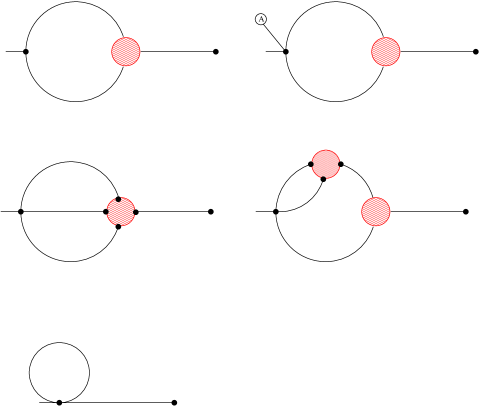
Figure 1: Gluon loop contributions to $\Pi_{mn}G_{np}$, corresponding to Eq. (22).

Note that the fraction in front of each term is a symmetry factor, which is automatically reproduced. In Fig. 1 we show the Feynman diagrams corresponding to the above equation. The solid line there, with two dots at its ends, represents a 2-point full GF. The 3-point full GF is drawn as a shaded circle with three solid-line legs, which have dots at their outer ends. The 1-PI vertex is a shaded circle with all legs amputated; it has dots on the circle that stands for points to which amputated legs are attached. In the same way, we expand $\Pi^{(2)}_{mp}G_{pq}$, which is associated with the ghost loop as

$$\Pi^{(2)}_{mp}G_{pq} = \Gamma_{m^{\prime}n^{\prime}m}^{(0)}(\overline{C}CQ)([m^{\prime}n^{\prime}]q)+\Gamma_{m^{\prime}n^{\prime}p^{\prime}m}^{(0)}(\overline{C}CAQ)A_{p^{\prime}}([m^{\prime}n^{\prime}]q)$$ (23)

$$+\Gamma_{m^{\prime}n^{\prime}p^{\prime}m}^{(0)}(\overline{C}CQ^{2})\Big{\{}([m^{\prime}n^{\prime}]p^{\prime}q)+([m^{\prime}n^{\prime}])(p^{\prime}q)\Big{\}}$$

$$= \Gamma_{m^{\prime}n^{\prime}m}^{(0)}(\overline{C}CQ)([m^{\prime}n^{\prime}]q)+\Gamma_{m^{\prime}n^{\prime}p^{\prime}m}^{(0)}(\overline{C}CAQ)A_{p^{\prime}}([m^{\prime}n^{\prime}]q)$$

$$+\Gamma_{m^{\prime}n^{\prime}p^{\prime}m}^{(0)}(\overline{C}CQ^{2})\Big{\{}i\Gamma_{r^{\prime}s^{\prime}t^{\prime}}(\overline{C}CQ^{2})([m^{\prime}s^{\prime}]q)([r^{\prime}n^{\prime}])(t^{\prime}p^{\prime})$$

$$+i\Gamma_{r^{\prime}s^{\prime}t^{\prime}}(\overline{C}CQ^{2})(m^{\prime}s^{\prime})([r^{\prime}n^{\prime}]q)(t^{\prime}p^{\prime})$$

$$+i\Gamma_{r^{\prime}s^{\prime}t^{\prime}}(\overline{C}CQ^{2})([m^{\prime}s^{\prime}])([r^{\prime}n^{\prime}])(t^{\prime}p^{\prime}q)$$

$$+i\Gamma_{r^{\prime}s^{\prime}t^{\prime}u^{\prime}}(\overline{C}CQ^{2})([m^{\prime}s^{\prime}])([r^{\prime}n^{\prime}])(t^{\prime}p^{\prime})(u^{\prime}q)$$

$$+([m^{\prime}n^{\prime}])(p^{\prime}q)\Big{\}}\;.$$

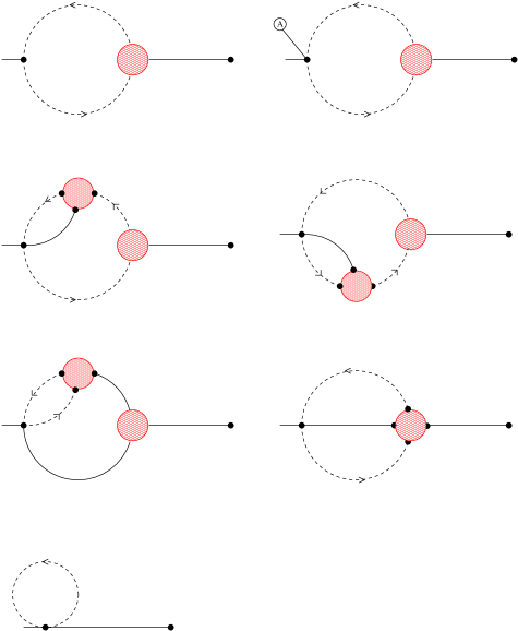
Figure 2: Ghost loop contributions to $\Pi_{mn}G_{np}$, corresponding to Eq. (23).

In the expansion of Eqs. (22) and (23), we have set $\langle Q\rangle$, $\langle C\rangle$ and $\langle\overline{C}\rangle$ to zero. Feynman diagrams corresponding to Eq. (23) are shown in Fig. 2.

Until now we have derived the DSE for the 2-point GF. In the following we extend our analysis to the DSE for the 3-point GF. Taking the derivative with respect to $\langle Q_{l}\rangle$ in Eq. (15), we obtain

$$\frac{\delta}{\delta\langle Q_{l}\rangle}\left[\frac{\delta^{2}\Gamma}{\delta\langle Q_{p}\rangle\delta\langle Q_{m}\rangle}\right]=-i\Gamma_{lpn}(Q^{3})\langle I^{1}_{m}Q_{n}\rangle$$

$$-\Gamma_{pn}(Q^{2})\Gamma_{ll^{\prime}}(Q^{2})\Big{(}\langle I^{1}_{m}Q_{n}Q_{l^{\prime}}\rangle-\langle Q_{l^{\prime}}\rangle\langle I^{1}_{m}Q_{n}\rangle\Big{)}$$

$$+i\Gamma_{lpn}(Q^{3})\langle Q_{n}\rangle\langle I^{1}_{m}\rangle+\Gamma_{pn}(Q^{2})\Gamma_{ll^{\prime}}(Q^{2})$$

$$\cdot\Big{[}\langle I^{1}_{m}\rangle\Big{(}\langle Q_{n}Q_{l^{\prime}}\rangle-\langle Q_{n}\rangle\langle Q_{l^{\prime}}\rangle\Big{)}+\langle Q_{n}\rangle\Big{(}\langle I^{1}_{m}Q_{l^{\prime}}\rangle-\langle I^{1}_{m}\rangle\langle Q_{l^{\prime}}\rangle\Big{)}\Big{]}\;.$$ (24)

After setting $\langle Q\rangle=0$, we have

$$\Gamma_{lpm}(Q^{3}) = -i\Gamma_{lpn}(Q^{3})\langle I^{1}_{m}Q_{n}\rangle-\Gamma_{pn}(Q^{2})\Gamma_{ll^{\prime}}(Q^{2})\langle I^{1}_{m}Q_{n}Q_{l^{\prime}}\rangle$$ (25)

$$+\Gamma_{pn}(Q^{2})\Gamma_{ll^{\prime}}(Q^{2})\langle I^{1^{\prime}}_{m}\rangle\langle Q_{n}Q_{l^{\prime}}\rangle\;,$$

where $I^{1^{\prime}}_{m}$ is as $I^{1}_{m}$ without the $\langle Q\rangle$ terms. From Eq. (15), by dropping the term $\langle Q_{n}\rangle\langle I^{1}_{m}\rangle$, the DSE becomes $\langle I^{1}_{m}Q_{n}\rangle=i\delta_{mn}$. We apply it to the above equation and obtain

$$\langle I^{1}_{m}Q_{n}Q_{p}\rangle=\langle Q_{n}Q_{p}\rangle\langle I^{1^{\prime}}_{m}\rangle\;.$$ (26)

Using Eq. (16), we explicitly write $\langle I^{1}_{m}Q_{n}Q_{p}\rangle$ as follows:

$$\langle I^{1}_{m}Q_{n}Q_{p}\rangle = \Gamma_{mn^{\prime}}^{(0)}(Q^{2})\langle Q_{n^{\prime}}Q_{n}Q_{p}\rangle+\Gamma_{m^{\prime}n^{\prime}m}^{(0)}(AQ^{2})A_{m^{\prime}}\langle Q_{n^{\prime}}Q_{n}Q_{p}\rangle$$ (27)

$$+\frac{1}{2}\Gamma_{m^{\prime}n^{\prime}p^{\prime}m}^{(0)}(A^{2}Q^{2})A_{m^{\prime}}A_{n^{\prime}}\langle Q_{p^{\prime}}Q_{n}Q_{p}\rangle$$

$$+\frac{1}{2}\Gamma_{mn^{\prime}p^{\prime}}^{(0)}(Q^{3})\langle Q_{n^{\prime}}Q_{p^{\prime}}Q_{n}Q_{p}\rangle+\frac{1}{6}\Gamma_{mn^{\prime}p^{\prime}q^{\prime}}^{(0)}(Q^{4})\langle Q_{n^{\prime}}Q_{p^{\prime}}Q_{q^{\prime}}Q_{n}Q_{p}\rangle$$

$$+\frac{1}{2}\Gamma_{m^{\prime}n^{\prime}p^{\prime}m}^{(0)}(AQ^{3})A_{m^{\prime}}\langle Q_{n^{\prime}}Q_{p^{\prime}}Q_{n}Q_{p}\rangle$$

$$+\Gamma_{m^{\prime}n^{\prime}m}^{(0)}(\overline{C}CQ)\langle\overline{C}_{m^{\prime}}C_{n^{\prime}}Q_{n}Q_{p}\rangle$$

$$+\Gamma_{m^{\prime}n^{\prime}p^{\prime}m}^{(0)}(\overline{C}CAQ)A_{p^{\prime}}\langle\overline{C}_{m^{\prime}}C_{n^{\prime}}Q_{n}Q_{p}\rangle$$

$$+\Gamma_{m^{\prime}n^{\prime}p^{\prime}m}^{(0)}(\overline{C}CQ^{2})\langle\overline{C}_{m^{\prime}}C_{n^{\prime}}Q_{p^{\prime}}Q_{n}Q_{p}\rangle\;.$$

We can prove that the disconnected part of $\langle I^{1}_{m}Q_{n}Q_{p}\rangle$ cancels $\langle Q_{n}Q_{p}\rangle\langle I^{1^{\prime}}_{m}\rangle$, hence we write Eq. (26) as

$$iG^{-1}_{(0)mn^{\prime}}[Q^{2}]G_{n^{\prime}np}(Q^{3})=-\Gamma_{mnp}\;,$$ (28)

where the 1-PI vertex $\Gamma_{mnp}$ is defined by

$$\Gamma_{mnp} = \frac{1}{2}\Gamma_{mn^{\prime}p^{\prime}}^{(0)}(Q^{3})\langle Q_{n^{\prime}}Q_{p^{\prime}}Q_{n}Q_{p}\rangle_{c}+\frac{1}{2}\Gamma_{m^{\prime}n^{\prime}p^{\prime}m}^{(0)}(AQ^{3})A_{m^{\prime}}\langle Q_{n^{\prime}}Q_{p^{\prime}}Q_{n}Q_{p}\rangle_{c}$$ (29)

$$+\frac{1}{6}\Gamma_{mn^{\prime}p^{\prime}q^{\prime}}^{(0)}(Q^{4})\langle Q_{n^{\prime}}Q_{p^{\prime}}Q_{q^{\prime}}Q_{n}Q_{p}\rangle_{c}$$

$$+\Gamma_{m^{\prime}n^{\prime}m}^{(0)}(\overline{C}CQ)\langle\overline{C}_{m^{\prime}}C_{n^{\prime}}Q_{n}Q_{p}\rangle_{c}$$

$$+\Gamma_{m^{\prime}n^{\prime}p^{\prime}m}^{(0)}(\overline{C}CAQ)A_{p^{\prime}}\langle\overline{C}_{m^{\prime}}C_{n^{\prime}}Q_{n}Q_{p}\rangle_{c}$$

$$+\Gamma_{m^{\prime}n^{\prime}p^{\prime}m}^{(0)}(\overline{C}CQ^{2})\langle\overline{C}_{m^{\prime}}C_{n^{\prime}}Q_{p^{\prime}}Q_{n}Q_{p}\rangle_{c}\;,$$

and the subscript $c$ stands for the connected part.

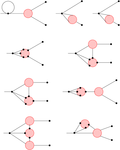
Figure 4: Connected part of 5-point GF $\langle Q_{1}Q_{2}Q_{3}Q_{4}Q_{5}\rangle$, corresponding to Eq. (207).

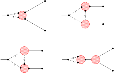
Figure 5: Connected part of 4-point GF $\langle\overline{C}CQ_{1}Q_{2}\rangle$, corresponding to Eq. (209).

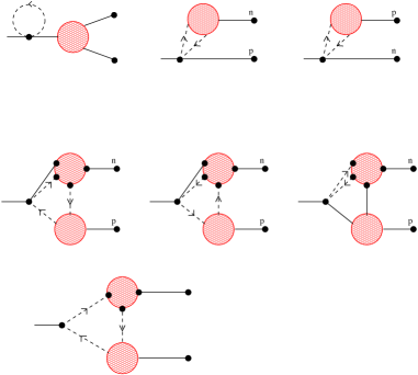
Figure 6: Connected part of 5-point GF $\langle\overline{C}CQ_{1}Q_{2}Q_{3}\rangle$, corresponding to Eq. (210).

We can expand $\Gamma_{mnp}$ term by term. The first term $\frac{1}{2}\Gamma_{mn^{\prime}p^{\prime}}^{(0)}(Q^{3})\langle Q_{n^{\prime}}Q_{p^{\prime}}Q_{n}Q_{p}\rangle_{c}$ in Eq. (29) can be obtained by expressing $\langle Q_{n^{\prime}}Q_{p^{\prime}}Q_{n}Q_{p}\rangle$ by the CGFs of the lower rank. This relation is given by Eq. (205) in Appendix B. We can identify in this relation disconnected GFs $(n^{\prime}p^{\prime})(np)$. After dropping it, we get the connected part $\langle Q_{n^{\prime}}Q_{p^{\prime}}Q_{n}Q_{p}\rangle_{c}$. The corresponding Feynman diagrams are shown in Fig. 3. The second term in Eq. (29) is the same as the first one, except that there is an additional $A$ field attached to the bare vertex. The third, fourth and fifth terms can be expressed in terms of the lower rank CGFs. The resulting relations are given respectively by Eqs. (206-210) in Appendix B. Their corresponding Feynman diagrams are shown in Figs. 4-6.

In this section, we have derived the DSE for the 2- and 3-point GFs. We strictly stick to the functional definition of the 1-PI vertex and the CGF and use the DeWitt notation. Finally, the relations between CGFs and 1-PI vertices were recursively applied to express a higher rank CGF in terms of the lower rank ones and 1-PI vertices. The current approach has the advantage that the non-local terms can be treated in the same way as the local ones. The difference between the local vertex and the non-local one is that the former has a sufficient number of $\delta$-functions to ensure that vertex is at the same space-time point. Another advantage of the current approach is that it can produce all needed Feynman diagrams automatically. Hence it is easy to implement our approach in a computer algorithm, which can automatically generate Feynman diagrams for a given process.

V Dyson-Schwinger Equation in Closed-Time-Path Formalism

The non-equilibrium dynamics is usually described in the CTP formalism schwinger ; keldysh . In this section, we will formulate the DSE in this formalism. The generating functional $Z[J,\xi,\overline{\xi}]$ in the CTP formalism reads:

$$Z[A_{\pm},J_{\pm},\xi_{\pm},\overline{\xi}_{\pm}] = \int[dQ_{+}][dQ_{-}][dC_{+}][dC_{-}][d\overline{C}_{+}][d\overline{C}_{-}]$$

$$\cdot\exp\{iS_{+}-iS_{-}+iK(A_{\pm},Q_{\pm})\}$$

$$S_{+} \equiv S(A_{+},Q_{+},C_{+},\overline{C}_{+},J_{+},\xi_{+},\overline{\xi}_{+})$$

$$S_{-} \equiv S(A_{-},Q_{-},C_{-},\overline{C}_{-},J_{-},\xi_{-},\overline{\xi}_{-})\;,$$ (30)

where the classical action $S$ of BG-QCD is given by Eq. (1). We denote the total action as $S_{CTP}=S_{+}-S_{-}$. We have omitted the kernel $K(A_{\pm},Q_{\pm})$. This is because, as we will see in the next section, the kernel $K$ can be put into the boundary condition. We can treat the $+$ and $-$ quantities as if they were independent. Then, we can derive the Feynman rules according to $S_{CTP}$. The main difference between the tree-level vertices obtained from $S_{CTP}$ and from $S$ lies in that there are negative-type vertices (all time arguments are on the $-$ branch) besides the ordinary positive ones. The vertices of the negative and positive types are the same, except that they have opposite sign. At the tree level, there is also no vertex of mixed type with both positive and negative time arguments.

The 2-point GF for $Q$ is defined by $G=\langle T_{\rm P}Q(x_{1})Q(x_{2})\rangle$, where $T_{\rm P}$ indicates a path-ordered product along the CTP. For simplicity we suppress the Lorentz and colour indices of $Q$ and restore them when necessary. There are four types of 2-point GFs characterized by the time-branch ($+$ or $-$). This can be explicitly written as a matrix:

$$G = \left(\begin{array}[]{cc}\langle{\rm T}Q(x_{1})Q(x_{2})\rangle&\langle Q(x_{2})Q(x_{1})\rangle\\ \langle Q(x_{1})Q(x_{2})\rangle&\langle{\rm T}^{*}Q(x_{1})Q(x_{2})\rangle\end{array}\right)$$ (33)

$$= \left(\begin{array}[]{cc}G^{++}&G^{+-}\\ G^{-+}&G^{--}\end{array}\right)=\left(\begin{array}[]{cc}G^{F}&G^{<}\\ G^{>}&G^{\overline{F}}\end{array}\right)\;,$$ (38)

where $T^{*}$ denotes the counter-time-ordered product; $G^{++}$ ($G^{F}$) is the ordinary GF and its time arguments $t_{1}$ and $t_{2}$ are on the positive time branch; $G^{--}$ ($G^{\overline{F}}$) is the counter-time-ordered or anticausal GF, with both time arguments on the negative time branch; $G^{+-}$ ($G^{<}$) and $G^{-+}$ ($G^{>}$) are correlation functions with time arguments on different branches. The SE has a similar form:

$$\Pi=\left(\begin{array}[]{cc}\Pi^{F}&\Pi^{<}\\ \Pi^{>}&\Pi^{\overline{F}}\end{array}\right)\;.$$ (39)

The GF and the SE can be expressed in the so-called physical representation by using the following unitary transformation:

$$U\left(\begin{array}[]{cc}\Pi^{F}&\Pi^{<}\\ \Pi^{>}&\Pi^{\overline{F}}\end{array}\right)U^{-1}=\left(\begin{array}[]{cc}\Pi^{C}&\Pi^{R}\\ \Pi^{A}&0\end{array}\right)\;,$$ (44)

$$U\left(\begin{array}[]{cc}G^{F}&G^{<}\\ G^{>}&G^{\overline{F}}\end{array}\right)U^{-1}=\left(\begin{array}[]{cc}0&G^{A}\\ G^{R}&G^{C}\end{array}\right)\;,$$ (49)

where

$$U=\frac{1}{\sqrt{2}}\left(\begin{array}[]{cc}1&-1\\ 1&1\end{array}\right),\,\,\,\,U^{-1}=\frac{1}{\sqrt{2}}\left(\begin{array}[]{cc}1&1\\ -1&1\end{array}\right)\;.$$ (50)

Writing the transformation (49) explicitly, we obtain the following relations:

$$G^{A}=G^{F}-G^{>}=G^{<}-G^{\overline{F}},\,\,\,\,\Pi^{A}=\Pi^{F}+\Pi^{>}=-\Pi^{<}-\Pi^{\overline{F}}\;,$$

$$G^{R}=G^{F}-G^{<}=G^{>}-G^{\overline{F}},\,\,\,\,\Pi^{R}=\Pi^{F}+\Pi^{<}=-\Pi^{>}-\Pi^{\overline{F}}\;,$$

$$G^{C}=G^{F}+G^{\overline{F}}=G^{<}+G^{>},\,\,\,\,\Pi^{C}=\Pi^{F}+\Pi^{\overline{F}}=-\Pi^{<}-\Pi^{>}\;.$$ (51)

with $A$, $R$ and $C$ denoting the advanced, retarded and homogeneous GF or SF. Note that there is an additional negative sign for $\Pi^{>,<}$ with respect to $G^{>,<}$. The reason is as follows: the SE tensor $\Pi$ is a 1-PI 2-point GF with external legs amputated, and the two time arguments of $\Pi^{>,<}$ are on different CTP branches. We also know that negative and positive type vertices differ in sign. Therefore, $\Pi^{>,<}$ has an additional negative sign relative to $G^{>,<}$. Such a case, however, does not occur for $\Pi^{\overline{F}}$, because both of its time arguments are on the negative branch; they thus contribute with the same negative signs, which cancel.

Keeping these Feynman rules in mind, we can write the DSE (20) and (21) in the ordinary representation as

$$\left(\begin{array}[]{cc}{\mathcal{D}}+\Pi^{+}&0\\ 0&-{\mathcal{D}}-\Pi^{+}\end{array}\right)_{\mu\nu;ab}(x_{1})\left(\begin{array}[]{cc}G^{F}&G^{<}\\ G^{>}&G^{\overline{F}}\end{array}\right)_{\nu\lambda;bc}(x_{1},x_{2})$$ (56)

$$=ig_{\mu\lambda}\delta_{ac}\delta(x_{1}-x_{2})\left(\begin{array}[]{cc}1&0\\ 0&1\end{array}\right)$$ (59)

$$-\int d^{4}x^{\prime}\left(\begin{array}[]{cc}\Pi^{F}&\Pi^{<}\\ \Pi^{>}&\Pi^{\overline{F}}\end{array}\right)_{\mu\nu;ab}(x_{1},x^{\prime})\left(\begin{array}[]{cc}G^{F}&G^{<}\\ G^{>}&G^{\overline{F}}\end{array}\right)_{\nu\lambda;bc}(x^{\prime},x_{2})\;,$$ (64)

$$\left(\begin{array}[]{cc}G^{F}&G^{<}\\ G^{>}&G^{\overline{F}}\end{array}\right)_{\mu\nu;ab}(x_{1},x_{2})\left(\begin{array}[]{cc}{\mathcal{D}}^{\dagger}+\Pi^{+}&0\\ 0&-{\mathcal{D}}^{\dagger}-\Pi^{+}\end{array}\right)_{\nu\lambda;bc}(x_{2})$$ (69)

$$=ig_{\mu\lambda}\delta_{ac}\delta(x_{1}-x_{2})\left(\begin{array}[]{cc}1&0\\ 0&1\end{array}\right)$$ (72)

$$-\int d^{4}x^{\prime}\left(\begin{array}[]{cc}G^{F}&G^{<}\\ G^{>}&G^{\overline{F}}\end{array}\right)_{\mu\nu;ab}(x_{1},x^{\prime})\left(\begin{array}[]{cc}\Pi^{F}&\Pi^{<}\\ \Pi^{>}&\Pi^{\overline{F}}\end{array}\right)_{\nu\lambda;bc}(x^{\prime},x_{2})\;,$$ (77)

or, in the physical representation, as

$$\left(\begin{array}[]{cc}{\mathcal{D}}+\Pi^{+}&0\\ 0&-{\mathcal{D}}-\Pi^{+}\end{array}\right)_{\mu\nu;ab}(x_{1})\left(\begin{array}[]{cc}G^{R}&G^{C}\\ 0&G^{A}\end{array}\right)_{\nu\lambda;bc}(x_{1},x_{2})$$ (82)

$$=ig_{\mu\lambda}\delta_{ac}\delta(x_{1}-x_{2})\left(\begin{array}[]{cc}1&0\\ 0&1\end{array}\right)$$ (85)

$$-\int d^{4}x^{\prime}\left(\begin{array}[]{cc}\Pi^{C}&\Pi^{R}\\ \Pi^{A}&0\end{array}\right)_{\mu\nu;ab}(x_{1},x^{\prime})\left(\begin{array}[]{cc}0&G^{A}\\ G^{R}&G^{C}\end{array}\right)_{\nu\lambda;bc}(x^{\prime},x_{2})\;,$$ (90)

$$\left(\begin{array}[]{cc}G^{A}&0\\ G^{C}&G^{R}\end{array}\right)_{\mu\nu;ab}(x_{1},x_{2})\left(\begin{array}[]{cc}{\mathcal{D}}^{\dagger}+\Pi^{+}&0\\ 0&-{\mathcal{D}}^{\dagger}-\Pi^{+}\end{array}\right)_{\nu\lambda;bc}(x_{2})$$ (95)

$$=ig_{\mu\lambda}\delta_{ac}\delta(x_{1}-x_{2})\left(\begin{array}[]{cc}1&0\\ 0&1\end{array}\right)$$ (98)

$$-\int d^{4}x^{\prime}\left(\begin{array}[]{cc}0&G^{A}\\ G^{R}&G^{C}\end{array}\right)_{\mu\nu;ab}(x_{1},x^{\prime})\left(\begin{array}[]{cc}\Pi^{C}&\Pi^{R}\\ \Pi^{A}&0\end{array}\right)_{\nu\lambda;bc}(x^{\prime},x_{2})\;.$$ (103)

In Eqs. (64-103), $(x_{1})$ and $(x_{1},x_{2})$ stand for space-time arguments for the functions in front of them. The Lorentz and colour indices are written as subscripts. As an alternative way of presenting the above equations, the local term $\pm\Pi^{+}$ can be absorbed into the definition of $\Pi^{F/\overline{F}}$. In the Feynman gauge ($\alpha=1$) the differential operators ${\mathcal{D}}$ and ${\mathcal{D}}^{\dagger}$ are defined as:

$${\mathcal{D}}^{hi}_{\rho\sigma} = g_{\rho\sigma}D_{\mu}^{ha}[A]D_{\mu}^{ai}[A]-D_{\sigma}^{ha}[A]D_{\rho}^{ai}[A]$$ (104)

$$+\frac{1}{\alpha}D_{\rho}^{ha}[A]D_{\sigma}^{ai}[A]+gf^{hai}F^{a}_{\rho\sigma}[A]$$

$$= g_{\rho\sigma}D_{\mu}^{ha}[A]D_{\mu}^{ai}[A]+2gf^{hai}F^{a}_{\rho\sigma}[A]\;,$$

and

$${\mathcal{D}}^{\dagger;hi}_{\rho\sigma} = g_{\rho\sigma}D_{\mu}^{\dagger;ha}[A]D_{\mu}^{\dagger;ai}[A]+2gf^{hai}F^{a}_{\rho\sigma}[A]\;,$$ (105)

where $D_{\mu}^{ha}[A]=\partial_{\mu}\delta^{ha}+gf^{hba}A_{\mu}^{b}$ is the covariant derivative in the adjoint representation and $D_{\mu}^{\dagger;ha}=\stackrel{{\scriptstyle\leftarrow}}{{\partial}}_{\mu}\delta^{ha}-gf^{hba}A_{\mu}^{b}$ is the conjugate covariant derivative, where the differential operator acts to the left. We note that Eqs. (64-103) are independent of the gauge parameter $\alpha$, owing to the gauge conditions: $D^{ij}_{\mu}[A(x_{1})]G_{\mu\nu}^{jk}(x_{1},x_{2})=0$ and $G^{ij}_{\mu\nu}(x_{1},x_{2})D_{\nu}^{\dagger;jk}[A(x_{2})]=0$.

Some comments about Eqs. (64-105) are in order. First, we recall that Eqs. (104-105) come from the second line of Eq. (19). We write it down explicitly:

$$iG^{-1;hi}_{(0);\rho\sigma}(x,y) = \Gamma_{mp}^{(0)}(Q^{2})+\Gamma_{m^{\prime}mp}^{(0)}(AQ^{2})A_{m^{\prime}}+\frac{1}{2}\Gamma_{m^{\prime}n^{\prime}mp}^{(0)}(A^{2}Q^{2})A_{m^{\prime}}A_{n^{\prime}}$$ (106)

$$= \Big{\{}g_{\rho\sigma}D_{\mu}^{ha}[A(x)]D_{\mu}^{ai}[A(x)]+2gf^{hai}F^{a}_{\rho\sigma}[A(x)]\Big{\}}\delta^{4}(x-y)\;,$$

where labels $m$ and $p$ stand for a group of indices: $m=(x,\rho,h)$ and $p=(y,\sigma,i)$. Multiplying Eq. (106) by $G_{\sigma\xi}^{ij}(y,z)$ and integrating over $y$, Eq. (106) gives

$$\int d^{4}yiG^{-1;hi}_{(0);\rho\sigma}(x,y)G_{\sigma\xi}^{ij}(y,z)$$

$$=\Big{\{}g_{\rho\sigma}D_{\mu}^{ha}[A(x)]D_{\mu}^{ai}[A(x)]+2gf^{hai}F^{a}_{\rho\sigma}[A(x)]\Big{\}}\int d^{4}y\delta^{4}(x-y)G_{\sigma\xi}^{ij}(y,z)$$

$$=\Big{\{}g_{\rho\sigma}D_{\mu}^{ha}[A(x)]D_{\mu}^{ai}[A(x)]+2gf^{hai}F^{a}_{\rho\sigma}[A(x)]\Big{\}}G_{\sigma\xi}^{ij}(x,z)$$

$$={\mathcal{D}}^{hi}_{\rho\sigma}(x)G_{\sigma\xi}^{ij}(x,z)\;.$$ (107)

Multiplying Eq. (106) by $G_{\xi\rho}^{jh}(z,x)$ and integrating over $x$, it becomes:

$$\int d^{4}xG_{\xi\rho}^{jh}(z,x)iG^{-1;hi}_{(0);\rho\sigma}(x,y)$$

$$=\int d^{4}xG_{\xi\rho}^{jh}(z,x)\Big{\{}g_{\rho\sigma}D_{\mu}^{ha}[A(x)]D_{\mu}^{ai}[A(x)]+2gf^{hai}F^{a}_{\rho\sigma}[A(x)]\Big{\}}\delta^{4}(x-y)$$

$$=\int d^{4}xG_{\xi\rho}^{jh}(z,x)\Big{\{}g_{\rho\sigma}D_{\mu}^{\dagger;ha}[A(x)]D_{\mu}^{\dagger;ai}[A(x)]+2gf^{hai}F^{a}_{\rho\sigma}[A(x)]\Big{\}}\delta^{4}(x-y)$$

$$=G_{\xi\rho}^{jh}(z,y)\Big{\{}g_{\rho\sigma}D_{\mu}^{\dagger;ha}[A(y)]D_{\mu}^{\dagger;ai}[A(y)]+2gf^{hai}F^{a}_{\rho\sigma}[A(y)]\Big{\}}$$

$$=G_{\xi\rho}^{jh}(z,y){\mathcal{D}}^{\dagger;hi}_{\rho\sigma}(y)\;,$$ (108)

where the differential operator $\partial$ acting on the $\delta$-function in the second line is changed to $-\stackrel{{\scriptstyle\leftarrow}}{{\partial}}$ in the third line. We notice that $G^{-1;hi}_{(0);\rho\sigma}(x,y)$ in Eq. (106) should be understood as $G^{-1;hi}_{(0);\rho\sigma}(x_{+},y_{+})$, where $x_{+}$ and $y_{+}$ are on the positive time branch. In addition, since $G^{-1;hi}_{(0);\rho\sigma}(x,y)$ is associated with vertices $\Gamma_{mp}^{(0)}(Q^{2})$, $\Gamma_{m^{\prime}mp}^{(0)}(AQ^{2})$ and $\Gamma_{m^{\prime}n^{\prime}mp}^{(0)}(A^{2}Q^{2})$, $G^{-1;hi}_{(0);\rho\sigma}(x_{-},y_{-})$ should have an additional negative sign. This is the reason why there is a negative sign before ${\mathcal{D}}$ and ${\mathcal{D}}^{\dagger}$ in Eqs. (64-103).

Of particular relevance to our further discussion are the specific matrix elements originating from Eqs. (90) and (103). The equations corresponding to the upper-right element of (90) and to the lower-left element of (103) are:

$$\Big{[}{\mathcal{D}}(x_{1})+\Pi^{+}(x_{1})\Big{]}G^{C}(x_{1},x_{2})$$

$$=-\int d^{4}x^{\prime}\Big{[}\Pi^{C}(x_{1},x^{\prime})G^{A}(x^{\prime},x_{2})+\Pi^{R}(x_{1},x^{\prime})G^{C}(x^{\prime},x_{2})\Big{]}\;,$$ (109)

$$G^{C}(x_{1},x_{2})\Big{[}{\mathcal{D}}^{\dagger}(x_{2})+\Pi^{+}(x_{2})\Big{]}$$

$$=-\int d^{4}x^{\prime}\Big{[}G^{R}(x_{1},x^{\prime})\Pi^{C}(x^{\prime},x_{2})+G^{C}(x_{1},x^{\prime})\Pi^{A}(x^{\prime},x_{2})\Big{]}\;,$$ (110)

where, for simplicity, we suppress colour and Lorentz indices in $G$ and $\Pi$, and in particular we regard them as matrices in colour space. We note that the local SE tensor $\Pi^{+}$ can be absorbed into $\Pi^{R}$ and $\Pi^{A}$ to make Eqs. (109) and (110) more compact.

VI Discussions of the non-local source

So far we have not discussed the role of the non-local source term $K(A_{\pm},Q_{\pm})$ in the DSE. The reason is that $K(A_{\pm},Q_{\pm})$ is non-zero only at the initial time and hence can be put to the boundary condition. To illustrate the role of $K$, we consider a simple example of a non-interacting massive scalar field. The classical Lagrangian density is ${\mathcal{L}}=\frac{1}{2}\partial_{\mu}\phi\partial_{\mu}\phi-\frac{1}{2}m^{2}\phi^{2}$. In the CTP approach the role of the initial density matrix is taken by the non-local source kernel $K(\phi_{\pm})$. $K(\phi_{\pm})$ can be expanded into a functional Taylor series in $\phi$. The linear term $K_{a}\phi_{a}$ of this series can be absorbed into the source term $J_{a}\phi_{a}$. The lowest order term, which does have an effect on the dynamics, is the square term $K_{ab}\phi_{a}\phi_{b}$. In this heuristic argument, we neglect higher order terms in this expansion. Using this approximation the DSE has a very simple form:

$$\Big{[}\delta^{4}(x-y)(-\partial_{y}^{2}-m^{2})+K(x,y)\Big{]}\eta\Delta(y,z)=\delta^{4}(x-z)\;,$$ (111)

where $\eta={\rm diag}(1,-1)$; $i\Delta(y,z)$ is a 2-point CTP-form GF which is a $2\times 2$ matrix and $K(x,y)$ is a CTP-form matrix. The solution of the above equation can be written as

$$\Delta(x,y) = \Delta^{(0)}(x,y)-\Delta^{(0)}(x,u_{1})\eta K(u_{1},u_{2})\eta\Delta^{(0)}(u_{2},y)$$ (112)

$$+\Delta^{(0)}(x,u_{1})\eta K(u_{1},u_{2})\eta\Delta^{(0)}(u_{2},u_{3})\eta K(u_{3},u_{4})\eta\Delta^{(0)}(u_{4},y)$$

$$-\cdots\;,$$

where $\Delta^{(0)}(x,y)$ is a solution of the inhomogeneous equation

$$(-\partial_{y}^{2}-m^{2})\eta\Delta^{(0)}(x,y)=\delta^{4}(x-y)\;,$$ (113)

which we call a full propagator. The propagator $\Delta^{(0)}(x,y)$ can be written as the sum of the homogeneous solution and an inhomogeneous one: $\Delta^{(0)}=\Delta^{(0)}_{in}+\Delta^{(0)}_{hom}$, where $i\Delta^{(0)}_{in}(x-y)$ is the Feynman propagator and $\Delta^{(0)}_{hom}(x-y)$ is the solution of the homogeneous equation

$$(-\partial_{y}^{2}-m^{2})\eta\Delta_{hom}(x,y)=0\;.$$ (114)

In momentum space, these propagators become

$$\Delta^{(0)}(p,q) = \Delta^{(0)}(p)\delta^{4}(p-q)\;,$$

$$\Delta^{(0)}(p) = \Delta^{(0)}_{in}(p)+\Delta^{(0)}_{hom}(p)\;,$$ (115)

where $\Delta^{(0)}_{in}(p)$ and $\Delta^{(0)}_{hom}(p)$ are given by

$$\Delta^{(0)}_{in}(p) = \left(\begin{array}[]{cc}\frac{1}{p^{2}-m^{2}+i\epsilon}&0\\ 0&\frac{-1}{p^{2}-m^{2}-i\epsilon}\end{array}\right)\;,$$ (118)

$$\Delta^{(0)}_{hom}(p) = -2\pi i\delta(p^{2}-m^{2})\left(\begin{array}[]{cc}g^{(0)}({\mathbf{p}})&\theta(-p^{0})+g^{(0)}({\mathbf{p}})\\ \theta(p^{0})+g^{(0)}({\mathbf{p}})&g^{(0)}({\mathbf{p}})\end{array}\right)$$ (121)

$$= -2\pi i\delta(p^{2}-m^{2})\Big{[}\lambda_{1}+g^{(0)}({\mathbf{p}})\lambda_{2}\Big{]}\;,$$ (122)

with

$$\lambda_{1}=\left(\begin{array}[]{cc}0&\theta(-p^{0})\\ \theta(p^{0})&0\end{array}\right)\;,\;\;\;\;\lambda_{2}=\left(\begin{array}[]{cc}1&1\\ 1&1\end{array}\right)\;.$$ (123)

In our further discussion we assume that the kernel $K(x_{1},x_{2})$ is given in the following form:

$$K^{ij}(x_{1},x_{2})=\frac{1}{(2\pi)^{3}}K^{ij}({\mathbf{x}}_{1}-{\mathbf{x}}_{2})\delta(x_{1}^{0}-t_{0}^{i})\delta(x_{2}^{0}-t_{0}^{j})\;,$$ (124)

where $i,j=\pm$ and $t_{0}^{+}$ and $t_{0}^{-}$ are, respectively, the starting and ending points of the CTP. The kernel $K^{ij}(x_{1},x_{2})$ is translationally invariant in space, and its Fourier transform reads

$$K^{ij}(k_{1},k_{2}) = \int d^{4}x_{1}d^{4}x_{2}e^{ik_{1}x_{1}}e^{-ik_{2}x_{2}}K^{ij}(x_{1},x_{2})$$

$$= K^{ij}({\mathbf{k}}_{1})\delta^{3}({\mathbf{k}}_{1}-{\mathbf{k}}_{2})\;,$$

$$K^{ij}({\mathbf{k}}_{1}) \equiv \int d^{3}yK^{ij}({\mathbf{y}})e^{-i{\mathbf{k}}_{1}\cdot{\mathbf{y}}}\;,$$ (125)

where we use the same symbol $K$ to denote the kernel in the coordinate and in the momentum space.

Let us now consider the full propagators $\Delta^{(0)}(x,u_{1})$ and $\Delta^{(0)}(u_{n},x)$ appearing in Eq. (112) at the leading and at the end of each term. The values of $u_{1}^{0}$ and $u_{n}^{0}$ are $t_{0}^{+}$ or $t_{0}^{-}$. If one assumes that $t_{0}^{+}\rightarrow-\infty^{+}$ and $t_{0}^{-}=-\infty^{-}$ then $\Delta^{(0);++}(x,u_{1})=\Delta^{(0);>}(x,u_{1})$ since $x^{0}>t_{0}^{+}$ ($x^{0}$ is definite). Similarly, we have: $\Delta^{(0);+-}(x,u_{1})=\Delta^{(0);<}(x,u_{1})$, $\Delta^{(0);-+}(x,u_{1})=\Delta^{(0);>}(x,u_{1})$ and $\Delta^{(0);--}(x,u_{1})=\Delta^{(0);<}(x,u_{1})$. The $++$, $+-$, $-+$ and $--$ components of $\Delta^{(0)}(u_{n},x)$ are of type $<$, $<$, $>$ and $>$, respectively. In momentum space we have

$$\Delta^{(0)}_{h}(p) = -2\pi i\delta(p^{2}-m^{2})\Big{[}\lambda_{3}+g^{(0)}({\mathbf{p}})\lambda_{2}\Big{]}\;,$$

$$\Delta^{(0)}_{e}(q) = -2\pi i\delta(q^{2}-m^{2})\Big{[}\lambda_{4}+g^{(0)}({\mathbf{q}})\lambda_{2}\Big{]}\;,$$ (126)

where the subscripts $h$ and $e$ denote the leading and the end propagator, respectively, and $\lambda_{3}$ and $\lambda_{4}$ are defined as

$$\lambda_{3}=\left(\begin{array}[]{cc}\theta(p^{0})&\theta(-p^{0})\\ \theta(p^{0})&\theta(-p^{0})\end{array}\right)\;,\;\;\;\;\lambda_{4}=\left(\begin{array}[]{cc}\theta(-q^{0})&\theta(-q^{0})\\ \theta(q^{0})&\theta(q^{0})\end{array}\right)\;.$$ (127)

The propagators $\Delta^{0}(u_{i},u_{i+1})$ appearing in Eq. (112) have both of their time variables pinched at $t_{0}$. Thus, they are not bound by the above arguments and their four components are equal. Finally, in momentum space, the full propagator (112) becomes

$$\Delta(p,q)=\Delta^{(0)}(p)\delta^{4}(p-q)-\Delta^{(0)}_{h}(p){\mathcal{K}}({\mathbf{p}})\Delta^{(0)}_{e}(q)\delta^{3}({\mathbf{p}}-{\mathbf{q}})\;,$$ (128)

where ${\mathcal{K}}({\mathbf{p}})$ is given by

$${\mathcal{K}}({\mathbf{p}}) = \eta K({\mathbf{p}})\eta-\eta K({\mathbf{p}})\eta\tilde{\Delta}^{(0)}({\mathbf{p}})\lambda_{2}\eta K({\mathbf{p}})\eta$$ (129)

$$+\eta K({\mathbf{p}})\eta\tilde{\Delta}^{(0)}({\mathbf{p}})\lambda_{2}\eta K({\mathbf{p}})\eta\tilde{\Delta}^{(0)}({\mathbf{p}})\lambda_{2}\eta K({\mathbf{p}})\eta-\cdots\;,$$

and $\tilde{\Delta}^{(0)}({\mathbf{p}})=\int dp^{0}\Delta^{(0)}(p)$. Collecting the sum in the above equation, we obtain:

$${\mathcal{K}}^{++}({\mathbf{p}}) = C\Big{[}(1+AB_{2})K^{++}({\mathbf{p}})+AB_{1}K^{+-}({\mathbf{p}})\Big{]}\;,$$

$${\mathcal{K}}^{+-}({\mathbf{p}}) = C\Big{[}-(1+AB_{1})K^{+-}({\mathbf{p}})-AB_{2}K^{++}({\mathbf{p}})\Big{]}\;,$$

$${\mathcal{K}}^{-+}({\mathbf{p}}) = C\Big{[}-(1+AB_{2})K^{-+}({\mathbf{p}})-AB_{1}K^{--}({\mathbf{p}})\Big{]}\;,$$

$${\mathcal{K}}^{--}({\mathbf{p}}) = C\Big{[}(1+AB_{1})K^{--}({\mathbf{p}})+AB_{2}K^{-+}({\mathbf{p}})\Big{]}\;,$$ (130)

where $A=\tilde{\Delta}^{(0)}({\mathbf{p}})$, $B_{1}=K^{++}({\mathbf{p}})-K^{-+}({\mathbf{p}})$, $B_{2}=K^{--}({\mathbf{p}})-K^{+-}({\mathbf{p}})$ and $C=1/[1+A(B_{1}+B_{2})]$.

There are three types of contributions to the second term of Eq. (128): $\lambda_{3}{\mathcal{K}}\lambda_{4}$, $\lambda_{3}{\mathcal{K}}\lambda_{2}+\lambda_{2}{\mathcal{K}}\lambda_{4}$, and $\lambda_{2}{\mathcal{K}}\lambda_{2}$. We denote them as $I_{1}$, $I_{2}$ and $I_{3}$ respectively:

$$I_{1}=I_{0}[{\mathcal{K}}^{++}\delta(p^{0}+q^{0})+{\mathcal{K}}^{+-}\delta(p^{0}-q^{0})]\lambda_{2}\;,$$

$$I_{2}=I_{0}g^{(0)}({\mathbf{p}})({\mathcal{K}}^{++}+{\mathcal{K}}^{+-})[\delta(p^{0}-q^{0})+\delta(p^{0}+q^{0})]\lambda_{2}\;,$$

$$I_{3}=I_{0}[g^{(0)}({\mathbf{p}})]^{2}({\mathcal{K}}^{++}+{\mathcal{K}}^{+-})[\delta(p^{0}-q^{0})+\delta(p^{0}+q^{0})]\lambda_{2}\;,$$ (131)

where $I_{0}$ is defined by

$$I_{0}=8\pi^{2}\delta(p^{2}-m^{2})\delta^{3}({\mathbf{p}}-{\mathbf{q}})\frac{1}{2E_{\mathbf{p}}}$$ (132)

with $E_{\mathbf{p}}=\sqrt{{\mathbf{p}}^{2}+m^{2}}$. In Eq. (131) we have used: $K^{++}=K^{--}$ and $K^{+-}=K^{-+}$, which implies that ${\mathcal{K}}^{++}={\mathcal{K}}^{--}$ and ${\mathcal{K}}^{+-}={\mathcal{K}}^{-+}$. We have also used the following formula

$$\delta(p^{2}-m^{2})\delta(q^{2}-m^{2})\delta^{3}(\mathbf{p}-\mathbf{q})=\delta(p^{2}-m^{2})\frac{1}{2E_{\mathbf{p}}}[\delta(p^{0}-q^{0})+\delta(p^{0}+q^{0})]\;.$$ (133)

With Eq. (131), Eq. (128) becomes

$$\Delta(p,q) = \Delta^{(0)}(p)\delta^{4}(p-q)+I_{1}+I_{2}+I_{3}$$ (134)

$$= \bigg{\{}\;\Delta^{(0)}_{in}(p)-2\pi i\delta(p^{2}-m^{2})\Big{[}\;\lambda_{1}+f({\mathbf{p}})\lambda_{2}\;\Big{]}\;\bigg{\}}\;\delta^{4}(p-q)$$

$$-2\pi i\delta(p^{2}-m^{2})f^{\prime}({\mathbf{p}})\lambda_{2}\delta(p_{0}+q_{0})\delta^{3}({\mathbf{p}}-{\mathbf{q}})\;,$$

where $f({\mathbf{p}})$ and $f^{\prime}({\mathbf{p}})$ are given by

$$f({\mathbf{p}}) = g^{(0)}({\mathbf{p}})+i\frac{2\pi}{E_{\mathbf{p}}}\bigg{\{}\;{\mathcal{K}}^{+-}({\mathbf{p}})+\Big{[}\;g^{(0)}({\mathbf{p}})+(g^{(0)}({\mathbf{p}}))^{2}\;\Big{]}\Big{[}\;{\mathcal{K}}^{++}({\mathbf{p}})+{\mathcal{K}}^{+-}({\mathbf{p}})\Big{]}\;\bigg{\}}\;,$$

$$f^{\prime}({\mathbf{p}}) = i\frac{2\pi}{E_{\mathbf{p}}}\bigg{\{}\;{\mathcal{K}}^{++}({\mathbf{p}})+\Big{[}\;g^{(0)}({\mathbf{p}})+(g^{(0)}({\mathbf{p}}))^{2}\;\Big{]}\Big{[}\;{\mathcal{K}}^{++}({\mathbf{p}})+{\mathcal{K}}^{+-}({\mathbf{p}})\Big{]}\;\bigg{\}}\;.$$ (135)

The appearance of $\delta(p^{0}+q^{0})$ in Eq. (134) could, in general, result in the time dependence of the full propagator. However, if we assume that the initial time $t_{0}$ is in the remote past ($t_{0}=-\infty$), while $x^{0}$ and $y^{0}$ of the full propagator are finite, we can consequently drop $\delta(p^{0}+q^{0})$. This is because, when going to coordinate space, this term would generate a factor $e^{-ip^{0}(x^{0}+y^{0}-2t^{0})}$ that vanishes according to the Riemann theorem. Under this assumption the full propagator in Eq. (134) can be finally written as

$$\Delta(p,q) = \bigg{\{}\;\Delta^{(0)}_{in}(p)-2\pi i\delta(p^{2}-m^{2})\Big{[}\;\lambda_{1}+f({\mathbf{p}})\lambda_{2}\;\Big{]}\;\bigg{\}}\;\delta^{4}(p-q)\;,$$ (136)

which has the standard form generally assumed in the literature.

In this section we have discussed the effect of the non-local source kernel $K$ on the solution of the DSE in a simple free scalar field model. In terms of this model we have derived the full propagator and shown that $K$ entering the homogeneous part of the solution brings its time dependence and breaks the time translational symmetry. If one assumes, however, that the initial time is in the remote past, one then finds that the time dependence can be neglected and thus the time translational symmetry is restored. In this case the effect of $K$ can be collected to the homogeneous solution in such a way that $K$ only corrects the distribution function. In equilibrium, this distribution function is just the Bose-Einstein distribution. In the above free scalar field model that neglects interaction the equilibrium cannot be, however, reached. For a more complicated cases such as QCD, the effect of $K$ on the solution is more involved. Generally $K$ can be treated as a special kind of boundary conditions calzetta . Therefore, the kernel $K$ is absent in the derivation of the transport equation that is presented in the following sections.

The non-local source $K$ is defined as the matrix element of the density matrix $\rho$ on the initial states $\phi_{1,2}$

$$\langle\phi_{1},0|\rho|\phi_{2},0\rangle = \exp[iK(\phi_{\pm})]\;.$$ (137)

The kernel $K$ can be expanded functionally as follows:

$$K(\phi_{\pm}) = K+\int d^{4}xK_{a}(x)\phi^{a}(x)+\frac{1}{2}\int d^{4}xd^{4}x^{\prime}K_{ab}\phi^{a}(x)\phi^{b}(x^{\prime})+\cdots$$ (138)

with $a,b=+,-$. In general $K$ is a complex functional of the fields. From Eq. (134) and (136) the coefficient ${\mathcal{K}}$ of the quadratic term in the functional expansion of the source $K$ should be purely imaginary to ensure that the spectral function is real. For a general form of the density matrix $\rho\sim\exp(-\int d^{3}k\beta_{k}a_{\mathbf{k}}^{\dagger}a_{\mathbf{k}})$, one can indeed check that when expanding the kernel $K$ up to the quadratic term the coefficients are all imaginary [see Eq. (2.31) calzetta ].

It is interesting to note that the situation here is similar to the pinch singularity, which arises when the time variation of the distribution function pinch is neglected. The possible connection between the non-local source kernel and the pinch singularity will be discussed elsewhere.

VII Kinetic part of the transport equation

In Section V we derived the DSE for a gluon plasma in the CTP formalism. The resulting DSE summarized in Eqs. (109) and (110) is a non-linear integro-differential equation, which cannot be solved without further approximations. The essential approximation usually made in the literature blaizot is based on the two-scale nature of high energy QCD. There are two typical scales for a multiparton system: the quantum scale, which characterizes quantum fluctuations or parton self-interactions, and the statistical-kinetic scale, which measures the range of interactions between quasi-particles. These interactions may be described in a semiclassical way if these two scales are well separated, i.e. if the local density of quasi-particles is smaller than a critical density where particles begin to overlap. The above situation is well suited to the case of ultra-relativistic heavy-ion collisions. Shortly after two highly Lorentz-contracted nuclei pass through each other, a very strong background field is formed, followed by the production of very high energy partons. Since this occurs very early and at a very short space-time scale, it is purely a quantum process, thus the quasi-particle-based semiclassical or the kinetic description generally fail. As time goes on, the dense system of partons undergoes an expansion and the local density may fall down to a level where the quantum and classical scales can be well separated. Through multiple collisions, the parton system can thermalize and then its bulk properties can be described in terms of hydrodynamics.

With the above physical scenario in mind, let us assume that the space-time is discretized into cells of a size chosen such that the separation between the quantum and kinetic scales calzetta ; geiger is optimized. Then, the correlation between different cells will be negligible. The 2-point correlation will not vanish, only when two space-time points lie in the same cell. Consequently, in the multiparton system and in a given cell, one can neglect spatial inhomogeneity of the local gluon and quark densities. Within each cell, one may therefore describe the short-distance quantum dynamics analogously, as in vacuum or in a homogeneous medium. The inhomogeneity of the spatial parton distribution associated with particle collisions appears only when moving from cell to cell.

Let us define a mass scale $\mu$ as the separating point of the quantum and the kinetic scale. This implies that one may characterize the dynamical evolution of the parton system by a short-range quantum scale $\lambda_{qua}\leq\frac{1}{\mu}$, and a long-range kinetic scale $\lambda_{kin}\geq\frac{1}{\mu}$. The low-momentum collective excitations that may develop at the particular momentum scale $g\mu$ are thus well separated from the typical hard gluon momenta $k\geq\mu$, provided that $g\ll 1$. The effect of the classical field $A$ on the hard quanta involves the coupling $gA$ to the hard propagator; it is thus of the order of the soft wavelength $\sim 1/(g\mu)$. Hence, we have the following characteristic scales:

$$y=x_{1}-x_{2}\sim\frac{1}{\mu}\;,\;\;\;\partial_{y}=\frac{1}{2}(\partial_{1}-\partial_{2})\sim\mu\;,$$

$$X=\frac{1}{2}(x_{1}+x_{2})\sim\frac{1}{g\mu}\;,\;\;\;\partial_{X}=\partial_{1}+\partial_{2}\sim g\mu\;,$$

$$gA(X)\sim g\mu\;,\;\;\;gF[A(X)]\sim g^{2}\mu^{2}\;,$$ (139)

where $X$ is the central point and $y$ the difference of two coordinates $x_{1}$ and $x_{2}$ in a 2-point GF. We see that $X$ labels the macroscopic kinetic motion whereas $y$ characterizes the microscopic quantum distance.

In order to take advantage of the assumed separation of scales we first express all 2-point GFs appearing in Eqs. (64), (77) and (90), (103) in terms of the new variables $X$ and $y$. Then, to derive the transport equation from the DSE, we perform a gradient expansion of these GFs under the conditions (139). From Eqs. (109) and (110) it is clear that we will deal with such an integral as $I=\int d^{4}x^{\prime}\Pi(x_{1},x^{\prime})G(x^{\prime},x_{2})$. In terms of $X$, $y$ and $y^{\prime}=x^{\prime}-x_{2}$ coordinates, the integral and its Fourier transforms, with respect to the relative distance $y$, can be expressed in the gradient expansion as:

$$I = \int d^{4}y^{\prime}\Big{[}\Pi(X,y-y^{\prime})G(X,y^{\prime})+\frac{1}{2}\partial_{X}\Pi(X,y-y^{\prime})y^{\prime}G(X,y^{\prime})$$

$$-\frac{1}{2}(y-y^{\prime})\Pi(X,y-y^{\prime})\partial_{X}G(X,y^{\prime})\Big{]}\;,$$

$$F[I] = \int d^{4}y\,e^{iqy}\,I=\Pi(X,q)G(X,q)+\frac{i}{2}\Big{[}\partial_{q}\Pi(X,q)\cdot\partial_{X}G(X,q)$$ (140)

$$-\partial_{X}\Pi(X,q)\cdot\partial_{q}G(X,q)\Big{]}\;.$$

Similarly, the Fourier transforms for $I_{1}=\Pi(x_{1})G(x_{1},x_{2})$ and $I_{2}=G(x_{1},x_{2})\Pi(x_{2})$ are

$$F[I_{1}] = \Pi(X)G(X,q)-\frac{i}{2}\partial_{X}\Pi(X)\cdot\partial_{q}G(X,q)\;,$$

$$F[I_{2}] = G(X,q)\Pi(X)+\frac{i}{2}\partial_{q}G(X,q)\cdot\partial_{X}\Pi(X)\;.$$ (141)

The 2-point GFs in Eqs. (64), (77) and (90), (103) are not gauge covariant. In order to obtain a gauge-covariant transport equation, we must use a gauge-covariant 2-point GF defined by

$$\tilde{G}(X,y)=V(X,x_{1})G(x_{1},x_{2})V(x_{2},X)\;,$$ (142)

where $V(z_{1},z_{2})$ is a Wilson link with respect to the classical background field given by

$$V(z_{1},z_{2})={\rm T}_{\rm P}\exp\bigg{(}ig\int_{{\rm P};z_{2}}^{z_{1}}dz_{\mu}A_{\mu}\bigg{)}\;,$$ (143)

where the integral stands for a path integral from point $z_{2}$ to $z_{1}$ and ${\rm T}_{\rm P}$ denotes the ordered product along the path; note that the path here is defined in coordinate space. The Wilson link $V(z_{1},z_{2})$ transforms as

$$V(z_{1},z_{2})\rightarrow U(z_{1})V(z_{1},z_{2})U^{-1}(z_{2})\;,$$ (144)

where $U(z)=\exp(ig\omega^{a}(z)t_{A}^{a})$ is the gauge transformation under which the GF $G(x_{1},x_{2})$ transforms as

$$G(z_{1},z_{2})\rightarrow U(z_{1})G(z_{1},z_{2})U^{T}(z_{2})=U(z_{1})G(z_{1},z_{2})U^{-1}(z_{2})\;,$$ (145)

which involves transformations at two different space-time points. However, the CGF $\tilde{G}(X,y)$ transforms as

$$\tilde{G}(X,y)\rightarrow U(X)\tilde{G}(X,y)U^{-1}(X)\;,$$ (146)

where only the transformation at a single point $X$ is relevant. The gauge-covariant Wigner function is the Fourier transform of $\tilde{G}(X,y)$ with respect to $y$:

$$\tilde{G}(X,q)=\int d^{4}y\,\tilde{G}(X,y)e^{iqy}\;.$$ (147)

Obviously $\tilde{G}(X,q)$ transforms in the same way as $\tilde{G}(X,y)$ according to Eq. (146).

In general, the integration path in the Wilson link may be of arbitrary shape, provided that its two end points are fixed; the gauge-covariant Wigner function is thus not uniquely defined. This ambiguity can be removed by requiring that the Fourier spectrum variable $q$ in the Wigner function $\tilde{G}(X,q)$ corresponds to the kinetic momentum in the classical limit. This constraint is fulfilled by the straight-line path elze86 . Therefore, in all our future calculations we imply the straight-line path. The link operator defined on the straight-line path has the following properties:

$$V(z_{1},z_{2})V(z_{2},z_{3})=V(z_{1},z_{3})\;,$$

$$V(z_{1},z_{2})V(z_{2},z_{1})=1\;,$$

$$V^{\dagger}(z_{1},z_{2})=V^{-1}(z_{1},z_{2})=V(z_{2},z_{1})\;.$$ (148)

Obviously, the Wilson link is unitary since $A=A^{\dagger}$ and forms a group. With the above properties, we can write the inverse relation for Eq. (142) as

$$G(x_{1},x_{2})=V(x_{1},X)\tilde{G}(X,y)V(X,x_{2})\;.$$ (149)

Consider a straight-line path from $z_{2}$ to $z_{1}$ described by the equation $z(s)=z_{2}+(z_{1}-z_{2})s$ with $s=[0,1]$. The variation of the path characterized by small changes of their end points $dz_{1}$ and $dz_{2}$ causes the following variation of $V$ elze86 :

$$\delta V(z_{1},z_{2}) = igA(z_{1})dz_{1}V(z_{1},z_{2})-igV(z_{1},z_{2})A(z_{2})dz_{2}$$ (150)

$$-ig\int_{0}^{1}dsV\Big{(}z_{1},z(s)\Big{)}F_{\mu\nu}\Big{(}z(s)\Big{)}V\Big{(}z(s),z_{2}\Big{)}$$

$$\cdot(z_{1}-z_{2})_{\mu}\Big{[}dz_{2}+(dz_{1}-dz_{2})s\Big{]}_{\nu}\;.$$

Using the above equation, we obtain

$$\partial_{x_{1}\mu}V(x_{1},X) = -\frac{1}{2}igV(x_{1},X)A_{\mu}(X)+igA_{\mu}(x_{1})V(x_{1},X)$$

$$-ig\frac{3}{8}y_{\nu}F_{\nu\mu}\Big{(}\frac{3}{4}x_{1}+\frac{1}{4}x_{2}\Big{)}$$

$$\partial_{x_{1}\mu}V(X,x_{2}) = \frac{1}{2}igA_{\mu}(X)V(X,x_{2})-ig\frac{1}{8}y_{\nu}F_{\nu\mu}\big{(}\frac{1}{4}x_{1}+\frac{3}{4}x_{2}\big{)}\;.$$ (151)

The first equation can be written also as

$$D_{x_{1}\mu}V(x_{1},X)=-\frac{1}{2}igV(x_{1},X)A_{\mu}(X)-ig\frac{3}{8}y_{\nu}F_{\nu\mu}\Big{(}\frac{3}{4}x_{1}+\frac{1}{4}x_{2}\Big{)}\;,$$ (152)

where the l.h.s. is $O(g\mu)$ and the two terms on the r.h.s. are $O(g\mu)$ and $O(g^{2}\mu)$ respectively.

Taking the Hermitian conjugate of Eq. (151) and interchanging $x_{1}$ and $x_{2}$, we obtain:

$$\partial_{x_{2}\mu}V(X,x_{2}) = \frac{1}{2}igA_{\mu}(X)V(X,x_{2})-igV(X,x_{2})A_{\mu}(x_{2})$$

$$-ig\frac{3}{8}y_{\nu}F_{\nu\mu}\Big{(}\frac{1}{4}x_{1}+\frac{3}{4}x_{2}\Big{)}\;,$$

$$\partial_{x_{2}\mu}V(x_{1},X) = -\frac{1}{2}igV(x_{1},X)A_{\mu}(X)-ig\frac{1}{8}y_{\nu}F_{\nu\mu}\Big{(}\frac{3}{4}x_{1}+\frac{1}{4}x_{2}\Big{)}\;.$$ (153)

From the above results we can also find that

$$D_{x_{1}\nu}(V_{1}\tilde{G}V_{2}) = \frac{1}{2}V_{1}(D_{X\nu}\tilde{G})V_{2}+V_{1}(\partial_{y\nu}\tilde{G})V_{2}-ig\frac{3}{8}y_{\lambda}F_{\lambda\nu}\tilde{G}V_{2}$$ (154)

$$+\frac{1}{2}igV_{1}\tilde{G}A_{\nu}V_{2}-ig\frac{1}{8}V_{1}\tilde{G}y_{\lambda}F_{\lambda\nu}\;,$$

with the following compact notations: $V_{1}\equiv V(x_{1},X)$, $V_{2}\equiv V(X,x_{2})$, $\tilde{G}\equiv\tilde{G}(X,y)$ and $D_{x_{1}\nu}\equiv D_{\nu}[A(x_{1})]$. The terms on the r.h.s. of Eq. (154) are of orders $g\mu$, $\mu$, $g^{2}\mu$, $g\mu$ and $g^{2}\mu$, respectively. We also make the approximation $F_{\lambda\nu}(\frac{1}{4}x_{1}+\frac{3}{4}x_{2})\approx F_{\lambda\nu}(X)$ in all terms involving $F_{\lambda\nu}$ in the above equation, because the corrections are of $O(g^{3}\mu)$.

From Eq. (154) and its Hermitian conjugate $(V_{1}\tilde{G}V_{2})D_{x_{2}\nu}^{\dagger}$ we can derive the gauge condition for the gauge-covariant GF. The background gauge condition is given by $D^{ab}_{\mu}[A(x)]Q_{\mu}^{b}(x)=0$, thus the gauge condition for the Green function with respect to $x_{1}$ reads

$$D^{ab}_{\mu}[A(x_{1})]G_{\mu\nu}^{bc}(x_{1},x_{2})=0\;,$$ (155)

where $G$ is one of $G^{>}$, $G^{<}$ or $G^{C}$. With respect to $x_{2}$, the gauge condition is

$$D^{ac}_{\nu}[A(x_{2})]G_{\mu\nu}^{bc}(x_{1},x_{2})=0\;,$$ (156)

whose complex conjugate is given by

$$\Big{[}\delta^{ac}\partial_{2\nu}+ig[(t^{d}_{A})^{ac}]^{*}A_{\nu}^{d}(x_{2})\Big{]}G_{\mu\nu}^{bc}(x_{1},x_{2})=0\;,$$ (157)

where we have used the fact that $A$ and $G$ are real. The $SU(3)$ generators in the adjoint representation are Hermitian $(t^{d}_{A})^{\dagger}=t^{d}_{A}$, therefore we have

$$\Big{[}\delta^{ac}\partial_{2\nu}+ig(t^{d}_{A})^{ca}A_{\nu}^{d}(x_{2})\Big{]}G_{\mu\nu}^{bc}(x_{1},x_{2})$$

$$=G_{\mu\nu}^{bc}(x_{1},x_{2})D_{\nu}^{\dagger;ca}[A(x_{2})]=0\;.$$ (158)

From Eqs.(149), (154), (155), and (158) we find that

$$D_{x_{1}\mu}(V_{1}\tilde{G}_{\mu\nu}V_{2}) = V_{1}\bigg{\{}\frac{1}{2}(D_{X\mu}\tilde{G}_{\mu\nu})+(\partial_{y\mu}\tilde{G}_{\mu\nu})-ig\frac{3}{8}y_{\lambda}F_{\lambda\mu}\tilde{G}_{\mu\nu}$$ (159)

$$+\frac{1}{2}ig\tilde{G}_{\mu\nu}A_{\mu}-ig\frac{1}{8}\tilde{G}_{\mu\nu}y_{\lambda}F_{\lambda\mu}\bigg{\}}V_{2}=0\;,$$

and

$$(V_{1}\tilde{G}_{\nu\mu}V_{2})D_{x_{2}\mu}^{\dagger} = V_{1}\bigg{\{}\frac{1}{2}(\tilde{G}_{\nu\mu}D^{\dagger}_{X\mu})-(\partial_{y\mu}\tilde{G}_{\nu\mu})-ig\frac{3}{8}\tilde{G}_{\nu\mu}y_{\lambda}F_{\lambda\mu}$$ (160)

$$-\frac{1}{2}igA_{\mu}\tilde{G}_{\nu\mu}-ig\frac{1}{8}y_{\lambda}F_{\lambda\mu}\tilde{G}_{\nu\mu}\bigg{\}}V_{2}=0\;,$$

where we kept only terms up to $O(g^{2}\mu)$. Taking the sum and the difference of the above two equations, we derive the gauge condition for the gauge-covariant $\tilde{G}$:

$$\frac{1}{2}\partial_{X\mu}\tilde{G}_{\{\mu\nu\}}+\partial_{y\mu}\tilde{G}_{[\mu\nu]}+\frac{1}{2}ig\Big{[}\tilde{G}_{\{\mu\nu\}},A_{\mu}\Big{]}=0\;,$$

$$\frac{1}{2}\partial_{X\mu}\tilde{G}_{[\mu\nu]}+\partial_{y\mu}\tilde{G}_{\{\mu\nu\}}+\frac{1}{2}ig\Big{[}\tilde{G}_{[\mu\nu]},A_{\mu}\Big{]}=0\;,$$ (161)

where $\tilde{G}_{\{\mu\nu\}}$ and $\tilde{G}_{[\mu\nu]}$ are defined by $\tilde{G}_{\mu\nu}+\tilde{G}_{\nu\mu}$ and $\tilde{G}_{\mu\nu}-\tilde{G}_{\nu\mu}$ respectively. For simplicity we also neglect the terms of order higher than $O(g\mu)$.

If we assume that $\tilde{G}$ is symmetric in its Lorentz indices, then up to $O(g\mu)$ we obtain

$$\partial_{X\mu}\tilde{G}_{\mu\nu}+ig[\tilde{G}_{\mu\nu},A_{\mu}]=0\;,\;\;\partial_{y\mu}\tilde{G}_{\mu\nu}=0\;.$$ (162)

The second equation tells us that $\tilde{G}_{\mu\nu}$ is transversal up to $O(g\mu)$.

Taking the second covariant derivative of Eq. (154), we obtain the covariant d’Alembertian operator:

$$D^{2}_{x_{1}}(V_{1}\tilde{G}V_{2}) = \frac{1}{4}V_{1}(D^{2}_{X}\tilde{G})V_{2}+V_{1}(\partial_{y}\cdot D_{X}\tilde{G})V_{2}+V_{1}(\partial^{2}_{y}\tilde{G})V_{2}$$ (163)

$$-ig\frac{3}{8}y_{\lambda}F_{\lambda\nu}(D_{X\nu}\tilde{G})V_{2}-ig\frac{3}{4}y_{\lambda}F_{\lambda\nu}(\partial_{y\nu}\tilde{G})V_{2}$$

$$+ig\frac{1}{2}V_{1}(D_{X\nu}\tilde{G})A_{\nu}V_{2}+ig\frac{1}{4}V_{1}\tilde{G}(\partial_{X\nu}A_{\nu})V_{2}$$

$$-ig\frac{1}{8}V_{1}(D_{X\nu}\tilde{G})y_{\lambda}F_{\lambda\nu}-ig\frac{1}{4}V_{1}(\partial_{y\nu}\tilde{G})y_{\lambda}F_{\lambda\nu}$$

$$+igV_{1}(\partial_{y\nu}\tilde{G})A_{\nu}V_{2}-\frac{1}{4}g^{2}V_{1}\tilde{G}A^{2}V_{2}\;,$$

where we kept only terms up to $O(g^{3}\mu^{2})$, neglecting all higher order ones. The resulting equation for $(V_{1}\tilde{G}V_{2})D^{\dagger 2}_{x_{2}}$ can be derived by taking the Hermitian conjugate of $D^{2}_{x_{1}}(V_{1}\tilde{G}V_{2})$ and then interchanging $x_{1}$ with $x_{2}$:

$$(V_{1}\tilde{G}V_{2})D^{\dagger 2}_{x_{2}} = \frac{1}{4}V_{1}(\tilde{G}D^{\dagger 2}_{X})V_{2}-V_{1}(\tilde{G}\stackrel{{\scriptstyle\leftarrow}}{{\partial}}_{y}\cdot D^{\dagger}_{X})V_{2}+V_{1}(\partial^{2}_{y}\tilde{G})V_{2}$$ (164)

$$-ig\frac{3}{8}V_{1}(\tilde{G}D^{\dagger}_{X\nu})y_{\lambda}F_{\lambda\nu}+ig\frac{3}{4}V_{1}(\partial_{y\nu}\tilde{G})y_{\lambda}F_{\lambda\nu}$$

$$-ig\frac{1}{2}V_{1}A_{\nu}(\tilde{G}D^{\dagger}_{X\nu})V_{2}-ig\frac{1}{4}V_{1}(\partial_{X\nu}A_{\nu})\tilde{G}V_{2}$$

$$-ig\frac{1}{8}y_{\lambda}F_{\lambda\nu}(\tilde{G}D^{\dagger}_{X\nu})V_{2}+ig\frac{1}{4}y_{\lambda}F_{\lambda\nu}(\partial_{y\nu}\tilde{G})V_{2}$$

$$+igV_{1}A_{\nu}(\partial_{y\nu}\tilde{G})V_{2}-\frac{1}{4}g^{2}V_{1}A^{2}\tilde{G}V_{2}\;.$$

We take the difference between Eq. (163) and Eq. (164):

$$V_{1}\Delta V_{2}\equiv D^{2}_{x_{1}}(V_{1}\tilde{G}V_{2})-(V_{1}\tilde{G}V_{2})D^{\dagger 2}_{x_{2}}\;,$$ (165)

where $\Delta$ is defined by

$$\Delta = \partial_{y}\cdot D_{X}\tilde{G}+\tilde{G}\stackrel{{\scriptstyle\leftarrow}}{{\partial}}_{y}\cdot D^{\dagger}_{X}-ig\frac{3}{8}y_{\lambda}F_{\lambda\nu}(D_{X\nu}\tilde{G})+ig\frac{3}{8}(\tilde{G}D^{\dagger}_{X\nu})y_{\lambda}F_{\lambda\nu}$$ (166)

$$-igy_{\lambda}F_{\lambda\nu}(\partial_{y\nu}\tilde{G})-ig(\partial_{y\nu}\tilde{G})y_{\lambda}F_{\lambda\nu}$$

$$-ig\frac{1}{8}(D_{X\nu}\tilde{G})y_{\lambda}F_{\lambda\nu}+ig\frac{1}{8}y_{\lambda}F_{\lambda\nu}(\tilde{G}D^{\dagger}_{X\nu})$$

$$+ig(\partial_{y\nu}\tilde{G})A_{\nu}-igA_{\nu}(\partial_{y\nu}\tilde{G})\;.$$

Keeping terms up to $O(g^{2}\mu^{2})$, we obtain

$$\Delta = \partial_{y}\cdot D_{X}\tilde{G}+\tilde{G}\stackrel{{\scriptstyle\leftarrow}}{{\partial}}_{y}\cdot D^{\dagger}_{X}-igy_{\lambda}F_{\lambda\nu}(\partial_{y\nu}\tilde{G})$$ (167)

$$-ig(\partial_{y\nu}\tilde{G})y_{\lambda}F_{\lambda\nu}+ig(\partial_{y\nu}\tilde{G})A_{\nu}-igA_{\nu}(\partial_{y\nu}\tilde{G})\;.$$

Taking the difference of the l.h.s. of Eqs. (109) and (110), and using Eqs. (163) and (164) we get

$$\Delta^{\prime} = \partial_{y}\cdot D_{X}\tilde{G}_{\alpha\gamma}^{C}+\tilde{G}_{\alpha\gamma}^{C}\stackrel{{\scriptstyle\leftarrow}}{{\partial}}_{y}\cdot D^{\dagger}_{X}+igy_{\lambda}F_{\nu\lambda}(\partial_{y\nu}\tilde{G}_{\alpha\gamma}^{C})+ig(\partial_{y\nu}\tilde{G}_{\alpha\gamma}^{C})y_{\lambda}F_{\nu\lambda}$$ (168)

$$+ig(\partial_{y\nu}\tilde{G}_{\alpha\gamma}^{C})A_{\nu}-igA_{\nu}(\partial_{y\nu}\tilde{G}_{\alpha\gamma}^{C})-2ig(F_{\alpha\beta}\tilde{G}_{\beta\gamma}^{C}-\tilde{G}_{\alpha\beta}^{C}F_{\beta\gamma})\;,$$

where we restored the Lorentz index for $\tilde{G}^{C}(X,y)$ and suppressed two Wilson links in front of and behind the above expression. With respect to the relative coordinate $y$, the Fourier transform reads

$$F[\Delta^{\prime}] = -i\Big{\{}q\cdot D_{X}\tilde{G}_{\alpha\gamma}^{C}+\tilde{G}_{\alpha\gamma}^{C}q\cdot D^{\dagger}_{X}+gq_{\nu}F_{\nu\lambda}(\partial_{q\lambda}\tilde{G}_{\alpha\gamma}^{C})+g(\partial_{q\lambda}\tilde{G}_{\alpha\gamma}^{C})q_{\nu}F_{\nu\lambda}$$ (169)

$$+ig(\tilde{G}_{\alpha\gamma}^{C}q\cdot A-q\cdot A\tilde{G}_{\alpha\gamma}^{C})+2g(F_{\alpha\beta}\tilde{G}_{\beta\gamma}^{C}-\tilde{G}_{\alpha\beta}^{C}F_{\beta\gamma})\Big{\}}\;,$$

where $\tilde{G}^{C}\equiv\tilde{G}^{C}(X,q)$, $A\equiv A(X)$ and $F\equiv F(X)$.

Equations (168) and (169) just describe the kinetic part of the transport equation. The collision part will be derived in the next section. Neglecting the collision terms, which are of order at least $g^{4}\mu^{2}$, we have the kinetic equation in the following compact form:

$$q\cdot\partial_{X}\tilde{G}_{\alpha\gamma}^{C}+ig(\tilde{G}_{\alpha\gamma}^{C}q\cdot A-q\cdot A\tilde{G}_{\alpha\gamma}^{C})$$

$$+\frac{1}{2}gq_{\nu}F_{\nu\lambda}(\partial_{q\lambda}\tilde{G}_{\alpha\gamma}^{C})+\frac{1}{2}g(\partial_{q\lambda}\tilde{G}_{\alpha\gamma}^{C})q_{\nu}F_{\nu\lambda}$$

$$+g(F_{\alpha\beta}\tilde{G}_{\beta\gamma}^{C}-\tilde{G}_{\alpha\beta}^{C}F_{\beta\gamma})=0\;.$$ (170)

The above equation is located at the collective coordinate $X$ and is gauge covariant under the local gauge transformation $U(X)$, i.e. it transforms as $U(\cdots)U^{-1}$. Indeed, noting that both $F_{\mu\nu}$ and $\tilde{G}_{\alpha\gamma}^{C}$ are gauge covariant and $\partial_{q\mu}$ does not affect $U$, it is obvious that the last three terms are gauge covariant. To verify that the first two terms are also preserving gauge covariance, we explicitly write down their transformations:

$$q\cdot\partial_{X}\tilde{G}_{\alpha\gamma}^{C} \rightarrow U(q\cdot\partial_{X}\tilde{G}_{\alpha\gamma}^{C})U^{-1}+(q\cdot\partial_{X}U)\tilde{G}_{\alpha\gamma}^{C}U^{-1}$$

$$+U\tilde{G}_{\alpha\gamma}^{C}q\cdot\partial_{X}U^{-1}\;,$$

$$ig\tilde{G}_{\alpha\gamma}^{C}q\cdot A \rightarrow igU\tilde{G}_{\alpha\gamma}^{C}q\cdot A\;U^{-1}-U\tilde{G}_{\alpha\gamma}^{C}q\cdot\partial_{X}U^{-1}\;,$$

$$-igq\cdot A\tilde{G}_{\alpha\gamma}^{C} \rightarrow -igUq\cdot A\tilde{G}_{\alpha\gamma}^{C}U^{-1}$$

$$-(q\cdot\partial_{X}U)\tilde{G}_{\alpha\gamma}^{C}U^{-1}\;,$$

from which it is clearly seen that the sum of the first two terms in Eq. (170) indeed transforms as $U(\cdots)U^{-1}$ and therefore preserves the gauge covariance.

The quantum kinetic equation (170) was derived in a quite general and transparent manner in the context of BG-QCD and CTP formalism. No further approximations or requirements going beyond gradient expansion were used to obtain Eq. (170). We note that a result similar to Eq. (170) was previously obtained in Ref. mrow . There, however, based on Ref. elze88 , the transport equation was derived by making the gradient expansion of the equation of motion for the Wigner function (not in CTP formalism). Additionally the author of Ref. mrow made the derivation in the fundamental color space (not the adjoint space) in QCD (not in BG-QCD). Finally, in Ref. mrow , Eq. (170) was obtained by assuming that the Wigner function is proportional to the quadratic product of the generators of the fundamental representation. Our approach is quite general and does not require any specific assumptions on the structure of the Wigner function.

In the following we show that Eq. (170) is a natural quantum generalization of the classical Boltzmann equation. In particular the colour charge precession will be explicitly identified in the quantum description of the colour charge kinetics given by Eq. (170).

The classical kinetic equation for the colour singlet distribution function $f(x,p,Q)$ is wong ; heinz ; elze86 ; jalilian ; kelly ; litim :

$$p_{\mu}[\partial_{\mu}-gQ^{a}F_{\mu\nu}^{a}\partial_{p\nu}$$

$$-gf^{abc}A_{\mu}^{b}(x)Q^{c}\partial_{Q^{a}}]f(x,p,Q)=0\;,$$ (171)

where $Q^{a}$ is the classical colour charge and $a=1,...,N^{2}_{c}-1$.

Comparing Eq. (VII) with the quantum expression (170), it is clear that the colour singlet distribution function $f$ is replaced by the gauge covariant Wigner function $\tilde{G}^{C}$, which is a colour matrix in the adjoint representation. One can also recognize that the first, third and fourth terms of Eq. (170) are the quantum generalization of the first two terms in Eq. (VII). The last term in Eq. (170) appears from the covariant operators and hence it does not appear in the classical equation. This term can be written in different form by using generators of Lorentz transformation in vector representation. A similar term can be found for the quark, but expressed through generators in spinor representation.

Particularly interesting is the appearance of the second term in Eq. (170). We have seen that its presence is crucial to assure the gauge covariance of the Vlasov equation. This term has an interesting physical meaning. It is the quantum analogue to the color charge precession in the classical kinetic equation. To see this more clearly, one can expand $\tilde{G}^{C}_{\alpha\beta}(X,q)$ with respect to the expansion parameter $gT^{a}A^{a}_{\mu}(X)$ from the Wilson link in Eq. (142). This expansion can be also understood as the result of the $AQQ$, $AQQQ$ and $AAQQ$ vertices. Then we have

$$\tilde{G}^{C}_{\alpha\beta}(X,q) = N_{0\alpha\beta}(X,q)+gT^{a}A^{a}_{\mu}(X)N_{1\alpha\beta;\mu}(X,q)$$ (172)

$$+g^{2}T^{a}T^{b}A^{a}_{\mu}(X)A^{b}_{\nu}(X)N_{2\alpha\beta;\mu\nu}(X,q)$$

$$+\cdots\;,$$

where $T^{a}$ are quantum analogues to the classical color charges $Q^{a}$; $N_{i\alpha\beta}(X,q)$ with $i=0,1,2,\cdots$ are color singlet functions. Each term of the expansion corresponds to an order of the color inhomogeneity in the gluonic medium due to its interaction with the background field. If the background field is refered to the soft mean field, its magnitude should vanish when the system approaches equilibrium. Then only the first singlet term survives in Eq. (172), which means the color homogeneity of the gluonic medium. This is somewhat similar to the multipole expansion for an electromagnetic source where the moments of dipole, quadrupole etc. describe increasing orders of spatial inhomogeneity for the electromagnetic charges. In weak coupling, as the lowest order approximation, we keep only the first two terms in Eq. (172). Then the second term of Eq. (170) becomes

$$ig(\tilde{G}_{\alpha\gamma}^{C}q\cdot A-q\cdot A\tilde{G}_{\alpha\gamma}^{C})\simeq-gf^{abc}q_{\mu}A^{b}_{\mu}T^{c}\partial_{T^{a}}\tilde{G}_{\alpha\gamma}^{C}$$ (173)

which reproduces the classical color precession term in Eq. (VII).

The covariant derivative $D_{X}\sim gA(X)\sim g\mu$ and therefore first two terms of Eq. (170) are at leading order, $O(g\mu^{2})$, while other terms are at subleading order, $O(g^{2}\mu^{2})$. In the vicinity of equilibrium the natural scale in the system is the temperature $T$. The mean distance between particles is of the order of $\sim 1/T$, while $1/(gT)$ characterizes the scale of collective excitations blaizot ; blaizot1 . For small coupling constant $g$ these two scales are well separated. The covariant Wigner functions can be expanded around their equilibrium values: $\tilde{G}=\tilde{G}^{(0)}+\delta\tilde{G}$, where the equilibrium function $\tilde{G}^{(0)}$ is a colour singlet and the fluctuation $\delta\tilde{G}\sim g^{2}\tilde{G}$. Typical scales are $q\sim T$, $D_{X}\sim g^{2}T$, $gF\sim(D_{X})^{2}\sim g^{4}T^{2}$. Thus at leading order, only the first term of Eq. (170) survives and the precession term vanishes because of the color-singlet nature of $\tilde{G}^{(0)}$. The linearized version of Eq. (170) with respect to $\delta\tilde{G}$ corresponds to the equation formulated in the background Coulomb gauge in Ref. blaizot .

The quantum fluctuations near equilibrium were also considered in Ref. litim1 in the context of the classical collisionless transport equation. It is quite natural to carry out the same study from our quantum approach. First, BG-QCD deals with the classical field and the quantum fluctuation in a systematic way. The quantum field plays the similar role to the field fluctuation in Ref. litim1 . Second, in the quantum approach, corresponding to the phase-space distribution, we deal with the GFs which can be expanded around their equilibrium values following Eq. (172). One also needs to complete the equations by including the field equation (7) where the averaged induced current is related to the 2- and 3-point GFs which finally depend on $\tilde{G}$. Thus it can be expanded according to Eq. (172) as well.

The analogy and differences of the quantum and classical Boltzmann equations can also be clearly exhibited when formulating the equations for the colour moments. Corresponding to Eq. (170) one gets

$$q\cdot\partial_{X}h_{\alpha\gamma}+gq_{\nu}F_{\nu\lambda}^{a}\partial_{q\lambda}h_{\alpha\gamma}^{a}$$

$$+g(F_{\alpha\beta}^{a}h_{\beta\gamma}^{a}-h_{\alpha\beta}^{a}F_{\beta\gamma}^{a})=0\;,$$ (174)

$$q\cdot\partial_{X}h_{\alpha\gamma}^{a}+gf^{abc}q\cdot A^{b}h_{\alpha\gamma}^{c}$$

$$+gq_{\nu}F_{\nu\lambda}^{b}\partial_{q\lambda}\frac{1}{2}[h_{\alpha\gamma}^{ab}+h_{\alpha\gamma}^{ba}]$$

$$+g(F_{\alpha\beta}^{b}h_{\beta\gamma}^{ab}-h_{\alpha\beta}^{ba}F_{\beta\gamma}^{b})=0\;,$$ (175)

where we define: $h_{\alpha\gamma}={\rm Tr}(\tilde{G}_{\alpha\gamma}^{C})$, $h_{\alpha\gamma}^{a}={\rm Tr}(T^{a}\tilde{G}_{\alpha\gamma}^{C})$ and $h_{\alpha\gamma}^{ab}={\rm Tr}(T^{a}T^{b}\tilde{G}_{\alpha\gamma}^{C})$.

The classical equations for colour moments of $f(x,p,Q)$ are given by

$$p\cdot\partial_{x}f(x,p)-gp_{\mu}F_{\mu\nu}^{a}\partial_{p\nu}f^{a}(x,p)=0\;,$$ (176)

$$p\cdot\partial_{x}f^{a}(x,p)+gf^{abc}p\cdot A^{b}(x)f^{c}(x,p)$$

$$-gp_{\mu}F_{\mu\nu}^{b}\partial_{p\nu}f^{ab}(x,p)=0\;,$$ (177)

where $f^{ab}(x,p)=\int dQQ^{a}Q^{b}f(x,p,Q)$, $f(x,p)=\int dQf(x,p,Q)$ and $f^{a}(x,p)=\int dQQ^{a}f(x,p,Q)$.

Comparing Eq. (174) with (176) and Eq. (175) with (177) one sees that, apart from terms like $(F_{\alpha\beta}h_{\beta\gamma}-h_{\alpha\beta}F_{\beta\gamma})$, which come from the covariant operators, the quantum and classical equations have a similar structure. The identification of the colour precession term in Eq. (170) is straightforward.

VIII Collision Part

In this section we will derive the gauge covariant collision part of the transport equation in a pure gluon plasma. The collision part is of the higher order in $g$ as it is suppressed at least by $g^{2}$ relative to the kinetic part.

The collision part is derived by taking the difference of the SE terms in the r.h.s. of Eqs. (109) and (110) and then performing a gradient expansion. First, these equations should be expressed in terms of the gauge covariant Wigner functions $\tilde{G}$ and $\tilde{\Pi}$.

The integral of Eq. (140) can be written as

$$I = \int d^{4}y^{\prime}V\Big{(}x_{1},X+\frac{y^{\prime}}{2}\Big{)}\tilde{\Pi}\Big{(}X+\frac{y^{\prime}}{2},y-y^{\prime}\Big{)}V\Big{(}X+\frac{y^{\prime}}{2},X-\frac{y-y^{\prime}}{2}\Big{)}$$ (178)

$$\times\tilde{G}\Big{(}X-\frac{y-y^{\prime}}{2},y^{\prime}\Big{)}V\Big{(}X-\frac{y-y^{\prime}}{2},x_{2}\Big{)}$$

$$\approx V(x_{1},X)\bigg{\{}\int d^{4}y^{\prime}\Big{[}\tilde{\Pi}\Big{(}X+\frac{y^{\prime}}{2},y-y^{\prime}\Big{)}\tilde{G}\Big{(}X-\frac{y-y^{\prime}}{2},y^{\prime}\Big{)}$$

$$-ig\frac{y^{\prime}}{2}\cdot A(X)\tilde{\Pi}(X,y-y^{\prime})\tilde{G}(X,y^{\prime})$$

$$-\tilde{\Pi}(X,y-y^{\prime})\tilde{G}(X,y^{\prime})ig\frac{y-y^{\prime}}{2}\cdot A(X)$$

$$+\tilde{\Pi}(X,y-y^{\prime})ig\frac{y}{2}\cdot A(X)\tilde{G}(X,y^{\prime})\Big{]}\bigg{\}}V(X,x_{2})$$

$$+{\rm higher\,\,order\,\,in}\,\,y\,\,{\rm or}\,\,y^{\prime}\;,$$

where we have made a gradient expansion of the Wilson link operators and kept only leading terms in $y$ or $y^{\prime}$, applying Eq. (150):

$$V\Big{(}x_{1},X+\frac{y^{\prime}}{2}\Big{)} \approx V(x_{1},X)\Big{[}1-ig\frac{y^{\prime}}{2}\cdot A(X)+\cdots\Big{]}$$

$$V\Big{(}X-\frac{y-y^{\prime}}{2},x_{2}\Big{)} \approx \Big{[}1-ig\frac{y-y^{\prime}}{2}\cdot A(X)+\cdots\Big{]}V(X,x_{2})\;,$$

$$V\Big{(}X+\frac{y^{\prime}}{2},X-\frac{y-y^{\prime}}{2}\Big{)} \approx 1+ig\frac{y}{2}\cdot A(X)\;.$$ (179)

The Fourier transform of the term inside the curly bracket $\{\cdots\}$ in Eq. (178) reads

$$F[I] = \tilde{\Pi}(X,q)\tilde{G}(X,q)+\frac{i}{2}\Big{\{}[\partial_{q}\tilde{\Pi}(X,q)]\cdot[\tilde{G}(X,q)D_{X}^{\dagger}]$$ (180)

$$+[\partial_{q}\tilde{\Pi}(X,q)]\cdot[D_{X}\tilde{G}(X,q)]-[D_{X}\tilde{\Pi}(X,q)]\cdot[\partial_{q}\tilde{G}(X,q)]$$

$$-[\tilde{\Pi}(X,q)D_{X}^{\dagger}]\cdot[\partial_{q}\tilde{G}(X,q)]\Big{\}}+\frac{1}{2}g\partial_{q}[\tilde{\Pi}(X,q)A(X)\tilde{G}(X,q)]$$

$$\equiv \tilde{\Pi}\tilde{G}+\frac{i}{2}\Big{[}\partial_{q}\tilde{\Pi}\cdot\tilde{G}D_{X}^{\dagger}+\partial_{q}\tilde{\Pi}\cdot D_{X}\tilde{G}-D_{X}\tilde{\Pi}\cdot\partial_{q}\tilde{G}-\tilde{\Pi}D_{X}^{\dagger}\cdot\partial_{q}\tilde{G}\Big{]}$$

$$+\frac{1}{2}g\partial_{q}(\tilde{\Pi}A\tilde{G})\;,$$

where in the second equality we suppressed the arguments of $\tilde{G}(X,q)$, $\tilde{\Pi}(X,q)$ and $A(X)$. In the transformation from the coordinate to the momentum space we use the following replacement: $\partial_{y}\rightarrow-iq$ and $y\rightarrow-i\partial_{q}$.

In the above equations all terms containing the derivatives $\partial_{q}$ and $\partial_{X}$ are suppressed by $g$ relative to the leading term $\tilde{\Pi}\tilde{G}$. Keeping only the lowest order contribution to Eq. (180), the collision term reads

$$I_{coll}=\tilde{G}^{R}\tilde{\Pi}^{C}+\tilde{G}^{C}\tilde{\Pi}^{A}-\tilde{\Pi}^{C}\tilde{G}^{A}-\tilde{\Pi}^{R}\tilde{G}^{C}\;,$$ (181)

where we drop the Wilson links $V(x_{1},X)$ and $V(X,x_{2})$ as they can be cancelled with those in the kinetic part. To further simplify the collisions term, we use the following relations:

$$\bigg{\{}\begin{array}[]{l}\tilde{G}^{R}=\frac{1}{2}(\tilde{G}^{A}+\tilde{G}^{R})+\frac{1}{2}(\tilde{G}^{>}-\tilde{G}^{<})\\ \tilde{G}^{A}=\frac{1}{2}(\tilde{G}^{A}+\tilde{G}^{R})-\frac{1}{2}(\tilde{G}^{>}-\tilde{G}^{<})\end{array},\,\,\,\,\bigg{\{}\begin{array}[]{l}\tilde{\Pi}^{R}=\frac{1}{2}(\tilde{\Pi}^{A}+\tilde{\Pi}^{R})+\frac{1}{2}(\tilde{\Pi}^{<}-\tilde{\Pi}^{>})\\ \Pi^{A}=\frac{1}{2}(\tilde{\Pi}^{A}+\tilde{\Pi}^{R})-\frac{1}{2}(\tilde{\Pi}^{<}-\tilde{\Pi}^{>})\end{array}\,$$ (182)

to obtain

$$I_{coll} = \tilde{G}^{R}\tilde{\Pi}^{C}+\tilde{G}^{C}\tilde{\Pi}^{A}-\tilde{\Pi}^{C}\tilde{G}^{A}-\tilde{\Pi}^{R}\tilde{G}^{C}$$ (183)

$$= \{\tilde{G}^{<},\tilde{\Pi}^{>}\}-\{\tilde{G}^{>},\tilde{\Pi}^{<}\}+\frac{1}{2}\Big{[}\tilde{G}^{>}+\tilde{G}^{<},\tilde{\Pi}^{A}+\tilde{\Pi}^{R}\Big{]}+\frac{1}{2}\Big{[}\tilde{\Pi}^{>}+\tilde{\Pi}^{<},\tilde{G}^{A}+\tilde{G}^{R}\Big{]}\;,$$

where $\tilde{G}$ and $\tilde{\Pi}$ are the matrices in the colour and Lorentz indices.

While the transport equation is derived by taking the difference of Eqs. (109) and (110), the sum of the two equations gives the mass-shell equation:

$$\left(q^{2}-\frac{1}{4}\partial_{X}^{2}\right)\tilde{G}+\frac{1}{4}ig\Big{[}(\partial_{X}\cdot A),\tilde{G}\Big{]}+\frac{1}{4}g^{2}\Big{\{}A\cdot A,\tilde{G}\Big{\}}$$

$$-\frac{1}{4}g^{2}A_{\nu}\tilde{G}A_{\nu}-\frac{1}{2}ig\Big{[}(\partial_{X\nu}\tilde{G}),A_{\nu}\Big{]}+\frac{1}{4}igq_{\nu}\Big{[}F_{\lambda,\nu},(\partial_{q\lambda}\tilde{G})\Big{]}+ig\Big{\{}F,\tilde{G}\Big{\}}$$

$$=\frac{1}{2}\Big{(}\tilde{G}^{R}\tilde{\Pi}^{C}+\tilde{G}^{C}\tilde{\Pi}^{A}+\tilde{\Pi}^{C}\tilde{G}^{A}+\tilde{\Pi}^{R}\tilde{G}^{C}\Big{)}\;.$$ (184)

This equation provides the constraint on the gauge covariant GF.

The collision term (181), (183) combined with the kinetic part (170) gives a complete result for the transport equation for a pure gluon plasma. A possible way of obtaining some physical insight and interpretation of this equation is to consider the simple case that the system is near equilibrium. In this case, we decompose the GF $\tilde{G}$ and the SE tensor $\tilde{\Pi}$ as: $\tilde{G}=\tilde{G}^{(0)}+\delta\tilde{G}$ and $\tilde{\Pi}=\tilde{\Pi}^{(0)}+\delta\tilde{\Pi}$, where their equilibrium values $\tilde{G}^{(0)}$ and $\tilde{\Pi}^{(0)}$ are colour singlets and $\delta\tilde{G}$ and $\delta\tilde{\Pi}$ denote deviations from equilibrium. Obviously, both the collision and kinetic parts vanish for $\tilde{G}^{(0)}$ and $\tilde{\Pi}^{(0)}$.

In the vicinity of equilibrium the natural scale is the temperature $T$. The mean distance between particles is of the order of $1/T$, whereas $1/(gT)$ characterizes the scale of the collective excitations blaizot ; blaizot1 . In the weak coupling limit for $g\ll 1$ these two scales are well separated. Therefore we have: $q\sim T$, $D_{X}\sim g^{2}T$ and $gF\sim(D_{X})^{2}\sim g^{4}T^{2}$ and the fluctuations $\delta\tilde{G}\sim g^{2}\tilde{G}^{(0)}$ and $\delta\tilde{\Pi}\sim g^{2}\tilde{\Pi}^{(0)}$. In the leading order the Boltzmann equation reads

$$q\cdot\partial_{X}\delta\tilde{G}^{C}_{\alpha\gamma}-gF_{\lambda\nu}q_{\nu}\partial_{q\lambda}\tilde{G}^{(0)C}_{\alpha\gamma}+g(F_{\alpha\beta}\tilde{G}^{(0)C}_{\beta\gamma}-\tilde{G}_{\alpha\beta}^{(0)C}F_{\beta\gamma})$$

$$=i\frac{1}{2}\Big{[}\tilde{G}^{(0)<}_{\alpha\beta}\delta\tilde{\Pi}^{>}_{\beta\gamma}+\delta\tilde{\Pi}^{>}_{\alpha\beta}\tilde{G}^{(0)<}_{\beta\gamma}-\tilde{G}^{(0)>}_{\alpha\beta}\delta\tilde{\Pi}^{<}_{\beta\gamma}-\delta\tilde{\Pi}^{<}_{\alpha\beta}\tilde{G}^{(0)>}_{\beta\gamma}$$

$$+\delta\tilde{G}^{<}_{\alpha\beta}\tilde{\Pi}^{(0)>}_{\beta\gamma}+\tilde{\Pi}^{(0)>}_{\alpha\beta}\delta\tilde{G}^{<}_{\beta\gamma}-\delta\tilde{G}^{>}_{\alpha\beta}\tilde{\Pi}^{(0)<}_{\beta\gamma}-\tilde{\Pi}^{(0)<}_{\alpha\beta}\delta\tilde{G}^{>}_{\beta\gamma}\Big{]}\;,$$ (185)

where the color commutator $[\tilde{G}^{(0)C},q\cdot A]$ has been neglected, since $\tilde{G}^{(0)}$ is a colour singlet. In deriving the above equation we have also used the following approximations:

$$(\tilde{G}^{(0)>}_{\alpha\beta}+\tilde{G}^{(0)<}_{\alpha\beta})(\delta\tilde{\Pi}^{A}_{\beta\gamma}+\delta\tilde{\Pi}^{R}_{\beta\gamma}) = (\delta\tilde{\Pi}^{A}_{\alpha\beta}+\delta\tilde{\Pi}^{R}_{\alpha\beta})(\tilde{G}^{(0)>}_{\beta\gamma}+\tilde{G}^{(0)<}_{\beta\gamma})\;,$$

$$(\delta\tilde{G}^{>}_{\alpha\beta}+\delta\tilde{G}^{<}_{\alpha\beta})(\tilde{\Pi}^{(0)A}_{\beta\gamma}+\tilde{\Pi}^{(0)R}_{\beta\gamma}) = (\tilde{\Pi}^{(0)A}_{\alpha\beta}+\tilde{\Pi}^{(0)R}_{\alpha\beta})(\delta\tilde{G}^{>}_{\beta\gamma}+\delta\tilde{G}^{<}_{\beta\gamma})\;.$$ (186)

We recall that up to $O(g^{2}T)$ (here we have $\mu\sim gT$), the gauge condition (162) requires that $\tilde{G}^{>}$, $\tilde{G}^{<}$ and $\tilde{G}^{C}$ be transversal. If we further apply the transversality conditions in the DSE one can verify that Eq. (186) indeed holds.

Incorporating the transversality condition, we can parametrize the GF, $\tilde{G}^{>/</C}_{\alpha\beta}$ and $\delta\tilde{G}^{>/</C}_{\alpha\beta}$, in the following form:

$$f_{\alpha\beta}(X,{\mathbf{q}})=T_{\alpha\beta}f(X,{\mathbf{q}})\;,$$ (187)

where $f$ stands for $\tilde{G}^{>/</C}$, $\tilde{G}^{(0)>/</C}$ or $\delta\tilde{G}^{>/</C}$. We have also assumed that $\delta\tilde{G}^{C}$ has the same structure as $\tilde{G}^{(0)C}$, except that $\tilde{G}^{(0)C}$ is a colour singlet. Note that we have separated all Lorentz indices into the transversal projector $T_{\alpha\beta}=g_{\alpha\beta}-q_{\alpha}q_{\beta}/q^{2}$ in Eq. (187). Then we can use Lorentz scalars $f$ to express the Boltzmann equation (note that these $f$’s are different from the one used earlier).

Under the assumption that

$$\delta\tilde{G}^{<}_{\alpha\beta}(X,{\mathbf{q}})=\delta\tilde{G}^{>}_{\alpha\beta}(X,{\mathbf{q}})=\frac{1}{2}\delta\tilde{G}^{C}_{\alpha\beta}(X,{\mathbf{q}})\;,$$ (188)

and inserting Eqs. (187) and (188) into (185), we find

$$T_{\alpha\gamma}\Big{[}q\cdot\partial_{X}\delta\tilde{G}^{C}-gF_{\lambda\nu}q_{\nu}\partial_{q\lambda}N^{(0)}\Big{]}$$

$$+g(F_{\alpha\beta}T_{\beta\gamma}-T_{\alpha\beta}F_{\beta\gamma})\tilde{G}^{(0)C}$$

$$=iT_{\alpha\gamma}\Big{\{}\tilde{G}^{(0)<}\delta\tilde{\Pi}^{>}_{T}-\tilde{G}^{(0)>}\delta\tilde{\Pi}^{<}_{T}\Big{\}}$$

$$-\frac{1}{2}T_{\alpha\gamma}\Big{[}i\tilde{\Pi}^{(0)<}_{T}-i\tilde{\Pi}^{(0)>}_{T}\Big{]}\delta\tilde{G}^{(0)C}\;,$$ (189)

where we used the following notation:

$$2T_{\alpha\gamma}\delta\tilde{\Pi}^{>/<}_{T} \equiv T_{\alpha\beta}\;\delta\tilde{\Pi}^{>/<}_{\beta\gamma}+\delta\tilde{\Pi}^{>/<}_{\alpha\beta}\;\;T_{\beta\gamma}\;,$$

$$2T_{\alpha\gamma}\tilde{\Pi}^{(0)>/<}_{T} \equiv T_{\alpha\beta}\;\delta\tilde{\Pi}^{(0)>/<}_{\beta\gamma}+\delta\tilde{\Pi}^{(0)>/<}_{\alpha\beta}\;\;T_{\beta\gamma}\;.$$ (190)

One can recognize in Eq. (189) that the first term on the r.h.s. is the collision and the second the damping term, the damping rate being given by $[i\tilde{\Pi}^{(0)<}_{T}-i\tilde{\Pi}^{(0)>}_{T}]$. The physical interpretation and analysis of these terms can be found in the recent papers by Blaizot and Iancu blaizot ; blaizot1 .

Equation (189) is a linearized version of the Boltzmann equation in a pure gluon plasma with respect to the off-equilibrium fluctuations. The linearized equation was previously derived in Ref. blaizot . In our approach, however, this equation was obtained in the covariant background gauge, whereas in Ref. blaizot it was done in the Coulomb background gauge. In the Coulomb gauge, the physical polarizations are entirely contained in the spatial gluon propagator and are independent of the Coulomb ghost. In the covariant gauge the physical transverse degrees of freedom are mixed in all components of the gluon propagator. Hence, the ghost diagrams are necessary to cancel the unphysical polarization and to guarantee the unitarity. Much as for the gluon, one also needs to introduce covariant GFs for ghost fields and formulate their evolution and transport equations. Note that only the collision part contains contributions from the ghost because they appear in the SE diagrams.

IX Summary and conclusions

In this paper we have presented a systematic derivation of the quantum Boltzmann equation for a pure gluon plasma. First we have developed a functional method to derive the DSE in the BG-QCD. The 1-PI vertex and the CGF were defined by the functional derivatives of their generating functionals with respect to the field average and the external source, respectively. The bare vertex was derived by taking the functional derivative of the classical action with respect to the corresponding field.

We have started our derivation by expressing the classical action in the DeWitt notation, which, in our opinion, results in a simple structure of the formalism. Then, taking a functional derivative of the action with respect to the gluon field, we derived the equation of motion. We recursively used the relations between the generating functional for the CGF and that for the 1-PI vertex to express a higher-rank GF in terms of the lower-rank CGFs and 1-PI vertices. Using this method, we easily derived the DSE for the 2- and 3-point GFs. The current approach has the great advantage that it can treat a non-local and a local source term in the same way and that it can produce all needed Feynman diagrams automatically. Hence our method is easy to implement by a computer algorithm that can generate all Feynman diagrams for a given process.

We gave a heuristic discussion of the effects of the non-local source kernel $K$ on the solution of the DSE for a free scalar field. The role of $K$ is equivalent to that of the initial density matrix. In the absence of a kernel, the general solution of the DSE is the sum of the Feynman propagator, which is the solution of the inhomogeneous DSE, and the solution of the homogeneous DSE. The homogeneous solution involves a particle momentum distribution function, which is just, in equilibrium, the Bose-Einstein distribution. We showed that, if the initial time is in the remote past, the effect of $K$ can be collected into the momentum distribution function. Thus, the structure of the homogeneous solution is preserved.

The transport equation was derived from the DSE by performing the gradient expansion. This expansion is justified only when the quantum and kinetic scales are well separated. We have introduced a mass parameter $\mu$ as a separating point of these two scales. In ultra-relativistic heavy-ion collisions, the weak coupling condition, $g\ll 1$, is most likely to be fulfilled. In this case, low-momentum collective excitations that develop at the momentum scale $g\mu$ are well separated from typical hard gluon momenta $k\geq\mu$. We took the difference of the two DSEs, which are in conjugate form, and then performed the gradient expansion for the resulting equation under the above conditions. Finally we used the gauge covariant GFs, which are obtained by modifying the phase of the conventional GF through Wilson links, to derive our final result of the Boltzmann equation (170). The sum of the two DSEs and its subsequent gradient expansion gives the mass-shell constraint equation for the gauge covariant GF.

The quantum kinetic equation was shown to be a natural generalization of the classical one, even though that it shows a more complicated non-Abelian structure. A notable feature of our quantum result is that, as in the classical case, it contains a term that corresponds to the colour precession, the non-Abelian analogue to the Larmor precession for particles with magnetic moments in a magnetic field. This term is necessary to guarantee the gauge covariance of the quantum kinetic equation.

The difference between the two conjugate DSEs (109) and (110) gives the collision part. We have obtained this in a gauge covariant form and derived its linearized form in the vicinity of equilibrium. Applying the transversality requirement for the gauge covariant Wigner functions, which arises from the background gauge condition in the leading order, $O(g^{2}T)$, we have explicitly identified the collision and the damping terms. A similar equation was previously derived in Ref. blaizot in the background Coulomb gauge. However, in the background covariant gauge the results are more compact and have an explicit Lorentz covariance. The contribution of the precession term in the kinetic part of the Boltzmann equation was shown to be subleading, with respect to the off-equilibrium fluctuations, thus it is not there in the vicinity of equilibrium.

The current approach can be applied to study the propagation of high energy partons (jets) through a hot and cold QCD medium. This is because the coherent partons can be treated as the classical background field. Over the past few years, substantial progress has been made in understanding the induced gluon radiation in a QCD medium mgxw ; baier1 . However, owing to the complexity of the problem, some idealized and simplified conditions were assumed in order to obtain analytical or numerical results. In particular the QCD medium is usually assumed to be in local chemical and thermal equilibrium. We note that following the approach presented in this work, one can study the energy loss of the fast parton and the jet quenching via kinetic transport model suitable for computer simulations. In this way one could study the influence of the off-equilibrium effects on parton propagation and radiation. We will address this problem in the future.

Appendix A Bare vertices

In this appendix, we obtain bare vertices by taking derivatives of the classical action with respect to corresponding fields:

$$\Gamma_{mn}^{(0)}(Q^{2}) = \frac{\delta^{2}S}{\delta Q^{\rho h}(x_{1})\delta Q^{\tau i}(x_{2})}$$ (191)

$$= \delta^{hi}\int d^{4}u\delta^{4}(x_{1}-u)\Big{[}g_{\rho\tau}\partial_{u}^{2}-\partial_{u\tau}\partial_{u\rho}+\frac{1}{\alpha}\partial_{u\tau}\partial_{u\rho}\Big{]}\delta^{4}(x_{2}-u)\;,$$

where $m=(\rho,h,x_{1})$ and $n=(\tau,i,x_{2})$;

$$\Gamma_{mnp}^{(0)}(AQ^{2}) = \frac{\delta^{3}S}{\delta Q^{\rho h}(x_{1})\delta A^{\tau i}(x_{2})\delta Q^{\eta j}(x_{3})}$$ (192)

$$= gf^{hij}\Big{[}g_{\rho\eta}(\partial_{3}-\partial_{1})_{\tau}+g_{\rho\tau}\Big{(}\partial_{1}-\partial_{2}+\frac{1}{\alpha}\partial_{3}\Big{)}_{\eta}$$

$$+g_{\eta\tau}\Big{(}\partial_{2}-\partial_{3}-\frac{1}{\alpha}\partial_{1}\Big{)}_{\rho}\Big{]}\int d^{4}u\delta^{4}(x_{1}-u)\delta^{4}(x_{2}-u)\delta^{4}(x_{3}-u)\;,$$

$$\Gamma_{mnp}^{(0)}(Q^{3}) = \frac{\delta^{3}S}{\delta Q^{\rho h}(x_{1})\delta Q^{\tau i}(x_{2})\delta Q^{\eta j}(x_{3})}$$ (193)

$$= gf^{hij}\Big{[}g_{\rho\eta}(\partial_{3}-\partial_{1})_{\tau}+g_{\rho\tau}(\partial_{1}-\partial_{2})_{\eta}$$

$$+g_{\eta\tau}(\partial_{2}-\partial_{3})_{\rho}\Big{]}\int d^{4}u\delta^{4}(x_{1}-u)\delta^{4}(x_{2}-u)\delta^{4}(x_{3}-u)\;,$$

where $m=(\rho,h,x_{1})$, $n=(\tau,i,x_{2})$, $p=(\eta,j,x_{3})$ and $\partial_{1\rho}\equiv\partial\delta(x_{1}-u)/\partial u^{\rho}$;

$$\Gamma_{mnpq}^{(0)}(A^{2}Q^{2}) = \frac{\delta^{4}S}{\delta Q^{\mu a}(x_{1})\delta Q^{\nu b}(x_{2})\delta A^{\lambda c}(x_{3})\delta A^{\sigma d}(x_{4})}$$ (194)

$$= \Big{[}-g^{2}f^{lda}f^{lcb}\Big{(}g_{\sigma\lambda}g_{\mu\nu}-g_{\nu\sigma}g_{\mu\lambda}+\frac{1}{\alpha}g_{\lambda\nu}g_{\mu\sigma}\Big{)}$$

$$-g^{2}f^{lca}f^{ldb}\Big{(}g_{\sigma\lambda}g_{\mu\nu}-g_{\mu\sigma}g_{\nu\lambda}+\frac{1}{\alpha}g_{\sigma\nu}g_{\mu\lambda}\Big{)}$$

$$-g^{2}f^{lcd}f^{lab}(g_{\mu\lambda}g_{\sigma\nu}-g_{\mu\sigma}g_{\nu\lambda})\Big{]}$$

$$\int d^{4}u\delta^{4}(x_{1}-u)\delta^{4}(x_{2}-u)\delta^{4}(x_{3}-u)\delta^{4}(x_{4}-u)\;,$$

$$\Gamma_{mnpq}^{(0)}(AQ^{3}) = \frac{\delta^{4}S}{\delta Q^{\mu a}(x_{1})\delta Q^{\nu b}(x_{2})\delta Q^{\lambda c}(x_{3})\delta A^{\sigma d}(x_{4})}$$ (195)

$$= \Big{[}-g^{2}f^{lda}f^{lcb}(g_{\sigma\lambda}g_{\mu\nu}-g_{\nu\sigma}g_{\mu\lambda})$$

$$-g^{2}f^{lca}f^{ldb}(g_{\sigma\lambda}g_{\mu\nu}-g_{\mu\sigma}g_{\nu\lambda})$$

$$-g^{2}f^{lcd}f^{lab}(g_{\mu\lambda}g_{\sigma\nu}-g_{\mu\sigma}g_{\nu\lambda})\Big{]}$$

$$\int d^{4}u\delta^{4}(x_{1}-u)\delta^{4}(x_{2}-u)\delta^{4}(x_{3}-u)\delta^{4}(x_{4}-u)\;,$$

where $m=(\mu,a,x_{1})$, $n=(\nu,b,x_{2})$, $p=(\lambda,c,x_{3})$ and $q=(\sigma,d,x_{4})$. We can prove that $\Gamma_{mnpq}^{(0)}(Q^{4})=\Gamma_{mnpq}^{(0)}(AQ^{3})$;

$$\Gamma_{mn}^{(0)}(\overline{C}C)=\frac{\delta^{2}S}{\delta C^{i}(x_{2})\delta\overline{C}^{h}(x_{1})}=\delta^{hi}\int d^{4}u\delta^{4}(x_{1}-u)\partial_{u}^{2}\delta^{4}(x_{2}-u)\;,$$ (196)

where $m=(h,x_{1})$ and $n=(i,x_{2})$;

$$\Gamma_{mnp}^{(0)}(\overline{C}CQ) = \frac{\delta^{3}S}{\delta C^{i}(x_{2})\delta\overline{C}^{h}(x_{1})\delta Q^{\rho j}(x_{3})}$$ (197)

$$= gf^{hji}\int d^{4}u\delta^{4}(x_{1}-u)\partial_{u\rho}\delta^{4}(x_{2}-u)\delta^{4}(x_{3}-u)\;,$$

$$\Gamma_{mnp}^{(0)}(\overline{C}CA) = \frac{\delta^{3}S}{\delta C^{i}(x_{2})\delta\overline{C}^{h}(x_{1})\delta A^{\rho j}(x_{3})}$$ (198)

$$= gf^{hji}\int d^{4}u\Big{\{}\delta^{4}(x_{1}-u)\partial_{u\rho}\Big{[}\delta^{4}(x_{2}-u)\delta^{4}(x_{3}-u)\Big{]}$$

$$+\delta^{4}(x_{1}-u)\delta^{4}(x_{3}-u)\partial_{u\rho}\delta^{4}(x_{2}-u)\Big{\}}\;,$$

where $m=(h,x_{1})$, $n=(i,x_{2})$ and $p=(j,\rho,x_{3})$;

$$\Gamma_{mnpq}^{(0)}(\overline{C}CAQ) = \frac{\delta^{4}S}{\delta C^{i}(x_{2})\delta\overline{C}^{h}(x_{1})\delta A^{\rho j}(x_{3})\delta Q^{\eta k}(x_{4})}$$ (199)

$$= g^{2}f^{hja}f^{aki}g_{\rho\eta}\int d^{4}u\delta^{4}(x_{1}-u)\delta^{4}(x_{2}-u)\delta^{4}(x_{3}-u)\delta^{4}(x_{4}-u)\;,$$

where $m=(h,x_{1})$, $n=(i,x_{2})$, $p=(j,\rho,x_{3})$ and $q=(k,\eta,x_{4})$.

$$\Gamma_{mnpq}^{(0)}(\overline{C}CA^{2}) = \frac{\delta^{4}S}{\delta C^{i}(x_{2})\delta\overline{C}^{h}(x_{1})\delta A^{\rho j}(x_{3})\delta A^{\eta k}(x_{4})}$$ (200)

$$= g^{2}(f^{hja}f^{aki}+f^{hka}f^{aji})g_{\rho\eta}$$

$$\cdot\int d^{4}u\delta^{4}(x_{1}-u)\delta^{4}(x_{2}-u)\delta^{4}(x_{3}-u)\delta^{4}(x_{4}-u)\;,$$

with $m=(h,x_{1})$, $n=(i,x_{2})$, $p=(j,\rho,x_{3})$ and $q=(k,\eta,x_{4})$.

Appendix B Relations and identities for Green functions

Relations between the GF and the CGF for the gluon field $Q$ are given by

$$\langle Q_{p}Q_{q}\rangle = \frac{\delta^{2}W}{i\delta J_{p}\delta J_{q}}+\frac{\delta W}{\delta J_{p}}\frac{\delta W}{\delta J_{q}}=G_{pq}(Q^{2})+\langle Q_{p}\rangle\langle Q_{q}\rangle\;,$$

$$\langle Q_{m}Q_{n}Q_{p}\rangle = \frac{\delta^{3}W}{i^{2}\delta J_{m}\delta J_{n}\delta J_{p}}+\frac{\delta^{2}W}{i\delta J_{m}\delta J_{n}}\frac{\delta W}{\delta J_{p}}+\frac{\delta^{2}W}{i\delta J_{n}\delta J_{p}}\frac{\delta W}{\delta J_{m}}+\frac{\delta^{2}W}{i\delta J_{m}\delta J_{p}}\frac{\delta W}{\delta J_{n}}$$

$$= G_{mnp}(Q^{3})+G_{mn}(Q^{2})\langle Q_{p}\rangle+G_{np}(Q^{2})\langle Q_{m}\rangle+G_{mp}(Q^{2})\langle Q_{n}\rangle\;,$$

$$\langle Q_{m}Q_{n}Q_{p}Q_{q}\rangle = \frac{\delta^{4}W}{i^{3}\delta J_{m}\delta J_{n}\delta J_{p}\delta J_{q}}+\frac{\delta^{3}W}{i^{2}\delta J_{m}\delta J_{n}\delta J_{p}}\frac{\delta W}{\delta J_{q}}$$ (201)

$$+\frac{\delta^{3}W}{i^{2}\delta J_{m}\delta J_{n}\delta J_{q}}\frac{\delta W}{\delta J_{p}}+\frac{\delta^{3}W}{i^{2}\delta J_{m}\delta J_{p}\delta J_{p}}\frac{\delta W}{\delta J_{n}}$$

$$+\frac{\delta^{3}W}{i^{2}\delta J_{n}\delta J_{p}\delta J_{q}}\frac{\delta W}{\delta J_{m}}+\frac{\delta^{2}W}{i\delta J_{m}\delta J_{n}}\frac{\delta^{2}W}{i\delta J_{p}\delta J_{q}}$$

$$+\frac{\delta^{2}W}{i\delta J_{m}\delta J_{p}}\frac{\delta^{2}W}{i\delta J_{n}\delta J_{q}}+\frac{\delta^{2}W}{i\delta J_{m}\delta J_{q}}\frac{\delta^{2}W}{i\delta J_{n}\delta J_{p}}$$

$$= G_{mnpq}(Q^{4})+G_{mnp}(Q^{3})\langle Q_{q}\rangle$$

$$+G_{mnq}(Q^{3})\langle Q_{p}\rangle+G_{npq}(Q^{3})\langle Q_{m}\rangle$$

$$+G_{mpq}(Q^{3})\langle Q_{n}\rangle+G_{mn}(Q^{2})G_{pq}(Q^{2})$$

$$+G_{mp}(Q^{2})G_{nq}(Q^{2})+G_{mq}(Q^{2})G_{np}(Q^{2})\;,$$

where $G_{mn}(Q^{2})$, $G_{mnp}(Q^{3})$ and $G_{mnpq}(Q^{4})$ are the 2-, 3- and 4-point CGFs for $Q$. The above equations are easy to prove if we recall, for example, that $\langle Q_{p}Q_{q}\rangle=Z^{-1}\delta^{2}Z/(i^{2}\delta J_{p}\delta J_{q})$ and $W=-i\ln Z$. For convenience, we sometimes use a short hand notation $(mn)\equiv G_{mn}(Q^{2})$, $(mnp)\equiv G_{mnp}(Q^{3})$, etc.

The relations between the GF and the CGF for $Q$ and $\overline{C}$/$C$ are:

$$\langle\overline{C}_{m}C_{n}\rangle = \frac{\delta^{2}W}{i\delta\overline{\xi}_{n}\delta\xi_{m}}=G_{mn}(\overline{C}C)\;,$$

$$\langle\overline{C}_{m}C_{n}Q_{p}\rangle = \frac{\delta^{3}W}{i^{2}\delta\overline{\xi}_{n}\delta\xi_{m}\delta J_{p}}+\frac{\delta^{2}W}{i\delta\overline{\xi}_{n}\delta\xi_{m}}\frac{\delta W}{\delta J_{p}}$$

$$= G_{mnp}(\overline{C}CQ)+G_{mn}(\overline{C}C)\langle Q_{p}\rangle\;,$$

$$\langle\overline{C}_{m}C_{n}Q_{p}Q_{q}\rangle = \frac{\delta^{4}W}{i^{3}\delta\overline{\xi}_{n}\delta\xi_{m}\delta J_{p}\delta J_{q}}+\frac{\delta^{3}W}{i^{2}\delta\overline{\xi}_{n}\delta\xi_{m}\delta J_{p}}\frac{\delta W}{\delta J_{q}}$$ (202)

$$+\frac{\delta^{3}W}{i^{2}\delta\overline{\xi}_{n}\delta\xi_{m}\delta J_{q}}\frac{\delta W}{\delta J_{p}}+\frac{\delta^{2}W}{i\delta\overline{\xi}_{n}\delta\xi_{m}}\frac{\delta^{2}W}{i\delta J_{p}\delta J_{q}}$$

$$= G_{mnpq}(\overline{C}CQ^{2})+G_{mnp}(\overline{C}CQ)\langle Q_{q}\rangle$$

$$+G_{mnq}(\overline{C}CQ)\langle Q_{p}\rangle+G_{mn}(\overline{C}C)G_{pq}(Q^{2})\;,$$

where $G_{mn}(\overline{C}C)$, $G_{mnp}(\overline{C}CQ)$ and $G_{mnpq}(\overline{C}CQ^{2})$ are the 2-, 3- and 4-point CGFs for $Q$ and $\overline{C}$/$C$. We also use the following simplified notation: $([mn])\equiv G_{mn}(\overline{C}C)$, $([mn]p)\equiv G_{mnp}(\overline{C}CQ)$ and $([mn]pq)\equiv G_{mnpq}(\overline{C}CQ^{2})$ etc.

A higher-rank CGF is related to lower-rank ones and 1-PI vertices through the following identities

$$(mnp) = i\Gamma_{m^{\prime}n^{\prime}p^{\prime}}(Q^{3})(m^{\prime}m)(n^{\prime}n)(p^{\prime}p)\;,$$

$$(mnpq) = i\Gamma_{m^{\prime}n^{\prime}p^{\prime}q^{\prime}}(Q^{4})(m^{\prime}m)(n^{\prime}n)(p^{\prime}p)(q^{\prime}q)$$ (203)

$$+i\Gamma_{m^{\prime}n^{\prime}p^{\prime}}(Q^{3})(m^{\prime}mq)(n^{\prime}n)(p^{\prime}p)$$

$$+i\Gamma_{m^{\prime}n^{\prime}p^{\prime}}(Q^{3})(m^{\prime}m)(n^{\prime}nq)(p^{\prime}p)$$

$$+i\Gamma_{m^{\prime}n^{\prime}p^{\prime}}(Q^{3})(m^{\prime}m)(n^{\prime}n)(p^{\prime}pq)\;,$$

$$([mn]p) = i\Gamma_{n^{\prime}m^{\prime}p^{\prime}}(\overline{C}CQ)([mm^{\prime}])([n^{\prime}n])(p^{\prime}p)\;,$$

$$([mn]pq) = i\Gamma_{n^{\prime}m^{\prime}p^{\prime}q^{\prime}}(\overline{C}CQ^{2})([mm^{\prime}])([n^{\prime}n])(p^{\prime}p)(q^{\prime}q)$$ (204)

$$+i\Gamma_{n^{\prime}m^{\prime}p^{\prime}}(\overline{C}CQ)([mm^{\prime}]q)(n^{\prime}n)(p^{\prime}p)$$

$$+i\Gamma_{n^{\prime}m^{\prime}p^{\prime}}(\overline{C}CQ)([mm^{\prime}])([n^{\prime}n]q)(p^{\prime}p)$$

$$+i\Gamma_{n^{\prime}m^{\prime}p^{\prime}}(\overline{C}CQ)([mm^{\prime}])([n^{\prime}n])(p^{\prime}pq)\;,$$

which can easily be derived by repeatedly taking the derivative with respect to $\langle Q\rangle$ for $\delta\Gamma/\delta\langle Q\rangle=-J$.

The 4-point GF can be expressed in terms of the lower-rank CGFs as follows:

$$\langle Q_{n^{\prime}}Q_{p^{\prime}}Q_{n}Q_{p}\rangle = (n^{\prime}p^{\prime})(np)+(n^{\prime}n)(p^{\prime}p)+(n^{\prime}p)(p^{\prime}n)+(n^{\prime}p^{\prime}np)$$ (205)

$$= (n^{\prime}p^{\prime})(np)+(n^{\prime}n)(p^{\prime}p)+(n^{\prime}p)(p^{\prime}n)$$

$$+i\Gamma_{r^{\prime}s^{\prime}t^{\prime}u^{\prime}}(Q^{4})(r^{\prime}n^{\prime})(s^{\prime}p^{\prime})(t^{\prime}n)(u^{\prime}p)$$

$$+i\Gamma_{r^{\prime}s^{\prime}t^{\prime}}(Q^{3})(r^{\prime}n^{\prime}p)(s^{\prime}p^{\prime})(t^{\prime}n)$$

$$+i\Gamma_{r^{\prime}s^{\prime}t^{\prime}}(Q^{3})(r^{\prime}n^{\prime})(s^{\prime}p^{\prime}p)(t^{\prime}n)$$

$$+i\Gamma_{r^{\prime}s^{\prime}t^{\prime}}(Q^{3})(r^{\prime}n^{\prime})(s^{\prime}p^{\prime})(t^{\prime}np)\;.$$

Note that in the second equality the fifth and sixth terms are equal. We can easily identify in $\langle Q_{n^{\prime}}Q_{p^{\prime}}Q_{n}Q_{p}\rangle$ the disconnected Green function $(n^{\prime}p^{\prime})(np)$. After dropping it, we get the connected part $\langle Q_{n^{\prime}}Q_{p^{\prime}}Q_{n}Q_{p}\rangle_{c}$.

The 5-point GF can be expressed in terms of the lower-rank CGFs as follows:

$$\frac{1}{6}\Gamma_{mn^{\prime}p^{\prime}q^{\prime}}^{(0)}(Q^{4})\langle Q_{n^{\prime}}Q_{p^{\prime}}Q_{q^{\prime}}Q_{n}Q_{p}\rangle = \frac{1}{6}\Gamma_{mn^{\prime}p^{\prime}q^{\prime}}^{(0)}(Q^{4})\Big{[}(n^{\prime}p^{\prime}q^{\prime}np)+(n^{\prime}p^{\prime})(q^{\prime}np)$$ (206)

$$+(n^{\prime}q^{\prime})(p^{\prime}np)+(p^{\prime}q^{\prime})(n^{\prime}np)+(n^{\prime}n)(p^{\prime}q^{\prime}p)$$

$$+(p^{\prime}n)(n^{\prime}q^{\prime}p)+(q^{\prime}n)(n^{\prime}p^{\prime}p)+(n^{\prime}p)(p^{\prime}q^{\prime}n)$$

$$+(p^{\prime}p)(n^{\prime}q^{\prime}n)+(q^{\prime}p)(n^{\prime}p^{\prime}n)+(np)(n^{\prime}p^{\prime}q^{\prime})\Big{]}\;,$$

where the last term is a disconnected one. There are three groups of terms that are equal, respectively: (2nd, 3rd, 4th), (5th, 6th, 7th) and (8th, 9th, 10th). After collecting these terms, we get

$$\frac{1}{6}\Gamma_{mn^{\prime}p^{\prime}q^{\prime}}^{(0)}(Q^{4})\langle Q_{n^{\prime}}Q_{p^{\prime}}Q_{q^{\prime}}Q_{n}Q_{p}\rangle_{c} = \frac{1}{6}\Gamma_{mn^{\prime}p^{\prime}q^{\prime}}^{(0)}(Q^{4})\Big{[}3(n^{\prime}p^{\prime})(q^{\prime}np)+3(n^{\prime}n)(p^{\prime}q^{\prime}p)$$ (207)

$$+3(n^{\prime}p)(p^{\prime}q^{\prime}n)+(n^{\prime}p^{\prime}q^{\prime}np)\Big{]}\;,$$

where the 5-point CGF can be expanded as

$$(n^{\prime}p^{\prime}q^{\prime}np) = i\Gamma_{r^{\prime}s^{\prime}t^{\prime}u^{\prime}v^{\prime}}(Q^{5})(r^{\prime}n^{\prime})(s^{\prime}p^{\prime})(t^{\prime}q^{\prime})(u^{\prime}n)(v^{\prime}p)$$ (208)

$$+3i\Gamma_{r^{\prime}s^{\prime}t^{\prime}u^{\prime}}(Q^{4})(r^{\prime}n^{\prime}p)(s^{\prime}p^{\prime})(t^{\prime}q^{\prime})(u^{\prime}n)$$

$$+3i\Gamma_{r^{\prime}s^{\prime}t^{\prime}u^{\prime}}(Q^{4})(r^{\prime}n^{\prime}n)(s^{\prime}p^{\prime})(t^{\prime}q^{\prime})(u^{\prime}p)$$

$$+i\Gamma_{r^{\prime}s^{\prime}t^{\prime}u^{\prime}}(Q^{4})(r^{\prime}n^{\prime})(s^{\prime}p^{\prime})(t^{\prime}q^{\prime})(u^{\prime}np)$$

$$+6i\Gamma_{r^{\prime}s^{\prime}t^{\prime}}(Q^{3})(r^{\prime}n^{\prime}n)(s^{\prime}p^{\prime}p)(t^{\prime}q^{\prime})$$

$$+3i\Gamma_{r^{\prime}s^{\prime}t^{\prime}}(Q^{4})(r^{\prime}n^{\prime}np)(s^{\prime}p^{\prime})(t^{\prime}q^{\prime})\;.$$

The 4-point GF $\langle\overline{C}_{m^{\prime}}C_{n^{\prime}}Q_{n}Q_{p}\rangle$ can be expressed in terms of a lower-rank CGFs as follows:

$$\Gamma_{m^{\prime}n^{\prime}m}^{(0)}(\overline{C}CQ)\langle\overline{C}_{m^{\prime}}C_{n^{\prime}}Q_{n}Q_{p}\rangle$$

$$=\Gamma_{m^{\prime}n^{\prime}m}^{(0)}(\overline{C}CQ)\Big{\{}([m^{\prime}n^{\prime}]np)+([m^{\prime}n^{\prime}])(np)\Big{\}}$$

$$=\Gamma_{m^{\prime}n^{\prime}m}^{(0)}(\overline{C}CQ)\Big{\{}i\Gamma_{s^{\prime}r^{\prime}t^{\prime}u^{\prime}}(\overline{C}CQ^{2})([m^{\prime}r^{\prime}])([s^{\prime}n^{\prime}])(t^{\prime}n)(n^{\prime}p)$$

$$+i\Gamma_{s^{\prime}r^{\prime}t^{\prime}}(\overline{C}CQ)([m^{\prime}r^{\prime}]p)([s^{\prime}n^{\prime}])(t^{\prime}n)+i\Gamma_{s^{\prime}r^{\prime}t^{\prime}}(\overline{C}CQ)([m^{\prime}r^{\prime}])([s^{\prime}n^{\prime}]p)(t^{\prime}n)$$

$$+i\Gamma_{s^{\prime}r^{\prime}t^{\prime}}(\overline{C}CQ)([m^{\prime}r^{\prime}])([s^{\prime}n^{\prime}])(t^{\prime}np)+([m^{\prime}n^{\prime}])(np)\Big{\}}\;,$$ (209)

where the last term is the disconnected one.

The 5-point GF $\langle\overline{C}_{m^{\prime}}C_{n^{\prime}}Q_{p^{\prime}}Q_{n}Q_{p}\rangle$ can be written as

$$\Gamma_{m^{\prime}n^{\prime}p^{\prime}m}^{(0)}(\overline{C}CQ^{2})\langle\overline{C}_{m^{\prime}}C_{n^{\prime}}Q_{p^{\prime}}Q_{n}Q_{p}\rangle$$

$$=\Gamma_{m^{\prime}n^{\prime}p^{\prime}m}^{(0)}(\overline{C}CQ^{2})\Big{\{}([m^{\prime}n^{\prime}]n)(p^{\prime}p)$$

$$+([m^{\prime}n^{\prime}]p)(p^{\prime}n)+([m^{\prime}n^{\prime}]p^{\prime})(np)+([m^{\prime}n^{\prime}]p^{\prime}np)+([m^{\prime}n^{\prime}])(p^{\prime}np)\Big{\}}\;,$$ (210)

where the fourth term is the disconnected one, and the 5-point CGF $G_{m^{\prime}n^{\prime}p^{\prime}np}(\overline{C}CQ^{3})$ is given by:

$$([m^{\prime}n^{\prime}]p^{\prime}np)=i\Gamma_{[s^{\prime}r^{\prime}]t^{\prime}u^{\prime}v^{\prime}}([m^{\prime}r^{\prime}])([s^{\prime}n^{\prime}])(t^{\prime}p^{\prime})(u^{\prime}n)(v^{\prime}p)$$

$$+i\Gamma_{[s^{\prime}r^{\prime}]t^{\prime}u^{\prime}}([m^{\prime}r^{\prime}]p)([s^{\prime}n^{\prime}])(t^{\prime}p^{\prime})(u^{\prime}n)+i\Gamma_{[s^{\prime}r^{\prime}]t^{\prime}u^{\prime}}([m^{\prime}r^{\prime}])([s^{\prime}n^{\prime}]p)(t^{\prime}p^{\prime})(u^{\prime}n)$$

$$+i\Gamma_{[s^{\prime}r^{\prime}]t^{\prime}u^{\prime}}([m^{\prime}r^{\prime}])([s^{\prime}n^{\prime}])(t^{\prime}p^{\prime}p)(u^{\prime}n)+i\Gamma_{[s^{\prime}r^{\prime}]t^{\prime}u^{\prime}}([m^{\prime}r^{\prime}])([s^{\prime}n^{\prime}])(t^{\prime}p^{\prime})(u^{\prime}np)$$

$$+i\Gamma_{[s^{\prime}r^{\prime}]t^{\prime}u^{\prime}}([m^{\prime}r^{\prime}]n)([s^{\prime}n^{\prime}])(t^{\prime}p^{\prime})(u^{\prime}p)+i\Gamma_{[s^{\prime}r^{\prime}]t^{\prime}u^{\prime}}([m^{\prime}r^{\prime}])([s^{\prime}n^{\prime}]n)(t^{\prime}p^{\prime})(u^{\prime}p)$$

$$+i\Gamma_{[s^{\prime}r^{\prime}]t^{\prime}u^{\prime}}([m^{\prime}r^{\prime}])([s^{\prime}n^{\prime}])(t^{\prime}p^{\prime}n)(u^{\prime}p)$$

$$+i\Gamma_{[s^{\prime}r^{\prime}]t^{\prime}}([m^{\prime}r^{\prime}]np)([s^{\prime}n^{\prime}])(t^{\prime}p^{\prime})+i\Gamma_{[s^{\prime}r^{\prime}]t^{\prime}}([m^{\prime}r^{\prime}]n)([s^{\prime}n^{\prime}]p)(t^{\prime}p^{\prime})$$

$$+i\Gamma_{[s^{\prime}r^{\prime}]t^{\prime}}([m^{\prime}r^{\prime}]n)([s^{\prime}n^{\prime}])(t^{\prime}p^{\prime}p)+i\Gamma_{[s^{\prime}r^{\prime}]t^{\prime}}([m^{\prime}r^{\prime}]p)([s^{\prime}n^{\prime}]n)(t^{\prime}p^{\prime})$$

$$+i\Gamma_{[s^{\prime}r^{\prime}]t^{\prime}}([m^{\prime}r^{\prime}])([s^{\prime}n^{\prime}]np)(t^{\prime}p^{\prime})+i\Gamma_{[s^{\prime}r^{\prime}]t^{\prime}}([m^{\prime}r^{\prime}])([s^{\prime}n^{\prime}]n)(t^{\prime}p^{\prime}p)$$

$$+i\Gamma_{[s^{\prime}r^{\prime}]t^{\prime}}([m^{\prime}r^{\prime}]p)([s^{\prime}n^{\prime}])(t^{\prime}p^{\prime}n)+i\Gamma_{[s^{\prime}r^{\prime}]t^{\prime}}([m^{\prime}r^{\prime}])([s^{\prime}n^{\prime}]p)(t^{\prime}p^{\prime}n)$$

$$+i\Gamma_{[s^{\prime}r^{\prime}]t^{\prime}}([m^{\prime}r^{\prime}])([s^{\prime}n^{\prime}])(t^{\prime}p^{\prime}np)\;,$$ (211)

where we use the following short-hand notations:

$$\Gamma_{[s^{\prime}r^{\prime}]t^{\prime}u^{\prime}v^{\prime}} \equiv \Gamma_{s^{\prime}r^{\prime}t^{\prime}u^{\prime}v^{\prime}}(\overline{C}CQ^{3})\;,$$

$$\Gamma_{[s^{\prime}r^{\prime}]t^{\prime}u^{\prime}} \equiv \Gamma_{s^{\prime}r^{\prime}t^{\prime}u^{\prime}}(\overline{C}CQ^{2})\;,$$

$$\Gamma_{[s^{\prime}r^{\prime}]t^{\prime}} \equiv \Gamma_{s^{\prime}r^{\prime}t^{\prime}}(\overline{C}CQ)\;.$$ (212)

Figure 3: Connected part of 4-point GF $\langle Q_{1}Q_{2}Q_{3}Q_{4}\rangle$, corresponding to Eq. (205).