QCD universality recovered via the Total Available Quadri-Scalar

Abstract.

After presenting a brief review of the phenomenology of the Leading Effect, we define a new variable, the “Total Available Quadri-Scalar” ($A_{\text{TOT}}$ ​​) and propose it as the invariant quantity effectively available for the production of the multihadronic final states. The introduction and definition of this new varaible are justified by means of simple geometrical-kinematical considerations and we show that $A_{\text{TOT}}$ reduces to the so-called effective energy in the single specific situation where the use of the latter applies. Using $A_{\text{TOT}}$ to re-plot existing data, the quantity $\big{<}n_{ch}\big{>}$ is shown to be a “Universality Feature” – that is, independent from the colliding particles, the collider nominal energy, and even from the hadronic invariant mass – as imposed by QCD universality.

1. Introduction

Basically speaking, QCD shows two main features. One of them is perturbative in nature and is Asymptotic Freedom. This property is understood in terms of a negative $\beta$ function, which implies that the QCD gauge coupling $\alpha_{\textsc{S}}$ decrease with an increasing $q^{2}$. The other, Confinament, is non-perturbative and has not received, up to now, a satisfactory theoretical explanation.

Another important but almost forgotten feature of QCD is the Effective Energy. This is also a non-perturbative effect and is, roughly speaking, the mechanism through which the initial (nominal) energy is shared among different processes, one of which is the hadronization. The slice of energy that goes to the latter is not the nominal, but an effective energy. It is this one, and not the whole nominal energy, that is at disposal for particle production, as explained in the paper in a more datailed way.

This very interesting property is practically no more studied, even if it could shed some light on and provide an alternative approach to the question of how the hadronization mechanism works. The fundamental idea that lies behind the effective energy approach is that of distinguishing two main phases inside any given interaction, namely, the quantum number conservation (or flow), and the hadronization in the proper sense of the word, that is the process by which quarks and gluons “hadronize” and become observable matter (hadrons).

Some papers published in the early ’80s [1, 2, 3, 4] showed that, whatever the invariant quantity available to the hadronization process, it should equate the total hadronic energy of the whole system as evaluated in the CMS (therefrom the name effective energy).

In fact, if a whole set of quantities (specified in the next section) are studied in terms of that portion of energy, the plots relative to different kinds of collisions between different kinds of particles converge toward the same curve.

Despite the great importance of such a result, neither the correct invariant representation has been identified, nor a satisfactory justification for the choice of the quantities adopted in the past to represent it has been given.

In fact, the quantity commonly used to plot data and to study the world-widely collected experimental results is $M_{\text{X}}\equiv\sqrt{(q_{\textsc{tot}}^{\textsc{had}})^{2}}$  but, as will be showed in this work, this quantity cannot work if we insist in separating the aforesaid phases of the interaction. Furthermore, as some recent papers show, (see e.g. [5]) $M_{\text{X}}$  is unable to reveal the Universality Features when also DIS processes are taken into consideration.

Purposes of this paper are to introduce, by means of simple kinematical considerations, what is believed to be the correct Lorentz–invariant representation of the quantity from now on called the “Available Quadri-Scalar” and to show how it is possible, by correcting the above mentioned result, to let the universality features be “revealed again”.

The outline of this paper is as follows: in Section 2 a brief review of the phenomenology of the Leading Effect  is presented; in Section 3 a new variable, $A_{\text{TOT}}$ ​, is conceptually introduced while its formal definition is given in Section 4. In Section 5 the relations between $A_{\text{TOT}}$ and $M_{\text{X}}$ are examined. Evidence of $\big{<}n_{ch}\big{>}$ vs $A_{\text{TOT}}$ universality is provided in Section 6 with the final result given in Section 7. In Section 8 rescaling of $p\mspace{2.0mu}$-$p$ data is discussed and in Section 9 a brief analysis of the dependence of our result from kinematical condition is given. Section 10 contains the conclusions.

2. Phenomenology of the Leading Effect

The fact that the total energy available to particles production in a given type of interaction is not, in general, the nominal energy of the reaction, but another quantity that takes into account the leading effect, is one of the most important discoveries made in the early ’80s [6]. Before that time, all the measured quantities were analysed in terms of $\sqrt{s}$ and this brought to different results in different experiments. This was commonly accepted even if it was in a flagrant contrast with the QCD universality.

In fact, at a fundamental level, the final state of any interaction should depend only on some (Lorentz-invariant) scalar variable believed to be available to the hadronization mechanism, but not on how that quantity has been put together. This means that, had this quantity been $\sqrt{s}$ ​, the results of any analysis should have been the same, independently on the kind of reaction under exam (e.g. ​$e^{+}e^{-}$ ​​, $p\mspace{2.0mu}$-$p$ ​, DIS). Instead, the results were all different and there was no explanation for this situation, to which people referred as “the hidden side of QCD”.

As mentioned, in the early ’80s it was pointed out [1] that QCD universality could have been made explicit if the quantity $E^{\textsc{had}}_{\textsc{tot}}$ ​, that is, the total hadronic energy of the reaction given by subtracting the energy of the leading particle(s) from the nominal energy of the reaction, was used to plot data instead of $\sqrt{s}$ ​​. Within a few years, this effect, called the Leading Effect, would have been shown to be universal: in fact, no matter if the interaction studied was strong, electromagnetic or weak, the leading effect was always present [6, 7, 8, 9].

$E^{\textsc{had}}_{\textsc{tot}}$ was soon after called the “Effective Energy”, the name claiming for $E^{\textsc{had}}_{\textsc{tot}}$ to be the portion of energy effectively available to the production of the multihadronic systems present in the final state, after subtraction of the energy of the leading particle.

The leading particle was defined to be the particle leaving the interaction vertex with the highest longitudinal momentum [1]. The role of this particle was to carry, totally or partially, the quantum numbers (as $J^{PC}$ or flavour) from the initial to the final state. The transfer of these quantum numbers from the reacting particle(s) to the leading particle was called the Quantum Number Flow (hereafter: QNF).

From 1980 to 1984 a series of experiments were conducted at the ISR (CERN) to establish if $E^{\textsc{had}}_{\textsc{tot}}$ was the effective energy. All these experiments proved that there were no differences between $p\mspace{2.0mu}$-$p$ and $e^{+}e^{-}$ collisions results if $E^{\textsc{had}}_{\textsc{tot}}$ was used to perform the analyses. The quantities measured in these experiments were called the “Universality Features” as they showed the same behaviour whatever the kind of experiment and the nominal energy of the collider. Some of them are:

1. ${\displaystyle\big{<}n_{ch}\big{>}\ =\ }$ Mean charged particle multiplicity  [3]
   

2. ${\displaystyle\frac{\mathrm{d}\sigma}{\mathrm{d}x_{\textsc{r}}}}$ =  Fractional energy distribution  [1, 2]
   

3. ${\displaystyle\frac{\mathrm{d}\sigma}{\mathrm{d}p^{2}_{t}}}$ =  Transverse squared momentum distribution  [10]

4. ${\displaystyle\frac{\mathrm{d}\sigma}{\mathrm{d}(\frac{p_{t}}{<p_{t}>})}}$ =  Reduced transverse momentum distribution  [11]

5. ${\displaystyle\alpha\equiv\frac{E_{ch}}{E_{\textsc{had}}}}$ =  “Charged” energy  [12]

6. ${\displaystyle\frac{\mathrm{d}\sigma}{\mathrm{d}\big{<}p_{T}^{2}\big{>}_{\textsc{in,out}}}}$ =  Event planarity  [4]

7. $P(n_{ch})$ =  Charged particle multiplicity distribution  [13]
   

8. $N^{o}$ of propagating quarks vs $\mathsf{L}$ [8]

Some studies regarding DIS processes were also made, but only using DIS variables to plot $p\mspace{2.0mu}$-$p$ data, being impossible to re-analyse DIS data in terms of $E^{\textsc{had}}_{\textsc{tot}}$ ​ [14, 15].

They showed no more that some agreement between the two curves but were almost useless to decide whether $E^{\textsc{had}}_{\textsc{tot}}$ worked in DIS as well as it did with other processes, as the variable used was $W^{2}$ that does not take into account the leading effect.

In 1984 the ISR closed and no further intensive experimental work was planned in this important field of non-perturbative QCD. The last relevant result was obtained in 1997 at LEP (CERN), when the meson $\eta^{\prime}$, very rich in gluon content, was seen to be produced in gluon induced jets as a leading particle, that is, having an anomalous high longitudinal momentum [16]. This completed the series of experiments aimed to establish the universality of the leading effect  in $p\mspace{2.0mu}$-$p$ and $e^{+}e^{-}$ processes but nothing of conclusive had been obtained in relation with DIS processes.

As invariant representation of $E^{\textsc{had}}_{\textsc{tot}}$ was chosen $M_{\text{X}}\equiv\sqrt{(q_{\textsc{tot}}^{\textsc{had}})^{2}}$  [6, 13, 14, 17] in consistency with the previous use of $\sqrt{s}$ : again a total invariant mass had been chosen to be the fundamental quantity from which the hadronization should have been depending. Indeed $M_{\text{X}}$ reduces to $E^{\textsc{had}}_{\textsc{tot}}$ when evaluated in the CMS and, as all the experiments were made in balanced colliders (where cms=lab), then ($E^{\textsc{had}}_{\textsc{tot}}$ )${}_{\text{CMS\!}}=\;$($E^{\textsc{had}}_{\textsc{tot}}$ )${}_{\text{LAB}}$ held, so the latter was in effect the right quantity to be measured.

Nowadays, because of an unjustified extention of the use of $M_{\text{X}}$ sto DIS processes, the almost totality of the experimental works use $M_{\text{X}}$ to study the behaviour of a given quantity, and the invariant mass is generally but wrongly believed to be the correct representation for the effective energy.

As a result, papers about this topic often disagree when they try to establish if, for instance, $\big{<}n_{ch}\big{>}$ has a universal behaviour. See, as an example, [18, 19], where the charged particle multiplicity is analysed. They both agree with the hypotesis of the universality features, also referred to as “fragmentation universality”.

On the contrary, in a more recent work [5], a discrepancy of 15% is observed between DIS and $e^{+}e^{-}$ ​, $p\mspace{2.0mu}$-$p$ mean charged particle multiplicity.

Strangely enough, the use of $M_{\text{X}}$ is going on even when a fundamental quantity as $\big{<}n_{ch}\big{>}$ has been shown to be no more “universal” if also DIS data are considered.

From the viewpoint adopted here, in [5] is proved that $M_{\text{X}}$ cannot represent the invariant quantity effectively available for particle production and here is a first indication that should have long since been considered: the logical step that brought to the introduction of the effective energy was to separate the interaction in the two already mentioned sub-interactions. Now, if we insist on associating the total invariant mass to any given particle system, we should also make the association:

Leading Effect  $\longleftrightarrow$  $M_{\text{L}}\equiv\sqrt{(q_{\textsc{tot}}^{\textsc{lead}})^{2}}$

But, as it is easily seen, an invariant-mass-type quantity cannot be considered as the variable to be associated to any sub-system into which the whole system is being divided as

$$\sqrt{s}\;\neq\;M_{\text{X}}\;+\;M_{\text{L}}$$ (1)

So we have to make our choice: either we separate the final state particles into leading and hadronic, or we use invariant masses, but not both.

3. Introduction of $A_{\text{TOT}}$

Firstly, let us recall that in the “leading approach”, the interaction is divided into two processes:

Leading Effect	$\equiv$	the quantum number conservation mechanism
Hadronization	$\equiv$	the mechanism that transforms some available quantity
		into particles masses

The quantum numbers of the incident particles flow from the initial to the final state thanks to the leading particles (usually but not always identifiable with the so-called remnant) [8] and actually carried by them. Because of this “enhanced” dependence from the incident particles, the leading particles usually acquire an anomalous large longitudinal momentum: this is the Leading Effect and these particles are said to be produced as leading.

Then comes the hadronization, that converts what is left into the whole of the other particles produced in the interaction. The leading particles and their 4-momenta are no more considered in the sense that they are not viewed as part of the hadronic system produced. What is left after this subtraction is what is eventually studied and analysed. This is the “effective energy approach” presented in few words.

And here is the issue: is it after all correct to ignore the whole leading particle as it has been done so far in all the works published in this field? The answer is: absolutely not. In fact the leading particle leaves the vertex following a trajectory that is not perfectly aligned to that of the incident particle. For example, if the leading particle is the proton remnant, it is indeed true that it will have a large longitudinal momentum, that is, it will be strongly aligned with the incident particle axis, but not exactly nor completely.

Keeping in mind that there are some exceptions to the situation we are about describe, let us try to show the problem by schematizing the incident and the leading particles in a generic collision, see Figure 1.

Figure 1. Simplified sketch of a collision: in the initial state (top) are represented the two incident particles, while in the final state (bottom) only the two leading particles are shown. The transverse contribution to their 4-momenta cannot originate from the 4-momenta of the incident quarks and must be a consequence of the collision, that is, of the quark(s) loss/exchange: for this reason it cannot be associated to QNF and must not be subtracted to $\sqrt{s}$ (see text).

In the “out” sketch it is evident that the transverse component of the leading momenta cannot originate from the incident momenta in a direct way. In other words, the transverse leading momenta are not those of the spectator partons (as implicitly assumed in previous works on the leading effect) but represent the partons exchanged in the interaction.

This remark is three-dimensional, but it is straightforward to introduce the appropriate four-dimensional version by simply extending the formalism, that is, decomponing the energy into its longitudinal and transverse component.

As our starting point has been the QNF, and as these quantum numbers ought to be carried by the leading particle, it is correct to refer to the “motion” quantum numbers by visualizing the trajectory of the leading particles.

Now, if the longitudinal 4-momentum of the leading particle can be safely associated with that of the quantum numbers propagating from the initial state, this cannot be the same for the transverse component. The latter must come from partons exchange with the other incident particle, when the leading particle is the same as the incident particle, or from the partons loss/exchange, in the case where the leading particle is different from the incident one.

This simple “geometrical” remark immediately suggests that:

The component of the $q^{\textsc{lead}}_{\textsc{tot}}$ that is transverse to the QNF is not leading. As such, it must not be subtracted from $\sqrt{s}$  to get the Total available quadri-scalar.

The longitudinal component of $q^{\textsc{lead}}_{\textsc{tot}}$ will be called $\mathcal{L}_{\text{TOT}}$ and represents the “cost” to be paid in a given event to force the quantum numbers conservation. What is left from $\sqrt{s}$  is the invariant variable to be associated with the multihadronic final state and that represents the “slice” of $\sqrt{s}$ effectively available to its production. In other words, it is the Lorentz-invariant quantity that should be used to analyse and describe every experimental result. Summarizing we have:

$$\sqrt{s}\ \ \longrightarrow\ \ \begin{cases}\;\mathcal{L}_{\text{TOT}}&\text{goes to the leading effect}\\[8.53581pt] \;A_{\text{TOT}}&\text{goes to the hadronization}\end{cases}$$

The indices “tot” stays for “total” and reminds us that the whole product of the interaction is being considered. Anyway, in principle, nothing would prevent us from considering one hemisphere only by defining $A_{1}$ for hemisphere 1, and $A_{2}$ for hemisphere 2. It is easy, in such case, to change the definition of $A_{\text{TOT}}$ given below: it suffices to consider the leading (or hadronic) quadrimomentum measured in one hemisphere instead that looking at both (see next section for a consistent definition given in equation 7). This means that it is possible to use the variables introduced later in the paper to study target experiments too. Useless to say that this agrees, and is imposed by, the universality of the leading effect. This situation will not be analysed here and when we talk about the available quadri-scalar we are actually talking about the total available quadri-scalar.

It is important at this point to distinguish two kinds of leading effect that will be called here direct and indirect. The first type is observed in all the collisions but the annihilation processes. The second one regards the annihilation processes only.

But how is it possible to have a leading effect if the incident particles annihilate? Actually, it is still possible to talk about a leading effect but it relates no more to the propagation of the quantum numbers of the incident particles. Rather, it is referred to the quantum numbers of the particles formed by pair production from the $\gamma/Z^{0}$ produced at the annihilation vertex.

This second type of leading effect has been observed in $e^{+}e^{-}$ annihilations (it is present at a 1% rate) and the most important studies regarded the production of the charmed meson $D^{*}$ [6] and that of the “gluonic” meson $\eta^{\prime}$ [16].

As for the $D^{*}$, the propagating quantum numbers are those of a $c$ or $\bar{c}$ quark while, when the $\eta^{\prime}$ is concerned, its strong gluonic component tells us that it is carrying the quantum numbers of the gluon: in fact, the $\eta^{\prime}$ appears to be leading only when emerging from a gluon induced jet (3 or 4-jet events).

Why this distinction? Apart from the conceptual, there is a practical reason to insist on it. In fact, the calculations performed later cannot be referred to the indirect leading effect, and the given definition of $A_{\text{TOT}}$ itself ought to be changed. It would not be a difficult task, and the appropriate formulation in this case is also given below, but the experimental evidence has not been pursued yet.

It is evident anyway that, even in such situation, some projection must be done. We can guess that the axis on which $q^{\textsc{lead}}$ should be projected is the axis given by the mean momentum of the jet containing the leading particle, namely, the “charmed” jet or the “gluonic” jet respectively.

Keeping in mind this distinction, it is now possible to find a mathematical expression for the scalar quantity available to the energy-into-mass transformation.

4. Formal definition of $\mathcal{L}_{\text{TOT}}$ and $A_{\text{TOT}}$

Following the remarks made in the previous section and using the minkowskyan metric instead of the euclidean, it is immediate to write the expression for $\mathcal{L}_{\text{TOT}}$

$$\mathcal{L}_{\text{TOT}}\>\equiv\>q^{\textsc{lead}}_{\textsc{tot}}\cdot\frac{q^{\textsc{inc}}_{\textsc{tot}}}{\sqrt{s}}$$ (2)

According to our point of view, this represents the cost of the quantum numbers conservation in a given event. What is left is what the physics assign to particle production

$$A_{\text{TOT}}\ \equiv\ \sqrt{(q^{\textsc{inc}}_{\textsc{tot}})^{2}}-q^{\textsc{lead}}_{\textsc{tot}}\cdot\frac{q^{\textsc{inc}}_{\textsc{tot}}}{\sqrt{s}}$$ (3)

or, in compact notation

$$A_{\text{TOT}}\equiv\sqrt{s}-\mathcal{L}_{\text{TOT}}$$ (4)

This is the correct formal definition of $A_{\text{TOT}}$ but we should now find a manageable expression to be used below. A possible one is given by writing

$$\sqrt{(q^{\textsc{inc}}_{\textsc{tot}})^{2}}=\frac{(q^{\textsc{inc}}_{\textsc{tot}})^{2}}{\sqrt{(q^{\textsc{inc}}_{\textsc{tot}})^{2}}}$$ (5)

and substituting in (3) to get

$$A_{\text{TOT}}=q^{\textsc{had}}_{\textsc{tot}}\cdot\frac{q^{\textsc{inc}}_{\textsc{tot}}}{\sqrt{s}}$$ (6)

that is, $A_{\text{TOT}}$ is the projection of the sum of all the 4-momenta of the produced hadrons (excluding of course the leading particles) on the axis given by the incident particles.

Incidentally, this last remark suggests the only possible consistent definition for $A_{1}$, that, as discussed in the previous section, is the variable to be used when considering a single hemisphere (in which case also $A_{2}$ could be of interest) or a target experiment:

$$A_{1}=q^{\textsc{had}}_{1}\cdot\frac{q^{\textsc{inc}}_{\textsc{tot}}}{\sqrt{s}}$$ (7)

It must be recalled again that this result is only valid for the direct leading effect. When we are concerned with the indirect leading effect we should write

$$\mathcal{L}_{\text{TOT}}(\textsf{ind})\>\equiv\>q^{\textsc{lead}}_{\textsc{tot}}\cdot\frac{q^{\textsc{jet}}_{\textsc{tot}}}{\sqrt{(q^{\textsc{jet}}_{\textsc{tot}})^{2}}}$$ (8)

and coherently modify the expression for $A_{\text{TOT}}$ ​. The last is valid provided that there is no further leading effect observed in the other jets (in which case the definition of $\mathcal{L}_{\text{TOT}}$ should be changed accordingly).

First of all, the consistency with previous works must be tested. These all clearly showed that, if the variable

$$E^{\textsc{had}}_{\textsc{tot}}=E^{\textsc{inc}}_{\textsc{tot}}-E^{\textsc{lead}}_{\textsc{tot}}$$ (9)

is used to perform data analysis, then universality features manifest themselves: a whole set of measured quantities shows the same behaviour independently of everything but $E^{\textsc{had}}_{\textsc{tot}}$ ​. So the value of $A_{\text{TOT}}$ in terms of $E^{\textsc{had}}_{\textsc{tot}}$ must be estimated.

The colliders where the leading effect was studied (ISR, LEP, HERA$(e^{+}e^{-})$) were all balanced, that is, the incident particles had the same energy. In this case

$$A_{\text{TOT}}=(E^{\textsc{had}}_{\textsc{tot}})_{\textsc{lab}}=(E^{\textsc{had}}_{\textsc{tot}})_{\textsc{cms}}\leavevmode\nobreak\ \leavevmode\nobreak\ \leavevmode\nobreak\ \leavevmode\nobreak\ \leavevmode\nobreak\ \text{(balanced colliders)}$$ (10)

must hold. In fact, what we get if we specialize to the CMS is:

$$\begin{split}A_{\text{TOT}}\ &=\ \>q^{\textsc{had}}_{\textsc{tot}}\cdot\frac{q^{\textsc{inc}}_{\textsc{tot}}}{\sqrt{s}}\>=\>(E^{\textsc{had}}_{\textsc{tot}};\vec{p}\,^{\textsc{had}}_{\textsc{tot}})_{\textsc{cms}}\cdot\frac{(E^{\textsc{inc}}_{\textsc{tot}};\vec{0})_{\textsc{cms}}}{\sqrt{s}}\ =\\[11.38109pt] &=\ \bigg{(}\frac{E^{\textsc{had}}_{\textsc{tot}}\cdot E^{\textsc{inc}}_{\textsc{tot}}}{E^{\textsc{inc}}_{\textsc{tot}}}\bigg{)}_{\textsc{cms}}=\ (E^{\textsc{had}}_{\textsc{tot}})_{\textsc{cms}}\end{split}$$ (11)

and there are no consistency troubles as we recover the variable used in that early works performed in the CMS limit. The previous equation also shows that:

$$A_{\text{TOT}}\neq(E^{\textsc{had}}_{\textsc{tot}})_{\textsc{non cms}}$$ (12)

that is a very important result and tells us that, in general, $E^{\textsc{had}}_{\textsc{tot}}$ is not the effective energy. In other words, at an unbalanced collider, the direct use of $E^{\textsc{had}}_{\textsc{tot}}$ will not work and is not correct.

This means that the universality features were discovered thanks to the fact that the experiments were incidentally conducted in the system where the available quadri-scalar matches the energy of the hadrons produced (excluding the leading particles). Probably, this is also the reason that induced the discoverers to think that a non-invariant quantity like the hadronic energy, could have had such a fundamental role. Had those colliders been unbalanced (as is HERA nowadays), the discovery of the universality features could not have been made.

In order to be exhaustive, it should be said that some late works made at the ISR were performed using $M_{\text{X}}$ instead of $E^{\textsc{had}}_{\textsc{tot}}$ [6, 13, 14, 17] but the Universality Features were evident anyway, even if, in general, $M_{\text{X}}$ $\neq$ $E^{\textsc{had}}_{\textsc{tot}}$ ​. How is it possible? In chapter 8, it will be showed how the reason for $M_{\text{X}}$ worked so well in those occasions, lies in the particular cuts made on the data set at that time as well as in the low energies and resolutions.

5. Relation between $M_{\text{X}}$ and $A_{\text{TOT}}$

As mentioned, in general, $A_{\text{TOT}}$ $\neq$ $M_{\text{X}}$ ​. The best way to get a useful relation between these two variables is to estimate the quantity $(A_{\text{TOT}}^{2}-M_{\text{X}}^{2})$:

$$A^{2}_{\text{TOT}}=(\sqrt{s}-q^{\textsc{lead}}_{\textsc{tot}}\cdot\frac{q^{\textsc{inc}}_{\textsc{tot}}}{\sqrt{s}})^{2}=s-2q^{\textsc{lead}}_{\textsc{tot}}\,q^{\textsc{inc}}_{\textsc{tot}}+\frac{(q^{\textsc{lead}}_{\textsc{tot}}\,q^{\textsc{inc}}_{\textsc{tot}})^{2}}{s}$$ (13)

$$M^{2}_{\text{X}}=(q^{\textsc{inc}}_{\textsc{tot}}-q^{\textsc{lead}}_{\textsc{tot}})^{2}=s-2q^{\textsc{inc}}_{\textsc{tot}}\,q^{\textsc{lead}}_{\textsc{tot}}+(q^{\textsc{lead}}_{\textsc{tot}})^{2}$$ (14)

so that the difference is all in the last terms:

$$(A_{\text{TOT}}^{2}-M_{\text{X}}^{2})=\Bigg{[}\frac{(q^{\textsc{lead}}_{\textsc{tot}}q^{\textsc{inc}}_{\textsc{tot}})^{2}}{s}-(q^{\textsc{lead}}_{\textsc{tot}})^{2}\Bigg{]}$$ (15)

This is the correct invariant expression for the difference we are estimating, but we also need an expression that is function of some measured quantities in order to perform the calculations that follow.

To simplify the notation we introduce the following shortcuts for the indices Total, Incident, Hadronic and Leading:

inc $$\longleftrightarrow$$ i

lead $$\longleftrightarrow$$ l

had $$\longleftrightarrow$$ h

tot $$\longleftrightarrow$$ t

Calculating in the CMS we get

$$\begin{split}\Big{[}A^{2}_{\text{TOT}}-M^{2}_{\text{X}}\Big{]}&=\bigg{[}\frac{(q^{L}_{T}q^{I}_{T})^{2}}{s}-(q^{L}_{T})^{2}\bigg{]}=(E^{L}_{T})^{2}_{\textsc{cms}}-(q^{L}_{T})^{2}=\\[11.38109pt] &=(E^{L}_{T})^{2}_{\textsc{cms}}-[(E^{L}_{T})^{2}_{\textsc{cms}}-(\vec{p}\,^{L}_{T})^{2}_{\textsc{cms}}]=(\vec{p}\,^{L}_{T})^{2}_{\textsc{cms}}=(\vec{p}\,^{H}_{T})^{2}_{\textsc{cms}}\\[-5.69054pt] \end{split}$$ (16)

This also follows by observing that

$$\begin{cases}A^{2}_{\text{TOT}}=(E^{H}_{T})_{\textsc{cms}}^{2}\\[5.69054pt] M^{2}_{\text{X}}=(E^{H}_{T})_{\textsc{cms}}^{2}-(\vec{p}\,^{H}_{T})_{\textsc{cms}}^{2}\end{cases}$$ (17)

so that

$$\Big{[}A^{2}_{\text{TOT}}-M^{2}_{\text{X}}\Big{]}\ =\ (\vec{p}\,^{H}_{T})_{\textsc{cms}}^{2}$$ (LABEL:eq:am ^′)

The importance of equation (^′ ‣ 5) is threefold:

1. It shows that $A_{\text{TOT}}$ $\geq$ $M_{\text{X}}$ that is, the hadronic system “has more 4-scalar at disposal” for particle production than what was believed so far. This implies that more particles can be produced than the value of Mx could suggest (and at constant Mx), depending on the total 3-momentum of the leading particle(s) (see point 3 below) as evaluated in the CMS;

2. It gives a very simple recipe to re-analyse data that were wrongly plotted vs $M_{\text{X}}$ ​​: it is in fact sufficient to substitute (event by event) $M_{\text{X}}$ with the sum in quadrature of $M_{\text{X}}$ and $(\vec{p}\,^{L}_{T})^{2}_{\textsc{cms}}$:

   $$M_{\text{X}}\longrightarrow\sqrt{M^{2}_{\text{X}}+(\vec{p}\,^{L}_{T})^{2}_{\textsc{cms}}}\leavevmode\nobreak\ \leavevmode\nobreak\ \leavevmode\nobreak\ \leavevmode\nobreak\ \leavevmode\nobreak\ \leavevmode\nobreak\ \leavevmode\nobreak\ \leavevmode\nobreak\ \leavevmode\nobreak\ \leavevmode\nobreak\ \leavevmode\nobreak\ \leavevmode\nobreak\ \leavevmode\nobreak\ \leavevmode\nobreak\ \leavevmode\nobreak\ \text{or}$$ (18)

   $$A_{\text{TOT}}\;=\;\sqrt{M^{2}_{\text{X}}+(\vec{p}\,^{L}_{T})^{2}_{\textsc{cms}}}$$ (18 ^′)

   Here the knowledge of $(\vec{p}\,^{L}_{T})^{2}_{\textsc{cms}}$ is necessary, otherwise the previous formula becomes useless and another method, to be showed later in the paper, must be employed;

3. It highlights the importance of the unbalance in $(\vec{p}\,^{L}_{T})^{2}_{\textsc{cms}}$ between the two hemispheres: what makes the difference between $A_{\text{TOT}}$ and $M_{\text{X}}$ has nothing to do with the absolute value of the leading effect but depends only on its unbalance: the more this unbalance is, the more Mx differs from Atot, the less $M_{\text{X}}$ is able to highlight the universality features. In other words, you can have a strong, a medium, or a small leading effect: if the momenta of the two leading particles detected are the same, then you will always find that $A_{\text{TOT}}$ = $M_{\text{X}}$ ​, regardless of their absolute value.

   $$A_{\text{TOT}}=M_{\text{X}}=(E^{H}_{T})_{\textsc{cms}}\hskip 34.14322pt\big{(}\text{ if\leavevmode\nobreak\ \leavevmode\nobreak\ \leavevmode\nobreak\ }\ (\vec{p}\,^{H}_{1}+\vec{p}\,^{H}_{2})_{\textsc{cms}}=0\ \big{)}$$ (19)

In view of the application of $A_{\text{TOT}}$ to compare $p\mspace{2.0mu}$-$p$ and $e^{+}e^{-}$ data, another fact must be discussed here, not only for future reference, but also to check the compatibility with previous results.

When the confrontation between $p\mspace{2.0mu}$-$p$ and $e^{+}e^{-}$ data were made, the latter were plotted in terms of $\sqrt{s}$ ​. When we do not have a leading effect in $e^{+}e^{-}$ annihilation, the relation $\sqrt{s}$ =$M_{\text{X}}$ holds. But, as stated before, a strong leading effect in $e^{+}e^{-}$ processes is only present at a 1% rate. In other events the leading effect can be neglected.

Besides, when an average among all the events is performed, the 1% showing a large leading effect is easily overcome by the remaining 99% and becomes undetectable, in the sense that the difference between $M_{\text{X}}$ and $\sqrt{s}$ is far below the experimental uncertainties. This means that, for those samples of $e^{+}e^{-}$ data, you have

$$\sqrt{s}=M_{\text{X}}$$

and, as $e^{+}e^{-}$ colliders always have the feature lab=cms, the relation

$$M_{\text{X}}=E^{\textsc{had}}_{\textsc{tot}}$$

holds too. In other words, for our purposes, in $e^{+}e^{-}$ annihilations:

$$A_{\text{TOT}}=M_{\text{X}}=\sqrt{s}=E^{\textsc{had}}_{\textsc{tot}}\text{\leavevmode\nobreak\ \leavevmode\nobreak\ \leavevmode\nobreak\ \leavevmode\nobreak\ \leavevmode\nobreak\ \leavevmode\nobreak\ \leavevmode\nobreak\ \leavevmode\nobreak\ \leavevmode\nobreak\ \leavevmode\nobreak\ \leavevmode\nobreak\ \leavevmode\nobreak\ \leavevmode\nobreak\ \leavevmode\nobreak\ \leavevmode\nobreak\ \leavevmode\nobreak\ ($e^{+}e^{-}$ \leavevmode\nobreak\ annihilations)}$$ (20)

and we have not to worry about which variable was used. This will turn out to be important later on, where the experimental evidence of what has been conjectured so far is provided.

Before considering this evidence, I would like to address what I consider a very important conceptual issue. Conservation laws at vertices are always expressed in terms of 4-vectorial quantities (like 4-momenta, tensors, etc). This is true even in the leading effect framework, where the conservation law reads:

$$q^{\textsc{had}}_{\textsc{tot}}=q^{\textsc{inc}}_{\textsc{tot}}-q^{\textsc{lead}}_{\textsc{tot}}$$ (21)

On the contrary, when the experimental results are analysed, you always have to do with some scalar quantity like $\sqrt{s}$ or $M_{\text{X}}$ (as the final product of any analysis usually is some scalar function of one variable).

The approach pursued here provides a consistent jump between the former and the latter as it allows to get from (21) the following scalar conservation law:

$$\sqrt{s}=A_{\text{TOT}}+\mathcal{L}_{\text{TOT}}$$ (4 ^′)

It seems to be a trivial step but, as previously noted, the world-wide use of $M_{\text{X}}$ shows as it often happens that we do not recognize simple facts as a conservation law violation: the very use of $M_{\text{X}}$ in the framework of the effective energy violates the 4-momentum conservation law at interaction vertices and, consequently, of the whole interaction itself.

6. Evidence of $\big{<}n_{ch}\big{>}$ vs $A_{\text{TOT}}$ universality

In this section we show how it is possible to recover QCD universality by using $A_{\text{TOT}}$ to plot data coming from different experiments. The proof is obtained by rescaling a result given in another paper [5].

It is appropriate here to briefly summarize the results of that work. It is a study of the quantity $\big{<}n_{ch}\big{>}$ in DIS processes. The main result is that $\big{<}n_{ch}\big{>}$ ​${}_{\!\!\textsc{dis}}$ is more than 15% higher than $\big{<}n_{ch}\big{>}$ measured for $p\mspace{2.0mu}$-$p$ and $e^{+}e^{-}$ processes. This is well above the experimental uncertainties, so the conclusion was: DIS processes disagree with the leading effect phenomenology and bring to a QCD non-universality. Figure 2 shows the variable $\big{<}n_{ch}\big{>}$ as measured in [5].

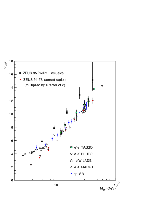
Figure 2. Figure taken from [5] showing the mean charged particle multiplicity in DIS events plotted as a function of $M_{\text{eff}}$ and confronted with the same quantity measured for other processes. The inner bars show the statistical errors, the outer ones show the statistical and systematic errors added in quadrature.

The study was conducted in a reduced phase space. The charged tracks and the energies were only measured in the polar angle interval $\theta_{\textsc{lab}}\!\in[20^{0};160^{0}]$, see Figure 3.

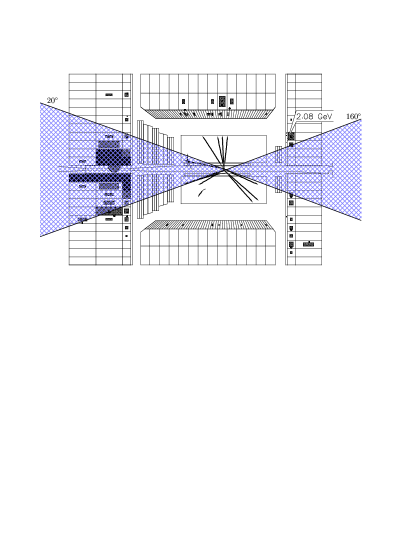
Figure 3. Typical DIS event in the ZEUS detector. The polar angle cut is shown: shaded areas are not considered in the analyses. Figure taken from [5].

This cut is justified by a large improvement in the experimental resolutions and, as proved in the same paper by means of MC simulations, it does not affect the result in any way. The other cuts are not relevant and are those normally used to obtain an almost pure set of DIS events. More details may be found in [5] or below.

Because of this cut in the polar angle, the variable $M_{\text{X}}$ is substituted with $M_{\text{eff}}$ ​: it is again a hadronic invariant mass but this time it is not the total one; in fact, it is that measured in the $\Delta\theta$ considered. Again, MC simulations proved that the dependence between $\big{<}n_{ch}\big{>}$ and $M_{\text{X}}$ ($M_{\text{eff}}$ ​​) is not affected by the phase space reduction.

From now on, unless otherwise stated, all variables refer to the reduced phase space without introducing any new notation to recall this fact. The only variable which notation will be changed is $M_{\text{X}}$ to $M_{\text{eff}}$ in order to help any comparison with [5].

Of course, the correction factor is the ratio between $A_{\text{TOT}}$ and $M_{\text{X}}$ ​ and will be denoted by $a$. This factor will be applied to the abscissa in the plot showed in Figure 2, and will be obtained in a high energy approximation: this will cause a very slight mismatch at low energies even when $A_{\text{TOT}}$ is used for re-plotting. This approximation could be avoided by re-analysing the data in terms of $A_{\text{TOT}}$ ​​.

To give an estimation of the correction factor $a$ that is suitable for our purposes, the general result (LABEL:eq:am) is useless as $\vec{p}^{\textsc{\>lead}}_{\>\textsc{tot}}$ was not measured. Also that result is strictly valid only in the full phase space. Thus the correction has been estimated by averaging over the two variables on which the said ratio depends, namely $\theta$ and $y$ (as showed below). The latter is a new variable that is defined in the next section and that expresses the unbalance in hadronic energy between the two hemispheres in a way that is suitable for our calculation.

We proceed by estimatimating the quantity $s\cdot(A_{\text{TOT}}^{2}-M^{2}_{\text{eff}})$:

$$\begin{split}s\cdot[A_{\text{TOT}}^{2}-M_{\text{eff}}^{2}]&=[E^{H}E^{I}-\vec{p}\,^{H}\vec{p}\,^{I}]^{2}-[(E^{I})^{2}-(\vec{p}\,^{I})^{2}][(E^{H})^{2}-(\vec{p}\,^{H})^{2}]=\\[11.38109pt] &=(E^{H}E^{I})^{2}+(p^{H}p^{I}\cos\theta)^{2}-2E^{H}E^{I}p^{H}p^{I}\cos\theta-\\[5.69054pt] &\qquad-(E^{H}E^{I})^{2}-(p^{I}p^{H})^{2}+(E^{I}p^{H})^{2}+(E^{H}p^{I})^{2}=\\[11.38109pt] &=(p^{H}p^{I})^{2}(\cos^{2}\theta-1)-2(E^{H}E^{I}p^{H}p^{I})\cos\theta+\\[5.69054pt] &\qquad+(E^{I}p^{H})^{2}+(E^{H}p^{I})^{2}=\ldots\end{split}\vspace*{-3mm}$$ (22)

where the index tot has been suppressed and the absolute value of 3-vectors is denoted by suppressing the arrow above the vectors.

Of course $\theta$ is the angle between $\vec{p}\,^{I}$ and $\vec{p}\,^{H}$ that is, considering HERA kinematics, between $\vec{p}\,^{H}$ and the $z$ axis:

$$\theta=\angle\>(\vec{p}\,^{H}_{T}\,;\,\hat{z})$$ (23)

This means that $\theta$ is the polar angle, and will be identified with it from now on. Introducing the high energies approximation:

$$\begin{cases}p^{H}\!\simeq E^{H}\\ p^{\,I}\simeq E^{I}\end{cases}$$

and substituting in (22) we get:

$$\begin{split}\ldots&=(E^{H}E^{I})^{2}(\cos^{2}\theta-1)-2(E^{H}E^{I})^{2}\cos\theta+2(E^{H}E^{I})^{2}=\\[11.38109pt] &=(E^{H}E^{I})^{2}(1-2\cos\theta+\cos^{2}\theta)=\\[11.38109pt] &=[E^{H}E^{I}(1-\cos\theta)]^{2}\end{split}$$ (22 ^′)

To sum up:

$$s\cdot[A_{TOT}^{2}-M_{\textrm{eff}}^{2}]\ \simeq\ [E^{H}E^{I}(1-\cos\theta)]^{2}\ \ \ \ \ \quad(E^{H,I}\simeq p^{H,I})$$ (24)

In order to further simplify the last expression we are now forced to choose a reference frame. Again the best choice is the CMS, both to simplify $s$ and for sake of visualization. Besides, it is in general the most “balanced” system, and this helps in avoiding as many troubles as possible with the high energies approximation. The only complication induced by this choice is that it forces to perform the needed transformations on data collected in the lab system.

Calculating in the CMS we obtain:

$$s\cdot[A_{\text{TOT}}^{2}-M_{\text{eff}}^{2}]\ \simeq\ (E^{H})^{2}_{\textsc{cms}}(E^{I})^{2}_{\textsc{cms}}(1-\cos\theta)^{2}_{\textsc{cms}}$$ (25)

and using

$$s=(E^{\textsc{inc}}_{\textsc{tot}})^{2}_{\textsc{cms}}$$ (26)

it becomes

$$[A_{\text{TOT}}^{2}-M_{\text{eff}}^{2}]\simeq(E^{H})^{2}_{\textsc{cms}}(1-\cos\theta)^{2}_{\textsc{cms}}$$ (27)

As already mentioned, the ratio between $A_{\text{TOT}}$ and $M_{\text{X}}$ is a function of two variables: $\Delta\theta$ and $y$. This means that, after having imposed the cuts used in the paper to be corrected, considering the collision parameter at HERA, and finally averaging over these two variables, we are left with a linear dependence of $A_{\text{TOT}}$ from $M_{\text{eff}}$ ​:

$$A_{\text{TOT}}\ \propto\ M_{\text{eff}}\qquad\text{(fixed kinematical conditions)}$$ (28)

Thus, if in general we have

$$\frac{A_{\text{TOT}}}{M_{\text{eff}}}\equiv a(\Delta\theta,y)$$ (29)

the previous remark allows the calculation of the constant $a=\big{<}a(\Delta\theta,y)\big{>}_{(\Delta\theta,y)}$ that expresses the ratio between $A_{\text{TOT}}$ and $M_{\text{X}}$ at fixed kinematical conditions:

$$a\;\equiv\;\big{<}a(\Delta\theta,y)\big{>}_{(\Delta\theta,y)}\qquad\text{(fixed kinematical conditions)}$$ (30)

Note that $a$ is invariant being the ratio between two invariants.

The dependence of $a$ from $\Delta\theta$ and $y$ will be used later to show how it is possible to obtain a different value for $a$ by tuning these parameters. This fact supports the correctness of the introduction of $A_{\text{TOT}}$ ​, as we obtain a value that allows DIS data to match with other processes curves if and only if the cuts used in [5] are taken into account.

Using the notation introduced in (29), equation (27) can be rewritten as:

$$[a^{2}(\Delta\theta,y)-1]\cdot M^{2}_{\textrm{eff}}\;\simeq\;(E^{H})^{2}_{\textsc{cms}}(1-\cos\theta)^{2}_{\textsc{cms}}$$ (27 ^′)

or, isolating $a$,

$$a^{2}(\Delta\theta,y)\;\simeq\;1+\frac{(E^{H})^{2}_{\textsc{cms}}}{M^{2}_{\textrm{eff}}}\cdot(1-\cos\theta)^{2}_{\textsc{cms}}$$ (31)

The relevant cuts and numerical values are:

• $\theta_{\textsc{lab}}\in[20^{0};160^{0}]$: the already mentioned polar angle cut [5]. It must be re-evaluated in the cms;

• $(E^{\prime}_{e})^{\textsc{lab}}_{\textsc{min}}=8\ \text{Gev}$, where the prime is used to refer to the final state and the “$e\,$” indicates the final state positron (this cut is imposed to guarantee an almost pure level of DIS events). Even this value must be re-evaluated in the cms;

• $\beta_{\textsc{boost}}$ = 0.935 is the value of the boost between the lab and the cms at HERA.

and we are now ready to estimate the correction factor we are seeking, that is, the mean of $a$ with respect to the variables it depends on:

$$a\;\equiv\;\sqrt{1+\frac{\big{<}(1-\cos\theta)^{2}_{\textsc{cms}}\big{>}\phantom{2}}{\big{<}M_{\textrm{eff}}/(E^{H}_{T})_{\textsc{cms}}\big{>}^{2}}}$$ (32)

6.1. Average over the polar angle

In this subsection only a prime is used to indicate cms variables while unprimed varibles refer to the lab system. Writing the appropriate transformations for the 4-momenta

$$\begin{cases}E^{\prime}=\gamma(E-\beta p_{z})\\[5.69054pt] p^{\prime}_{z}=\gamma(p_{z}-\beta E)\end{cases}$$ (33)

and using again the high energies approximation in the form

$$\begin{cases}p_{z}=p\cos\theta\simeq E\cos\theta\\[5.69054pt] p^{\prime}_{z}=p^{\prime}\cos\theta^{\prime}\simeq E^{\prime}\cos\theta^{\prime}\end{cases}$$ (34)

we get

$$\begin{cases}E^{\prime}=\gamma(E-\beta E\cos\theta)\\[5.69054pt] E^{\prime}\cos\theta^{\prime}=\gamma(E\cos\theta-\beta E)\end{cases}$$ (35)

so that

$$\cos\theta^{\prime}\simeq\frac{\gamma E(\cos\theta-\beta)}{\gamma E(1-\beta\cos\theta)}=\frac{\cos\theta-\beta}{1-\beta\cos\theta}$$ (36)

that is the well known formula for the aberration of light. The use of the last result is again cause of some overestimation of $a$ at low energies.

Working in the cms allows to perform the mean over the polar angle by simply averaging over the distribution obtained in (31) as, if the sample is large enough, $\big{<}\theta\big{>}_{\textsc{cms}}\simeq\,\pi/2$ .

Using the interval given in [5], ​$\theta\in[20^{0};160^{0}]$, and performing the needed transformations we get

$$\begin{cases}20^{0}&\longrightarrow\leavevmode\nobreak\ 87.895^{0}\leavevmode\nobreak\ \leavevmode\nobreak\ \>=\leavevmode\nobreak\ 1.536\leavevmode\nobreak\ \text{rad}\\[5.69054pt] 160^{0}&\longrightarrow\leavevmode\nobreak\ 176.305^{0}\leavevmode\nobreak\ =\leavevmode\nobreak\ 3.077\leavevmode\nobreak\ \text{rad.}\end{cases}$$ (37)

These are the extremes of integration to be used. The integral yields

$$\big{<}(1-\cos\theta)^{2}\big{>}_{\textsc{cms}}\>=\>\frac{{\displaystyle\int_{1.536}^{3.077}(1-\cos\theta)^{2}\mathrm{d}\theta}}{\Delta\theta}\>\simeq\>2.68$$ (38)

so that

$$a(y)\>\equiv\>\big{<}\,a(\Delta\theta,y)\,\big{>}_{(\Delta\theta)}\>\simeq\>\sqrt{1+\frac{2.68}{(M_{\text{eff}}/E^{H})^{2}}}$$ (39)

6.2. Average over the new unbalance variable “$y$”

As anticipated above, we now define a variable that suitably represents the unbalance in hadronic energy between the two hemispheres. We call this variable $y$ and define it as follows:

$$\begin{cases}E^{H}_{1,p}=y\cdot E^{H}_{T}\\[5.69054pt] E^{H}_{2,e}=(1-y)\cdot E^{H}_{T}\end{cases}$$ (40)

that is, $y$ is the fraction of hadronic energy measured in hemisphere 1 (that of the “target region”, where the proton remnant is detected).

Using $y$ we can express $M_{\text{X}}$ as a function of $E^{\textsc{had}}_{\textsc{tot}}$ in a very useful way. In fact, assuming that $\hat{k}\,^{H}_{1}\simeq-\hat{k}\,^{H}_{2}$ (where $\hat{k}\,^{H}$ represents the hadronic 3-momentum versor) we have

$$\begin{split}M_{\text{X}}\equiv\sqrt{(q_{\textsc{tot}}^{\textsc{had}})^{2}}&=\big{[}(q^{H}_{1})^{2}+(q^{H}_{2})^{2}+2E^{H}_{1}E^{H}_{2}-2\vec{p}\,^{H}_{1}\cdot\vec{p}\,^{H}_{2}\big{]}^{1/2}\simeq\\[5.69054pt] &\simeq\big{[}2E^{H}_{1}E^{H}_{2}+2E^{H}_{1}E^{H}_{2}\big{]}^{1/2}=2\sqrt{E^{H}_{1}E^{H}_{2}}\end{split}$$ (41)

that together with definition (40) yields

$$M_{\text{X}}\simeq 2\sqrt{E^{H}_{1}E^{H}_{2}}=2E^{\textsc{had}}_{\textsc{tot}}\sqrt{y(1-y)}$$ (42)

We remark that this rescaling method is applicable only if we have no more than 2 hadronic jets. In case of 3 or more jets, another method should be used or a direct data analysis must be performed.

The hadronic energies we are considering are “real” hadronic energies, that is, the energies effectively produced at the interaction vertex, regardless of the cuts applied to perform the analysis.

This does not create problems in case of a phase space reduction as there is no dependence of $M_{\text{X}}$ ($E^{\textsc{had}}_{\textsc{tot}}$ ​​) from the phase space [5]. On the contrary, the cut in the final positron energy must be considered, as the events that do not meet this condition do not become part of the statistics.

As $\big{<}y\big{>}_{\textsc{cms}\,}=1/2$  holds, for the same reason exposed in the previous section, it is sufficient to calculate the mean of the distribution obtained in the (42). Had there been no cuts in the leading particles energy, this integral would have yielded $\pi/8$, that is half the area of a circle of radius 1/2. This is not our case and we will have to take into account the relevant cuts, one of which has been already mentioned and is:

$$(E^{\prime}_{e})^{\textsc{lab}}_{\textsc{min}}=8\>\text{Gev}$$

that, as usual, must be re-evaluated in the cms:

$$\begin{split}(E^{\prime}_{e})^{\textsc{cms}}_{\textsc{min}}\>&=\>\gamma\big{[}(E^{\prime}_{e})^{\textsc{lab}}_{\textsc{min}}-\vec{\beta}\cdot\vec{p}\,^{\textsc{lab}}_{z}\big{]}\>\simeq\>(E^{\prime}_{e})^{\textsc{lab}}_{\textsc{min}}\cdot\frac{1+\beta}{\sqrt{1-\beta^{2}}}\>=\\[5.69054pt] &=(E^{\prime}_{e})^{\textsc{lab}}_{\textsc{min}}\cdot\sqrt{\frac{1+\beta}{1-\beta}}\>\simeq\>5.467\>(E^{\prime}_{e})^{\textsc{lab}}_{\textsc{min}}\>\simeq\>43.7\leavevmode\nobreak\ \text{Gev}\end{split}$$ (43)

where we have:

• considered that $\hat{\beta}$ e $\hat{z}$ are antiparallel, from where the change in sign at the second equality

• used the high energy approximation and the strong collinearity of the $e^{+}_{\textsc{out}}$ (again at the second equality)

• used the value of $\beta_{\textsc{boost}}$ for $\beta$

The highest leading longitudinal momentum in the target region is detected when a proton takes the role of the leading particle: as this maximum value, we use that representing the limit between the leading physics and the diffractive physics (in the sense described in [1] or [6]), namely:

$$(E^{\textsc{lead}}_{1,p})_{\textsc{max}}\>=\>(x_{F})_{\textsc{max}}^{\textsc{cms}}\cdot E^{\textsc{inc}}_{1,p}\>=\>0.8\>E^{\textsc{inc}}_{1,p}$$ (44)

where $x_{F}$ is the Feynman variable that represents, in practice, the fractional longitudinal momentum of the leading particle.

It should be noted that the relation between energies or momenta expressed in fractional terms are approximately invariant. In fact:

$$\begin{split}&\begin{cases}E^{\prime}_{\textsc{lead}}=\gamma(E^{L}-\vec{\beta}\cdot\vec{p}\,^{L})\\[11.38109pt] E^{\prime}_{\textsc{inc}}=\gamma(E^{I}-\vec{\beta}\cdot\vec{p}\,^{I})\end{cases}\longrightarrow\\[11.38109pt] &\longrightarrow\leavevmode\nobreak\ \leavevmode\nobreak\ \frac{E^{\prime}_{L}}{E^{\prime}_{I}}=\frac{\gamma(E^{L}-\vec{\beta}\cdot\vec{p}\,^{L})}{\gamma(E^{I}-\vec{\beta}\cdot\vec{p}\,^{I})}\simeq\frac{\gamma(1-\beta)}{\gamma(1-\beta)}\cdot\frac{E^{L}}{E^{I}}=\frac{E^{L}}{E^{I}}\end{split}$$ (45)

so that the energy of a particle expressed with the Feynman variable is about the same in two different frames at high energies and in a collinear approximation. The leading particle, as such, respects these approximations.

The two values just obtained allow to find the largest interval in hadronic energy compatible with the cuts:

$$\begin{cases}(E^{H}_{1})_{\textsc{min}}^{\textsc{cms}}={\displaystyle\frac{\sqrt{s}}{2}-\frac{4}{5}\cdot\frac{\sqrt{s}}{2}}\>\simeq\>30.0\>\text{Gev}\\[11.38109pt] (E^{H}_{2})_{\textsc{max}}^{\textsc{cms}}={\displaystyle\frac{\sqrt{s}}{2}-(E^{\prime}_{e})^{\textsc{cms}}_{\textsc{min}}}\>\simeq\>106.5\>\text{Gev}\end{cases}$$

from which the minimum for $y$ immediately follows:

$$y_{\textsc{min}}=\frac{(E^{H}_{1})_{\textsc{cms}}^{\textsc{min}}}{(E^{H}_{1})_{\textsc{cms}}^{\textsc{min}}+(E^{H}_{2})_{\textsc{cms}}^{\textsc{max}}}\simeq 0.220$$ (46)

In order to give an estimation for $y_{\textsc{max}}$, it is necessary to make some assumptions regarding $x_{F}^{\textsc{min}}$ and $(E^{\prime}_{e})^{\textsc{cms}}_{\textsc{max}}$ . A good choice, in view of a comparison with ISR data, is to adopt the same value of $x_{F}^{\textsc{min}}$ chosen at ISR, namely 0.4 :

$$(x_{F})_{\textsc{min}}^{\textsc{cms}}=0.4\>E^{\textsc{inc}}_{1,p}$$

It will also be assumed that the final state positron loses at least the 30% of its energy, value above which the diffractive events begin to prevail over the DIS ones:

$$(E^{\prime}_{e})^{\textsc{cms}}_{\textsc{max}}=0.7{\displaystyle\frac{\sqrt{s}}{2}}\>\simeq\>105\>\text{Gev}$$

From the previous two equations we get

$$\begin{cases}(E^{H}_{1})_{\textsc{cms}}^{\textsc{max}}={\displaystyle\frac{3}{5}\cdot\frac{\sqrt{s}}{2}}\>\simeq\>90.1\>\text{Gev}\\[11.38109pt] (E^{H}_{2})_{\textsc{cms}}^{\textsc{min}}={\displaystyle\frac{\sqrt{s}}{2}-(E^{\prime}_{e})^{\textsc{cms}}_{\textsc{max}}}\>\simeq\>45.0\>\text{Gev}\end{cases}$$ (47)

that in turn yields

$$y_{\textsc{max}}=\frac{(E^{H}_{1})_{\textsc{cms}}^{\textsc{max}}}{(E^{H}_{1})_{\textsc{cms}}^{\textsc{max}}+(E^{H}_{2})_{\textsc{cms}}^{\textsc{min}}}\simeq 0.667$$ (48)

Summarizing:

$$\begin{cases}y_{\textsc{min}}={\displaystyle\frac{(E^{H}_{1})_{\textsc{cms}}^{\textsc{min}}}{(E^{H}_{1})_{\textsc{cms}}^{\textsc{min}}+(E^{H}_{2})_{\textsc{cms}}^{\textsc{max}}}}\simeq 0.220\\[11.38109pt] y_{\textsc{max}}={\displaystyle\frac{(E^{H}_{1})_{\textsc{cms}}^{\textsc{max}}}{(E^{H}_{1})_{\textsc{cms}}^{\textsc{max}}+(E^{H}_{2})_{\textsc{cms}}^{\textsc{min}}}}\simeq 0.667\end{cases}$$ (49)

and it is now possible to give a numerical estimation for the mean of the distribution in hadronic energy $a$ depends on:

$$\big{<}\sqrt{y(1-y)}\>\big{>}_{\textsc{cms}}^{\textsc{hera}}=\>\frac{{\displaystyle\int_{0.220}^{0.667}\sqrt{y(1-y)}\>\mathrm{d}y}}{0.667-0.220}\>\>\simeq\>0.48\leavevmode\nobreak\ \leavevmode\nobreak\ \text{(cuts considered)}$$ (50)

or, in our case,

$$\big{<}M_{\text{X}}\big{>}_{\textsc{cms}}^{\textsc{hera}}\>=\>2E^{\textsc{had}}_{\textsc{tot}}\cdot\big{<}\sqrt{y(1-y)}\>\big{>}_{\textsc{cms}}^{\textsc{hera}}\>\simeq\>0.96\cdot E^{\textsc{had}}_{\textsc{tot}}$$ (51)

7. Final result

Given the previous results and considerations, we obtain the following correction factor $a$ to be applied in abscissa in [5]:

$$a\>\equiv\>\sqrt{1+\frac{\big{<}(1-\cos\theta)^{2}_{\textsc{cms}}\big{>}}{\big{<}M_{\textrm{eff}}/(E^{H}_{T})_{\textsc{cms}}\big{>}^{2}}}\>=\>\sqrt{1+\frac{2.68}{(0.96)^{2}}}\>=\>1.98$$ (52)

So, the plot will be showing the $\big{<}n_{ch}\big{>}$ vs $A_{\text{TOT}}$ dependence if we multiply DIS data abscissas by a factor $a$= 1.98. We recall once more that $e^{+}e^{-}$ data do not necessitate any rescaling while for $p\mspace{2.0mu}$-$p$ data an estimation of the correction factor is given below, but we can anticipate that it is negligible. The result is showed in Figure 4.

It is evident that, particularly at high energies, DIS data and other processes data follow the same curve. The quantity $\big{<}n_{ch}\big{>}$ is again a Universality Feature.

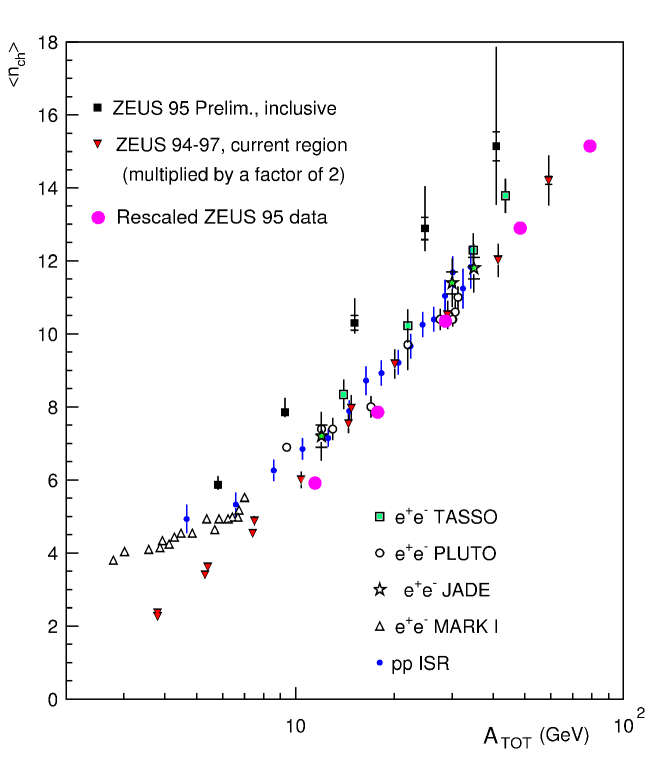
Figure 4. The same figure as 2 but with DIS data (ZEUS 95) rescaled by the factor $a\simeq 2$ and plotted in violet: now the X-axis variable is $A_{\text{TOT}}$ ​​. The universality of $\big{<}n_{ch}\big{>}$ is evident, particularly at high energies ($a$ being an asymptotic value).

8. $p\mspace{2.0mu}$-$p$ data rescaling

Recalling that the ISR was balanced and that the full phase space was considered, we can conclude that the analyses performed using $E^{\textsc{had}}_{\textsc{tot}}$ (the almost totality) were automatically made in terms of $A_{\text{TOT}}$ (see equation 11). This means that those works do not necessitate any correction.

On the contrary, in some other works, the variable $M_{\text{X}}$ was employed [6, 13, 14, 17]: these do need to be corrected for the reasons exposed in the introductory section. This may seem in contrast with the fact that no differences were found at that time when data were analysed both with $E^{\textsc{had}}_{\textsc{tot}}$ and $M_{\text{X}}$ but it is not so, the reason being in the low precisions and energies then achievable.

As an example, we estimate the difference between $A_{\text{TOT}}$ and $M_{\text{X}}$ that could have been revealed in the early works at ISR where the only condition was the presence of a leading proton leaving the vertex with

$$x_{\text{F}}\in[0.4\>,\>0.8]$$ (53)

from which it follows that

$$E^{\textsc{had}}_{\textsc{max}}\>\simeq\>3\,E^{\textsc{had}}_{\textsc{min}}$$ (54)

and this in turn allows to get the maximum value of $a$ in the “worst” situation:

$$\begin{split}\frac{A_{\text{TOT}}}{M_{\textrm{X}}}&=\frac{(E^{\textsc{had}}_{\textsc{tot}})_{\textsc{cms,lab}}}{M_{\textrm{X}}}\simeq\leavevmode\nobreak\ \leavevmode\nobreak\ \leavevmode\nobreak\ \leavevmode\nobreak\ \leavevmode\nobreak\ \leavevmode\nobreak\ \leavevmode\nobreak\ \text{(``worst'' situation)}\\[5.69054pt] &\simeq\frac{E^{\textsc{had}}_{\textsc{max}}+E^{\textsc{had}}_{\textsc{min}}}{2\sqrt{E^{\textsc{had}}_{\textsc{max}}E^{\textsc{had}}_{\textsc{min}}}}\simeq\frac{4\,E^{\textsc{had}}_{\textsc{min}}}{2\sqrt{3(E^{\textsc{had}}_{\textsc{min}})^{2}}}=\frac{2}{\sqrt{3}}\simeq 1.155\end{split}$$ (55)

where again the high energies approximation has been used in the second step. Thus, in a single event and in the worst situation, the difference between $A_{\text{TOT}}$ and $M_{\text{X}}$ could had been as large as 15%, but this is a limiting event; when averaging over all the events the difference becomes $\ll$ 15% and is consequently hidden by the large uncertainties that affected $\big{<}n_{ch}\big{>}$ at those times. It is therefore possible to safely employ ISR $p\mspace{2.0mu}$-$p$ data analysed in terms of $M_{\text{X}}$ to make a comparison with other processes data if a very high precision is not required.

9. Dependence of $a$ on $\Delta\theta\>$ and $\Delta y$

In this last section the dependence of $a$ on $\Delta\theta\>$ and $\Delta y$ is discussed with the main purpose of showing how it is improbable for the result obtained in this paper to be fortuitous.

In fact, changing kinematical conditions (using other values for $\Delta\theta$ and for $\Delta y$) would bring to different values of $a$ and the agreement between $e^{+}e^{-}$ ​​, $p\mspace{2.0mu}$-$p$ and DIS achieved in this paper could have not been obtained without taking a full account of the correct kinematical conditions.

Equation (31) shows that $a$ increases with $\theta$ and decreases with the width of the interval in $y$ (centered at 0.5). We examine the situations when $a$ is as high or as low as possible. We also check what happens in case of no phase space reduction.

It is of course safer to vary $\Delta\theta\>$ than $\Delta y$ as from the latter depends the purity of the DIS sample. Only safe values for the minimum and the maximum of $y$ will be considered.

A maximum for $2\big{<}\sqrt{y(1-y)}\>\big{>}$ is obtained by selecting a sample of balanced events:

$$y=\frac{1}{2}\leavevmode\nobreak\ \longrightarrow\leavevmode\nobreak\ 2\big{<}\sqrt{y(1-y)}\>\big{>}_{\textsc{max}}\>=\>1$$ (56)

while unbalanced events induce a minimum for $a$. If events with a fast leading proton and a low energy outgoing positron are chosen (events unbalanced in $E^{H}$ towards hemisphere 2)

$$\begin{cases}x_{F}\in[0.6\,;\,0.8]\\[11.38109pt] (E^{\prime}_{e})^{\textsc{cms}}_{\textsc{min}}\in[43,7\,;\,70]\leavevmode\nobreak\ \text{Gev}\end{cases}$$ (57)

then, in the same way used earlier, we get:

$$\begin{cases}y_{\textsc{min}}=0.220\\[5.69054pt] y_{\textsc{max}}=0.431\end{cases}$$ (58)

from which

$$\big{<}\sqrt{y(1-y)}\>\big{>}_{\textsc{min}}\>=\>0.464$$ (59)

a value that may be used to re-evaluate $a$ under modified conditions. As showed in (18 ^′) the analytical minimum for $a$ is 1:

$$a\equiv\frac{A_{\text{TOT}}}{M_{\text{eff}}}\leq 1$$ (60)

but it is not possible to reach this value in true experiments as measurements should be performed in very small and collinear intervals in $\theta\>$ (say $\theta_{\textsc{lab}}\in[0^{0};5^{0}]$). Perhaps, a realistic possibility could be $\theta_{\textsc{cms}}\!\in\![0^{0};90^{0}]$ that is $\theta_{\textsc{lab}}\!\in\![0^{0};20^{0}]$ (a choice that implies a poor resolution anyway). In such a case

$$\big{<}(1-\cos\theta)^{2}_{\textsc{cms}}\big{>}\simeq 0.23$$ (61)

which yields

$$a_{\textsc{min}}\simeq\sqrt{1+\frac{0.23}{1}}\simeq 1.1$$ (62)

that is, in these conditions $A_{\text{TOT}}$ and $M_{\text{X}}$ would be undistinguishable in practice, again because of poor resolutions. Such a study would have never been able to reveal any difference between $A_{\text{TOT}}$ and $M_{\text{eff}}$ and the universality features would have been evident even using $M_{\text{eff}}$ as it happened in some previous experiments.

In order to get much greater values for $a$ than that obtained in this work, we should go to the other side of the polar angle range, imposing, for example, $\theta_{\textsc{cms}}\in[150^{0};180^{0}]$. But this would mean to say $\theta_{\textsc{lab}}\in[174^{0};180^{0}]$, again a ridiculous interval. We are thus forced to conclude that

$$a_{\textsc{max}}\gtrsim 2\leavevmode\nobreak\ \leavevmode\nobreak\ \leavevmode\nobreak\ (\text{using }\big{<}\sqrt{y(1-y)}\>\big{>}_{\textsc{min}}\>=\>0.464)$$ (63)

and note that this study has already been performed in in a kinematical region where $a$ reachs or is very near to its maximum.

Finally, it is interesting to see what would have been obtained by working in the full phase space. Imposing

$$\Delta\theta_{\textsc{lab}}=\Delta\theta_{\textsc{cms}}=[0^{0};180^{0}]$$ (64)

we get

$$\big{<}(1-\cos\theta)^{2}_{\textsc{cms}}\big{>}=1.5$$ (65)

so that

$$a_{\textsc{(full phase space)}}=\sqrt{1+\frac{1.5}{(0.96)^{2}}}\simeq 1.62$$ (66)

a factor implying a difference that is about 40% smaller than what has been found in the reduced phase space. This result, combined with the worse resolution at the two ends of the ZEUS calorimeter, shows that a full phase space study would have been loosely able to reveal that smaller difference between $A_{\text{TOT}}$ and $M_{\text{X}}$ ​.

This discussion shows how the value estimated for $a$ and the consequent gathering toward the same curve of data points related to different processes, has a quite pronounced dependence from the “contour” conditions. As an example, using $a_{\textsc{(full phase space)}}$ to rescale DIS points in Fig. 4, would keep the mismatch between DIS and other data points evident.

This implies that a possible fortuitousness of the agreement obtained can be regarded as quite unlikely. It is of course necessary to perform direct analyses to check if $A_{\text{TOT}}$ works well in different conditions and kinds of experiments, particularly in those involving the indirect leading effect: these processes in particular appear to be the best candidates to check the geometrical justification for introducing $A_{\text{TOT}}$ ​.

10. Conclusions

After reconsidering under the correct geometrical viewpoint the kinematics of the leading effect, a new invariant has been introduced. It is likely to be the universal Lorentz-invariant quantity effectively available to multiparticle production and, as such, the variable that correctly describes the hadronization processes in any kind of particle collisions. Consequently, it has been called the Total available quadri-scalar and denoted with $A_{\text{TOT}}$ ​.

The universality of $\big{<}n_{ch}\big{>}$ has thus been recovered after that other works [5] had claimed its non-universality when comparing DIS with other kinds of processes and analysing in terms of the invariant hadronic mass $M_{\text{X}}$ ​​.

This result definitely rules out $M_{\text{X}}$ as the quantity representing the so-called “hadronic energy” and supports $A_{\text{TOT}}$ as its most reasonable successor. In order to exclude other yet-to-be-proposed possibilities to solve the universality problem, and eventually adopt $A_{\text{TOT}}$ to study and describe available and future experimental results, further analyses concerning other physical quantities need to be performed.

Appendix A:
A comparison with the generalized parton distribution approach

Finally, I would like to make a comparison and discuss similarities and differences between this work and the generalized parton distribution (hereafter: GPD) approach to the physics of particles collisions. For a recent review on the topic see [22] and references therein. I have found some similarities in the two viewpoints, but the main difference stays: the incorrect use of invariant masses to study particles collisions in general and hadronization in particular.

Of course the GPD formalism digs deep into parton dynamics and enables to perform explicit calculations concerning exclusive processes and to study some (otherwise unaccessible) quantities like, for instance, 3-dimensional (transverse) distributions of partons inside the target hadron (see Impact Parameter Representation, Sect. 3.10 of [22]) or helicities. It allows to derive interesting information about the internal structure of hadrons as well as to calculate form factors for sub-processes whose experimental study is very difficult or even not feasible, like graviton-parton interactions or gluonic currents.

The present work is based on 4-dimensional geometrical-kinematical aspects of the collision processes and consequently distinguishes longitudinal and transverse components of involved 4-momenta, just as the GPD formalism does. This surely is a common point to both approaches but general results and, in particular, aims are quite different.

In fact the present work concerns with a different aspect of particle reactions, namely the global and inclusive properties of multi-hadronic final states, which must show a global universality as a consequence of QCD universality, as has been extensively discussed in the paper.

It does not discuss exclusive processes and does not allow to compute associated amplitudes (even though it tells which is the correct variable to use to perform such a task), but concentrates instead on inclusive features of various types of reactions. We describe the collision as a 2-step process, and this is another similarity with GPD approach, but there is a main difference: our 2 steps are “visible” in the final states: the leading particle (or target remnant) is not considered as a part of the multi-hadronic final state. After this subtraction, any feature one could think of should be the same, independently from reacting particles or nominal energies. I have showed this is indeed the case for the most essential quantity related to the study and description of global properties of final states, i.e. $\big{<}n_{ch}\big{>}$ (the mean charged particle multiplicity).

The GPD approach is unable to recover this universality, the reason being the use of invariant masses. It forces to account for different kinematics when comparing processes of different nature (see e.g. Sect. 6.5.1 of [22]), when instead there is no difference at all. There are no “diffferent kinematics”, we are simply looking at things from the wrong point of view (i.e. using the wrong variables).

The use made of invariant-mass-type quantities, like $M_{\text{X}}$ (which does not take into account the transverse contribution from the leading particle) or $W^{2}$ (which, even worse, does not take into account the leading particle at all) will never allow to correctly analyse any kind of experimental data.

Of course GPD could provide very detailed predictions, were the distinction between the leading particle and the rest of the final state implemented into the formalism. It would be very interesting to use the power of GPD to extrapolate results to areas not accessible to the experiment in order to check and extend the study of hadronization under the $A_{\text{TOT}}$ framework toward those events where the leading particle is not detectable (and thus its subtraction becomes difficult if not impossible).

At any rate, it is of fundamental importance to abandone at once – both for the reason presented here and for experimental evidences of non-universality (also presented and discussed in the paper) – the use of variables like $s$ , $M_{\text{X}}$ ​, $W^{2}$ and similar when their use is evidently improper.

I suspect that many controversial results obtained in the small-$x$ regime (where the leading effect mostly plays its role: high longitudinal momentum of the leading particle: higher subtraction), as, for instance, those cited in Section 8 of [22], could be settled were $A_{\text{TOT}}$ and related variables used to re-analyse available or new data.

If the use of $A_{\text{TOT}}$ (and its derived or derivable quantities) is to be implemented in the QCD description of both hard partonic subprocesses and the hadronization phase, I believe that the longitudinal-transverse separation-oriented GPD formalism, showing the discussed similarities with the “$A_{\text{TOT}}$ approach”, could facilitate efforts toward this scope.

References

- [1] M. Basile et al., Phys. Lett. 92B, 367 (1980)
- [2] M. Basile et al., N. Cim. 58A, N.3, 193 (1980)
- [3] M. Basile et al., Phys. Lett. 95B, N.2, 311 (1980)
- [4] M. Basile et al., Phys. Lett. 99B, N.3, 247 (1981)
-
[5]
Zeus Collaboration – Multiplicity distribution in DIS at HERA. Abstract: 892
Proceedings of the XXXth International Conference on High Energy Physics; Osaka, JAPAN (08/2000) — See: www-zeus.desy.de/physics/phch/conf/osaka_paper/QCD/multipdis.ps.gz -
[6]
The Creation of Quantum Chromo Dynamics and The Effective Energy
V. N. Gribov, G. ’t Hooft, G. Veneziano, V. F. Weisskopf – Edited by L. N. Lipatov
Jointly published by: The university of Bologna and its academy of sciences - The national institute for nuclear physics (INFN) - The italian physics society (SIF), Bologna 1998 - [7] M. Basile et al., Lett. N. Cim. 30, N.16, 487 (1981)
- [8] M. Basile et al., Lett. N. Cim. 32, N.11, 321 (1981)
- [9] M. Basile et al., N. Cim. 66A, N.2, 129 (1981)
- [10] M. Basile et al., Lett. N. Cim. 32, N.7, 210 (1981)
- [11] M. Basile et al., Lett. N. Cim. 31, N.8, 273 (1981)
- [12] M. Basile et al., Lett. N. Cim. 29, N.15, 491 (1980)
- [13] M. Basile et al., Lett. N. Cim. 41, N.9, 293 (1984)
- [14] M. Basile et al., Lett. N. Cim. 36, N.10, 303 (1983)
- [15] M. Basile et al., Lett. N. Cim. 37, N.8, 289 (1983)
-
[16]
“Evidence for leading production in gluon-induced jets”
L. Cifarelli, T. Massam, D. Migani, A. Zichichi
European Organization for Nuclear Research (1997) – CERN papers - [17] M. Basile et al., N. Cim. 67A, N.3, 244 (1982)
- [18] ZEUS Coll., M. Derrick et al., Z. Phys.C67, 93-107 (1995)
- [19] ZEUS Coll., J. Breitweg et al., Eur. Phys. J. C11, 251-270 (1999)
- [20] M. Basile et al., Phys. Lett. 99B, N.3, 247 (1981)
- [21] M. Basile et al., N. Cim. 73A, N.4, 329 (1983)
- [22] M. Diehl, Phys. Rept. 388:41-277, (2003); hep-ph/0307382