Abstract

Cosmological implications of neutrinos are reviewed. The following subjects are discussed at a different level of scrutiny: cosmological limits on neutrino mass, neutrinos and primordial nucleosynthesis, cosmological constraints on unstable neutrinos, lepton asymmetry of the universe, impact of neutrinos on cosmic microwave radiation, neutrinos and the large scale structure of the universe, neutrino oscillations in the early universe, baryo/lepto-genesis and neutrinos, neutrinos and high energy cosmic rays, and briefly some more exotic subjects: neutrino balls, mirror neutrinos, and neutrinos from large extra dimensions.

Content

1. Introduction

2. Neutrino properties.

3. Basics of cosmology.
   3.1. Basic equations and cosmological parameters.
   3.2. Thermodynamics of the early universe.
   3.3. Kinetic equations.
   3.4. Primordial nucleosynthesis.

4. Massless or light neutrinos
   4.1. Gerstein-Zeldovich limit.
   4.2. Spectral distortion of massless neutrinos.

5. Heavy neutrinos.
   5.1. Stable neutrinos, $m_{\nu_{h}}<45$ GeV.
   5.2. Stable neutrinos, $m_{\nu_{h}}>45$ GeV.

6. Neutrinos and primordial nucleosynthesis.
   6.1. Bound on the number of relativistic species.
   6.2. Massive stable neutrinos. Bounds on $m_{\nu_{\tau}}$.
   6.3. Massive unstable neutrinos.
   6.4. Right-handed neutrinos.
   6.5. Magnetic moment of neutrinos.
   6.6. Neutrinos, light scalars, and BBN.
   6.7. Heavy sterile neutrinos: cosmological bounds and direct experiment.

7. Variation of primordial abundances and lepton asymmetry of the universe.

8. Decaying neutrinos.
   8.1. Introduction.
   8.2. Cosmic density constraints.
   8.3. Constraints on radiative decays from the spectrum of cosmic microwave background radiation.
   8.4. Cosmic electromagnetic radiation, other than CMB.

9. Angular anisotropy of CMB and neutrinos.

10. Cosmological lepton asymmetry.
    10.1. Introduction.
    10.2. Cosmological evolution of strongly degenerate neutrinos.
    10.3. Degenerate neutrinos and primordial nucleosynthesis.
    10.4. Degenerate neutrinos and large scale structure.
    11.4. Neutrino degeneracy and CMBR.

11. Neutrinos, dark matter and large scale structure of the universe.
    11.1. Normal neutrinos.
    11.2. Lepton asymmetry and large scale structure.
    11.3. Sterile neutrinos.
    11.4. Anomalous neutrino interactions and dark matter; unstable neutrinos.

12. Neutrino oscillations in the early universe.
    12.1. Neutrino oscillations in vacuum. Basic concepts.
    12.2. Matter effects. General description.
    12.3. Neutrino oscillations in cosmological plasma.
       12.3.1. A brief (and non-complete) review.
       12.3.2. Refraction index.
       12.3.3. Loss of coherence and density matrix.
       12.3.4. Kinetic equation for density matrix.
    12.4. Non-resonant oscillations.
    12.5. Resonant oscillations and generation of lepton asymmetry.
       12.5.1. Notations and equations.
       12.5.2. Solution without back-reaction.
       12.5.3. Back-reaction.
       12.5.4. Chaoticity.
    12.6. Active-active neutrino oscillations.
    12.7. Spatial fluctuations of lepton asymmetry.
    12.8. Neutrino oscillations and big bang nucleosynthesis.
    12.9. Summary.

13. Neutrino balls.

14. Mirror neutrinos.

15. Neutrinos and large extra dimensions.

16. Neutrinos and lepto/baryogenesis.

17. Cosmological neutrino background and ultra-high energy cosmic rays.

18. Conclusion.

19. References.

1 Introduction

The existence of neutrino was first proposed by Pauli in 1930 [1] as an attempt to explain the continuous energy spectrum observed in beta-decay [2] under the assumption of energy conservation. Pauli himself did not consider his solution to be a very probable one, though today such observation would be considered unambiguous proof of the existence of a new particle. That particle was named “neutrino” in 1933, by Fermi. A good, though brief description of historical events leading to $\nu$-discovery can be found in ref. [3].

The method of neutrino detection was suggested by Pontecorvo [4]. To this end he proposed the chlorine-argon reaction and discussed the possibility of registering solar neutrinos. This very difficult experiment was performed by Davies et al [5] in 1968, and marked the discovery neutrinos from the sky (solar neutrinos). The experimental discovery of neutrino was carried out by Reines and Cowan [6] in 1956, a quarter of a century after the existence of that particle was predicted.

In 1943 Sakata and Inouë [7] suggested that there might be more than one species of neutrino. Pontecorvo [8] in 1959 made a similar conjecture that neutrinos emitted in beta-decay and in muon decay might be different. This hypothesis was confirmed in 1962 by Danby et al [9], who found that neutrinos produced in muon decays could create in secondary interactions only muons but not electrons. It is established now that there are at least three different types (or flavors) of neutrinos: electronic ($\nu_{e}$), muonic ($\nu_{\mu}$), and tauonic ($\nu_{\tau}$) and their antiparticles. The combined LEP result [10] based on the measurement of the decay width of $Z^{0}$-boson gives the following number of different neutrino species: $N_{\nu}=2.993\pm 0.011$, including all neutral fermions with the normal weak coupling to $Z^{0}$ and mass below $m_{Z}/2\approx 45$ GeV.

It was proposed by Pontecorvo [11, 12] in 1957 that, in direct analogy with $(K^{0}-\bar{K}^{0})$-oscillations, neutrinos may also oscillate due to $(\bar{\nu}-\nu)$-transformation. After it was confirmed that $\nu_{e}$ and $\nu_{\mu}$ are different particles [9], Maki, Nakagawa, and Sakata [13] suggested the possibility of neutrino flavor oscillations, $\nu_{e}\leftrightarrow\nu_{\mu}$. A further extension of the oscillation space what would permit the violation of the total leptonic charge as well as violation of separate lepton flavor charges, $\nu_{e}\leftrightarrow\nu_{\mu}$ and $\nu_{e}\leftrightarrow\bar{\nu}_{\mu}$, or flavor oscillations of Majorana neutrinos was proposed by Pontecorvo and Gribov [14, 15]. Nowadays the phenomenon of neutrino oscillations attracts great attention in experimental particle physics as well as in astrophysics and cosmology. A historical review on neutrino oscillations can be found in refs. [16, 17].

Cosmological implications of neutrino physics were first considered in a paper by Alpher et al [18] who mentioned that neutrinos would be in thermal equilibrium in the early universe. The possibility that the cosmological energy density of neutrinos may be larger than the energy density of baryonic matter and the cosmological implications of this hypothesis were discussed by Pontecorvo and Smorodinskii [19]. A little later Zeldovich and Smorodinskii [20] derived the upper limit on the density of neutrinos from their gravitational action. In a seminal paper in 1966, Gerstein and Zeldovich [21] derived the cosmological upper limit on neutrino mass, see below sec. 4.1. This was done already in the frameworks of modern cosmology. Since then the interplay between neutrino physics and cosmology has been discussed in hundreds of papers, where limits on neutrino properties and the use of neutrinos in solving some cosmological problems were considered. Neutrinos could have been important in the formation of the large-scale structure (LSS) of the universe, in big bang nucleosynthesis (BBN), in anisotropies of cosmic microwave background radiation (CMBR), and some others cosmological phenomena. This is the subject of the present review. The field is so vast and the number of published papers is so large that I had to confine the material strictly to cosmological issues. Practically no astrophysical material is presented, though in many cases it is difficult to draw a strict border between the two. For the astrophysical implications of neutrino physics one can address the book [22] and a more recent review [23]. The number of publications rises so quickly (it seems, with increasing speed) that I had to rewrite already written sections several times to include recent developments. Many important papers could be and possibly are omitted involuntary but their absence in the literature list does not indicate any author’s preference. They are just “large number errors”. I tried to find old pioneering papers where essential physical mechanisms were discovered and the most recent ones, where the most accurate treatment was performed; the latter was much easier because of available astro-ph and hep-ph archives.

2 Neutrino properties.

It is well established now that neutrinos have standard weak interactions mediated by $W^{\pm}$- and $Z^{0}$-bosons in which only left-handed neutrinos participate. No other interactions of neutrinos have been registered yet. The masses of neutrinos are either small or zero. In contrast to photons and gravitons, whose vanishing masses are ensured by the principles of gauge invariance and general covariance respectively, no similar theoretical principle is known for neutrinos. They may have non-zero masses and their smallness presents a serious theoretical challenge. For reviews on physics of (possibly massive) neutrinos see e.g. the papers [24]-[30]. Direct observational bounds on neutrino masses, found kinematically, are:

$$m_{\nu_{e}}<\left\{\begin{array}[]{ll}2.8-2.5\,\,{\rm eV}&\mbox{\cite[cite]{[\@@bibref{}{weinheimer99,mnue}{}{}]}},\\ 10\,\,{\rm eV}&\mbox{(other groups, see \cite[cite]{[\@@bibref{}{pdg}{}{}]}) },\end{array}\right.$$ (3)

$$\begin{array}[]{ll}m_{\nu_{\mu}}<170{\rm keV}&\mbox{ \cite[cite]{[\@@bibref{}{mnum}{}{}]}},\end{array}$$ (5)

$$\begin{array}[]{ll}m_{\nu_{\tau}}<18{\rm MeV}&\mbox{\cite[cite]{[\@@bibref{}{mnut}{}{}]}},\end{array}$$ (7)

while cosmological upper limit on masses of light stable neutrinos is about 10 eV (see below, Sec. 4.1).

Even if neutrinos are massive, it is unknown if they have Dirac or Majorana mass. In the latter case processes with leptonic charge non-conservation are possible and from their absence on experiment, in particular, from the lower limits on the nucleus life-time with respect to neutrinoless double beta decay one can deduce an upper limit on the Majorana mass. The most stringent bound was obtained in Heidelberg-Moscow experiment [35]: $m_{\nu_{e}}<0.47$ eV; for the results of other groups see [25].

There are some experimentally observed anomalies (reviewed e.g. in refs. [24, 25]) in neutrino physics, which possibly indicate new phenomena and most naturally can be explained by neutrino oscillations. The existence of oscillations implies a non-zero mass difference between oscillating neutrino species, which in turn means that at least some of the neutrinos should be massive. Among these anomalies is the well known deficit of solar neutrinos, which has been registered by several installations: the pioneering Homestake, GALLEX, SAGE, GNO, Kamiokande and its mighty successor, Super-Kamiokande. One should also mention the first data recently announced by SNO [36] where evidence for the presence of $\nu_{\mu}$ or $\nu_{\tau}$ in the flux of solar neutrinos was given. This observation strongly supports the idea that $\nu_{e}$ is mixed with another active neutrino, though some mixing with sterile ones is not excluded. An analysis of the solar neutrino data can be found e.g. in refs. [37]-[42]. In the last two of these papers the data from SNO was also used.

The other two anomalies in neutrino physics are, first, the $\bar{\nu}_{e}$-appearance seen in LSND experiment [43] in the flux of $\bar{\nu}_{\mu}$ from $\mu^{+}$ decay at rest and $\nu_{e}$ appearance in the flux of $\nu_{\mu}$ from the $\pi^{+}$ decay in flight. In a recent publication [44] LSND-group reconfirmed their original results. The second anomaly is registered in energetic cosmic ray air showers. The ratio of $(\nu_{\mu}/\nu_{e})$-fluxes is suppressed by factor two in comparison with theoretical predictions (discussion and the list of the references can be found in [24, 25]). This effect of anomalous behavior of atmospheric neutrinos recently received very strong support from the Super-Kamiokande observations [45] which not only confirmed $\nu_{\mu}$-deficit but also discovered that the latter depends upon the zenith angle. This latest result is a very strong argument in favor of neutrino oscillations. The best fit to the oscillation parameters found in this paper for $\nu_{\mu}\leftrightarrow\nu_{\tau}$-oscillations are

$$\sin^{2}2\theta = 1$$

$$\Delta m^{2} = 2.2\,\times\,10^{-3}\,{\rm eV}^{2}$$ (8)

The earlier data did not permit distinguishing between the oscillations $\nu_{\mu}\leftrightarrow\nu_{\tau}$ and the oscillations of $\nu_{\mu}$ into a non-interacting sterile neutrino, $\nu_{s}$, but more detailed investigation gives a strong evidence against explanation of atmospheric neutrino anomaly by mixing between $\nu_{\mu}$ and $\nu_{s}$ [46].

After the SNO data [36] the explanation of the solar neutrino anomaly also disfavors dominant mixing of $\nu_{e}$ with a sterile neutrino and the mixing with $\nu_{\mu}$ or $\nu_{\tau}$ is the most probable case. The best fit to the solar neutrino anomaly [42] is provided by MSW-resonance solutions (MSW means Mikheev-Smirnov [47] and Wolfenstein [48], see sec. 12) - either LMA (large mixing angle solution):

$$\tan^{2}\theta = 4.1\,\times\,10^{-1}$$

$$\Delta m^{2} = 4.5\,\times\,10^{-5}\,{\rm eV}^{2}$$ (9)

or LOW (low mass solution):

$$\tan^{2}\theta = 7.1\,\times\,10^{-1}$$

$$\Delta m^{2} = 1.0\,\times\,10^{-7}\,{\rm eV}^{2}$$ (10)

Vacuum solution is almost equally good:

$$\tan^{2}\theta = 2.4\,\times\,10^{0}$$

$$\Delta m^{2} = 4.6\,\times\,10^{-10}\,{\rm eV}^{2}$$ (11)

Similar results are obtained in a slightly earlier paper [41].

The hypothesis that there may exist an (almost) new non-interacting sterile neutrino looks quite substantial but if all the reported neutrino anomalies indeed exist, it is impossible to describe them all, together with the limits on oscillation parameters found in plethora of other experiments, without invoking a sterile neutrino. The proposal to invoke a sterile neutrino for explanation of the total set of the observed neutrino anomalies was raised in the papers [49, 50]. An analysis of the more recent data and a list of references can be found e.g. in the paper [24]. Still with the exclusion of some pieces of the data, which may be unreliable, an interpretation in terms of three known neutrinos remains possible [51, 52]. For an earlier attempt to “satisfy everything” based on three-generation neutrino mixing scheme see e.g. ref. [53]. If, however, one admits that a sterile neutrino exists, it is quite natural to expect that there exist even three sterile ones corresponding to the known active species: $\nu_{e}$, $\nu_{\mu}$, and $\nu_{\tau}$. A simple phenomenological model for that can be realized with the neutrino mass matrix containing both Dirac and Majorana mass terms [54]. Moreover, the analysis performed in the paper [55] shows that the combined solar neutrino data are unable to determine the sterile neutrino admixture.

If neutrinos are massive, they may be unstable. Direct bounds on their life-times are very loose [10]: $\tau_{\nu_{e}}/m_{\nu_{e}}>300$ sec/eV, $\tau_{\nu_{\mu}}/m_{\nu_{\mu}}>15.4$ sec/eV, and no bound is known for $\nu_{\tau}$. Possible decay channels of a heavier neutrino, $\nu_{a}$ permitted by quantum numbers are: $\nu_{a}\rightarrow\nu_{b}\,\gamma$, $\nu_{a}\rightarrow\nu_{b}\,\nu_{c}\bar{\nu}_{c}$, and $\nu_{a}\rightarrow\nu_{b}\,e^{-}\,e^{+}$. If there exists a yet-undiscovered light (or massless) (pseudo)scalar boson $J$, for instance majoron [56] or familon [57], another decay channel is possible: $\nu_{a}\rightarrow\nu_{b}\,J$. Quite restrictive limits on different decay channels of massive neutrinos can be derived from cosmological data as discussed below.

In the standard theory neutrinos possess neither electric charge nor magnetic moment, but have an electric form-factor and their charge radius is non-zero, though negligibly small. The magnetic moment may be non-zero if right-handed neutrinos exist, for instance if they have a Dirac mass. In this case the magnetic moment should be proportional to neutrino mass and quite small [58, 59]:

$$\mu_{\nu}={3eG_{F}m_{\nu}\over 8\sqrt{2}\pi^{2}}\approx 3.2\times 10^{-19}\mu_{B}\left(m_{\nu}/{\rm eV}\right)$$ (12)

where $G_{F}=1.1664\cdot 10^{-5}{\rm GeV}^{-2}$ is the Fermi coupling constant, $e=\sqrt{4\pi\alpha}=0.303$ is the magnitude of electric charge of electron, and $\mu_{B}=e/2m_{e}$ is the Bohr magneton. In terms of the magnetic field units G=Gauss the Born magneton is equal to $\mu_{B}=5.788\cdot 10^{-15}{\rm MeV/G}$. The experimental upper limits on magnetic moments of different neutrino flavors are [10]:

$$\mu_{\nu_{e}}<1.8\times 10^{-10}\mu_{B},\,\,\,\mu_{\nu_{\mu}}<7.4\times 10^{-10}\mu_{B},\,\,\,\mu_{\nu_{\tau}}<5.4\times 10^{-7}\mu_{B}.$$ (13)

These limits are very far from simple theoretical expectations. However in more complicated theoretical models much larger values for neutrino magnetic moment are predicted, see sec. 6.5.

Right-handed neutrinos may appear not only because of the left-right transformation induced by a Dirac mass term but also if there exist direct right-handed currents. These are possible in some extensions of the standard electro-weak model. The lower limits on the mass of possible right-handed intermediate bosons are summarized in ref. [10] (page 251). They are typically around a few hundred GeV. As we will see below, cosmology gives similar or even stronger bounds.

Neutrino properties are well described by the standard electroweak theory that was finally formulated in the late 60th in the works of S. Glashow, A. Salam, and S. Weinberg. Together with quantum chromodynamics (QCD), this theory forms the so called Minimal Standard Model (MSM) of particle physics. All the existing experimental data are in good agreement with MSM, except for observed anomalies in neutrino processes. Today neutrino is the only open window to new physics in the sense that only in neutrino physics some anomalies are observed that disagree with MSM. Cosmological constraints on neutrino properties, as we see in below, are often more restrictive than direct laboratory measurements. Correspondingly, cosmology may be more sensitive to new physics than particle physics experiments.

3 Basics of cosmology.

3.1 Basic equations and cosmological parameters.

We will present here some essential cosmological facts and equations so that the paper would be self-contained. One can find details e.g. in the textbooks [60]-[65]. Throughout this review we will use the natural system of units, with $c$, $k$, and $\hbar$ each equaling 1. For conversion factors for these units see table 1 which is borrowed from ref. [66].

Table 1: Conversion factors for natural units.

$\rm s^{-1}$ $\rm cm^{-1}$ K eV amu erg g $\rm s^{-1}$ 1 $0.334{\times}10^{-10}$ $0.764{\times}10^{-11}$ $0.658{\times}10^{-15}$ $0.707{\times}10^{-24}$ $1.055{\times}10^{-27}$ $1.173{\times}10^{-48}$ $\rm cm^{-1}$ $2.998{\times}10^{10}$ 1 $0.229$ $1.973{\times}10^{-5}$ $2.118{\times}10^{-14}$ $3.161{\times}10^{-17}$ $0.352{\times}10^{-37}$ K $1.310{\times}10^{11}$ 4.369 $1$ $0.862{\times}10^{-4}$ $0.962{\times}10^{-13}$ $1.381{\times}10^{-16}$ $1.537{\times}10^{-37}$ eV $1.519{\times}10^{15}$ $0.507{\times}10^{5}$ $1.160{\times}10^{4}$ $1$ $1.074{\times}10^{-9}$ $1.602{\times}10^{-12}$ $1.783{\times}10^{-33}$ amu $1.415{\times}10^{24}$ $0.472{\times}10^{14}$ $1.081{\times}10^{13}$ $0.931{\times}10^{9}$ $1$ $1.492{\times}10^{-3}$ $1.661{\times}10^{-24}$ erg $0.948{\times}10^{27}$ $0.316{\times}10^{17}$ $0.724{\times}10^{16}$ $0.624{\times}10^{12}$ $0.670{\times}10^{3}$ 1 $1.113{\times}10^{-21}$ g $0.852{\times}10^{48}$ $2.843{\times}10^{37}$ $0.651{\times}10^{37}$ $0.561{\times}10^{33}$ $0.602{\times}10^{24}$ $0.899{\times}10^{21}$ 1

In the approximation of a homogeneous and isotropic universe, its expansion is described by the Friedman-Robertson-Walker metric:

$$ds^{2}=dt^{2}-a^{2}(t)\,{d{\vec{r}}\,^{2}\over 1+k{\vec{r}}\,^{2}/4}$$ (14)

For the homogeneous and isotropic distribution of matter the energy-momentum tensor has the form

$$T_{0}^{0} = \rho,$$

$$T_{i}^{j} = -p\delta_{i}^{j},\,\,(i,j=1,2,3)$$ (15)

where $\rho$ and $p$ are respectively energy and pressure densities. In this case the Einstein equations are reduced to the following two equations:

$$\ddot{a}=-(4\pi G/3)(\rho+3p)a$$ (16)

$${\dot{a}^{2}\over 2}-{4\pi\over 3}G\rho a^{2}=-{k\over 2}$$ (17)

where $G$ is the gravitational coupling constant, $G\equiv m^{-2}_{Pl}$, with the Planck mass equal to $m_{Pl}=1.221\cdot 10^{19}$ GeV. From equations (16) and (17) follows the covariant law of energy conservation, or better to say, variation:

$$\dot{\rho}=-3H(\rho+p)$$ (18)

where $H=\dot{a}/a$ is the Hubble parameter. The critical or closure energy density is expressed through the latter as:

$$\rho_{c}=3H^{2}/8\pi G\equiv 3H^{2}m_{Pl}^{2}/8\pi$$ (19)

$\rho=\rho_{c}$ corresponds to eq. (17) in the flat case, i.e. for $k=0$. The present-day value of the critical density is

$$\rho_{c}^{(0)}=3H_{0}^{2}m_{Pl}^{2}/8\pi=1.879\cdot 10^{-29}\,h^{2}\,{\rm g/cm}^{3}=10.54\,h^{2}\,{\rm keV/cm}^{3}\,,$$ (20)

where $h$ is the dimensionless value of the present day Hubble parameter $H_{0}$ measured in 100 km/sec/Mpc. The value of the Hubble parameter is rather poorly known, but it would be possibly safe to say that $h=0.5-1.0$ with the preferred value $0.72\pm 0.08$ [67].

The magnitude of mass or energy density in the universe, $\rho$, is usually presented in terms of the dimensionless ratio

$$\Omega=\rho/\rho_{c}$$ (21)

Inflationary theory predicts $\Omega=1$ with the accuracy $\pm 10^{-4}$ or somewhat better. Observations are most likely in agreement with this prediction, or at least do not contradict it. There are several different contributions to $\Omega$ coming from different forms of matter. The cosmic baryon budget was analyzed in refs. [68, 69]. The amount of visible baryons was estimated as $\Omega_{b}^{vis}\approx 0.003$ [68], while for the total baryonic mass fraction the following range was presented [69]:

$$\Omega_{B}=0.007\,-\,0.041$$ (22)

with the best guess $\Omega_{B}\sim 0.021$ (for $h=0.7$). The recent data on the angular distribution of cosmic microwave background radiation (relative heights of the first and second acoustic peaks) add up to the result presented, e.g., in ref. [70]:

$$\Omega_{B}h^{2}=0.022^{+0.004}_{-0.003}$$ (23)

Similar results are quoted in the works [71].

There is a significant contribution to $\Omega$ from an unknown dark or invisible matter. Most probably there are several different forms of this mysterious matter in the universe, as follows from the observations of large scale structure. The matter concentrated on galaxy cluster scales, according to classical astronomical estimates, gives:

$$\Omega_{DM}=\left\{\begin{array}[]{ll}(0.2-0.4)\pm 0.1&\mbox{\cite[cite]{[\@@bibref{}{wlf}{}{}]}},\\ 0.25\pm 0.2&\mbox{ \cite[cite]{[\@@bibref{}{rbt}{}{}]} },\end{array}\right.$$ (26)

A recent review on the different ways of determining $\Omega_{m}$ can be found in [74]; though most of measurements converge at $\Omega_{m}=0.3$, there are some indications for larger or smaller values.

It was observed in 1998 [75] through observations of high red-sift supernovae that vacuum energy density, or cosmological constant, is non-zero and contributes:

$$\Omega_{vac}=0.5-0.7$$ (27)

This result was confirmed by measurements of the position of the first acoustic peak in angular fluctuations of CMBR [76] which is sensitive to the total cosmological energy density, $\Omega_{tot}$. A combined analysis of available astronomical data can be found in recent works [77, 78, 79], where considerably more accurate values of basic cosmological parameters are presented.

The discovery of non-zero lambda-term deepened the mystery of vacuum energy, which is one of the most striking puzzles in contemporary physics - the fact that any estimated contribution to $\rho_{vac}$ is 50-100 orders of magnitude larger than the upper bound permitted by cosmology (for reviews see [80, 81, 82]). The possibility that vacuum energy is not precisely zero speaks in favor of adjustment mechanism[83]. Such mechanism would, indeed, predict that vacuum energy is compensated only with the accuracy of the order of the critical energy density, $\rho_{c}\sim m_{pl}^{2}/t^{2}$ at any epoch of the universe evolution. Moreover, the non-compensated remnant may be subject to a quite unusual equation of state or even may not be described by any equation of state at all. There are many phenomenological models with a variable cosmological ”constant” described in the literature, a list of references can be found in the review [84]. A special class of matter with the equation of state $p=w\rho$ with $-1<w<0$ has been named ”quintessence” [85]. An analysis of observational data [86] indicates that $w<-0.6$ which is compatible with simple vacuum energy, $w=-1$. Despite all the uncertainties, it seems quite probable that about half the matter in the universe is not in the form of normal elementary particles, possibly yet unknown, but in some other unusual state of matter.

To determine the expansion regime at different periods cosmological evolution one has to know the equation of state $p=p(\rho)$. Such a relation normally holds in some simple and physically interesting cases, but generally equation of state does not exist. For a gas of nonrelativistic particles the equation of state is $p=0$ (to be more precise, the pressure density is not exactly zero but $p\sim(T/m)\rho\ll\rho$). For the universe dominated by nonrelativistic matter the expansion law is quite simple if $\Omega=1$: $a(t)=a_{0}\cdot(t/t_{0})^{2/3}$. It was once believed that nonrelativistic matter dominates in the universe at sufficiently late stages, but possibly this is not true today because of a non-zero cosmological constant. Still at an earlier epoch ($z>1$) the universe was presumably dominated by non-relativistic matter.

In standard cosmology the bulk of matter was relativistic at much earlier stages. The equation of state was $p=\rho/3$ and the scale factor evolved as $a(t)\sim t^{1/2}$. Since at that time $\Omega$ was extremely close to unity, the energy density was equal to

$$\rho=\rho_{c}={3m_{Pl}^{2}\over 32\pi t^{2}}$$ (28)

For vacuum dominated energy-momentum tensor, $p=-\rho$, $\rho=const$, and the universe expands exponentially, $a(t)\sim\exp(H_{v}t)$.

Integrating equation (17) one can express the age of the universe through the current values of the cosmological parameters $H_{0}$ and $\Omega_{j}$, where sub-$j$ refers to different forms of matter with different equations of state:

$$t_{0}={1\over H_{0}}\int_{0}^{1}{dx\over\sqrt{1-\Omega_{tot}+\Omega_{m}x^{-1}+\Omega_{rel}x^{-2}+\Omega_{vac}x^{2}}}$$ (29)

where $\Omega_{m}$, $\Omega_{rel}$, and $\Omega_{vac}$ correspond respectively to the energy density of nonrelativistic matter, relativistic matter, and to the vacuum energy density (or, what is the same, to the cosmological constant); $\Omega_{tot}=\Omega_{m}+\Omega_{rel}+\Omega_{vac}$, and $H_{0}^{-1}=9.778\cdot 10^{9}h^{-1}$yr. This expression can be evidently modified if there is an additional contribution of matter with the equation of state $p=w\rho$. Normally $\Omega_{rel}\ll\Omega_{m}$ because $\rho_{rel}\sim a^{-4}$ and $\rho_{m}\sim a^{-3}$. On the other hand $\rho_{vac}=const$ and it is quite a weird coincidence that $\rho_{vac}\sim\rho_{m}$ just today. If $\Omega_{rel}$ and $\Omega_{vac}$ both vanishes, then there is a convenient expression for $t_{0}$ valid with accuracy better than 4% for $0<\Omega<2$:

$$t_{0}^{m}={9.788\cdot 10^{9}h^{-1}{\rm yr}\over 1+\sqrt{\Omega}}$$ (30)

Most probably, however, $\Omega_{tot}=1$, as predicted by inflationary cosmology and $\Omega_{vac}\neq 0$. In that case the universe age is

$$t_{0}^{lam}={6.525\cdot 10^{9}h^{-1}{\rm yr}\over\sqrt{\Omega_{vac}}}\ln\left[{1+\sqrt{\Omega_{vac}}\over\sqrt{1-\Omega_{vac}}}\right]$$ (31)

It is clear that if $\Omega_{vac}>0$, then the universe may be considerably older with the same value of $h$. These expressions for $t_{0}$ will be helpful in what follows for the derivation of cosmological bounds on neutrino mass.

The age of old globular clusters and nuclear chronology both give close values for the age of the universe [72]:

$$t_{0}=(14-15)\pm 2\,{\rm Gyr}$$ (32)

3.2 Thermodynamics of the early universe.

At early stages of cosmological evolution, particle number densities, $n$, were so large that the rates of reactions, $\Gamma\sim\sigma n$, were much higher than the rate of expansion, $H=\dot{a}/a$ (here $\sigma$ is cross-section of the relevant reactions). In that period thermodynamic equilibrium was established with a very high degree of accuracy. For a sufficiently weak and short-range interactions between particles, their distribution is represented by the well known Fermi or Bose-Einstein formulae for the ideal homogeneous gas (see e.g. the book [87]):

$$f^{(eq)}_{f,b}(p)={1\over\exp\left[(E-\mu)/T\right]\pm 1}$$ (33)

Here signs ’+’ and ’$-$’ refer to fermions and bosons respectively, $E=\sqrt{p^{2}+m^{2}}$ is the particle energy, and $\mu$ is their chemical potential. As is well known, particles and antiparticles in equilibrium have equal in magnitude but opposite in sign chemical potentials:

$$\mu+\bar{\mu}=0$$ (34)

This follows from the equilibrium condition for chemical potentials which for an arbitrary reaction $a_{1}+a_{2}+a_{3}\ldots\leftrightarrow b_{1}+b_{2}+\ldots$ has the form

$$\sum_{i}\mu_{a_{i}}=\sum_{j}\mu_{b_{j}}$$ (35)

and from the fact that particles and antiparticles can annihilate into different numbers of photons or into other neutral channels, $a+\bar{a}\rightarrow 2\gamma,\,3\gamma\,,\ldots$. In particular, the chemical potential of photons vanishes in equilibrium.

If certain particles possess a conserved charge, their chemical potential in equilibrium may be non-vanishing. It corresponds to nonzero density of this charge in plasma. Thus, plasma in equilibrium is completely defined by temperature and by a set of chemical potentials corresponding to all conserved charges. Astronomical observations indicate that the cosmological densities - of all charges - that can be measured, are very small or even zero. So in what follows we will usually assume that in equilibrium $\mu_{j}=0$, except for Sections 10, 11.2, 12.5, and 12.7, where lepton asymmetry is discussed. In out-of-equilibrium conditions some effective chemical potentials - not necessarily just those that satisfy condition (34) - may be generated if the corresponding charge is not conserved.

The number density of bosons corresponding to distribution (33) with $\mu=0$ is

$$n_{b}\equiv\sum_{s}\int{f_{b}(p)\over(2\pi)^{3}}\,d^{3}p=\left\{\begin{array}[]{ll}\zeta(3)g_{s}T^{3}/\pi^{2}\approx 0.12gT^{3},\,\,{\rm if}\,\,T>m;\\ (2\pi)^{-3/2}g_{s}(mT)^{3/2}\exp(-m/T),\,\,{\rm if}\,\,T<m.\end{array}\right.$$ (38)

Here summation is made over all spin states of the boson, $g_{s}$ is the number of this states, $\zeta(3)\approx 1.202$. In particular the number density of equilibrium photons is

$$n_{\gamma}=0.2404T^{3}=411.87(T/2.728{\rm K})^{3}\,{\rm cm}^{-3}$$ (39)

where 2.728 K is the present day temperature of the cosmic microwave background radiation (CMB).

For fermions the equilibrium number density is

$$n_{f}=\cases{{3\over 4}n_{b}\approx 0.09g_{s}T^{3},&if $T>m$;\cr n_{b}\approx(2\pi)^{-3/2}g_{s}(mT)^{3/2}\exp(-m/T),&if $T<m$.\cr}$$ (40)

The equilibrium energy density is given by:

$$\rho=\sum{1\over 2\pi^{2}}\int{\,dpp^{2}E\over\exp(E/T)\pm 1}$$ (41)

Here the summation is done over all particle species in plasma and their spin states. In the relativistic case

$$\rho_{rel}=(\pi^{2}/30)g_{*}T^{4}$$ (42)

where $g_{*}$ is the effective number of relativistic species, $g_{*}=\sum[g_{b}+(7/8)g_{f}]$, the summation is done over all species and their spin states. In particular, for photons we obtain

$$\rho_{\gamma}={\pi^{2}\over 15}T^{4}\approx 0.2615\left({T\over 2.728\,{\rm K}}\right)^{4}{{\rm eV\over cm^{3}}}\approx 4.662\cdot 10^{-34}\left({T\over 2.728K}\right)^{4}{{\rm g\over cm^{3}}}$$ (43)

The contribution of heavy particles, i.e. with $m>T$, into $\rho$ is exponentially small if the particles are in thermodynamic equilibrium:

$$\rho_{nr}=g_{s}m\left({mT\over 2\pi}\right)^{3/2}\exp\left(-{m\over T}\right)\left(1+{27T\over 8m}+\ldots\right)$$ (44)

Sometimes the total energy density is described by expression (42) with the effective $g_{*}(T)$ including contributions of all relativistic as well as non-relativistic species.

As we will see below, the equilibrium for stable particles sooner or later breaks down because their number density becomes too small to maintain the proper annihilation rate. Hence their number density drops as $a^{-3}$ and not exponentially. This ultimately leads to a dominance of massive particles in the universe. Their number and energy densities could be even higher if they possess a conserved charge and if the corresponding chemical potential is non-vanishing.

Since $\Omega_{m}$ was very close to unity at early cosmological stages, the energy density at that time was almost equal to the critical density (28). Taking this into account, it is easy to determine the dependence of temperature on time during RD-stage when $H=1/2t$ and $\rho$ is given simultaneously by eqs. (42) and (28):

$$tT^{2}=\left({90\over 32\pi^{3}}\right)^{1/2}{m_{Pl}\over\sqrt{g}_{*}}={2.42\over\sqrt{g}_{*}}\,({\rm MeV})^{2}\,{\rm sec}$$ (45)

For example, in equilibrium plasma consisting of photons, $e^{\pm}$, and three types of neutrinos with temperatures above the electron mass but below the muon mass, $0.5<T<100$ MeV, the effective number of relativistic species is

$$g_{*}=10.75$$ (46)

In the course of expansion and cooling down, $g_{*}$ decreases as the particle species with $m>T$ disappear from the plasma. For example, at $T\ll m_{e}$ when the only relativistic particles are photons and three types of neutrinos with the temperature $T_{\nu}\approx 0.71\,T_{\gamma}$ the effective number of species is

$$g_{*}=3.36$$ (47)

If all chemical potentials vanish and thermal equilibrium is maintained, the entropy of the primeval plasma is conserved:

$${d\over dt}\left(a^{3}\,{p+\rho\over T}\right)=0$$ (48)

In fact this equation is valid under somewhat weaker conditions, namely if particle occupation numbers $f_{j}$ are arbitrary functions of the ratio $E/T$ and the quantity $T$ (which coincides with temperature only in equilibrium) is a function of time subject to the condition (18).

3.3 Kinetic equations.

The universe is not stationary, it expands and cools down, and as a result thermal equilibrium is violated or even destroyed. The evolution of the particle occupation numbers $f_{j}$ is usually described by the kinetic equation in the ideal gas approximation. The latter is valid because the primeval plasma is not too dense, particle mean free path is much larger than the interaction radius so that individual distribution functions $f(E,t)$, describing particle energy spectrum, are physically meaningful. We assume that $f(E,t)$ depends neither on space point ${\vec{x}}$ nor on the direction of the particle momentum. It is fulfilled because of cosmological homogeneity and isotropy. The universe expansion is taken into account as a red-shifting of particle momenta, $\dot{p}=-Hp$. It gives:

$${df_{i}\over dt}={\partial f_{i}\over\partial t}+{\partial f_{i}\over\partial p_{i}}\dot{p}_{i}={\partial f_{i}\over\partial t}-Hp_{i}{\partial f_{i}\over\partial p_{i}}$$ (49)

As a result the kinetic equation takes the form

$$\left({\partial\over\partial t}-Hp_{i}{\partial\over\partial p_{i}}\right)f_{i}(p_{i},t)=I^{coll}_{i}$$ (50)

where $I^{coll}_{i}$ is the collision integral for the process $i+Y\leftrightarrow Z$:

$$I^{coll}_{i} = -{(2\pi)^{4}\over 2E_{i}}\sum_{Z,Y}\int\,d\nu_{Z}\,d\nu_{Y}\delta^{4}(p_{i}+p_{Y}-p_{Z})[\mid A(i+Y\rightarrow Z)\mid^{2}$$ (51)

$$f_{i}\prod_{Y}f\prod_{Z}(1\pm f)-\mid A(Z\rightarrow i+Y)\mid^{2}\prod_{Z}f\prod_{i+Y}(1\pm f)]$$

Here $Y$ and $Z$ are arbitrary, generally multi-particle states, $\prod_{Y}f$ is the product of phase space densities of particles forming the state $Y$, and

$$d\nu_{Y}=\prod_{Y}{\overline{dp}}\equiv\prod_{Y}{d^{3}p\over(2\pi)^{3}2E}$$ (52)

The signs ’+’ or ’$-$’ in $\prod(1\pm f)$ are chosen for bosons and fermions respectively.

It can be easily verified that in the stationary case ($H=0$), the distributions (33) are indeed solutions of the kinetic equation (50), if one takes into account the conservation of energy $E_{i}+\sum_{Y}E=\sum_{Z}E$, and the condition (35). This follows from the validity of the relation

$$\prod_{i+Y}f^{(eq)}\prod_{Z}(1\pm f^{(eq)})=\prod_{Z}f^{(eq)}\prod_{i+Y}(1\pm f^{(eq)})$$ (53)

and from the detailed balance condition, $\mid A(i+Y\rightarrow Z)\mid=\mid A(Z\rightarrow i+Y)\mid$ (with a trivial transformation of kinematical variables). The last condition is only true if the theory is invariant with respect to time reversion. We know, however, that CP-invariance is broken and, because of the CPT-theorem, T-invariance is also broken. Thus T-invariance is only approximate. Still even if the detailed balance condition is violated, the form of equilibrium distribution functions remain the same. This is ensured by the weaker condition [88]:

$$\sum_{k}\int\,d\nu_{Z_{k}}\delta^{4}\left(\sum_{Z_{k}}p-p_{f}\right)\left(\mid A(Z_{k}\rightarrow f)\mid^{2}-\mid A(f\rightarrow Z_{k}\mid^{2}\right)=0$$ (54)

where summation is made over all possible states $Z_{k}$. This condition can be termed the cyclic balance condition, because it demonstrates that thermal equilibrium is achieved not by a simple equality of probabilities of direct and inverse reactions but through a more complicated cycle of reactions. Equation (54) follows from the unitarity of $S$-matrix, $S^{+}S=SS^{+}=1$. In fact, a weaker condition is sufficient for saving the standard form of the equilibrium distribution functions, namely the diagonal part of the unitarity relation, $\sum_{f}W_{if}=1$, and the inverse relation $\sum_{i}W_{if}=1$, where $W_{if}$ is the probability of transition from the state $i$ to the state $f$. The premise that the sum of probabilities of all possible events is unity is of course evident. Slightly less evident is the inverse relation, which can be obtained from the first one by the CPT-theorem.

For the solution of kinetic equations, which will be considered below, it is convenient to introduce the following dimensionless variables:

$$x=m_{0}a\,\,\,{\rm and}\,\,y_{j}=p_{j}a$$ (55)

where $a(t)$ is the scale factor and $m_{0}$ is some fixed parameter with dimension of mass (or energy). Below we will take $m_{0}=1$ MeV. The scale factor $a$ is normalized so that in the early thermal equilibrium relativistic stage $a=1/T$. In terms of these variables the l.h.s. of kinetic equation (50) takes a very simple form:

$$Hx{\partial f_{i}\over\partial x}=I^{coll}_{i}$$ (56)

When the universe was dominated by relativistic matter and when the temperature dropped as $T\sim 1/a$, the Hubble parameter could be taken as

$$H=5.44\sqrt{{g_{*}\over 10.75}}\,{m_{0}^{2}\over x^{2}m_{Pl}}$$ (57)

In many interesting cases the evolution of temperature differs from the simple law specified above but still the expression (57) is sufficiently accurate.

3.4 Primordial nucleosynthesis

Primordial or big bang nucleosynthesis (BBN) is one of the cornerstones of standard big bang cosmology. Its theoretical predictions agree beautifully with observations of the abundances of the light elements, ${}^{2}H$, ${}^{3}He$, ${}^{4}He$ and ${}^{7}Li$, which span 9 orders of magnitude. Neutrinos play a significant role in BBN, and the preservation of successful predictions of BBN allows one to work our restrictive limits on neutrino properties.

Below we will present a simple pedagogical introduction to the theory of BBN and briefly discuss observational data. The content of this subsection will be used in sec. 6 for the analysis of neutrino physics at the nucleosynthesis epoch. A good reference where these issues are discussed in detail is the book [89]; see also the review papers [90, 91] and the paper [92] where BBN with degenerate neutrinos is included.

The relevant temperature interval for BBN is approximately from 1 MeV to 50 keV. In accordance with eq. (45) the corresponding time interval is from 1 sec to 300 sec. When the universe cooled down below MeV the weak reactions

$$n+\nu_{e} \leftrightarrow p+e^{-},$$ (58)

$$n+e^{+} \leftrightarrow p+\bar{\nu}$$ (59)

became slow in comparison with the universe expansion rate, so the neutron-to-proton ratio, $n/p$, froze at a constant value $(n/p)_{f}=\exp\left(-\Delta m/T_{f}\right)$, where $\Delta m=1.293$ MeV is the neutron-proton mass difference and $T_{f}=0.6-0.7$ MeV is the freezing temperature. At higher temperatures the neutron-to-proton ratio was equal to its equilibrium value, $(n/p)_{eq}=\exp(-\Delta m/T)$. Below $T_{f}$ the reactions (58) and (59) stopped and the evolution of $n/p$ is determined only by the neutron decay:

$$n\rightarrow p+e+\bar{\nu}_{e}$$ (60)

with the life-time $\tau_{n}=887\pm 2$ sec.

In fact the freezing is not an instant process and this ratio can be determined from numerical solution of kinetic equation. The latter looks simpler for the neutron to baryon ratio, $r=n/(n+p)$:

$$\dot{r}={(1+3g^{2}_{A})G_{F}^{2}\over 2\pi^{3}}\left[A-(A+B)\,r\right]$$ (61)

where $g_{A}=-1.267$ is the axial coupling constant and the coefficient functions are given by the expressions

$$A=\int^{\infty}_{0}dE_{\nu}E_{\nu}^{2}E_{e}p_{e}f_{e}(E_{e})\left[1-f_{\nu}(E_{\nu})\right]|_{E_{e}=E_{\nu}+\Delta m}+$$

$$\int_{m_{e}}^{\infty}dE_{e}E_{\nu}^{2}E_{e}p_{e}f_{\bar{\nu}}(E_{\nu})\left[1-f_{\bar{e}}(E_{e}\right]\mid_{E_{\nu}=E_{e}+\Delta m}+$$

$$\int_{m_{e}}^{\Delta m}dE_{e}E_{\nu}^{2}E_{e}p_{e}f_{\bar{\nu}}(E_{\nu})f_{e}(E_{e})\mid_{E_{\nu}+E_{e}=\Delta m}\,,$$ (62)

$$B=\int^{\infty}_{0}dE_{\nu}E_{\nu}^{2}E_{e}p_{e}f_{\nu}(E_{\nu})\left[1-f_{e}(E_{e})\right]|_{E_{e}=E_{\nu}+\Delta m}+$$

$$\int_{m_{e}}^{\infty}dE_{e}E_{\nu}^{2}E_{e}p_{e}f_{\bar{e}}(E_{e})\left[1-f_{\bar{\nu}}(E_{\nu})\right]\mid_{E_{\nu}=E_{e}+\Delta m}+$$

$$\int_{m_{e}}^{\Delta m}dE_{e}E_{\nu}^{2}E_{e}p_{e}\left[1-f_{\bar{\nu}}(E_{\nu})\right]\left[1-f_{e}(E_{e})\right]\mid_{E_{\nu}+E_{e}=\Delta m}$$ (63)

These rather long expressions are presented here because they explicitly demonstrate the impact of neutrino energy spectrum and of a possible charge asymmetry on the $n/p$-ratio. It can be easily verified that for the equilibrium distributions of electrons and neutrinos the following relation holds, $A=B\exp\left(-\Delta m/T\right)$. In the high temperature limit, when one may neglect $m_{e}$, the function $B(T)$ can be easily calculated:

$$B=48T^{5}+24(\Delta m)T^{4}+4(\Delta m)^{2}T^{3}$$ (64)

Comparing the reaction rate, $\Gamma=(1+3g^{2}_{A})G_{F}^{2}B/2\pi^{3}$ with the Hubble parameter taken from eq. (45), $H=T^{2}\sqrt{g_{*}}/0.6m_{Pl}$, we find that neutrons-proton ratio remains close to its equilibrium value for temperatures above

$$T_{np}=0.7\left({g_{*}\over 10.75}\right)^{1/6}{\rm MeV}$$ (65)

Note that the freezing temperature, $T_{np}$, depends upon $g_{*}$, i.e. upon the effective number of particle species contributing to the cosmic energy density.

The ordinary differential equation (61) can be derived from the master equation (50) either in nonrelativistic limit or, for more precise calculations, under the assumption that neutrons and protons are in kinetic equilibrium with photons and electron-positron pairs with a common temperature $T$, so that $f_{n,p}\sim\exp(-E/T)$. As we will see in what follows, this is not true for neutrinos below $T=2-3$ MeV. Due to $e^{+}e^{-}$-annihilation the temperature of neutrinos became different from the common temperature of photons, electrons, positrons, and baryons. Moreover, the energy distributions of neutrinos noticeably (at per cent level) deviate from equilibrium, but the impact of that on light element abundances is very weak (see sec. 4.2).

The matrix elements of $(n-p)$-transitions as well as phase space integrals used for the derivation of expressions (62) and (63) were taken in non-relativistic limit. One may be better off taking the exact matrix elements with finite temperature and radiative corrections to calculate the $n/p$ ratio with very good precision (see refs. [93, 94] for details). Since reactions (58) and (59) as well as neutron decay are linear with respect to baryons, their rates $\dot{n}/n$ do not depend upon the cosmic baryonic number density, $n_{B}=n_{p}+n_{n}$, which is rather poorly known. The latter is usually expressed in terms of dimensionless baryon-to-photon ratio:

$$\eta_{10}\equiv 10^{10}\eta=10^{10}n_{B}/n_{\gamma}$$ (66)

Until recently, the most precise way of determining the magnitude of $\eta$ was through the abundances of light elements, especially deuterium and ${}^{3}He$, which are very sensitive to it. Recent accurate determination of the position and height of the second acoustic peak in the angular spectrum of CMBR [70, 71] allows us to find baryonic mass fraction independently. The conclusions of both ways seem to converge around $\eta_{10}=5$.

The light element production goes through the chain of reactions: $p\,(n,\gamma)\,d$, $d\,(p\gamma)\,^{3}He$, $d\,(d,n)\,^{3}He$, $d\,(d,p)\,t$, $t\,(d,n)\,^{4}He$, etc. One might expect naively that the light nuclei became abundant at $T=O({\rm MeV})$ because a typical nuclear binding energy is several MeV or even tens MeV. However, since $\eta=n_{B}/n_{\gamma}$ is very small, the amount of produced nuclei is tiny even at temperatures much lower than their binding energy. For example, the number density of deuterium is determined in equilibrium by the equality of chemical potentials, $\mu_{d}=\mu_{p}+\mu_{n}$. From that and the expression (38) we obtain:

$$n_{d}=3e^{\left(\mu_{d}-m_{d}\right)/T}\left({m_{d}T\over 2\pi}\right)^{3/2}={3\over 4}n_{n}n_{p}e^{B/T}\left(2\pi m_{d}\over m_{p}m_{n}T\right)^{3/2}$$ (67)

where $B_{D}=2.224$ MeV is the deuterium binding energy and the coefficient 3/4 comes from spin counting factors. One can see that $n_{d}$ becomes comparable to $n_{n}$ only at the temperature:

$$T_{d}={0.064\,{\rm MeV}\over 1-0.029\ln\eta_{10}}$$ (68)

At higher temperatures deuterium number density in cosmic plasma is negligible. Correspondingly, the formation of other nuclei, which stems from collisions with deuterium is suppressed. Only deuterium could reach thermal equilibrium with protons and neutrons. This is the so called ”deuterium bottleneck”. But as soon as $T_{d}$ is reached, nucleosynthesis proceeds almost instantly. In fact, deuterium never approaches equilibrium abundance because of quick formation of heavier elements. The latter are created through two-body nuclear collisions and hence the probability of production of heavier elements increases with an increase of the baryonic number density. Correspondingly, less deuterium survives with larger $\eta$. Practically all neutrons that had existed in the cosmic plasma at $T\approx T_{d}$ were quickly captured into ${}^{4}He$. The latter has the largest binding energy, $B_{{}^{4}He}=28.3$ MeV, and in equilibrium its abundance should be the largest. Its mass fraction, $Y(^{4}He)$, is determined predominantly by the $(n/p)$-ratio at the moment when $T\approx T_{d}$ and is approximately equal to $2(n/p)/[1+(n/p)]\approx 25\%$. There is also some production of ${}^{7}Li$ at the level (a few)$\times 10^{-10}$. Heavier elements in the standard model are not produced because the baryon number density is very small and three-body collisions are practically absent.

Theoretical calculations of light elements abundances are quite accurate, given the values of the relevant parameters: neutron life-time, which is pretty well known now, the number of massless neutrino species, which equals 3 in the standard model and the ratio of baryon and photon number densities during nucleosynthesis, $\eta_{10}=10^{10}(n_{B}/n_{\gamma})$ (66). The last parameter brings the largest uncertainty into theoretical results. There are also some uncertainties in the values of the nuclear reaction rates which were never measured at such low energies in plasma environment. According to the analysis of ref. [95] these uncertainties could change the mass fraction of ${}^{4}He$ at the level of a fraction of per cent, but for deuterium the “nuclear uncertainty” is about 10% and for ${}^{7}Li$ it is could be as much as 25%. An extensive discussion of possible theoretical uncertainties and a list of relevant references can be found in recent works [93, 94]. Typical curves for primordial abundances of light elements as functions of $\eta_{10}$, calculated with the nucleosynthesis code of ref. [96], are presented in fig. 1.

Figure 1: Abundances of light elements ${}^{2}H$ (by number) ${}^{4}He$ (by mass), and ${}^{7}Li$ (by number) as functions of baryon-to-photon ratio $\eta_{10}\equiv 10^{10}n_{B}/n_{\gamma}$.

Another, and a very serious source of uncertainties, concerns the comparison of theory with observations. Theory quite precisely predicts primordial abundances of light elements, while observations deals with the present day abundances. The situation is rather safe for ${}^{4}He$ because this element is very strongly bound and is not destroyed in the course of evolution. It can only be created in stars. Thus any observation of the present-day mass fraction of ${}^{4}He$ gives an upper limit to its primordial value. To infer its primordial value $Y_{p}$, the abundance of ${}^{4}He$ is measured together with other heavier elements, like oxygen, carbon, nitrogen, etc (all they are called ”metals”) and the data is extrapolated to zero metallicity (see the book [89] for details). The primordial abundance of deuterium is very sensitive to the baryon density and could be in principle a very accurate indicator of baryons [97]. However deuterium is fragile and can be easily destroyed. Thus it is very difficult to infer its primordial abundance based on observations at relatively close quarters in the media where a large part of matter had been processed by the stars. Recently, however, it became possible to observe deuterium in metal-poor gas clouds at high red-shifts. In these clouds practically no matter was contaminated by stellar processes so these measurements are believed to yield the primordial value of $D/H$. Surprisingly, the results of these measurements are grouped around two very different values, normal deuterium, $(D/H)_{p}\approx 3\cdot 10^{-5}$ [98]-[100], which is reasonably close to what is observed in the Galaxy, and high deuterium, $(D/H)_{p}\approx(1-2)\cdot 10^{-4}$ [101]-[105]. The observed variation may not be real; for example, uncertainties in the velocity field allow the D/H ratio in the system at $z=0.7$ [105] to be as low as in the two high-z systems [106]-[108]. An interpretation of the observations in the system at $z=0.7$ under the assumption of a simple single $(H+D)$-component [107] gives $8\cdot 10^{-5}<D/H<57\cdot 10^{-5}$. With the possibility of a complicated velocity distribution or of a second component in this system a rather weak limit was obtained [107], $D/H<50\cdot 10^{-5}$. However, it was argued in the recent work [109] that the observed absorption features most probably are not induced by deuterium and thus the conclusion of anomalously high deuterium in this system might be incorrect. On the other hand, there are systems where anomalously low fraction of deuterium is observed [110], $D/H\sim(1-2)\cdot 10^{-5}$. An analysis of the data on D and ${}^{4}He$ and recent references can be found in [111]. It seems premature to extract very accurate statements about baryon density from these observations. The accuracy of the determination of light element abundances is often characterized in terms of permitted additional neutrino species, $\Delta N_{\nu}$. The safe upper limit, roughly speaking, is that one extra neutrino is permitted in addition to the known three (see sec. 6.1). On the other hand, if all observed anomalous deuterium (high or low) is not real and could be explained by some systematic errors or misinterpretation of the data and only “normal” data are correct, then BBN would provide quite restrictive upper bound on the number of additional neutrino species, $\Delta N_{\nu}<0.2$ [112]. For more detail and recent references see sec. 6.1.

4 Massless or light neutrinos

4.1 Gerstein-Zeldovich limit

Here we will consider neutrinos that are either massless or so light that they had decoupled from the primordial $e^{\pm}\,\gamma$-plasma at $T>m_{\nu}$. A crude estimate of the decoupling temperature can be obtained as follows. The rate of neutrino interactions with the plasma is given by:

$$\Gamma_{\nu}\equiv\dot{n}_{\nu}/n_{\nu}=\langle\sigma_{\nu e}n_{e}\rangle$$ (69)

where $\sigma_{\nu e}$ is the cross section of neutrino-electron scattering or annihilation and $\langle...\rangle$ means thermal averaging. Decoupling occurs when the interaction rate falls below the expansion rate, $\Gamma_{\nu}<H$. One should substitute for the the cross-section $\sigma_{\nu e}$ the sum of the cross-sections of neutrino elastic scattering on electrons and positrons and of the inverse annihilation $e^{+}e^{-}\rightarrow\bar{\nu}\nu$ in the relativistic limit. Using expressions presented in Table 2 we find:

$$\sigma_{\nu,e}={5G^{2}_{F}\,s\over 3\pi}\left(g^{2}_{L}+g^{2}_{R}\right)$$ (70)

where $s=(p_{1}+p_{2})^{2}$, $p_{1,2}$ are the 4-momenta of the initial particles, and $g_{L,R}$ are the coupling to the left-handed and right-handed currents respectively, $g_{L}=\pm 1/2+\sin^{2}\theta_{W}$ and $g_{R}=\sin^{2}\theta_{W}$, plus or minus in $g_{L}$ stand respectively for $\nu_{e}$ or $\nu_{\mu,\tau}$. The weak mixing angle $\theta_{W}$ is experimentally determined as $\sin^{2}\theta_{W}=0.23$.

	Process				$2^{-5}G^{-2}_{F}S\left|A\right|^{2}$
$\nu_{e}+\bar{\nu}_{e}$	$\rightarrow$	$\nu_{e}+\bar{\nu}_{e}$			$4(p_{1}\cdot p_{4})(p_{2}\cdot p_{3})$
$\nu_{e}+\nu_{e}$	$\rightarrow$	$\nu_{e}+\nu_{e}$			$2(p_{1}\cdot p_{2})(p_{3}\cdot p_{4})$
$\nu_{e}+\bar{\nu}_{e}$	$\rightarrow$	$\nu_{\mu(\tau)}+\bar{\nu}_{\mu(\tau)}$			$(p_{1}\cdot p_{4})(p_{2}\cdot p_{3})$
$\nu_{e}+\bar{\nu}_{\mu(\tau)}$	$\rightarrow$	$\nu_{e}+\bar{\nu}_{\mu(\tau)}$			$(p_{1}\cdot p_{4})(p_{2}\cdot p_{3})$
$\nu_{e}+\nu_{\mu(\tau)}$	$\rightarrow$	$\nu_{e}+\nu_{\mu(\tau)}$			$(p_{1}\cdot p_{2})(p_{3}\cdot p_{4})$
$\nu_{e}+\bar{\nu}_{e}$	$\rightarrow$	$e^{+}+e^{-}$			$4[(g_{L}^{2}(p_{1}\cdot p_{4})(p_{2}\cdot p_{3})$
					$+g_{R}^{2}(p_{1}\cdot p_{3})(p_{2}\cdot p_{4})$
					$+g_{L}g_{R}m_{e}^{2}(p_{1}\cdot p_{2})]$
$\nu_{e}+e^{-}$	$\rightarrow$	$\nu_{e}+e^{-}$			$4[g_{L}^{2}(p_{1}\cdot p_{2})(p_{3}\cdot p_{4})$
					$+g_{R}^{2}(p_{1}\cdot p_{4})(p_{2}\cdot p_{3})$
					$-g_{L}g_{R}m_{e}^{2}(p_{1}\cdot p_{3})]$
$\nu_{e}+e^{+}$	$\rightarrow$	$\nu_{e}+e^{+}$			$4[g_{R}^{2}(p_{1}\cdot p_{2})(p_{3}\cdot p_{4})$
					$+g_{L}^{2}(p_{1}\cdot p_{4})(p_{2}\cdot p_{3})$
					$-g_{L}g_{R}m_{e}^{2}(p_{1}\cdot p_{3})]$

Table 2: Matrix elements squared for reactions with electron neutrino; $S$ is the symmetrization factor related to identical particles in the initial or final state, $g_{L}=\frac{1}{2}+\sin^{2}\theta_{W}$ and $g_{R}=\sin^{2}\theta_{W}$. Matrix elements for muon or tau neutrino processes are obtained by the substitutions $\nu_{e}\rightarrow\nu_{\mu,\tau}$ and $g_{L}\rightarrow\tilde{g}_{L}=g_{L}-1$.

We would not proceed along these lines because one can do better by using kinetic equation (56). We will keep only direct reaction term in the collision integral and use the matrix elements taken from the Table 2. We estimate the collision integral in the Boltzmann approximation. According to calculations of ref. [113] this approximation is good with an accuracy of about 10%. We also assume that particles with which neutrinos interact, are in thermal equilibrium with temperature $T$. After straightforward calculations we obtain:

$$Hx\,{\partial f_{\nu}\over f_{\nu}\,\partial x}=-{80G_{F}^{2}\left(g_{L}^{2}+g_{R}^{2}\right)y\over 3\pi^{3}x^{5}}$$ (71)

Using the expression (57) and integrating over $x$ we find for the decoupling temperature of electronic neutrinos $T_{\nu_{e}}=2.7y^{-1/3}$ MeV and $T_{\nu_{\mu},\nu_{\tau}}=4.5y^{-1/3}$ MeV. This can be compared with the results of refs. [114, 115]. On the average one can take $\langle y\rangle=3$ and $T_{\nu_{e}}=1.87$ MeV and $T_{\nu_{\mu},\nu_{\tau}}=3.12$ MeV. These results are applicable to the decoupling of neutrinos from the electromagnetic component of the plasma, i.e. from $e^{\pm}$ and photons. If we take into account all possible reactions of neutrinos in the the plasma, including their scattering on themselves, the coefficient $(g_{L}^{2}+g_{R}^{2})$ should be changed into $(1+g_{L}^{2}+g_{R}^{2})$. These results are in agreement with refs. [115, 116] (see discussion in sec. 12.3.3). Correspondingly the decoupling temperature determined with respect to the total reaction rate would be $T_{\nu_{e}}=1.34$ MeV and $T_{\nu_{\mu},\nu_{\tau}}=1.5$ MeV. Somewhat more accurate calculations of the reaction rates with Fermi exclusion taken into account were performed in ref. [117], see eq. (319) and discussion after it. The finite temperature corrections to the reaction rates have been studied in ref. [118]. As a result of these corrections the interaction rate becomes weaker and the decoupling temperature rises by 4.4%.

The decoupling temperature depends upon neutrino momentum, so that more energetic neutrinos decouple later. In fact the decoupling temperature is somewhat higher because inverse reactions neglected in this estimate diminish the reaction rate approximately by half if the distribution is close to the equilibrium one. Anyway, it is safe to say that below 2 MeV neutrinos practically became non-interacting and their number density remains constant in a comoving volume, $n_{\nu}\sim 1/a^{3}$. At the moment of decoupling the relative number density of neutrinos was determined by thermal equilibrium and in the absence of charge asymmetry was given by:

$${n_{\nu_{j}}\over n_{\gamma}}={n_{\bar{\nu}_{j}}\over n_{\gamma}}={3\over 8}$$ (72)

Later $e^{+}e^{-}$-annihilation enlarges the number density of photons in the comoving volume. This increase can be easily calculated using the entropy conservation law (48). The photon number density increases proportionally to the ratio of the number of species before and after annihilation. In the case under consideration, it is $(2+7/2)/2=11/4$. If no more photons were created during the subsequent expansion, then the present day neutrino-to-photon ratio should be

$${n_{\nu_{j}}+n_{\bar{\nu}_{j}}\over n_{\gamma}}={3\over 11}$$ (73)

The number density of photons in CMB radiation is now known with a great degree of precision, see (39). From that we find $n_{\nu_{j}}+n_{\bar{\nu}_{j}}=112/{\rm cm^{3}}$ for any kind of light ($m<O({\rm MeV})$) neutrino. If neutrinos are massless, they preserve their initial Fermi distribution with the present day temperature $T_{\nu}=1.95$ K (although there are some deviations, which will be discussed in the next subsection). If they are massive they are much colder. Energy density of massive neutrinos is $\rho_{\nu}=112\sum_{j}m_{\nu_{j}}/{\rm cm}^{3}=\rho_{c}h^{-2}\sum_{j}\left(m_{\nu_{j}}/94{\rm eV}\right)$ Assuming that $\Omega_{\nu}=\rho_{\nu}/\rho_{c}\leq 1$ we obtain the following upper limit on neutrino masses:

$$\sum m_{\nu_{j}}<94{\rm eV}\,\,\Omega h^{2}$$ (74)

In particular for $h=0.7$ and $\Omega_{matter}<0.3$ the mass of neutrino should be smaller than 14 eV. This bound was first found by Gerstein and Zeldovich [21] and with different modifications was considered in many subsequent papers. A good account of historical developments that led to the discovery of this bound can be found in ref. [119]. That account has been marred, however, by a serious misquotation of the Gerstein and Zeldovich paper. Namely it was claimed [119] that the GZ calculations of the relic neutrino abundance was erroneous because they assumed that massive neutrinos are Dirac particles with fully populated right-handed states and that they (GZ) ”did not allow for the decrease in the neutrino temperature relative to photons due to $e^{+}e^{-}$-annihilation”. Both accusations are incorrect. It is explicitly written in GZ paper: ”In considering the question of the possible mass of the neutrino we have, naturally, used statistical formulas for four-component $m\neq 0$ particles. We know, however, that in accordance with $(V-A)$-theory, neutrinos having a definite polarization participate predominantly in weak interactions. Equilibrium for neutrinos for opposite polarization is established only at a higher temperature. This, incidentally, can change the limit on the mass by not more than a factor of 2.” It was also correctly stated there that in equilibrium $n_{\nu}/n_{\gamma}=(3/4)(g_{\nu}/g_{\gamma})$, where $g_{a}$ is the number of spin states: ”However during the course of cooling… these relations change, since the annihilation of $e^{+}e^{-}$ increases the number of quanta without the changing the number of neutrinos”. Gerstein and Zeldovich used the result Peebles [120] to obtain the perfectly correct number accepted today: $n_{\nu}/n_{\gamma}=3g_{\nu}/11$.

The numerical magnitude of the bound obtained in the original (and perfectly correct!) paper by GZ was relatively weak, $m_{\nu}<400$ eV because they used a very small value for the universe age, $t_{U}>5$ Gyr and a very loose upper limit for the cosmological energy density, $\rho<2\cdot 10^{-28}{\rm g/cm}^{3}$. A somewhat better bound $m_{\nu}<130$ eV was obtained in subsequent papers [121, 122]. A much stronger bound $m_{\nu}<8$ eV was obtained in paper [123] but this paper is at fault for unnecessarily counting right-handed neutrino spin states and of not accounting for extra heating of photons by $e^{+}e^{-}$-annihilation. With these two effects the limit should be bigger by factor 22/3.

Alternatively one can express the cosmological upper bound on neutrino mass through the limit on the universe age [124]:

$$\sum m_{\nu_{j}}<380\,{\rm eV}\left(2.7\,{\rm K}\over T_{\gamma}\right)^{3}\left({0.98\cdot 10^{10}\,{\rm years}\over t_{U}}-h_{100}\right)^{2}$$ (75)

The result is valid for cosmology with vanishing lambda-term and is quite restrictive for the old universe. In the case of non-zero $\Omega_{\Lambda}$ the universe age limit is not especially useful for neutrino mass. Assuming a flat universe, $\Omega_{m}+\Omega_{\Lambda}=1$, we find (see eq. (31)):

$$t_{U}={2\over 3H\sqrt{\Omega_{\Lambda}}}\ln{1+\sqrt{\Omega_{\Lambda}}\over\sqrt{\Omega_{m}}}$$ (76)

If $h=0.7$ and $\Omega_{m}=0.3$ the universe age is quite large, $t_{U}\approx 13.5$ Gyr. However if the universe is considerably older than that, see e.g. ref. [125] where the age above 16 Gyr is advocated, then we need $\Omega_{\Lambda}>0.8$, and correspondingly $\Omega_{m}<0.2$. In this case $\sum m_{\nu_{j}}<9$ eV. A similar constraint on neutrino mass by the universe age was derived in ref. [126] both for the cases of vanishing and nonvanishing cosmological constant.

The basic assumptions leading to GZ-bound (74) or (75) are quite simple and solid:

1. Thermal equilibrium in the early universe between neutrinos, electrons, and photons. It can be verified that this is precisely true down to temperatures 2-3 MeV.

2. Negligible lepton asymmetry, or in other words vanishing (or near-vanishing) leptonic chemical potentials. The validity of this assumption has not been completely verified observationally. The only reason for that is the small value of baryonic chemical potential and the belief that lepton asymmetry is generated essentially by the same mechanism as the baryonic one. The strongest upper bound for leptonic chemical potentials comes from primordial nucleosynthesis, which permits $\xi_{\nu_{\mu},\nu_{\tau}}\equiv\mu_{\nu_{\mu},\nu_{\tau}}/T=O(1)$ and $\xi_{\nu_{e}}\equiv|\mu_{\nu_{e}}/T|<0.1$ (see secs. 10.3,12.6). In derivation of eqs. (72)-(75) it was assumed that the chemical potentials of all neutrinos were zero. Otherwise, the upper bound on the mass would be stronger by the factor $(1+\Delta k_{\nu})$, where $\Delta k_{\nu}$ is given by eq. (209).

3. No other sources of extra heating for the cosmic photons at $T\leq$ MeV, except for the above mentioned $e^{+}e^{-}$-annihilation. If the photons of CMBR had been heated at some point between the neutrino decoupling and the present day, then the bound on neutrino mass would be correspondingly weaker. Possible sources of this heating could be decays or annihilation of new particles, but that could only have taken place sufficiently early, so that the Planck spectrum of CMBR was not destroyed.

4. Stability of neutrinos on cosmological time scale, $\tau_{\nu}\geq 10^{10}{\rm years}$. For example, in the case of neutrino-majoron coupling the bound on the neutrino mass can be much less restrictive or completely avoided if the symmetry breaking scale is below $10^{6}$ GeV [127] and life-time of even very light neutrinos is very short. A similar weakening of the bound is found in the familon model [57].

5. No new interactions of neutrinos which could diminish their number density, for instance by annihilation, into new lighter particles, such as Majorons; and no annihilation of heavier neutrinos into lighter ones due to a stronger interaction than the normal weak one. On the other hand, a new stronger coupling of neutrinos to electrons or photons could keep neutrinos longer in equilibrium with photons, so that their number density would not be diluted by 4/11.

6. The absence of right-handed neutrinos. If neutrinos possess a Majorana mass, then right-handed neutrinos do not necessarily exist, but if they have a Dirac mass, both left-handed and right-handed particles must be present. In this case, one could naively expect that the GZ-bound should be twice as strong. However, even though right-handed states could exist in principle, their number density in the cosmic plasma at $T$ around and below MeV would be suppressed. The probability of production of right-handed neutrinos by the normal weak interaction is $(m_{\nu}/E)^{2}$ times smaller than the probability of production of left-handed ones. It is easy to estimate the number density of the produced right-handed neutrinos through this mechanism [128, 54] and to see that they are always far below equilibrium. Even if there are right-handed currents, one can see that the interaction with right-handed $W_{R}$ and/or $Z_{R}$ should drop from equilibrium at $T$ above the QCD phase transition (see sec. 6.4). So even if $\nu_{R}$ were abundant at $T>100$ MeV their number density would be diluted by the factor $\sim 1/5$ with respect to $\nu_{L}$.

A very strong modification of the standard cosmological thermal history was proposed in ref. [129]. It was assumed that the universe never heated above a few MeV. In such scenario neutrinos would never be produced in equilibrium amount and therefore, their relative number density, compared to photons in CMBR, would be much smaller then the standard number 3/11. From the condition of preserving big bang nucleosynthesis the lower limit, $T_{min}$, on the universe temperature was derived. If the universe was never heated noticeably above $T_{min}$ neutrinos would never be abundant in the primeval plasma and the upper limit on neutrino mass would become much weaker than (74): $m_{\nu}<210$ keV (or 120 keV for Majorana neutrinos). Such scarce neutrinos could form cosmological warm dark matter [130] (see sec. 11).

4.2 Spectral distortion of massless neutrinos.

It is commonly assumed that thermal relics with $m=0$ are in perfect equilibrium state even after decoupling. For photons in cosmic microwave background (CMB) this has been established with a very high degree of accuracy. The same assumption has been made about neutrinos, so that their distribution is given as eq. (33). Indeed, when the interaction rate is high in comparison with the expansion rate, $\Gamma_{int}\gg H$, equilibrium is evidently established. When interactions can be neglected the distribution function may have an arbitrary form, but for massless particles, equilibrium distribution is preserved, as long as it had been established earlier at a dense and hot stage when the interaction was fast. One can see from kinetic equation in the expanding universe (50) that this is indeed true. The collision integral in the r.h.s. vanishes for equilibrium functions (33), where temperature $T$ and chemical potential $\mu$ may be functions of time. The l.h.s. is annihilated by $f=f^{(eq)}$ if the following condition is fulfilled for arbitrary values of particle energy $E$ and momentum $p=\sqrt{E^{2}-m^{2}}$:

$${\dot{T}\over T}+H{p\over E}{\partial E\over\partial p}-{\mu\over E}\left({\dot{\mu}\over\mu}-{\dot{T}\over T}\right)=0$$ (77)

This can only be true if $p=E$ (i.e. $m=0$), $\dot{T}/T=-H$, and $\mu\sim T$. One can demonstrate that for massless particles, which initially possessed equilibrium distribution, temperature and chemical potential indeed satisfy these requirements and that the equilibrium distribution is not destroyed even when the interaction is switched off.

The same would be true for neutrinos if they decoupled from the electronic component of the plasma (electrons, positrons and photons) instantly and at the moment when neutrino interactions were strong enough to maintain thermal equilibrium with photons and $e^{\pm}$. According to simple estimates made in sec. 4.1, the decoupling temperature, $T_{dec}$, for $\nu_{e}$ is about 2 MeV and that for $\nu_{\mu}$ and $\nu_{\tau}$ is about 3 MeV. In reality, the decoupling is not instantaneous, and even below $T_{dec}$ there are some residual interactions between $e^{\pm}$ and neutrinos. An important point is that after neutrino decoupling the temperature of the electromagnetic component of the plasma became somewhat higher than the neutrino temperature. The electromagnetic part of the plasma is heated by the annihilation of massive electrons and positrons. This is a well-known effect which ultimately results in the present day ratio of temperatures, $T_{\gamma}/T_{\nu}=(11/4)^{1/3}=1.4$. During primordial nucleosynthesis the temperature difference between electromagnetic and neutrino components of the plasma was small but still non-vanishing. Due to this temperature difference the annihilation of the hotter electrons/positrons, $e^{+}e^{-}\rightarrow\bar{\nu}\nu$, heats up the neutrino component of the plasma and distorts the neutrino spectrum. The average neutrino heating under the assumption that their spectrum maintains equilibrium was estimated in refs. [131]-[133]. However, the approximation of the equilibrium spectrum is significantly violated and this assumption was abolished in refs. [134]-[138]. In the earlier papers [134, 135] the effect was considered in the Boltzmann Approximation, which very much simplifies calculations. Another simplifying assumption, used previously, is the neglect of the electron mass in collision integrals for $\nu e$-scattering and for annihilation $\bar{\nu}\nu\rightarrow e^{+}e^{-}$. In ref. [135] the effect was calculated numerically, while in ref. [134] an approximate analytical expression was derived. However in ref. [134] the influence of the back-reaction that smooths the spectral distortion was underestimated due to a numerical error in the integral. When this error is corrected, the effect should shrink by half (under the approximations of that paper) and the corrected result would be:

$${\delta f_{\nu_{e}}\over f_{\nu_{e}}}\approx 3\cdot 10^{-4}\,\,{E\over T}\left({11E\over 4T}-3\right)$$ (78)

Here $\delta f=f-f^{(eq)}$. The distortion of the spectra of $\nu_{\mu}$ and $\nu_{\tau}$ is approximately twice weaker. Subsequent accurate numerical calculations [136, 137] are in reasonable agreement with this expression and with the calculations of paper [135].

An exact numerical treatment of the problem was conducted in papers [136]-[138]. There is some disagreement among them, so we will discuss the calculations in some detail. The coupled system of integro-differential kinetic equations (56) was solved numerically for three unknown distribution functions, $f_{\nu_{j}}(x,y)$, where $j=e,\mu,\tau$. The dimensional variables ”time” $x$ and momentum $y$ are defined in eqs. (55). The collision integral $I^{coll}$ is dominated by two-body reactions between different leptons $1+2\rightarrow 3+4$, and is given by the expression:

$$I^{coll}={1\over 2E_{1}}\sum\int{d^{3}p_{2}\over 2E_{2}(2\pi)^{3}}{d^{3}p_{3}\over 2E_{3}(2\pi)^{3}}{d^{3}p_{4}\over 2E_{4}(2\pi)^{3}}$$

$$(2\pi)^{4}\delta^{(4)}(p_{1}+p_{2}-p_{3}-p_{4})F(f_{1},f_{2},f_{3},f_{4})S\,|A|^{2}_{12\rightarrow 34}$$ (79)

where $F=f_{3}f_{4}(1-f_{1})(1-f_{2})-f_{1}f_{2}(1-f_{3})(1-f_{4})$, $|A|^{2}$ is weak interaction amplitude squared summed over spins of all particles except the first one, and $S$ is the symmetrization factor which includes $1/2!$ for each pair of identical particles in initial and final states and the factor 2 if there are 2 identical particles in the initial state. The summation is done over all possible sets of leptons 2, 3, and 4. The amplitude squared of the relevant processes are presented in Table 2. The expressions in the Tables are taken from ref. [137], while those used in ref. [136] and repeated in ref. [138] do not take into account identity of initial particles in the reactions $\nu_{a}\nu_{a}\rightarrow\nu_{a}\nu_{a}$ (or with anti-neutrinos) and hence are erroneously twice smaller than presented here.

It would be natural to assume that distribution functions for $\nu_{\mu}$ and $\nu_{\tau}$ are equal, while the one for $\nu_{e}$ is different because the former have only neutral current interactions at relevant temperatures, while $\nu_{e}$ has both neutral and charged current interactions. One can also assume that the lepton asymmetry is negligible, so that $f_{\nu}=f_{\bar{\nu}}$. Therefore there are two unknown functions of two variables, $x$ and $y$: $f_{\nu_{e}}$ and $f_{\nu_{\mu}}=f_{\nu_{\tau}}$. Since the distributions of photons and $e^{\pm}$ are very precisely equilibrium ones, they can be described by a single unknown function of one variable, namely the temperature, $T_{\gamma}(x)$. The chemical potentials are assumed to be vanishingly small. The third necessary equation is the covariant energy conservation:

$${x\;{d\rho(x)\over dx}=-3(\rho+P)}$$ (80)

where $\rho$ is the total energy density:

$${\rho={\pi^{2}T^{4}_{\gamma}\over 15}+{2\over\pi^{2}}\int{dqq^{2}\sqrt{q^{2}+m^{2}_{e}}\over\exp{(E/T_{\gamma})}+1}+{1\over\pi^{2}}\int dqq^{3}\left(f_{\nu_{e}}+2f_{\nu_{\mu}}\right)}$$ (81)

and $P$ is the pressure:

$${P={\pi^{2}T^{4}_{\gamma}\over 45}+{2\over 3\pi^{2}}\int{dqq^{4}\over[\exp(E/T_{\gamma})+1]\sqrt{q^{2}+m^{2}_{e}}}+{1\over 3\pi^{2}}\int dqq^{3}\left(f_{\nu_{e}}+2f_{\nu_{\mu}}\right)}$$ (82)

The Hubble parameter, $H=\dot{a}/a$, which enters the kinetic equation (56) is expressed through $\rho$ in the usual way, $3H^{2}m^{2}_{Pl}=8\pi\rho$, ignoring the curvature term and the cosmological constant, which are negligible in the essential temperature range.

The collision integral in eq. (79) can be reduced from nine to two dimensions as described in ref. [137]. After that, the system of equations (56,79-82) for three unknown functions $f_{\nu_{e}},f_{\nu_{\mu},\nu_{\tau}}\,\,{\rm and}\,\,T_{\gamma}$ was solved numerically using the integration method developed in ref. [139].

There are three phenomena that play an essential role in the evolution of neutrino distribution functions. The first is the temperature difference between photons and $e^{\pm}$ on one hand and neutrinos on the other, which arises due to the heating of the electromagnetic plasma by $e^{+}e^{-}$-annihilation. Through interactions between neutrinos and electrons, this temperature difference leads to non-equilibrium distortions of the neutrino spectra. The temperature difference is essential in the interval $1<x<30$. The second effect is the freezing of the neutrino interactions because the collision integrals drop as $1/x^{2}$. At small $x\ll 1$ collisions are fast but at $x>1$ they are strongly suppressed. The third important phenomenon is the elastic $\nu\nu$-scattering which smooths down the non-equilibrium corrections to the neutrino spectrum. It is especially important at small $x<1$.

The numerical calculations of ref. [137], which are possibly the most accurate, have been done in two different but equivalent ways. First, the system was solved directly, as it is, for the full distribution functions $f_{\nu_{j}}(x,y)$ and, second, for the small deviations $\delta_{j}$ from equilibrium $f_{\nu_{j}}(x,y)=f_{\nu_{j}}^{(eq)}(y)\left[1+\delta_{j}(x,y))\right]$, where $f_{\nu_{j}}^{(eq)}=[\exp(E/T_{\nu})+1]^{-1}$ with $T_{\nu}=1/a$. In both cases the numerical solution was exact, not perturbative. So with infinitely good numerical precision the results must be the same. However since precision is finite, different methods may produce different results, and their consistency is a good indicator of the accuracy of the calculations. It is convenient to introduce $\delta(x,y)$ because the dominant terms in the collision integrals, which contain only neutrinos, cancel out; and sub-dominant terms are proportional to $\delta$. In the parts of the collision integrals that contain electron distribution functions, there is a driving term proportional to the difference in temperatures $(T_{\gamma}-T_{\nu})$. However in calculations with complete distribution functions the numerical value for the Planck mass was taken as $m_{Pl}=10^{19}$ GeV, i.e. without the factor 1.22. It explains some discrepancies between the results of the calculations with $f_{\nu_{a}}$ and with $\delta f_{\nu_{a}}$ in ref. [137]. This error was corrected in the addendum [140] and the results of two different ways of calculations are in perfect agreement, as one can see from Table 3. The first entry in this Table shows the number of integration points and thus provides a measure of the stability of the calculations. The second one, $aT_{\gamma}$, demonstrates how much the photon gas has cooled down by sharing part of its energy with neutrinos. In standard calculations this number is $T_{\gamma}/T_{\nu}=(11/4)^{1/3}=1.401$ (see discussion below eq. (72)). The relative energy gain of neutrinos, $\delta\rho_{\nu_{a}}/\rho_{\nu_{a}}$ for $\nu_{e}$ and $\nu_{\mu,\tau}$ are presented respectively in the third and fourth columns. They can be compared with the results of ref. [136]: $\delta\rho_{\nu_{e}}/\rho_{\nu_{e}}=0.83\%$ and $\delta\rho_{\nu_{\mu,\tau}}/\rho_{\nu_{\mu,\tau}}=0.41\%$. The difference between the two results may be prescribed to the different accuracies of ref. [136] where 35 integration points were taken and of ref. [137, 140] where 100-400 points were taken. The last column presents the effective number of neutrinos at asymptotically large time. The latter is defined as:

$$N_{\mbox{eff}}=\frac{\rho_{\nu_{e}}+2\rho_{\nu_{\mu}}}{\rho_{\nu}^{eq}}\frac{\rho_{\gamma}^{eq}}{\rho_{\gamma}}~{},$$ (83)

where the photon energy density is $\rho_{\gamma}=(\pi^{2}/15)(aT_{\gamma})^{4}$ and the equilibrium quantities are $\rho_{\nu}^{eq}=(7/8)(\pi^{2}/15)$ and $\rho_{\gamma}^{eq}=(\pi^{2}/15)(aT_{\gamma}^{eq})^{4}$.

Program	points	$aT_{\gamma}$	$\delta\rho_{\nu_{e}}/\rho_{\nu_{e}}$	$\delta\rho_{\nu_{\mu}}/\rho_{\nu_{\mu}}$	$N_{\mbox{eff}}$
	100	1.399130	0.9435%	0.3948%	3.03392
$\delta(x,y)$	200	1.399135	0.9458%	0.3971%	3.03395
	400	1.399135	0.9459%	0.3972%	3.03396
	100	1.399079	0.9452%	0.3978%	3.03398
$f(x,y)$	200	1.399077	0.9459%	0.3986%	3.03401
	400	1.399077	0.9461%	0.3990%	3.03402

Table 3: Two ways of calculation.

There is some disagreement between the calculations of the papers [137] and [138], though both groups claim high accuracy of their procedure. The authors of ref. [138] have 289 integration points logarithmically distributed in the momentum interval $10^{-5.5}\leq q/T\leq 10^{1.7}$ or, in other words, 40 points per decade. It seems that there are too many points in the region of low momenta, where interaction is weak and not essential. Meanwhile, the number of points in the important interval of high momenta is considerably smaller than in refs. [137, 140], where integration points are distributed linearly in momentum interval $0\leq y\leq 20$. In particular, with the choice of ref. [138], more than half the points lie in the region $y<0.1$, which gives only $0.0002\%$ contribution to the neutrino energy density [140]. In the most important decade, $1<y<10$, there are only 40 points in the method of ref. [138]. This is definitely too little to achieve the desired accuracy.

Recently calculations of the distortion of neutrino spectrum were done in ref. [141] through a radically different method: using expansion in interpolating polynomials in momentum. The results of this work perfectly agree with those of refs. [137, 140].

In Fig. 2 the deviations from the equilibrium distributions, $\delta_{\nu_{e}}$ and $\delta_{\nu_{\mu(\tau)}}$ for FD and MB statistics are shown; $\delta_{i}$ are plotted for the fixed value of the momentum $y=5$ as functions of $x$. The results for the case of Boltzmann statistics are larger than those for the Fermi statistics by approximately $25\%$. For both FD and MB statistics, the spectral distortion for $\nu_{e}$ is more than twice the size of that for $\nu_{\mu}$ or $\nu_{\tau}$. This is due to a stronger coupling of $\nu_{e}$ to $e^{\pm}$.

Figure 2: Evolution of non-equilibrium corrections to the distribution functions $\delta_{j}=(f_{\nu_{j}}-f_{\nu}^{eq})/f_{\nu}^{eq}$ for running inverse temperature $x$ and fixed dimensionless momentum $y=5$ for electronic (dotted curves) and muonic (tau) (solid curves) neutrinos in the cases of FD and MB statistics.

In Fig. 3 the asymptotic, when $x\rightarrow\infty$, values of the corrections to the neutrino distributions $\delta_{j}=(f_{\nu_{j}}-f_{\nu}^{eq})/f_{\nu}^{eq}$ are plotted as functions of the dimensionless momentum $y$. The dashed lines $a$ and $c$ correspond to Maxwell-Boltzmann statistics and the solid lines $b$ and $d$ correspond to Fermi-Dirac statistics. The upper curves $a$ and $b$ are for electronic neutrinos and the lower curves $c$ and $d$ are for muonic (tau) neutrinos. All the curves can be well approximated by a second order polynomial in $y$, $\delta=Ay(y-B)$, in agreement with eq. (78) [134].

Figure 3: The distortion of the neutrino spectra $\delta_{j}=(f_{\nu_{j}}-f_{\nu}^{eq})/f_{\nu}^{eq}$ as functions of the dimensionless momentum $y$ at the final ”time” $x=60$. The dashed lines $a$ and $c$ correspond to Maxwell-Boltzmann statistics, while the solid lines $b$ and $d$ correspond to Fermi-Dirac statistics. The upper curves $a$ and $b$ are for electronic neutrinos, while the lower curves $c$ and $d$ are for muonic (tau) neutrinos. All the curves can be well approximated by a second order polynomial in $y$, $\delta=Ay(y-B)$.

A simplified hydrodynamic approach to non-equilibrium neutrinos in the early universe was recently proposed in ref. [142]. Though significantly less accurate, it gives a simple intuitive description and qualitatively similar results.

Naively one would expect that the distortion of neutrino spectrum at a per cent level would result in a similar distortion in the primordial abundances of light elements. However, this does not occur for the following reason: An excess of neutrinos at the high energy tail of the spectrum results in excessive destruction of neutrons in reaction (58) and excessive production in reaction (59). This nonequilibrium contribution into the second process is more efficient because the number density of protons at nucleosynthesis (when $T\approx 0.7$ MeV) is 6-7 times larger than that of neutrons. So an excess of high energy neutrinos results in an increase of the frozen neutron-to-proton ratio, $r=n_{n}/n_{p}$, and in a corresponding increase of ${}^{4}He$. On the other hand, an excess of neutrinos at low energies results in the decrease of $r$ because reaction (59) is suppressed due to threshold effects. Moreover, an overall increase of neutrino energy density leads to a lower freezing temperature, $T_{np}$, of the reactions (58,59) and also leads to the decrease of $r$. It happened that the nonequilibrium spectrum distortion discussed above, together with the decrease of $T_{np}$, took place between the two extremes and that the net influence of this distortion on e.g. ${}^{4}He$ is minor. The change of the mass fraction of ${}^{4}He$ is $\sim 10^{-4}$. All the papers [134]-[137],[143] where this effect was considered are in agreement here.

Thus the present day energy density of relativistic matter, i.e. of massless photons and massless neutrinos, with the account of late neutrino heating, should be a little larger than predicted by the standard instant freezing approximation. As was mentioned above, the increase of energy density due to this effect is equivalent to adding 0.03 extra massless neutrino species into the plasma. There is another effect of the similar magnitude and sign [144, 145], namely finite-temperature electromagnetic corrections to the energy density of $\gamma e^{+}e^{-}$-plasma. As any second order effect, it diminishes the energy of the electromagnetic part of the plasma, so that neutrino energy normalized to the photon energy becomes a little larger. In accordance with ref. [145] this effect gives 0.01 effective number of extra neutrino species. Though quite small, such extra heating of neutrinos may be in principle registered [138, 145] in high precision measurements of CMB anisotropies by future MAP or PLANCK satellite missions. A change in neutrino energy compared to the standard case would result in the shift of equilibrium epoch between matter and radiation, which is imprinted on the form of the angular spectrum of fluctuations of CMB. If the canonical model can be tested with the accuracy of about 1% or better, the minute effects discussed here could be observed (see however the discussion in sec. 9). The total energy density of relativistic matter in the standard model is given by

$$\Omega_{rel}=\Omega_{\gamma}\left[1+0.68\,{N_{\nu}\over 3}\,\left({1.401\,T_{\nu}\over T_{\gamma}}\right)^{4}\right]$$ (84)

where $\Omega_{\gamma}$ is the relative energy density of cosmic electromagnetic background radiation (CMBR) and $T_{\gamma}$ is photon temperature. The corrections found in this section and electromagnetic corrections of ref. [145] could be interpreted as a change of $N_{\nu}$ from 3 to 3.04. A detailed investigation of the effective number of neutrinos has been recently done in the paper [146]. As is summarized by the authors the non-equilibrium heating of neutrino gas and finite temperature QCD corrections lead to $N_{\nu}=3.0395$ in a good agreement with the presented above results. A similar conclusion is reached in the paper [147] where account was taken for possible additional to neutrinos relativistic degrees of freedom.

5 Heavy stable neutrinos.

5.1 Stable neutrinos, $m_{\nu_{h}}<45$ GeV.

If neutrino mass is below the neutrino decoupling temperature, $T\sim 2-3$ MeV, the number density of neutrinos at decoupling is not Boltzmann suppressed. Within a factor of order unity, it is equal to the number density of photons, see eq. (73). For heavier neutrinos this is not true - the cross-section of their annihilation is proportional to mass squared and their number density should be significantly smaller than that of light ones. Thus, either very light (in accordance with Gerstein-Zeldovich bound) or sufficiently heavy neutrinos may be compatible with cosmology. As we will see below, the lower limit on heavy neutrino mass is a few GeV. Evidently the bound should be valid for a stable or a long lived neutrino with the life-time roughly larger than the universe age. Direct laboratory measurements (3)-(7) show that none of the three known neutrinos can be that heavy, so this bound may only refer to a new neutrino from the possible fourth lepton generation. Below it will be denoted as $\nu_{h}$. It is known from the LEP measurements [10] of the Z-boson width that there are only 3 normal neutrinos with masses below $m_{Z}/2$, so if a heavy neutrino exists, it must be heavier than 45 GeV. It would be natural to expect that such a heavy neutral lepton should be unstable and rather short-lived. Still, we cannot exclude that there exists the fourth family of leptons which possesses a strictly conserved charge so the neutral member of this family, if it is lighter than the charged one, must be absolutely stable. The experimental data on three families of observed leptons confirm the hypothesis of separate leptonic charge conservation, though it is not excluded that lepton families are mixed by the mass matrix of neutrinos and hence leptonic charges are non-conserved, as suggested by the existing indications to neutrino oscillations.

Although direct experimental data for $m_{\nu_{h}}$ in a large range of values are much more restrictive than the cosmological bound, still we will derive the latter here. The reasons for that are partly historical, and partly related to the fact that these arguments, with slight modifications, can be applied to any other particle with a weaker than normal weak interaction, for which the LEP bound does not work. The number density of $\nu_{h}$ in the early universe is depleted through $\bar{\nu}_{h}\nu_{h}$-annihilation into lighter leptons and possibly into hadrons if $m_{\nu_{h}}>100$ MeV. The annihilation rate is

$$\Gamma_{ann}=\dot{n}_{h}/n_{h}=\sigma_{ann}n_{h}$$ (85)

where for a simple estimate, that we will describe below, the annihilation cross-section can be approximately taken as $\sigma_{ann}\approx G^{2}_{F}m_{\nu_{h}}^{2}$ if $\nu_{h}$ are Dirac neutrinos (for Majorana neutrinos annihilation proceeds in $p$-wave and the cross-section is proportional to velocity, see below). This estimate for the cross-section is valid if $m_{h}<m_{Z}/2\approx 45$ GeV. If the annihilation rate is faster than the universe expansion rate, $\Gamma_{ann}>H$, the distribution of $\nu_{h}$ would be very close to the equilibrium one. The annihilation effectively stops, freezes, when

$$\Gamma_{ann}=H,$$ (86)

and, if at that moment $T=T_{f}<m_{\nu_{h}}$, the number and energy densities of $\nu_{h}$ would be Boltzmann suppressed. The freezing temperature can be estimated from the above condition with $H$ taken from eq. (57), $H=5.44(T^{2}/m_{Pl})\sqrt{g_{*}/10.75}$, and $n_{\nu_{h}}$ taken from the second of eqs. (40). Substituting these expressions into condition (86), we find for the freezing temperature $x_{f}\equiv m_{h}/T_{f}\approx 20+3\ln m_{h}$. Correspondingly we obtain $n_{h}/n_{\gamma}\approx 0.2x_{f}^{3/2}\exp\,(-x_{f})$.

After the freezing of annihilation, the number density of heavy neutrinos would remain constant in comoving volume and it is easy to calculate their contemporary energy density, $\rho_{h}=m_{h}n_{h}$. From the condition $\rho_{h}<\rho_{c}$ (see eq. (20)) we obtain

$$m_{h}>2\,{\rm GeV}$$ (87)

This is very close to the more precise, though still not exact, results obtained by the standard, more lengthy, method. Those calculations are done in the following way. It is assumed that:

1. Boltzmann statistics is valid.

2. Heavy particles are in kinetic but not in chemical equilibrium, i.e their distribution function is given by $f_{\nu}=\exp[-E/T+\xi(t)]$.

3. The products of annihilation are in complete thermal equilibrium state.

4. Charge asymmetry in heavy neutrino sector is negligible, so the effective chemical potentials are the same for particles and antiparticles, $\xi=\bar{\xi}$.

Under these three assumptions a complicated system of integro-differential kinetic equations can be reduced to an ordinary differential equation for the number density of heavy particles $n_{h}(t)$:

$$\dot{n}_{h}+3Hn_{h}=\langle\sigma_{ann}v\rangle(n^{(eq)2}_{h}-n^{2}_{h})$$ (88)

Here $n^{(eq)}$ is the equilibrium number density, $v$ is the velocity of annihilating particles, and angular brackets mean thermal averaging:

$$\langle\sigma_{ann}v\rangle=\frac{(2\pi)^{4}}{(n_{\nu_{h}}^{eq})^{2}}\int{\overline{dp}}_{\nu_{h}}{\overline{dp}}_{\nu_{h}^{\prime}}\int{\overline{dp}}_{f}{\overline{dp}}_{f^{\prime}}~{}\delta^{4}(p+p^{\prime}-k-k^{\prime})\mid A_{ann}\mid^{2}e^{-\left(E_{p}+E_{p^{\prime}}\right)/T}$$ (89)

where ${\overline{dp}}=d^{3}p/(2E\,(2\pi)^{3})$ and $f$ and $f^{\prime}$ are fermions in the final state (products of annihilation). Following ref. [148] one can reduce integration down to one dimension:

$$\langle\sigma_{ann}v\rangle=\frac{x}{8m_{\nu_{h}}^{5}K_{2}^{2}(x)}\int_{4m_{\nu_{h}}^{2}}^{\infty}ds~{}(s-4m_{\nu_{h}}^{2})\sigma_{ann}(s)\sqrt{s}K_{1}\left(\frac{x\sqrt{s}}{m_{\nu_{h}}}\right)$$ (90)

where $x=m_{\nu_{h}}/T$, $K_{i}(x)$ are the modified Bessel functions of order $i$ (see for instance [149]) and $s=(p+p^{\prime})^{2}$ is the invariant center-of-mass energy squared of the process $\nu_{h}\,\bar{\nu}_{h}\leftrightarrow f\,f^{\prime}$. Corrections to eq. (88) in cases when the particles in question freeze out semi-relativistically or annihilate into non-equilibrium background were considered in the papers [150]-[152], see also sec. 6.2.

Equation (88) is the basic equation for calculations of frozen number densities of cosmic relics. It was first used (to the best of my knowledge) in ref. [153] (see also the book [60]) to calculate the number density of relic quarks if they existed as free particles. Almost 15 years later this equation was simultaneously applied in two papers [154, 155] to the calculation of the frozen number density of possible heavy neutrinos. At around the same time there appeared two more papers [156, 157] dedicated to the same subject. In ref. [156] essentially the same simplified arguments as at the beginning of this section were used and the result (87) was obtained. In ref. [157] it was assumed that heavy neutrinos were unstable and the bound obtained there is contingent upon specific model-dependent relations between mass and life-time. In the papers [154, 155] eq. (88) was solved numerically with the result $m_{\nu_{h}}>2.5$ GeV. An approximate, but quite accurate, solution of this equation is described in the books [60, 62] and in the review paper [114]. Another possible way of approximate analytic solution of this equation, which is a Riccatti equation, is to transform it into a Schroedinger equation by a standard method and to solve the latter in quasi-classical approximation. There is a very convenient and quite precise formula for the present day number density of heavy cosmic relics derived in the book [62]:

$${n_{\nu_{h}}\over s}\approx{4x_{f}\left(g_{*}^{1/2}/g_{*S}\right)\over\langle\sigma_{ann}v\rangle m_{Pl}m_{\nu_{h}}}$$ (91)

where $s\approx 3000/{\rm cm}^{3}$ is the present day entropy density, including photons of CMB with $T_{\gamma}=2.7$ K and three types of massless neutrinos with $T_{\nu}\approx 1.9$ K; $g_{*}$ is the effective number of particle species contributing into energy density, defined in accordance with eq. (42); $g_{*S}$ is the similar quantity for the entropy, $s=g_{*S}(2\pi^{2}/45)T^{3}$. All the quantities are defined at the moment of the freezing of annihilation, at $T=T_{f}$; $x_{f}=m/T_{f}\approx\ln(\langle\sigma_{ann}v\rangle m_{Pl}m_{\nu_{h}})$. Typically $x_{f}=10-50$.

The results presented above are valid for s-wave annihilation, when the product $\sigma_{ann}v$ tends to a non-vanishing constant as $v\rightarrow 0$. This can be applied to massive Dirac neutrinos. In the case of Majorana neutrinos, for which particles and antiparticles are identical, annihilation at low energy can proceed only in p-wave, so $\sigma_{ann}v\sim v^{2}$. If $\sigma_{ann}v\sim v^{2n}$, the result (91) is corrected by an extra factor $(n+1)$ in the numerator and by the factor $1/x_{f}^{n}$ due to the cross-section suppression. A smaller cross-section results in a stronger bound [158], $m_{\nu_{h}}>5$ GeV.

As was noticed in ref. [155], if all dark matter in the universe is formed by heavy neutrinos, then their number density would increase in the process of structure formation. This in turn would lead to an increased rate of annihilation. Since about half of entire energy release would ultimately go into electromagnetic radiation, which is directly observable, the lower limit on heavy neutrino mass could be improved at least up to 12 GeV. Cosmological consequences of existence of a heavy stable neutral lepton were discussed in ref. [159]. It was noted, in particular, that these leptons could form galactic halos and that their annihilation could produce a detectable electromagnetic radiation. This conclusion was questioned in ref. [160] where detailed investigation of the gamma-ray background from the annihilation of primordial heavy neutrinos was performed. It was argued that the annihilation radiation from the halo of our Galaxy could make at most one third of the observed intensity. The halos of other galaxies could contribute not more than a per cent of the observed gamma ray background.

On the contrary, in ref. [161] very restrictive limits were advocated: $m_{\nu_{h}}>15$ GeV from the $\gamma$-ray background and $m_{\nu_{h}}>100$ GeV from the $e$ and $p$ components of cosmic rays. The authors argued that heavy neutrinos would be entrained by baryons to galactic center in the process of galaxy formation and their number density would rise in the same proportion as the number density of baryons. However, this result was obtained under assumption of baryonic dominance, $\rho_{b}>\rho_{nu_{h}}$. This is not true in realistic cosmology when the total density of cold dark matter is much larger than the baryonic one. Accordingly the bounds should be noticeably relaxed.

We will not go into more detail because precise positions of these bounds are not of much interest now. Indeed, a heavy neutrino, if it exists, must be heavier than 45 GeV. Still we will discuss the validity of four assumptions used for the derivation of eq. (88) keeping in mind that this equation is of general interest. It can be applied to some other cases and, in particular, to the derivation of the nucleosynthesis bounds on the mass of $\nu_{\tau}$ (see sec. 6.2).

The first assumption of Boltzmann statistics is quite accurate if $T_{f}\ll m_{h}$. The assumption of kinetic equilibrium is generically fulfilled near annihilation freezing because kinetic equilibrium is maintained by the scattering of heavy particles on the light ones with the scattering rate $\sigma_{el}n_{0}$, while the rate of annihilation is proportional to the number density of heavy particles, $\sigma_{ann}n_{h}$ and the latter is suppressed as $n_{h}\sim\exp(-m_{h}/T)$. In reality heavy particle spectrum is always somewhat colder than the equilibrium one. If annihilation does not vanish in the limit of zero momentum, one may obtain reasonable upper and lower bounds on the frozen number density of heavy particles making calculations in two extreme cases of all heavy particles being at rest and in kinetic equilibrium. The assumption of equilibrium distribution of annihilation products may be slightly violated because annihilation of non-equilibrium parents would created a non-equilibrium final state. The validity of this assumption depends upon the rate of thermalization of the annihilation products. The deviation from equilibrium is a second order effect and is normally rather weak. All three assumptions are well fulfilled for heavy neutrinos with $m_{h}\gg 100$ MeV. Usually eq. (88) gives a rather good approximation to exact results but e.g. for the case of neutrinos with masses 3-20 MeV, calculations based on this equation underestimate the result by approximately factor 2. The point is that for neutrinos in this mass range kinetic equilibrium is broken simultaneously with the chemical one and deviations from both are quite significant [150, 162].

The fourth hypothesis of vanishingly small lepton asymmetry stands separately from the above three. While these three have been adopted to simplify the calculations, the fourth assumption does not serve this purpose. If asymmetry is non-vanishing kinetic equations can still be reduced to ordinary differential ones under the same three assumptions presented above. Lepton asymmetry is an essential unknown parameter and it is assumed to be small because the baryon asymmetry of the universe is small, $n_{B}/n_{\gamma}\sim(3-5)\cdot 10^{-10}$, though strictly speaking they are not related. If $n_{L}/n_{\gamma}\sim n_{B}/n_{\gamma}$ then the quoted here bounds do not noticeably change. However if the asymmetry is larger by an order of magnitude or more, then the number density of heavy leptons, which survived annihilation, would be determined by the (conserved) leptonic charge density. In particular, if the lepton asymmetry is close to unity the mass of the corresponding leptons should be smaller than $\sim 25\,h^{2}$ eV with $h$ determined in eq. (20). In the case of arbitrary chemical potential the above limit is modified by the factor (193) (see sec. 10.2).

If the universe is reheated only up to MeV temperatures, as described in refs. [129, 130], the lower limit on the neutrino mass is drastically relaxed, $m_{\nu}>4(3)$ MeV for Dirac (Majorana) particles.

5.2 Stable neutrinos, $m_{\nu_{h}}>45$ GeV.

Such heavy neutrinos are not excluded by the measurements of the total decay width of $Z^{0}$ and, if they are stable, the cosmological limit on their mass may be of interest. It has been shown in ref. [163] that very heavy neutrinos do not decouple from the lower energy sector and their presence could be observed through radiative corrections in the precision LEP experiments. According to the results of this paper, a relatively light extra generation, $m<m_{Z}$, is disfavored by the data and the only open possibility is a neutral lepton with the mass near 50 GeV. The minimum of $\chi^{2}$ for such hypothesis lies between one and two extra generations [164]. If all 4 particles of a generation are heavier than $Z$-boson and if new generations are not mixed with the three light ones then additional chiral generations are not excluded by the precision electroweak data [164]. Moreover, for very heavy neutrinos the Yukawa coupling to the Higgs boson would be so strong that perturbative calculations become non-reliable.

The cross-section of $\bar{\nu}_{h}\nu_{h}$-annihilation in a renormalizable gauge theory with a weak coupling should behave as $\sigma_{ann}\sim\alpha^{2}/s\sim\alpha^{2}/m_{\nu_{h}}^{2}$ and in accordance with eq. (91) the cosmic energy density of these neutrinos would behave as $\rho_{\nu_{h}}\sim m_{\nu_{h}}^{2}$. Hence, with an increasing mass, $\rho_{\nu_{h}}$ would overcome $\rho_{c}$. The corresponding upper limit found in ref. [114] is $m_{\nu_{h}}<3$ TeV. A somewhat stronger bound, $m_{\nu_{h}}<5$ TeV, is obtained in ref. [165]. However, as was argued in ref. [166] (see also [167]), both papers overlook an important contribution into cross-section. For $m_{\nu_{h}}>m_{W}$ a new channel of annihilation becomes open, $\bar{\nu}_{h}\nu_{h}\rightarrow W^{+}W^{-}$ with the cross-section proportional to $\alpha^{2}(m_{\nu_{h}}/m_{W})^{4}/s$. Near the threshold $s\approx 4m_{\nu_{h}}^{2}$ and $\sigma_{ann}\sim m_{\nu_{h}}^{2}$. Though the singularity, $1/m_{W}$, as $m_{W}\rightarrow 0$, should not be present in the renormalizable electro-weak theory, the terms $\sim m_{\nu_{h}}^{2}/m_{W}^{2}$ are possible because both denominator and numerator proportionally disappear when symmetry is restored. These terms come from the strong Yukawa coupling of heavy neutrinos to the Higgs field. The coupling constant of this interaction is $g=m_{\nu_{h}}/\langle H\rangle$, where $\langle H\rangle\approx 250$ GeV is the vacuum expectation value of the Higgs field. Taking into account that $m_{W}^{2}\sim\alpha\langle H\rangle^{2}$ we obtain the above presented estimate for the cross-section. According to the calculations of ref. [167] the accurate threshold value is:

$$\langle v\sigma(\bar{\nu}_{h}\nu_{h}\rightarrow W^{+}W^{-})\rangle={G_{F}^{2}m_{\nu_{h}}^{2}\over 8\pi}$$ (92)

With the account of the rising with $m_{\nu_{h}}$ cross-section of the process $\bar{\nu}_{h}\nu_{h}\rightarrow W^{+}W^{-}$, the energy density of relic $\nu_{h}$ behaves as $\rho_{\nu_{h}}\sim m_{\nu_{h}}^{-2}$ and would never contradict astronomical upper limit. So it appears at first sight that all neutrinos heavier than 45 GeV would be cosmologically allowed. However, this result is obtained in the lowest order of perturbation theory. With rising $m_{\nu_{h}}$ the Yukawa coupling of the Higgs field to $\nu_{h}$ becomes large, $g=m_{\nu_{h}}/\langle H\rangle>1$ and we arrive in the regime of strong interactions where one should not trust perturbative calculations. There is an absolute upper limit on the partial wave amplitudes imposed by the $S$-matrix unitarity. According to it, the partial wave cross-section with angular momentum $J$ cannot exceed

$$\sigma_{J}^{max}={\pi(2J+1)\over p^{2}}$$ (93)

where $p=\sqrt{s-4m_{\nu_{h}}^{2}}/2$ is the momentum of the annihilating particles in the center of mass frame. The existence of this limit in connection with cosmic heavy lepton relics was first noted in ref. [168] and studied in some detail in ref. [167]. Of course, if all partial waves are saturated, the total cross-section $\sigma_{tot}^{max}=\sum_{J}\sigma^{max}_{J}$ would be infinitely large. Evidently it never happens. Moreover, partial wave amplitudes are known to vanish near threshold as $\sim p^{J}$. Correspondingly annihilation in S-wave ($J=0$) behaves as $\sigma_{0}\sim 1/p$, while annihilation in P-wave ($J=1$) behaves as $\sigma_{1}\sim p$, etc. Thus, near threshold only lowest partial waves are essential. Using eq. (90), one can find for S-wave annihilation in non-relativistic limit ($x\gg 1$):

$$\langle\sigma_{0}^{max}v\rangle={4\sqrt{\pi x}\over m_{\nu_{h}}^{2}}$$ (94)

Comparing this with expression (92) we find that the latter overshoots the unitarity limit when $m_{\nu_{h}}>1.6$ TeV (for $x=m_{\nu_{h}}/T_{f}=30$). Analogous boundary for Majorana leptons, which annihilate in P-wave, is $m_{\nu_{h}}>3.2$ TeV [167].

If the unitarity bound is adopted for the cross-section when $m_{\nu_{h}}$ is larger then presented above values the energy density of relic heavy $\nu_{h}$ would be larger than $\rho_{c}$ at least for $m_{\nu_{h}}>100-200$ TeV. Thus heavy stable neutrinos with masses above these values are excluded. However the limit may be considerably stronger than that. The point is that strong interaction effects become significant much below unitarity saturation. It is analogous to electromagnetic form-factor of nucleons. Though electromagnetic interaction is quite weak so that unitarity in electromagnetic process $e^{+}e^{-}\rightarrow({\rm virtual}\,\,\gamma)\rightarrow\bar{p}p$, is far from being saturated, the electromagnetic vertex $\bar{p}p\gamma$ for photons with a large virtuality is strongly suppressed due to strong interaction of protons. Similar effects may significantly suppress $\bar{\nu}_{h}\nu_{h}$-annihilation into $W^{+}W^{-}$. Such effects would become important at the onset of strong interaction regime, i.e. for $m_{\nu_{h}}>O({\rm TeV})$. So incidentally, the old limit $m_{\nu_{h}}<3-5$ TeV may come back. Resolving this problem demands more accurate and quite difficult calculations of heavy $\bar{\nu}_{h}\nu_{h}$-annihilation in strong interaction regime.

To summarize this discussion, the cosmic energy density, $\rho_{\nu_{h}}$, of heavy neutrinos with the usual weak interaction is sketched in fig. (4). In the region of very small masses the ratio of number densities $n_{\nu_{h}}/n_{\gamma}$ does not depend upon the neutrino mass and $\rho_{\nu_{h}}$ linearly rises with mass. For larger masses $\sigma_{ann}\sim m_{\nu_{h}}^{2}$ and $\rho_{\nu_{h}}\sim 1/m_{\nu_{h}}^{2}$. This formally opens a window for $m_{\nu_{h}}$ above 2.5 GeV. A very deep minimum in $\rho_{\nu_{h}}$ near $m_{\nu_{h}}=m_{Z}/2$ is related to the resonance enhanced cross-section around $Z$-pole. Above $Z$-pole the cross-section of $\bar{\nu}_{h}\nu_{h}$-annihilation into light fermions goes down with mass as $\alpha^{2}/m_{\nu_{h}}^{2}$ (as in any normal weakly coupled gauge theory). The corresponding rise in $\rho_{\nu_{h}}$ is shown by a dashed line. However for $m_{\nu_{h}}>m_{W}$ the contribution of the channel $\bar{\nu}_{h}\nu_{h}\rightarrow W^{+}W^{-}$ leads to the rise of the cross-section with increasing neutrino mass as $\sigma_{ann}\sim\alpha^{2}m_{\nu_{h}}^{2}/m_{W}^{4}$. This would allow keeping $\rho_{\nu_{h}}$ well below $\rho_{c}$ for all masses above 2.5 GeV. The behavior of $\rho_{\nu_{h}}$, with this effect of rising cross-section included, is shown by the solid line up to $m_{\nu_{h}}=1.5$ TeV. Above that value it continues as a dashed line. This rise with mass would break unitarity limit for partial wave amplitude when $m_{\nu_{h}}$ reaches 1.5 TeV (or 3 TeV for Majorana neutrino). If one takes the maximum value of the S-wave cross-section permitted by unitarity (94), which scales as $1/m_{\nu_{h}}^{2}$, this would give rise to $\rho_{\nu_{h}}\sim m_{\nu_{h}}^{2}$ and it crosses $\rho_{c}$ at $m_{\nu_{h}}\approx 200$ TeV. This behavior is continued by the solid line above 1.5 TeV. However for $m_{\nu_{h}}\geq{\rm a\,\,few}\,\,{\rm TeV}$ the Yukawa coupling of $\nu_{h}$ to the Higgs field becomes strong and no reliable calculations of the annihilation cross-section has been done in this limit. Presumably the cross-section is much smaller than the perturbative result and the cosmological bound for $m_{\nu_{h}}$ is close to several TeV. This possible, though not certain, behavior is presented by the dashed-dotted line. One should keep in mind, however, that the presented results for the energy density could only be true if the temperature of the universe at an early stage was higher than the heavy lepton mass.

Figure 4: Cosmological energy density of massive neutrinos $\Omega=\rho_{\nu_{h}}/\rho_{c}$ as a function of their mass measured in eV. The meaning of different lines is explained in the text.

Heavy neutral leptons, compatible with the cosmological constraint $\rho_{\nu_{h}}<\rho_{c}$, could be accumulated in the Galaxy and observed through the flux of cosmic rays created by their annihilation [169, 170]. Using the cosmic ray data one could exclude a certain range of neutrino masses. However the analysis of ref. [171] shows that existing data is not sufficient to derive any interesting bound.

Another possible way of registering or constraining cosmic heavy neutrinos is to use the bounds or possible signals of their detection in terrestrial low background experiments. The excluded mass regions quoted in ref. [10] are typically from $\sim 10$ up to hundreds GeV or even 1-2 TeV. All these results are based on the assumption that heavy neutrinos constitute the bulk of dark matter in the Galaxy. In particular, in our neighborhood the mass density of dark matter is:

$$\rho_{\nu_{h}}^{(gal)}\approx\rho_{DM}^{(gal)}\approx 0.3\,{\rm GeV/cm}^{3}$$ (95)

However the cosmological energy density of $\nu_{h}$, is much smaller than $\rho_{c}$ practically in all interesting parameter range. So one would expect that their energy density in the Galaxy would also be smaller than the observed density of dark matter. The depletion of the galactic energy density due to a smaller original cosmic energy density of $\nu_{h}$ was not taken properly into account in refs. [172, 173]. The authors claimed that the cosmological number density of heavy neutrinos was enhanced in the Galaxy by the factor $3.3\times 10^{6}$ at least. For example, for $m_{\nu_{h}}=100$ GeV the cosmological energy density in accordance with the results of refs. [167, 173] is about $5\times 10^{-3}$ of the critical energy density (one can check that using eq. (91) for the cosmological number density of $\nu_{h}$ and cross-section (92)). With the amplification factor quoted above the galactic mass density of heavy neutrinos would be approximately 1/3 of the total mass density of dark matter in our neighborhood. Using the calculated values of the cosmic energy density of relic heavy $\nu_{h}$ and the amplification factor $3.3\times 10^{6}$ the authors of refs. [172, 173] were able to exclude the mass interval 60-290 GeV based on the data of the underground experiments on search of WIMPs. However, it seems that the amplification factor of ref. [173] is too large. It is possibly overestimated by one-two orders of magnitude. Indeed a reasonable coefficient of enhancement of the galactic mass density of heavy dark matter particles could be found from the following considerations. If such particles give a contribution of order unity into $\Omega$, they would give the observed mass density of dark matter in galaxies. On the other hand, if some heavy particles contribute only a minor fraction to the total mass density of cold dark matter, their fraction in galaxies should be also minor. This argument invalidates the exclusion of the region $60<m_{\nu_{h}}<290$ GeV and, with the present day data, no mass of heavy lepton is excluded above 45 GeV up to at least a few (tens) TeV. As we have already argued above, the concrete position of this upper bound is very difficult to calculate.

In a later paper by the same group [174] the range of the galactic amplification factor was taken somewhat smaller, about $10^{5}$ at the lower end. The authors concluded that the annihilation of heavy leptons with the mass between $m_{Z}/2\,-\,m_{Z}$ could explain the diffused gamma ray radiation around galactic plane [175].

6 Neutrinos and primordial nucleosynthesis

Primordial or big bang nucleosynthesis (BBN) is very sensitive to neutrino number density and neutrino energy spectrum in the primeval plasma. As we have mentioned above, this influence is especially strong for electronic neutrinos. Any deviation from standard neutrino physics would have an impact on nucleosynthesis and may be observed through present-day abundances of light elements. We will discuss below some possible manifestations of non-standard neutrino properties in primordial nucleosynthesis and the bounds on neutrino masses, life-times, and oscillation parameters that can be deduced from observational data on light element abundances. A condensed review of neutrino effects in BBN (including inhomogeneous case) is given in [176].

6.1 Bound on the number of relativistic species

One of the most impressive results that can be derived from primordial nucleosynthesis is a bound on the total number of light neutrino flavors, $N_{\nu}$. ”Light” here means $m_{\nu}<1$ MeV, so that these neutrinos are not Boltzmann suppressed at the nucleosynthesis epoch. Before LEP data became available, nucleosynthesis was the only source of information about the value of $N_{\nu}$. The first observation that ”if there were more than two kinds of neutrino the expansion would have to be faster in order to overcome the gravitational attraction of the extra neutrinos and… the larger the ratio $He/H$ turns out to be” was made by Hoyle and Tayler in 1964 [177]. A similar statement was made by Peebles [120], that the introduction of a new kind of (two-component) neutrino field would increase helium abundance by mass from 0.30 to 0.32. Detailed calculations of the effect were performed by Shvartsman [178] who presented results for helium mass fractions for different number of neutrino species and different values of the baryonic mass density. Further development of the idea was carried out by Steigman, Schramm, and Gunn [179], who concluded that the existing data permitted to exclude 5 extra neutrinos, $N_{\nu}<8$. As we will see below, accuracy at the present day is considerably better.

Additional particles in the primeval plasma during nucleosynthesis influenced light element abundances essentially through the following two effects. First, they shift the frozen neutron-to-proton ratio because the freezing temperature depends upon the number of particle species in accordance with eq. (65). Second, though the temperature $T_{d}$ (68) when light element formation begins practically does not depend upon the number of species, the moment of time when this temperature is reached, $t(T_{d})$, depends upon $g_{*}$ as seen from eq. (45). Correspondingly, the number of surviving neutrons, which decay with life-time 887 sec, depends upon $g_{*}$.

To show the sensitivity of light element abundances to the number of massless neutrino species we calculated (using code [96]) the mass fraction of ${}^{4}He$ and the relative number density of deuterium $D/H$ as functions of $N_{\nu}$ for different values of baryon number density, expressed in terms of the present day number density of CMB photons, $\eta_{10}=10^{10}n_{B}/n_{\gamma}$. The results are presented in figs. (5) and (6). To avoid possible confusion let us mention that the results are valid for any relativistic particle species contributing the same amount of energy into the total energy density as one two-component neutrino.

Figure 5: Mass fraction of ${}^{4}He$ as a function of the number of massless neutrino species. Different curves correspond to different values of the baryon-to-photon ratio $\eta_{10}\equiv 10^{10}n_{B}/n_{\gamma}=2,3,4,5,6$ in order of increasing helium abundance.

Figure 6: Deuterium-to-hydrogen by number as a function of the number of massless neutrino species. Notations are the same as in fig. (5).

Quite often the impact of nonrelativistic particles on BBN is also described in terms of the effective number of relativistic particles, which give the same variation of primordial abundances. One should keep in mind, however, that the result depends upon the chosen light element. For example, a possibly massive $\nu_{\tau}$ with $m=10$ MeV shifts ${}^{4}He$ as 2 extra massless neutrinos, while its impact on ${}^{2}H$ is equivalent to 20 additional massless neutrinos (see the following subsection). Massive particles, if they are sufficiently long-lived, play an especially important role in shifting $t(T_{d})$ and changing the number density of surviving neutrons.

There are several conflicting papers in the literature presenting different upper bounds on the allowed value of $N_{\nu}$. The most restrictive limit is advocated in refs. [180, 112], $\Delta N_{\nu}<0.20$ (at 95% C.L.). To obtain such a restrictive result the authors used the measurements of deuterium in high $z$-clouds [99, 100] which give $(D/H)_{p}=(3.4\pm 0.25)\cdot 10^{-5}$. However, uncertain velocity corrections and the possibility of a two-component system may invalidate this conclusion (see discussion at the end of sec. 3.4). Much weaker statements are made in refs. [181, 182]. According to ref. [181] the limit is $N_{\nu}<4.3$ if $Y_{p}=0.238$ and varies from $N_{\nu}<3.3$ if $Y_{p}=0.225$ to $N_{\nu}<5.3$ if $Y_{p}=0.250$; all at 95% C.L. These results depend upon the abundance of primordial ${}^{7}Li$ and could be somewhat relaxed. Analysis of ref. [182] give $N_{\nu}$ ranging from 2 to 4. A small value, $N_{\nu}<3$, would lead to revival of ”nucleosynthesis crisis” [183]. In particular, according to ref. [184], low deuterium observations require $\Omega_{b}h^{2}=0.02-0.03$ and $N_{\nu}=1.9\pm 0.3$, while high deuterium data need $\Omega_{b}h^{2}=0.005-0.01$ and $N_{\nu}$ compatible with 3. It is probably too early to worry about these discrepancies, though several particle physics solutions can be easily found that give $N_{\nu}<3$ (see the following subsections). The analysis presented in the review paper [185] gives $\Delta N_{\nu}<0.3$ for low deuterium and $\Delta N_{\nu}<1.8$ for high deuterium. The same conclusion, $\Delta N_{\nu}<0.3$, was reached in the recent work [186] based on the measurements of $\eta_{10}$ in angular fluctuations of CMBR (see sec. 3.4).

The latest data on light element abundances, as discussed above, seem to converge to low (or, better to say, to normal) deuterium abundance and to $N_{\nu}=3$. Similar results were obtained earlier in ref. [187]. However one still has to be cautious in making conclusions about the accuracy of determination of $N_{\nu}$ from BBN. This limit demands the simultaneous knowledge of ${}^{4}He$ and ${}^{2}H$, which are necessary to fix two unknown parameters $\Omega_{b}h^{2}$ and $N_{\nu}$. In ref. [182] an error of determination of mass fraction of ${}^{4}He$ was taken to be 0.004, while in other works it was assumed to be twice smaller. Possibly with an independent measurement of $\Omega_{b}h^{2}$ from CMBR, better accuracy in determination of $N_{\nu}$ could be achieved.

The new data and new analysis seem to give a convergent mass fraction of primordial deuterium near $3\cdot 10^{-5}$. Together with the data on other light elements, this result permits fixing the baryon number density at BBN with very high precision [188]:

$$\Omega_{b}h^{2}=0.020\pm 0.002\,\,\,(95\%\,\,\,{\rm confidence\,\,\,level})$$ (96)

This precision corresponds roughly to 0.2 allowed extra neutrino species during BBN. However, as is argued in ref. [111] and in the papers quoted above such accuracy at the present time seems to be overestimated and the safe bound is closer to 1.

6.2 Massive stable neutrinos. Bound on $m_{\nu_{\tau}}$.

If neutrinos are stable or have lived longer than the age of the universe, $t_{U}=12-14$ Gyr, their mass is strongly bounded from above by Gerstein-Zeldovich limit (see section 4.1). However if $\tau_{\nu_{\tau}}\ll t_{U}$, tau-neutrinos could be quite heavy, their mass is only restricted by direct measurements (7). If the life-time of $\nu_{\tau}$ is larger than the characteristic time scale of primordial nucleosynthesis, $t_{NS}\sim 300$ sec, they can be considered effectively stable during BBN and their energy density would be much larger than the energy density of massless neutrinos. The equilibrium energy density of massless particles is larger than that of massive ones. But at some stage $\nu_{\tau}$-annihilation into lighter fermions was frozen down and the actual number and energy densities of $\nu_{\tau}$ became much larger than the equilibrium values. As a result a massive $\nu_{\tau}$ would have quite a strong influence on nucleosynthesis. A large mass of $\nu_{\tau}$, which can be essential for BBN, is now most probably excluded by the Super-Kamiokande data on atmospheric neutrino anomaly [45, 46]. The latter is explained by the $\nu_{\mu}-\nu_{\tau}$ oscillations with a small mass difference. Hence the $\nu_{\tau}$-mass cannot be noticeably different from the $\nu_{\mu}$-mass. Even if the atmospheric neutrino anomaly is created by the oscillations between $\nu_{\mu}$ and $\nu_{s}$, the sterile state with the large mixing angle demanded by the anomaly, would bring sterile neutrinos into thermal equilibrium in the early universe (see sec. 12) and that would create serious problems for nucleosynthesis [189]. Still even the above is true, there are several physical effects, as we can see in this section and in sec. 12, that could diminish the effective number of neutrino species compensating the effect of additional sterile neutrino. On the other hand, we cannot absolutely exclude a different interpretation of the data. If an alternative interpretation exists, although it seems unlikely now, $m_{\nu_{\tau}}$ could well be in MeV range. Moreover, even if the results presented below are not applicable directly to $\nu_{\tau}$, the physics is still worth discussing and it can be of interest for some other, yet unknown, possible light particles.

In the first paper [157] where the influence of possibly massive neutrinos on nucleosynthesis was considered, the following two effects were taken into account. First, a change in the total energy density of the primeval plasma at BBN due to the presence of massive neutrinos, $\nu_{m}$. It was estimated in ref. [157] as:

$$\delta\rho_{\nu_{m}}\sim{m_{\nu}\over T_{\gamma}}\,{\rm Min}\left[1,(10\,{\rm MeV}/m_{\nu})^{3}\right]$$ (97)

Two terms in the brackets correspond respectively to relativistic decoupling, when $n_{\nu}+\bar{n}_{\nu}=3\,n_{\gamma}/4$, and to non-relativistic decoupling, when $\rho_{\nu}\sim m_{\nu}^{-2}$ in accordance with eq. (91). From the limit existing at that time on the mass fraction of ${}^{4}He$, $Y_{p}<0.29$, the authors concluded that neutrino should be heavier than 23 MeV or lighter than 70 eV in accordance with GZ bound. The second effect mentioned in the paper is more model dependent and is operative only if heavy neutrino could decay into photons. These photons would alter theoretical predictions for the primordial abundances because the parameter $\eta=n_{B}/n_{\gamma}$ at BBN and at the present time would be different.

In a subsequent paper [190] a different conclusion was reached that helium abundance is independent of existence of heavy neutrinos, while deuterium is quite sensitive to them. That would allow for interesting bounds on their masses, life-times, and decay modes. This conclusion was corrected in ref. [191], where more accurate calculations of the number density of massive neutrinos were performed based on numerical solution of eq. (88). It was obtained in particular that the maximum impact on ${}^{4}He$ would have a neutrino with $m=5$ MeV, which is equivalent to more than 4 light neutrino species. The approach of the paper [191] was extended and somewhat improved in refs. [192, 193]. The calculations of the second work predicted a somewhat larger value of the frozen energy density of $\nu_{\tau}$. But in the translation of this result to the effective number of neutrino species, found from the distortion of ${}^{4}He$ abundance, a numerical error was made that resulted in an overestimation of the number of additional effective neutrino species. Still, even with the error corrected, the results of ref. [193] are stronger than those of the pioneering papers [191, 192]. The calculations of both papers (see also a more recent paper [194], where a similar treatment was applied to the calculations of all light element abundances and not only of ${}^{4}He$) were done under the following basic assumptions. It was assumed that the massive $\nu_{\tau}$ and the two massless neutrinos, $\nu_{e}$ and $\nu_{\mu}$, are in complete kinetic equilibrium so their energy distributions are given by the canonical expression (33). Two more simplifying assumptions were made, namely that the chemical potentials of the massless neutrinos are zero, and that the distribution functions can be approximated by their Boltzmann limits:

$${f(E)=\exp[(\mu(t)-E)/T(t)]\ll 1,}$$ (98)

which are accurate when the temperature is small in comparison with the particle mass, $m>T$. In these approximations the problem was enormously simplified technically. Instead of solving the system of integro-differential kinetic equations (50) for functions of two variables, $f_{j}(t,p)$, one only had to solve an ordinary differential equation (88) for the total number density $n_{\nu_{\tau}}(t)$.

However in the case of $m_{\nu_{\tau}}$ in the MeV range, nonequilibrium corrections to the spectra of $\nu_{\tau}$ and even of massless neutrinos happen to be quite significant [195, 150] and a more refined treatment of the problem had to be developed. In ref. [196] the simplifying assumption of Maxwell-Boltzmann statistics was dropped in favor of the exact Fermi-Dirac one, but it was assumed that kinetic equilibrium is maintained for all the species. Nonequilibrium corrections have been treated by one of the authors of the above quoted paper [196] in the update [197], who found that these corrections do not strongly change the original results of ref. [196].

Exact numerical solutions of the full system of kinetic equations for all neutrino species without any simplifications have been done in refs. [198, 162]. In the latter work a somewhat better numerical precision was achieved and in particular an almost twice-higher cut-off in particle momenta was taken. Also, expressions for matrix elements of some reactions with massive Majorana neutrinos were corrected. The amplitude squared of the relevant reactions are presented in Table 4 for the case when the first particle is $\nu_{e}$ (or $\nu_{\mu}$ with the indicated there change of the coupling constants) and in Table 5 when the first particle is $\nu_{\tau}$. The entries in this Table are presented for the case of massive Majorana $\nu_{\tau}$.

	Process			S	$2^{-5}G^{-2}_{F}S\left|A\right|^{2}$
$\nu_{e}+\nu_{e}$	$\rightarrow$	$\nu_{e}+\nu_{e}$		1/4	$2\left[(p_{1}\cdot p_{4})(p_{2}\cdot p_{3})+(p_{1}\cdot p_{3})(p_{2}\cdot p_{4})\right.$
					$\left.~{}~{}~{}~{}~{}~{}~{}~{}~{}~{}~{}~{}~{}~{}~{}~{}~{}~{}~{}~{}~{}~{}+(p_{1}\cdot p_{2})(p_{3}\cdot p_{4})\right]$
$\nu_{e}+\nu_{e}$	$\rightarrow$	$\nu_{\mu}+\nu_{\mu}$		1/4	$\frac{1}{2}\left[(p_{1}\cdot p_{4})(p_{2}\cdot p_{3})+(p_{1}\cdot p_{3})(p_{2}\cdot p_{4})\right]$
$\nu_{e}+\nu_{e}$	$\rightarrow$	$\nu_{\tau}+\nu_{\tau}$		1/4	$\frac{1}{2}\left[(p_{1}\cdot p_{4})(p_{2}\cdot p_{3})+(p_{1}\cdot p_{3})(p_{2}\cdot p_{4})\right.$
					- $\left.m_{\nu_{\tau}}^{2}(p_{1}\cdot p_{2})\right]$
$\nu_{e}+\nu_{\mu}$	$\rightarrow$	$\nu_{e}+\nu_{\mu}$		1/2	$(p_{1}\cdot p_{2})(p_{3}\cdot p_{4})+(p_{1}\cdot p_{4})(p_{2}\cdot p_{3})$
$\nu_{e}+\nu_{\tau}$	$\rightarrow$	$\nu_{e}+\nu_{\tau}$		1/2	$(p_{1}\cdot p_{2})(p_{3}\cdot p_{4})+(p_{1}\cdot p_{4})(p_{2}\cdot p_{3})$
					$+m_{\nu_{\tau}}^{2}(p_{1}\cdot p_{3})$
$\nu_{e}+\nu_{e}$	$\rightarrow$	$e^{+}+e^{-}$		1/2	$2(g_{L}^{2}+g_{R}^{2})\left\{(p_{1}\cdot p_{4})(p_{2}\cdot p_{3})\right.$
					$\left.+(p_{1}\cdot p_{3})(p_{2}\cdot p_{4})\right\}+4g_{L}g_{R}m_{e}^{2}(p_{1}\cdot p_{2})$
$\nu_{e}+e^{\pm}$	$\rightarrow$	$\nu_{e}+e^{\pm}$		1/2	$2(g_{L}^{2}+g_{R}^{2})\left\{(p_{1}\cdot p_{2})(p_{3}\cdot p_{4})\right.$
					$\left.+(p_{1}\cdot p_{4})(p_{2}\cdot p_{3})\right\}-4g_{L}g_{R}m_{e}^{2}(p_{1}\cdot p_{3})$

Table 4: Matrix elements squared for reactions with electron neutrino; $g_{L}=\frac{1}{2}+\sin^{2}\theta_{W}$ and $g_{R}=\sin^{2}\theta_{W}$. Matrix elements for muon neutrino processes are obtained by the substitutions $\nu_{e}\rightarrow\nu_{\mu}$ and $g_{L}\rightarrow\tilde{g}_{L}=g_{L}-1$.

	Process			S	$2^{-5}G^{-2}_{F}S\left|A\right|^{2}$
$\nu_{\tau}+\nu_{\tau}$	$\rightarrow$	$\nu_{\tau}+\nu_{\tau}$		1/4	$2\left[(p_{1}\cdot p_{4})(p_{2}\cdot p_{3})+(p_{1}\cdot p_{3})(p_{2}\cdot p_{4})\right.$
					$+(p_{1}\cdot p_{2})(p_{3}\cdot p_{4})+3m_{\nu_{\tau}}^{4}$
					$\left.+2m_{\nu_{\tau}}^{2}\left\{(p_{1}\cdot p_{3})+(p_{1}\cdot p_{4})-(p_{1}\cdot p_{2})\right\}\right]$
$\nu_{\tau}+\nu_{\tau}$	$\rightarrow$	$\nu_{e}+\nu_{e}$		1/4	$\frac{1}{2}\left[(p_{1}\cdot p_{4})(p_{2}\cdot p_{3})+(p_{1}\cdot p_{3})(p_{2}\cdot p_{4})\right.$
					- $\left.m_{\nu_{\tau}}^{2}(p_{3}\cdot p_{4})\right]$
$\nu_{\tau}+\nu_{\tau}$	$\rightarrow$	$\nu_{\mu}+\nu_{\mu}$		1/4	$\frac{1}{2}\left[(p_{1}\cdot p_{4})(p_{2}\cdot p_{3})+(p_{1}\cdot p_{3})(p_{2}\cdot p_{4})\right.$
					- $\left.m_{\nu_{\tau}}^{2}(p_{3}\cdot p_{4})\right]$
$\nu_{\tau}+\nu_{e}$	$\rightarrow$	$\nu_{\tau}+\nu_{e}$		1/2	$(p_{1}\cdot p_{2})(p_{3}\cdot p_{4})+(p_{1}\cdot p_{4})(p_{2}\cdot p_{3})$
					$+m_{\nu_{\tau}}^{2}(p_{2}\cdot p_{4})$
$\nu_{\tau}+\nu_{\mu}$	$\rightarrow$	$\nu_{\tau}+\nu_{\mu}$		1/2	$(p_{1}\cdot p_{2})(p_{3}\cdot p_{4})+(p_{1}\cdot p_{4})(p_{2}\cdot p_{3})$
					$+m_{\nu_{\tau}}^{2}(p_{2}\cdot p_{4})$
$\nu_{\tau}+\nu_{\tau}$	$\rightarrow$	$e^{+}+e^{-}$		1/2	$2(\tilde{g}_{L}^{2}+g_{R}^{2})\left\{(p_{1}\cdot p_{4})(p_{2}\cdot p_{3})\right.$
					$\left.+(p_{1}\cdot p_{3})(p_{2}\cdot p_{4})-m_{\nu_{\tau}}^{2}(p_{3}\cdot p_{4})\right\}$
					$+4\tilde{g}_{L}g_{R}m_{e}^{2}\left\{(p_{1}\cdot p_{2})-2m_{\nu_{\tau}}^{2}\right\}$
$\nu_{\tau}+e^{\pm}$	$\rightarrow$	$\nu_{\tau}+e^{\pm}$		1/2	$2(\tilde{g}_{L}^{2}+g_{R}^{2})\left\{(p_{1}\cdot p_{2})(p_{3}\cdot p_{4})\right.$
					$\left.+(p_{1}\cdot p_{4})(p_{2}\cdot p_{3})+m_{\nu_{\tau}}^{2}(p_{2}\cdot p_{4})\right\}$
					$-4\tilde{g}_{L}g_{R}m_{e}^{2}\left\{(p_{1}\cdot p_{3})+2m_{\nu_{\tau}}^{2}\right\}$

Table 5: Matrix elements squared for reactions with tau-neutrino; $\tilde{g}_{L}=g_{L}-1=-\frac{1}{2}+\sin^{2}\theta_{W}$ and $g_{R}=\sin^{2}\theta_{W}$.

Numerical solutions of exact kinetic equations prove that nonequilibrium effects are quite significant, almost up to 50%. The assumption of kinetic equilibrium (33) with an effective chemical potential, equal for particles and antiparticles, is fulfilled if the rate of elastic scattering at the moment of annihilation freezing, $\Gamma_{ann}\sim H$, is much higher than both the expansion rate, $H$, and the rate of annihilation, $\Gamma_{ann}$. This is correct in many cosmologically interesting cases. Indeed, the cross-sections of annihilation and elastic scattering are usually of similar magnitudes. But the rate of annihilation, $\Gamma_{ann}\sim\sigma_{ann}n_{m}$ is suppressed relative to the rate of elastic scattering, $\Gamma_{el}\sim\sigma_{el}n_{0}$, due to Boltzmann suppression of the number density of massive particles, $n_{m}$, with respect to that of massless ones, $n_{0}$. However in the case of MeV-neutrinos both rates $\Gamma_{ann}$ and $\Gamma_{el}$ at the moment of freezing of annihilation are of the same order of magnitude. Correspondingly, the assumption of kinetic equilibrium at annihilation freezing is strongly violated. Semi-analytic calculations of deviations from kinetic equilibrium were performed in ref. [150], where a perturbative approach was developed. In the case of a momentum-independent amplitude of elastic scattering, the integro-differential kinetic equation in the Boltzmann limit can be reduced to the following differential equation:

$$JC^{\prime\prime}+2J^{\prime}C^{\prime}=-{64\pi^{3}Hx^{2}\over|A_{0}|^{2}m}e^{y/2}\partial_{y}\left\{e^{-y}\partial_{y}\left[e^{(u+y)/2}uy\partial_{x}\left(Ce^{-u}\right)\right]\right\}$$ (99)

where $x=m/T$, $y=p/T$, prime means differentiation with respect to $y$, $C(x,y)=\exp(\sqrt{x^{2}+y^{2}})f_{m}(x,y)$, $f_{m}$ is the unknown distribution function of massive particles and

$$J(x,y)={1\over 2}e^{y/2}\int^{\infty}_{u+y}dze^{-z/2}\left(1-{x^{2}\over z^{2}}\right)-{1\over 2}e^{-y/2}\int^{\infty}_{u-y}dze^{-z/2}\left(1-{x^{2}\over z^{2}}\right)$$ (100)

with $u=\sqrt{x^{2}+y^{2}}$.

For the case of momentum-dependent weak interaction amplitude, an exact reduction of integro-differential kinetic equation to a differential one is unknown or impossible. But in this case one can make a polynomial expansion in terms of momentum $y$, and reduce the problem to a sequence of equations for partial amplitude [150, 141]. This method greatly simplifies numerical calculations.

A direct application of perturbation theory (with respect to a small deviation from equilibrium) to the integro-differential kinetic equation (50) is impossible or very difficult because the momentum dependence of the anzats for the first order approximation to $f(p,t)$ is not known. On the other hand, eq. (99) permits making a regular perturbative expansion around the equilibrium distribution. The numerical solution of exact kinetic equations [162] shows a good agreement with the semi-analytic approach based on eq. (99).

It can be easily shown that the spectrum of massive $\nu_{\tau}$ is softer (colder) than the equilibrium one. Indeed, if elastic scattering of $\nu_{\tau}$, which would maintain kinetic equilibrium is switched-off, the nonrelativistic $\nu_{\tau}$ cool down as $1/a^{2}$, while relativistic particles cool as $1/a$, where $a(t)$ is the cosmological scale factor. Since the cross-section of annihilation by the weak interactions is proportional to the energy squared of the annihilating particles, the annihilation of nonequilibrium $\nu_{\tau}$ is less efficient and their number density becomes larger than in the equilibrium case. Another nonequilibrium effect is the additional cooling of massless $\nu_{e}$ and $\nu_{\mu}$ due to their elastic scattering on colder $\nu_{\tau}$, $\nu_{e,\mu}+\nu_{\tau}\rightarrow\nu_{e,\mu}+\nu_{\tau}$. Because of that, the inverse annihilation $\nu_{e,\mu}+\bar{\nu}_{e,\mu}\rightarrow\nu_{\tau}+\nu_{\tau}$ is weaker and the frozen number density of $\nu_{\tau}$ is smaller. But this is a second order effect and is relatively unimportant.

Considerably more important is an overall heating and modification of the spectrum of $\nu_{e}$ (and of course of $\bar{\nu}_{e}$) by the late annihilation $\nu_{\tau}+\nu_{\tau}\rightarrow\nu_{e}+\bar{\nu}_{e}$ (the same is true for $\nu_{\mu}$ but electronic neutrinos are more important for nucleosynthesis because they directly participate in the reactions (58,59) governing the frozen $n/p$-ratio. It is analogous to the similar effect originating from $e^{-}e^{+}$-annihilation, considered in section 4.2, but significantly more profound. The overfall heating and the spectral distortion work in the opposite directions for $m_{\nu_{\tau}}>1$ MeV. An overall increase of the number and energy densities of $\nu_{e}$ and $\bar{\nu}_{e}$ results in a smaller temperature of neutron freezing and in a decrease of the $n/p$-ratio. On the other hand, a hotter spectrum of $\nu_{e}$ shifts this ratio to a large value, as discussed in the previous section. The latter effect was estimated semi-analytically in ref. [195], where it was found that e.g. for $m_{\nu_{\tau}}=20$ MeV the spectral distortion is equivalent to 0.8 extra neutrino flavors for Dirac $\nu_{\tau}$ and to 0.1 extra neutrino flavors for Majorana $\nu_{\tau}$. The effect of overall heating was found to be somewhat more significant [196, 162].

The distortion of the spectrum of electronic neutrinos, found by numerical solution of the exact integro-differential kinetic equations in ref. [162], is presented in fig. 7.

Figure 7: Distortion of spectral distribution of electronic neutrinos multiplied by $y^{2}$ as a function of dimensionless momentum $y$ for several values of $\nu_{\tau}$ mass.

Though the frozen number density of $\nu_{\tau}$ obtained in ref. [162] is larger than or equal to those obtained in any of refs. [192, 193, 198], (see fig. 8)

Figure 8: Relative energy density of massive tau-neutrinos, $rm=m_{\nu_{\tau}}n_{\nu_{\tau}}/n_{\nu_{0}}$, for asymptotically large time as a function of $m_{\nu_{\tau}}$. The solid, dashed, dashed-dotted, and dotted lines are respectively the results of refs. [162, 198, 192, 193].

the influence of nonequilibrium corrections on nucleosynthesis found in [162] is somewhat weaker than that found in [196, 198] in the mass range above 15 MeV. It is possibly related to a larger momentum cut-off in numerical calculations of ref. [162], which gives rise to a smaller neutron freezing temperature.

The influence of a massive $\nu_{\tau}$ on the formation of light elements can be described by the effective number of extra massless neutrino species, which gives the same abundance of the corresponding element as massive $\nu_{\tau}$ does. This number is different for different elements and usually ${}^{4}He$ is taken to this end. In fig. 9 the numbers of effective neutrino species, obtained by different groups from the mass fraction of primordial ${}^{4}He$, are compared.

Figure 9: The effective number of equivalent massless neutrino species $\Delta N=N_{eff}-3$ found from ${}^{4}He$ by different groups [162, 198, 196, 192], correspondingly solid, dashed, dashed-dotted, and dotted lines.

All nonequilibrium calculations predict systematically, and considerably, larger effects than earlier equilibrium calculations [191]-[193]. These newer and more accurate works permit to close the window in the mass range 10-20 MeV, which was not excluded by nucleosynthesis if the permitted number of extra neutrinos flavors was 1. Now even if 1 extra neutrino is permitted, the upper bound on $m_{\nu_{\tau}}$ is about 1 MeV. If 0.3 extra neutrino flavors are allowed, the $\nu_{\tau}$ mass is bounded from above by 0.3 MeV. Though the accuracy in determination of ${}^{4}He$ is the largest, one can also include other light elements for obtaining the bound on $m_{\nu_{\tau}}$ mass. The effective number of extra neutrinos found in this way in ref. [162] is presented in fig. 10.

Figure 10: The effective number of equivalent massless neutrino species $\Delta N=N_{eff}-3$ calculated from the abundances of deuterium (dotted), ${}^{7}Li$ (dense dotted), ${}^{3}He$ (solid), and ${}^{4}He$ (dashed).

The still existing confusion regarding the data on abundance of primordial deuterium [98]-[105] makes it difficult to deduce a reliable value for the ratio of the baryon-to-photon number densities, $\eta_{10}=10^{10}n_{B}/n_{\gamma}$, and to obtain a stringent bound on $\Delta N$ (see discussion at the end of secs. 3.4,6.1). An independent determination of $\eta_{10}$ from the position of the second acoustic peak in the angular spectrum of CMBR [71] may very much help in the near future. It seems rather safe to conclude that $\Delta N<1$, though quite probably a better limit $\Delta N<0.2$ is valid. In this case the consideration of primordial nucleosynthesis safely excludes the mass of $\nu_{\tau}$ in the interval $1-22$ MeV. Recall that it is valid for the sufficiently long-lived $\nu_{\tau}$, i.e. for $\tau_{\nu_{\tau}}>200$ sec. Together with the direct experimental bound presented by eq. (7), it gives $m_{\nu_{\tau}}<1$ MeV. This result is obtained for $\eta_{10}=3.0$. At lower $\eta_{10}=1-2$ the lower bound is slightly strengthen. Hopefully a resolution of the observational controversies in the light element abundances will permit to shift this limit to even smaller values of $m_{\nu_{\tau}}$. In particular, if the limit on $\Delta N_{\nu}$ would return to the ”good old” value, $\Delta N_{\nu}<0.3$, one could conclude from Fig. 9 that $m_{\nu_{\tau}}<0.35$ MeV. In the case of the optimistic limit, $\Delta N_{\nu}<0.2$ [180, 112] we find $m_{\nu_{\tau}}<0.2$ MeV.

The results obtained in the papers [198, 162], where exact calculations were performed, are valid for the Majorana $\nu_{\tau}$. The Dirac case demands much more computer time, because an additional unknown distribution function for right-handed massive $\nu_{\tau}$ should be taken into consideration. Simplified calculations of refs. [192, 193] have been also done for the Dirac case under the assumption that for $m_{\nu_{\tau}}>1$ MeV both helicity states are equally populated. On the other hand, the BBN bound on the Dirac mass of $\nu_{\tau}$ is considerably weaker than the bound obtained from SN1987 [199]-[201], $m_{\nu_{\tau}}<10$ keV.

6.3 Massive unstable neutrinos.

The bounds on $m_{\nu_{\tau}}$ would be quite different if $\nu_{\tau}$ decayed during BBN on the time scale $0.1-10^{3}$ sec. The corresponding effects were actively studied during last 20 years. In the earlier papers several interesting physical effects were observed but the accuracy of calculations was rather poor and the concrete numerical results and bounds should be taken with care. The papers on this subject written at the end of the 70th were briefly reviewed in ref. [114] but we will also discuss them here for the sake of completeness. The first paper where the influence of both stable and unstable neutrinos on primordial nucleosynthesis was considered was that by Sato and Kobayashi [157]. It was the only paper of the 1970s that correctly concluded that a massive neutrino with the mass in the range 1-20 MeV would noticeably change $Y_{p}$ - the primordial abundance of ${}^{4}He$. It was argued in other papers [202, 190] that ${}^{4}He$ is not sensitive to a possible massive and decaying neutrino. It was also noticed in ref. [157] that a radiative decay of neutrino, $\nu_{h}\rightarrow\nu_{l}+\gamma$ would change the baryon-to-photon ratio $\eta$ at nucleosynthesis with respect to the present day value, and correspondingly change the predicted fraction of primordial deuterium, which is very sensitive to $\eta$. A similar conclusion was also reached in ref. [190], where the bound for life-time $\tau_{\nu_{h}}<$ hours was derived. On the basis of considerations of the total mass density in the universe and the combined analysis of production of ${}^{4}He$, as well as ${}^{2}H$, and ${}^{7}Li$ it was concluded [203] that no neutrinos can exist in the mass range 70 eV - 10 MeV if their life-time is bounded from below by $\tau_{\nu_{h}}\geq 6\cdot 10^{7}(1\,{\rm MeV}/m_{\nu_{h}})^{5}$ sec, i.e. by the electroweak theory value.

It was noticed in ref. [204] that neutrinos decaying into photons or $e^{\pm}$ at a rather late time, when nucleosynthesis was effectively completed, would change primordial abundances of previously produced light elements by their destruction through photo-fusion. However important secondary processes, as e.g. pair creation $\gamma\gamma\rightarrow e^{+}e^{-}$, or Compton scattering, which led to thermalization of the decay products were neglected. The process of pair creation was taken into account by the author 6 years later [205] and the following result was obtained: for neutrino mass in the interval 1-100 MeV its life-time should be below $3\cdot 10^{3}$ sec. Considerations of this paper were extended in ref. [206], where photo-destruction of ${}^{4}He$ was considered. Even if a minor fraction of ${}^{4}He$ were destroyed, the produced ${}^{2}H$ and ${}^{3}He$, which normally constitute about $10^{-4}$ of ${}^{4}He$, might strongly deviate from the usual primordial abundances. This effect was also mentioned in ref. [114] but without any calculations. If that was the case, primordial nucleosynthesis would not constraint the baryon density of the universe. However, all the results for photo-disintegration of light elements (included those discussed below) are valid only if the energy of the products of the decay are above nuclear binding energy (2.2 MeV for deuterium and 28 MeV for helium-4). We know now that the mass of $\nu_{\tau}$ is below 18 MeV and that there are no other neutrinos with a larger mass. Still we mention below other papers where photo-fission of light elements was considered, partly because of historical reasons and partly because physical effects could be of interest. Moreover these results with a slight modification may be applied to other heavy long-lived particles, even possibly to heavy neutrinos of the 4th generation.

The influence of radiative decays of a massive neutrino on light elements was also discussed in the papers [191, 207]. In the first of them the main emphasis was placed on the stable neutrino case, where quite accurate results were obtained (see section 6.2), but the effects of neutrino decay in changing the value of $\eta$ and in photo-dissociation of ${}^{2}H$ were also considered (in the appendix). However the consideration of photo-dissociation was based a on yet-uncorrected paper [204] and was numerically wrong. In a subsequent paper [207] the photo-fission of deuterium by energetic photons coming from neutrino decay was also considered and is also subject to the same criticism as above. Nevertheless a new and very interesting effect was noticed in this paper [207]. Namely, if a heavy neutrino decays into $\nu_{e}$, with the life-time $\tau_{\nu_{h}}>10^{3}-10^{4}$ sec, then energetic electronic anti-neutrinos from the decay would produce additional neutrons through the reaction $\bar{\nu}_{e}p\rightarrow ne^{+}$. These neutrons would catch protons and form additional deuterium. This effect would permit to create deuterium that would be consistent with observations and would allow to have a large cosmological baryonic number density, $\eta$.

The calculations of ref. [205] were repeated with a better accuracy in ref. [208], where the spectra of photons and electrons coming from radiative decays of massive neutrinos, with secondary processes included, were calculated by numerical solution of kinetic equation, and their role in photo-destruction of light elements was re-estimated. The paper concludes that the life-time of a heavy neutrino with mass in the interval 10 MeV and 1 GeV must be shorter than $10^{4}$ sec.

In ref. [209] the role played by non-radiatively decaying neutrinos in nucleosynthesis was considered. The authors took into account a change in the expansion/cooling regime related to the contribution to the energy density from a heavy $\nu_{\tau}$ and the effect found by Scherrer [207] of creation extra neutrons and ultimately deuterium by late produced $\bar{\nu}_{e}$. For earlier decaying $\nu_{\tau}$ the spectral distortion of the $\nu_{e}$ caused by the $\nu_{e}$ originating from the decay was also taken into account. This effect would change the frozen neutron-to-proton ratio and subsequently abundances of all light elements. It was noted [209] that for $m_{\nu_{\tau}}<10$ MeV this effect could result only in a reduction of $n/p$-ratio. This conclusion was not shared by ref. [210], where it was independently found that a distortion of electronic neutrino spectrum by $\nu_{e}$ coming from the decay of a heavy particle would have a strong influence on $n/p$ ratio but this influence could go both ways. If the characteristic energy of the produced $\nu_{e}$ is below the threshold of the reaction $p\bar{\nu}_{e}\rightarrow e^{+}n$ ($E_{th}\approx 1.8$ MeV), then neutrons are not produced by excessive $\bar{\nu}_{e}$, while they are efficiently destroyed in $\nu_{e}n\rightarrow pe^{-}$. It gives rise to a smaller $n/p$-ratio. For $\nu_{e}$ above the threshold, neutron creation is more efficient because protons are more abundant in the plasma and $n/p$-ratio increases. As was shown in ref. [210] for $m_{\nu_{\tau}}=7-10$ MeV and $\tau_{\nu_{\tau}}=1$ sec the $n/p$-ratio might be 25% larger than the canonical value, while for smaller masses, e.g. for $m_{\nu_{\tau}}=5$ MeV and $\tau_{\nu_{\tau}}=1$ sec the $n/p$-ratio might smaller than the canonical one be by the same amount.

A generic and rather comprehensive study of nucleosynthesis (though at that stage an approximate one) with both invisible and electromagnetic decays of heavy particles was undertaken in refs. [211, 212]. An important effect discovered there is a decrease of ${}^{4}He$-production if the life-time of heavy particles is about 0.1 sec. This phenomenon can be explained as follows. At $t>0.1$ sec the temperature of the cosmic plasma is below 3 MeV so that $\nu_{\mu}$ (and $\nu_{\tau}$) are out of thermal contact with the plasma, while $\nu_{e}$ remain in strong contact. Hence the excess energy produced by the decay is almost equally (in accordance with thermal equilibrium) shared between $\gamma$, $e^{\pm}$ and $\nu_{e}$, while the other neutrinos would be under-abundant. It means that the effective number of neutrino species becomes smaller than canonical value 3 and $n/p$-ratio goes down. The results of ref. [211] were somewhat amended in a later paper [213] where neutrino heating was not treated in instantaneous approximation. The improved calculations diminishes a possible reduction of ${}^{4}He$ down to $\Delta Y=-0.01$ but in a larger range of life-times, $\tau=0.1-0.7$ sec.

A detailed examination of the impact of radiative decays of neutrinos on BBN was done in ref. [214], where all previously found effects were taken into consideration with a somewhat better numerical precision: 1) an increase of the entropy due to decay and the corresponding change of $\eta$; 2) the contribution into total cosmic energy density from $\nu_{h}$ and its decay products; 3) the destruction of light elements by high energy photons created by the decay after light elements were produced; 4) a shift of $n/p$-equilibrium by $\nu_{e}$ possibly produced in the decay. The conclusions of the paper are as follows. A heavy $\nu_{\tau}$ with $m_{\nu_{\tau}}>30$ MeV (now excluded by direct experiment), would induce too-strong photo-destruction of light elements if $\tau_{\nu_{\tau}}>10^{4}$ sec. A lighter $\nu_{\tau}$ would contribute too much into the total energy density and too much ${}^{4}He$ would be produced. According to this paper, all pieces of data, including supernova bounds, permit the only region for the radiative decays of $\nu_{\tau}$: $30\,{\rm MeV}<m_{\nu_{\tau}}<70\,{\rm MeV}$ and $10^{2}\,{\rm sec}<\tau_{\nu_{\tau}}<10^{4}\,{\rm sec}$. The upper limit of 70 MeV comes from direct laboratory measurements of $m_{\nu_{\tau}}$ available at that time. Since now we know that $m_{\nu_{\tau}}<18$ MeV, the results of the paper [214] imply that there is no space at all for radiatively decaying massive $\nu_{\tau}$. Of course some small masses are not excluded, but their limiting values are not presented in the paper. In particular, the decay products of $\nu_{\tau}$ with $m_{\nu_{\tau}}<4.4$ MeV do not destroy deuterium, to say nothing about ⁴He.

One more effect was pointed out in refs. [215, 216]. The authors noticed that even if a massive neutrino did not directly produce photons or electrons, energetic neutrinos from the decay may interact with background neutrinos and create $e^{\pm}$-pairs through the reaction $\bar{\nu}\nu\rightarrow e^{+}e^{-}$. In the second paper [216] thermalization of the decay products, omitted in the first one [215], was taken into account, which significantly changes the results for certain values of mass and life-time of the decaying particle. This effect leads to some improvement of the previous constraints on neutrino-producing heavy particles. The secondary electrons and positrons could create energetic photons and the latter in turn would destroy light elements or, if their energy is higher than the binding energy of ${}^{4}He$, would (over)produce ${}^{2}H$ and ${}^{3}He$ as was indicated in refs. [114, 206]. The results of the paper [216] are valid for a very heavy parent particle, $m=(1-1000)$ GeV, which could be a heavy lepton of the 4th generation. But, as we saw in sec. 5.2, the frozen number density of such neutrinos could be too low (at least for some values of the mass) to produce observable effects. The results found in paper [216] may be applicable to supersymmetric partners and as such are not the subject of this review. There is quite rich literature on cosmological constraints for super-partners such as gravitino, neutralino, sneutrino. For the discussion and a representative list of references one could address the paper [217].

Decays of massive $\nu_{\tau}$ (with mass 17 keV) into invisible modes were considered in ref. [218]. It was argued there that due to the decay $\nu_{\tau}\rightarrow\nu_{e,\mu}+J$, where $J$ is a massless or light scalar boson, light neutrinos, $\nu_{e,\mu}$ acquire chemical potentials and in the case of decay into $\nu_{e}$ this changes the mass fraction of primordial ${}^{4}He$ by $\Delta Y=0.02-0.03$ for the life-time range $\tau_{\nu_{\tau}}=3\cdot 10^{-4}-10^{-2}$ sec (this is the life-time of $\nu_{\tau}$ at rest; relativistic time delay makes it much longer). The calculations of the paper have been simplified by the assumption that all relevant particles are in kinetic equilibrium. Exact calculations could noticeably change the results.

The next generation of papers treating BBN bounds on unstable massive neutrinos appeared in the middle of the 1990s. The calculations, though still approximate, were considerably more involved and included numerical integration of kinetic equations, also approximate but more accurate than previously. The main contribution were done by Ohio [219]-[221] and Chicago [222, 224] groups. In the first group of works the Boltzmann kinetic equation was solved numerically under the following assumptions: 1) the products of the decay are in kinetic equilibrium; 2) their distribution is described by pseudo-chemical potential [225]-[227]:

$$f=\left[1+\exp\left(\xi+E/T\right)\right]^{-1}$$ (101)

where $\xi$ and $T$ are functions of time only and do not depend on energy, the pseudo-chemical potential $\xi$ has the same value for particles and antiparticles if charge asymmetry is vanishing; 3) in some cases the validity of Boltzmann statistics was assumed. In ref. [220] the inverse decay was included into consideration for the first time. Under simplifying assumptions described above, kinetic equations were reduced to ordinary differential equations for functions of only one variable - time. These equations were solved numerically. However, no accurate calculations with the nucleosynthesis code were performed. The latter was included in a subsequent paper [221]. The only decay mode that was considered there was $\nu_{\tau}\rightarrow\nu_{\mu}+J$, where $J$ is a light or massless scalar. The authors claim that they obtained, in particular, the strongest constraint for the $\nu_{\tau}$ mass if $\nu_{\tau}$ is stable on BBN time scale. This result disagrees, however, with the more precise calculations of refs. [198, 162] (see discussion in sec. 6.2).

According to the paper [221], in the case of decaying $\nu_{\tau}$, if BBN permits 0.6 additional massless neutrino species, the only range allowed for the mass and life-time is either $m_{\nu_{\tau}}\leq 0.1$ MeV for $\tau_{\nu_{\tau}}\geq 10^{-2}$ sec and $m_{\nu_{\tau}}\leq 0.1(\tau_{\nu_{\tau}}/0.01\,{\rm sec})$ MeV for $\tau_{\nu_{\tau}}\leq 10^{-2}$ sec, or $(5-10)\,\,{\rm MeV}\leq m_{\nu_{\tau}}\leq 31$ MeV provided that $\tau_{\nu_{\tau}}\leq 40$ sec; $\nu_{\tau}$ with $\tau_{\nu_{\tau}}>40$ sec are excluded in the mass interval 0.1-50 MeV. These results are compared to precise calculations of ref. [228] below.

A much wider class of neutrino decays was considered in refs. [222, 224]. The decays into electromagnetically interacting particles, $\nu_{\tau}\rightarrow\nu_{\mu,e}+\gamma$ or $\nu_{\tau}\rightarrow\nu_{\mu,e}+e^{+}+e^{-}$ as well as into sterile channels, $\nu_{\tau}\rightarrow\nu_{\mu,e}+J$, were discussed. The basic simplifying assumptions were the following: 1) the number density of $\nu_{\tau}$ is assumed to be frozen; 2) inverse decay is not taken into account and low life-time limit is not accurately treated; 3) Boltzmann approximation. An important improvement with respect to refs. [219]-[221] was an account of spectral distortion of light neutrinos. The results of the papers [222, 224], confirmed and quantitatively improved earlier statements, discussed above, that in the case of decay $\nu_{\tau}\rightarrow\nu_{e}$ the BBN constraint for the baryon number density $\eta$ is about 10 times less restrictive than without decays, so BBN would not prevent baryons to constitute all dark matter in the universe. The results of refs. [222, 224] in the case of decay into $\nu_{\mu,e}J$ are compared below with precise calculations of the paper [228].

A few papers related to the impact on BBN of electromagnetic decays of massive particles, which are not necessary (but could be) heavy neutrinos, appeared during the past few years, see e.g. [229]-[233],[217] and references therein. A more precise treatment of electromagnetic cascades and correspondingly of the radiation spectrum was developed. That permitted to improve the accuracy of the calculations of photo-destruction of light elements.

In the case that such massive particles became non-relativistic and dominate cosmic energy density before nucleosynthesis, rather strong constraints on their properties could be derived from the condition that their decay products must be thermalized and the universe must be reheated and come to thermal equilibrium with $T_{reh}>1$ MeV, so that the normal BBN conditions would be created. However, as was noticed in refs. [230, 231], thermalization of neutrinos should be much slower than thermalization of other more strongly interacting particles. The neutrinos are either non-thermally produced by the decay, or created by reactions with secondary particles, as e.g. $e^{+}e^{-}\rightarrow\bar{\nu}\nu$. The effective number of neutrino species was calculated in this paper by numerical solution of kinetic equation in Boltzmann approximation and in the limit of $m_{e}=0$. It was found that if the reheating temperature after decay is sufficiently high, $T_{reh}>5-10$ MeV, then $N_{\nu}\approx 3$ as in the standard model. However it does not mean that smaller $T_{reh}$ are excluded. The authors demonstrated that for a smaller $T_{reh}$, the number density of $\nu_{e}$ became smaller than in the standard model and this resulted in a higher temperature of $n/p$-freezing and to a lesser destruction of neutrons by $\nu_{e}$ after freezing. These two effects could give rise to the normal primordial mass fraction of ${}^{4}He$ even if $N_{\nu}\ll 1$. The permitted value of $T_{reh}$ could be as small as 0.5 MeV. In the subsequent paper by the same authors [231] the lower limit on the reheating temperature, after late-time entropy production, was shifted to a slightly higher value, $T_{reh}>0.7$ MeV for leptonic and electromagnetic decay channels. If the long-lived massive particles that create large additional entropy decay into hadrons with a branching ratio larger than 0.01, the reheat temperature should be larger than 2.5-4 MeV  [231]. These papers also mentioned that a constraint on the effective number of neutrino species, or in other words, on the energy density of relativistic matter can be found as well from the galaxy formation [232] and from the future CMB measurements [145] (see sec. 9).

A more accurate study of massive Majorana $\nu_{\tau}$ decaying into $\nu_{\mu}+J$ was undertaken in ref. [234]. The calculations were done in non-relativistic approximation for $\nu_{\tau}$ and under assumption of thermal equilibrium for $\nu_{e}$ and $\nu_{\mu}$, so that the annihilation could be treated in Boltzmann approximation. Scattering processes for light neutrinos were neglected and only scattering of nonrelativistic $\nu_{\tau}$ on equilibrium leptons were included. The effect of tau-neutrino with mass and life-time in the intervals $10-24$ MeV and $10^{-4}-10^{3}$ sec was studied. It was obtained, in particular, that for some values of $m_{\nu_{\tau}}$ and $\tau_{\nu_{\tau}}$ the effect of decaying $\nu_{\tau}$ is to reduce the effective number of neutrino species. For example, if $m_{\nu_{\tau}}=14$ MeV and $\tau_{\nu_{\tau}}=0.1$ sec, the effective number of neutrinos is $N_{\nu}=2.5$; if $m_{\nu_{\tau}}=10$ MeV and $\tau_{\nu_{\tau}}=1$ sec, $N_{\nu}=2.85$. These results are in a good agreement with exact calculations of ref. [228], see below fig. 11.

Numerical solutions of the complete system of kinetic equations without any simplifying approximations were done in two works [235, 228]. In ref. [235] the decay $\nu_{\tau}\rightarrow\nu_{e}+J$ in the mass interval $0.1<m_{\nu_{\tau}}<1$ MeV was studied, while in ref. [228] both invisible decays $\nu_{\tau}\rightarrow\nu_{e}+J$ and $\nu_{\tau}\rightarrow\nu_{\mu}+J$ were discussed in the mass range 0.1-20 MeV. We will concentrate on the last paper [228], which is more complete and more accurate numerically. It was assumed there that $\nu_{\tau}$ is a Majorana type fermion which is coupled to a scalar boson $\phi$, possibly a majoron or familon [56, 57] (see also the papers [127, 236]), which is light or even massless. The coupling of $\phi$ to neutrinos may have diagonal terms as e.g. $g_{1}\bar{\nu}_{\tau}\nu_{\tau}\phi$ which are important for elastic scattering $\nu_{\tau}+\phi\leftrightarrow\nu_{\tau}+\phi$ and annihilation $\bar{\nu}_{\tau}+\nu_{\tau}\leftrightarrow 2\phi$. The non-diagonal coupling $g_{a}\bar{\nu}_{\tau}\nu_{a}\phi$ is responsible for the decay of $\nu_{\tau}$ into lighter neutrinos, $\nu_{e}$ or $\nu_{\mu}$ (correspondingly $a=e$ or $\mu$). It is usually assumed that one of these two couplings dominates, i.e. $\nu_{\tau}$ predominantly decays either into $\nu_{e}\phi$ or $\nu_{\mu}\phi$ and these two possibilities are considered separately. It is also assumed that both $\nu_{e}$ and $\nu_{\mu}$ are the usual active neutrinos. Since chirality is changed by the coupling to a scalar field, the corresponding light neutrinos should also be Majorana particles, otherwise new sterile states would be produced by the decay. The scalar boson $\phi$ is supposed to be a weak singlet, because the LEP measurements [10] of the total decay width of $Z^{0}$ do not leave room for any other light weakly interacting particles except those already known.

There are several possible ways of production of $\phi$ in the primeval plasma. The first and evident one is through the decay $\nu_{\tau}\rightarrow\phi+\nu_{a}$. Another possibility is the annihilation $\nu_{\tau}+\nu_{\tau}\rightarrow\phi+\phi$ and the third one is a possible non-thermal production in the course of a phase transition similar to the production of axions at the QCD phase transition. We neglect the last possibility, assuming that even if (pseudo)goldstone bosons were created in the course of the phase transition, the phase transition took place early enough so that the created bosons were diluted by a subsequent entropy release in the course of the universe cooling down. The rate of $\phi$-production in $\nu_{\tau}$-annihilation can be estimated as:

$${\dot{n}_{\phi}\over n_{\nu_{\tau}}}=\sigma_{ann}vn_{\nu_{\tau}},$$ (102)

where $v$ is the relative velocity and $\sigma_{ann}$ is the annihilation cross-section. In the limit of large energies, $s=4E^{2}_{cm}\gg m_{\nu_{\tau}}^{2}$ it is equal to: $\sigma_{ann}\approx(g_{1}^{4}/32\pi s)\ln(s/m^{2}_{\nu_{\tau}})$ (see e.g. [237]). One can check that this rate is small in comparison with the universe expansion rate $H=\dot{a}/a$, if $g_{1}<10^{-5}$. In this case the production of Majorons through annihilation can be neglected and they would dominantly be produced through the decay of $\nu_{\tau}$. The opposite case of dominant production of $\phi$’s by $\nu_{\tau}$-annihilation and their influence on nucleosynthesis was approximately considered in ref. [237].

The life-time of $\nu_{\tau}$ with respect to the decay into massless particles $\phi$ and $\nu_{a}$ is equal to:

$$\tau_{\nu_{\tau}}={8\pi\over g^{2}_{a}m_{\nu_{\tau}}}{\sqrt{m_{\nu_{\tau}}^{2}+9T^{2}}\over m_{\nu_{\tau}}}$$ (103)

where the last factor accounts for the relativistic time delay. The decay would be faster than the universe expansion rate at $T\sim m_{\nu_{\tau}}$ if $T<0.3\cdot 10^{10}g_{a}\sqrt{m}_{\nu_{\tau}}$, where the temperature $T$ and $m_{\nu_{\tau}}$ are expressed in MeV. The interval of life-times of $\nu_{\tau}$, which we will consider below - $\tau_{\nu_{\tau}}=(10^{-3}-10^{3})$ sec - corresponds to $g_{a}\sqrt{m_{\nu_{\tau}}}=\left(4\cdot 10^{-9}-6.3\cdot 10^{-12}\right)$. Thus there is a large range of parameters (coupling constants and masses) for which decay is essential while annihilation is not. These parameter values are not in conflict with the astrophysical limit $g_{a}\left({\rm MeV}/m_{\nu_{\tau}}\right)^{1/2}<3\cdot 10^{-7}$ [22] (page 563).

In ref. [228] the BBN impact of unstable $\nu_{\tau}$ decaying into invisible channels $\nu_{\tau}\rightarrow\nu_{e,\mu}+\phi$ was treated without any approximations through numerical solutions of exact kinetic equations. The basic equations governing the evolution of the distribution functions $f_{a}$ ($a=\nu_{e}$, $\nu_{\mu}$, $\nu_{\tau}$, and $\phi$) are discussed in some detail in sec. 4.2. Now there is a new unknown function $f_{\phi}(p,t)$ and a new contribution to the collision integral from the decay:

$$(\partial_{t}-Hp_{j}\partial_{p_{j}})f_{j}(p_{j},\,t)=I^{scat}_{j}+I^{decay}_{j},$$ (104)

where the collision integral for two-body reactions $1+2\rightarrow 3+4$ is given by the expression (79) and the ”decay” parts of the collision integral for different initial particles are:

$$I^{decay}_{\nu_{\tau}}=-{m\over E_{\nu_{\tau}}p_{\nu_{\tau}}\tau_{\nu_{\tau}}}\int_{\left(E_{\nu_{\tau}}+p_{\nu_{\tau}}\right)/2}^{\left(E_{\nu_{\tau}}-p_{\nu_{\tau}}\right)/2}dE_{\phi}F_{dec}(E_{\nu_{\tau}},\,E_{\phi},\,E_{\nu_{\tau}}-E_{\phi}),$$ (105)

$$I^{decay}_{\nu_{a}}={m\over E_{\nu_{a}}p_{\nu_{a}}\tau_{\nu_{\tau}}}\int^{\infty}_{\mid\left(m^{2}/4p_{\nu_{a}}\right)-p_{\nu_{a}}\mid}{dp_{\nu_{\tau}}p_{\nu_{\tau}}\over E_{\nu_{\tau}}}F_{dec}(E_{\nu_{\tau}},\,E_{\nu_{\tau}}-E_{\nu_{a}},\,E_{\nu_{a}}),$$ (106)

$$I^{decay}_{\phi}={2m\over E_{\phi}p_{\phi}\tau_{\nu_{\tau}}}\int^{\infty}_{\mid\left(m^{2}/4p_{\phi}\right)-p_{\phi}\mid}{dp_{\nu_{\tau}}p_{\nu_{\tau}}\over E_{\nu_{\tau}}}F_{dec}(E_{\nu_{\tau}},\,E_{\phi},\,E_{\nu_{\tau}}-E_{\phi}),$$ (107)

where $m$ is the mass of $\nu_{\tau}$ (we omitted the index $\nu_{\tau}$) and:

$$F_{dec}(E_{\nu_{\tau}},\,E_{\phi},\,E_{\nu_{a}})=f_{\nu_{\tau}}(E_{\nu_{\tau}})\left[1+f_{\phi}(E_{\phi})\right]\left[1-f_{\nu_{a}}(E_{\nu_{a}})\right]$$

$$-f_{\phi}(E_{\phi})f_{\nu_{a}}(E_{\nu_{a}})\left[1-f_{\nu_{\tau}}(E_{\nu_{\tau}})\right].$$ (108)

The contribution of the decay term, $I^{decay}$, into the collision integral of eq. (104) is considerably simpler for numerical calculations than the contribution of scattering, $I^{scat}$, because the former is only one-dimensional, while the scattering terms can be reduced to no less than two dimensions. Technical details of the calculations and modification of the nucleosynthesis code are described in the paper [228]. Before discussing the results of the calculations, it is worth mentioning that possible effects of neutrino oscillations on primordial nucleosynthesis were not taken into account. According to a recent Super Kamiokande result [45] $\nu_{\mu}$ may be strongly mixed with $\nu_{\tau}$ with a very small mass difference $\delta m^{2}=10^{-2}-10^{-3}{\rm eV}^{2}$. If that is the case then $m_{\nu_{\tau}}<160$ keV and the results obtained for a larger mass of $\nu_{\tau}$ would be irrelevant. However if $\nu_{\mu}$ is mixed with a sterile neutrino (which is almost ruled out now) then the mass difference between $\nu_{\tau}$ and $\nu_{\mu}$ can be large, and the oscillations may be unimportant. If this is the case then the $\nu_{\tau}$ mass is only restricted by a loose laboratory limit (7) and BBN constraints are of interest. On the other hand, if all three known neutrinos are light, then the results presented here may be applicable to new neutrinos of a possible fourth generation.

The impact of decaying $\nu_{\tau}$ on BBN is significantly different for the decay $\nu_{\tau}\rightarrow\phi\nu_{\mu}$ and $\nu_{\tau}\rightarrow\phi\nu_{e}$. In the first case the most important effect is an overall change in the total energy density and a corresponding change of the universe cooling rate. Nonequilibrium corrections to the spectra of $\nu_{e}$ are relatively weak for a small life-time, so practically all $\nu_{\tau}$ have already decayed at the moment of neutron-proton freezing, $T\approx 0.6$ MeV. For a larger life-time, some nonequilibrium $\nu_{e}$ would come from annihilation $\nu_{\tau}+\nu_{\tau}\rightarrow\bar{\nu}_{e}+\nu_{e}$ and, as we have already discussed, would directly change the frozen $n/p$-ratio. The distortion of the $\nu_{e}$ spectrum is much stronger in the case of the decay $\nu_{\tau}\rightarrow\nu_{e}+\phi$. Moreover, the electron neutrinos originating from the decay at later times would over-produce deuterium, as found in ref. [207].

Figure 11: The number of equivalent massless neutrino species, $\Delta N=N_{eqv}-3$, as a function of $\nu_{\tau}$ mass and lifetime $\tau$, found from ${}^{4}He$ in the case of the decay $\nu_{\tau}\rightarrow\nu_{\mu}+\phi$.

First we present and discuss the results for a case of decay into $\nu_{\mu}\phi$-channel. In fig. 11 the effective number of massless neutrino species, which would give the same mass fraction of ${}^{4}He$ as a massive $\nu_{\tau}$ decaying into $\nu_{\mu}\phi$, is presented for different life-times as a function of $\nu_{\tau}$ mass. For large masses and low life-times $\Delta N$ is negative. This is related to the decrease of the energy density if all $\nu_{\tau}$ have completely decayed. Because of that $\Delta N=-1$ which is partly compensated by the production of scalars $\phi$ giving $\Delta N\approx 0.5$ Thus if $m_{\nu_{\tau}}=10$ MeV and $\tau_{\nu_{\tau}}=0.1$ sec, the effective number of neutrino species at nucleosynthesis would be only 2.5.

A comparison with the results of other groups shows a rather strong deviation. We ascribe this to the simplifying approximations made in the earlier papers, which have apparently given rise to a significant difference with the exact calculations, and to a better accuracy of our numerical calculations, which is typically at the fraction of per cent level. For example in the case of $m_{\nu_{\tau}}=14$ MeV and $\tau_{\nu_{\tau}}=0.1$ sec we obtain for the energy density $\rho/\rho^{eq}_{\nu_{0}}=2.9$, while the group [234] obtained 2.5. In the limit of small life-times and masses our result is 3.57 (this is the energy density of three light neutrinos and one scalar), while the results of [234] are close to 3.9. The effective number of neutrino species found from ⁴He in our case is $3+\Delta N=2.9$ for $m_{\nu_{\tau}}=10$ MeV and $\tau_{\nu_{\tau}}=1$ sec, while that found in ref. [221] is 3.1. The difference is also large for $m_{\nu_{\tau}}=10$ MeV and $\tau_{\nu_{\tau}}=0.01$ sec: we find $3+\Delta N=2.66$ and the authors of [220] obtained 2.86. In view of the approximations made in the latter paper, it can be considered good agreement.

It was shown in ref. [207] that late decaying $\nu_{\tau}$ with $\tau_{\nu_{\tau}}=10^{3}-10^{4}$ sec and $m_{\nu_{\tau}}>3.6$ MeV would strongly distort deuterium abundance if the decay proceeded into electronic neutrinos. These $\nu_{e}$ would create excessive neutrons through the reaction $\nu_{e}+p\rightarrow n+e^{+}$, which would form extra ²H. This is seen clearly in fig. 12,

Figure 12: Primordial deuterium (by number) for different $\tau_{\nu_{\tau}}$ as a function of tau-neutrino mass in the case of the decay $\nu_{\tau}\rightarrow\nu_{e}+\phi$.

where ${}^{2}H$ clearly increases as a function of lifetime. The extra deuterium production goes up quadratically with the baryon density, and it was indeed observed in ref. [228], that the effect is much less pronounced for low $\eta_{10}$.

The mass fraction, $Y_{p}$, of primordial helium-4 is presented in fig. 13.

Figure 13: Primordial helium-4 (by mass) for different $\tau_{\nu_{\tau}}$ as a function of tau-neutrino mass for the case of decay $\nu_{\tau}\rightarrow\nu_{e}+\phi$.

For this channel as well, there is noticeable disagreement with previous papers. E.g. for $m=0.6$ and $\tau=100$ sec we find $Y({{}^{4}\mbox{He}})\approx 0.244$, whereas ref. [235] obtains $Y({{}^{4}\mbox{He}})\approx 0.20$.

More graphs showing various elements (${}^{2}H$, ⁴He and ⁷Li) as functions of mass and lifetime, for both channels $\nu_{\tau}\rightarrow\nu_{\mu}+\phi$ and $\nu_{\tau}\rightarrow\nu_{e}+\phi$ and for $\eta_{10}=1,3,5,7,9$ can be found on the web-page: http://tac.dk/~sthansen/decay/ together with plots of the n-p reaction rates. The calculated abundances of light elements [228] for the case of the decay into $\nu_{e}$ disfavor the low and high values of life-time of the model of ref. [223], where tau-neutrino with the mass in the interval 1-10 MeV and life-time 0.1-100 sec was invoked to remedy the CDM model of large scale structure formation.

The previous results were obtained under assumption that the only source of light scalars $\phi$ were the decays of $\nu_{\tau}$. We may consider the opposite extreme, assuming that at the initial moment $x_{in}$ the majorons were in thermal equilibrium, $f_{\phi}(x_{in})=1/[\exp(y)-1]$. This situation could be realized if majorons were produced by some other mechanism prior to the $\nu_{\tau}$ decay as discussed above. In the case of non-vanishing $f_{\phi}$ the inverse decay is evidently more efficient than for $f_{\phi}(x_{in})=0$ and $\rho_{\nu_{\tau}}$ decreases slower. The change in $\Delta N$, as compared to the case when $f_{\phi}(x_{in})=0$, varies between 0.4 and 1.0, $\Delta N_{(f_{\phi}=f_{eq})}=\Delta N_{(f_{\phi}=0)}+(0.4-1.0)$, depending on mass and lifetime. In particular, for long lifetimes this difference goes to 0.57 for all masses, as can be expected.

6.4 Right-handed Dirac neutrinos

It is usually assumed that neutrinos are “left-handed”, i.e. they have only one helicity state, negative for neutrinos (spin is anti-parallel to the momentum) and positive for antineutrinos. If they are strictly massless and interact only with left-handed currents then another spin state would never be excited. A non-zero mass permits to make a Lorenz boost into neutrino rest frame and moreover to change the direction of its momentum into the opposite one, thus kinematically changing a left-handed $\nu$ into right-handed one. If neutrinos are massive then the population of right-handed states in the primeval plasma should be non-vanishing and they could influence primordial nucleosynthesis by enlarging the effective number of neutrino species (see sec. 6.1). This is true only for the Dirac mass, while Majorana neutrinos, massive or massless, have the same number of degrees of freedom. The problem of mass-generated production of “wrong-helicity” Dirac neutrinos was first discussed in refs. [114, 128, 54]. The probability of production of right-handed neutrinos in weak interaction reactions with left currents is suppressed at high energies as $(m_{\nu}/E)^{2}$. It was shown that light right-handed neutrinos with masses below the Gerstein-Zeldovich limit, $m_{\nu}<30$ eV (sec. 4.1), are never in thermal equilibrium and their energy density at BBN is always negligible. A simple estimate can be done as follows. The production rate of right-handed neutrinos generated by their mass is approximately given by

$$\Gamma_{R}^{m}=(m_{\nu}/E)^{2}\Gamma_{L}\sim H\,(m_{\nu}/T)^{2}(T/T_{W})^{3}$$ (109)

where $T_{W}$ is the decoupling temperature of “normal” left-handed neutrinos and $H$ is the Hubble parameter. As follows from the estimates given at the beginning of sec. 4.1, $T_{W}=2-3$ MeV. Equilibrium with respect to $\nu_{R}$ would be established if $\Gamma_{R}\approx H$. Using formally eq. (109) we find that it could be achieved at $T>10^{7}$ GeV. However, that is definitely incorrect because at $T\geq M_{W,Z}$ the cross-sections of weak reactions with neutrino do not rise with energy as $E^{2}$ but decrease as $1/E^{2}$ (see sec. 5). The maximum contribution to the production rate of $\nu_{R}$ is given by the decays of real $W$ and $Z$ bosons [54] (it is exactly the same as the resonance contribution from the scattering: ${\rm all}\rightarrow(W,\,Z)\rightarrow\nu+...$).

The $\nu_{R}$ production rate through decays of intermediate bosons can be estimated as follows

$$\Gamma_{R}^{(d)}={\dot{n}_{\nu_{R}}\over n_{\nu_{L}}}=\left({m_{\nu}\over T}\right)^{2}{\Gamma_{W}^{\nu}n_{W}+\Gamma_{Z}^{\nu}n_{Z}\over 0.1T^{3}}$$ (110)

where $n_{\nu_{L}}\approx 0.1\,T^{3}$ is the equilibrium number density of left-handed neutrinos, $n_{W}\approx 3\,(m_{W}T/2\pi)^{3/2}\exp(-m_{W}/T)$ is the number density of $W$ (and the same for $Z$), and $\Gamma_{W}^{\nu}=0.21$ GeV and $\Gamma_{Z}^{\nu}=0.17$ GeV are the decay widths of $W$ and $Z$ into the channels with a certain neutrino flavor. We used non-relativistic expressions for the number densities of $W$ and $Z$ (38) because, as we will see in what follows, the maximum rate is achieved at $T<m_{W,Z}$. To create equilibrium $\Gamma_{R}^{(d)}$ should be larger than the Hubble parameter $H=1.66g_{*}^{1/2}(T)T^{2}/m_{Pl}$. Correspondingly the equilibrium could be established if

$$m_{\nu}>T\left[{0.166g_{*}^{1/2}T^{5}\over m_{Pl}\left(\Gamma_{W}^{\nu}n_{W}+\Gamma_{Z}^{\nu}n_{Z}\right)}\right]^{1/2}$$ (111)

The maximum production rate is reached at $m_{W,Z}/T\approx 3.5$. Estimating the r.h.s. at this temperature we find that the equilibrium could be achieved if $m_{\nu}>2$ keV. In other words, for $m_{\nu}<30$ eV equilibrium is never established even with quite efficient production of $\nu_{R}$ by $W$ or $Z$ decays [54]. Similar results were obtained in refs. [238, 239], though in the last paper the two-body resonance-dominated reactions were considered and it was claimed, in contrast to the above arguments, that the two-body $W$ and $Z$ decays are negligible. Right-handed neutrinos could be produced in equilibrium amount only at Planck temperature (if such high temperature state ever existed in the universe history) by gravitational interaction which is helicity blind. However, the entropy dilution by massive particle annihilation diminishes the relative energy density of $\nu_{R}$ at BBN by the factor $(g_{*}(T=1\,{\rm MeV})/g_{*}(T\approx 100\,{\rm GeV})^{4/3}\approx 0.05$ and even more for the case of production at the Planck epoch. The entropy suppression might be not so strong in the case of multi-dimensional theories with the Planck scale as low as TeV [240] or even lower [241].

Another possible way of creating (even massless) right-handed neutrinos is through direct interactions of $\nu_{R}$ with right-handed currents. If one assumes that the right-handed interaction has the same form as the left-handed one but with heavier intermediate bosons, one can obtain from BBN a lower limit on their mass. This was first done in refs. [242, 243] where the limit obtained was $m_{W^{\prime}}>53m_{W}$, if the allowed number of extra neutrino species at BBN was one. The calculations go as follows. The relative rate of $\nu_{R}$ production through new integrations with right-handed $W^{\prime}$-bosons scales as:

$$\Gamma^{\prime}_{R}/H=\left(T/T_{W}\right)^{3}\,\left(m_{W}/m_{W^{\prime}}\right)^{4}$$ (112)

Thus at some high temperature $\nu_{R}$ would be abundantly produced. However their energy density would be diluted at BBN by the factor $[g_{*}(T_{prod})/g_{*}(1\,{\rm MeV})]^{4/3}$ with $g_{*}(1\,{\rm MeV})=10.75$. For $T\sim 100$ MeV but below the QCD phase transition $g_{*}=17.25$ and the suppression factor is 0.53. Taking into account that there are 3 neutrino flavors, there would be 1.6 extra neutrino flavors at BBN - and that is excluded by the data. So the decoupling of $\nu_{R}$-production should be above the QCD phase transition when $g_{*}\geq 58.25$. In this case the energy density of $\nu_{R}$ is suppressed at BBN by the factor $3\times 0.105=0.315$. Thus the limit can be found

$$m_{W^{\prime}}/m_{W}>\left(T_{QCD}/T_{W}\right)^{3/4}$$ (113)

In ref. [242] the temperature of the QCD phase transition was assumed to be 200 MeV and the decoupling temperature of left-handed weak interaction was taken as $T_{W}=1$ MeV. That’s how the limit $m_{W^{\prime}}/m_{W}>53$ was obtained. However the production of $\nu_{R}$ goes through the annihilation of right-handed charged leptons and not through the much stronger elastic scattering, which conserves the number density of participating particles. Correspondingly, for the decoupling temperature of weak interactions one should take a larger value - $T_{W}=3-5$ MeV. In this case the limit would be considerably weaker, $m_{W^{\prime}}>1$ TeV [54]. On the other hand, the scaling assumption (112) is not precise and at $T>T_{QCD}$, the new reaction channels including quark annihilation would be open. This would result in a stronger lower limit. If the allowed extra number of neutrino species $\Delta N<0.3$, then the decoupling of $\nu_{R}$ should take place at $T>1$ GeV and $m_{W^{\prime}}>10$ TeV. If the limits on $\Delta N$ are further improved to $\sim 0.15$, so that decoupling moves to temperatures higher than that of the electroweak phase transition, then the limit becomes $m_{W^{\prime}}>300$ TeV. These results differ somewhat from those presented in ref. [185]. For example, for the same bound $\Delta N_{\nu}<0.3$ the authors of that paper requested the decoupling temperature of $\nu_{R}$ to be higher than 300 MeV and correspondingly $m_{Z^{\prime}}>2.8$ TeV. The difference is related to a different choice of decoupling temperature, 1 GeV in the first case and 300 MeV in the second case. The number of degrees of freedom in the last case is $g_{*}=58.25$, while in the first it is 68.75, due to addition of the charmed quark. The entropy suppression factors are respectively 0.105 and 0.084. So three right-handed neutrinos correspond effectively to 0.315 or 0.25 normal neutrino species. The example shows the strong sensitivity of the result to the bound on $\Delta N_{\nu}$.

If neutrinos are unstable on the cosmological time scale, then their mass is not restricted by 30 eV and the right-handed partners could be noticeably produced in the early universe. The condition that they would not strongly disturb BBN permits to put an upper limit on their mass. This question was first raised in ref. [244], where an approximate limit $m_{\nu}<300\,{\rm keV}$ was obtained assuming that the QCD transition temperature was 100 MeV and $\Delta N_{\nu}<0.4$. In ref. [245] a different bound was obtained, $m_{\nu}<430\,{\rm keV}$, under the assumption that the dominant mechanism of production of $\nu_{R}$ is the decay $\pi^{0}\rightarrow\nu_{R}\bar{\nu}_{R}$ and that $\Delta N_{\nu}<0.3$. In contrast to the previous bound this one does not depend upon the value of the QCD transition temperature. Significantly weaker limits were obtained in ref. [246]: $m_{\nu_{\tau}}<740\,{\rm keV}$ and $m_{\nu_{\mu}}<480\,{\rm keV}$ for $T_{QCD}=200$ MeV, but several important processes of creation of $\nu_{R}$ were overlooked there. The limits were strongly improved in ref. [247] where all essential processes of production of right-handed neutrinos were taken into account and, in particular, the decay $\pi^{\pm}\rightarrow\mu^{\pm}\nu_{R}$ not included in the earlier research. The limits depend upon the $T_{QCD}$ and read: $m_{\nu_{\mu}}<170\,{\rm keV}$ and $m_{\nu_{\tau}}<210\,{\rm keV}$ for $T_{QCD}=100$ MeV and $m_{\nu_{\mu}}<150\,{\rm keV}$ and $m_{\nu_{\tau}}<190\,{\rm keV}$ for $T_{QCD}=200$ MeV, all for $\Delta N_{\nu}<0.3$. If a very optimistic limit, $\Delta N_{\nu}<0.1$, is taken, then the right-handed neutrinos should decouple at or before the electroweak phase transition and the masses should be bounded by 10 keV. In this case the limit is similar to that found from the consideration of the cooling of supernova SN87 [199, 200, 201]. The results of ref. [247] were further improved in the paper [196] where more accurate calculations of $\nu_{R}$ production and of their impact on BBN were performed. The bounds are roughly 30% stronger and are as follows. For $\Delta N_{\nu}<0.3$:

$$m_{\nu_{\mu}}\>\leq\>\left\{\begin{array}[]{lll}&130~{}{\rm keV}&\;\;T_{QCD}=100~{}{\rm MeV}\\ &120~{}{\rm keV}&\;\;T_{QCD}=200~{}{\rm MeV}\end{array}\right.\,$$

$$m_{\nu_{\tau}}\>\leq\>\left\{\begin{array}[]{lll}&150~{}{\rm keV}&\;\;T_{QCD}=100~{}{\rm MeV}\\ &140~{}{\rm keV}&\;\;T_{QCD}=200~{}{\rm MeV.}\end{array}\right.$$ (118)

while for $\Delta N_{\nu}<1.0$, they are

$$m_{\nu_{\mu}}\>\leq\>\left\{\begin{array}[]{lll}&310~{}{\rm keV}&\;\;T_{QCD}=100~{}{\rm MeV}\\ &290~{}{\rm keV}&\;\;T_{QCD}=200~{}{\rm MeV}\end{array}\right.\,$$

$$m_{\nu_{\tau}}\>\leq\>\left\{\begin{array}[]{lll}&370~{}{\rm keV}&\;\;T_{QCD}=100~{}{\rm MeV}\\ &340~{}{\rm keV}&\;\;T_{QCD}=200~{}{\rm MeV.}\end{array}\right.$$ (123)

These limits are much stronger than laboratory limits for $\nu_{\tau}$ mass and comparable to the limit on ${\nu_{\mu}}$ mass. They are applicable if the neutrino life-time is longer than the characteristic time of nucleosynthesis but shorter than the universe age.

An unusual case of right-handed neutrinos that are heavier than the right-handed intermediate bosons, was considered in ref. [248]. The authors calculated the frozen number density of such heavy neutrinos as discussed in sec 5. From the condition $\rho_{\nu_{R}}<\rho_{c}$ they found an upper limit on $\nu_{R}$ mass of approximately 700 GeV. This result is incompatible with the initial assumption of $m_{\nu_{R}}>m_{W^{\prime}}$, because as we see in this section $W^{\prime}$ should be heavier than $\sim$TeV. Hence, cosmology forbids right-handed neutrinos with $m_{\nu_{R}}>m_{W^{\prime}}$. However this conclusion would be invalidated if there exists an additional anomalous interaction of $\nu_{R}$ or in the obvious case of an unstable heavy neutrino [249].

Another type of right-handed neutrinos coupled to the usual intermediate bosons but with a weaker strength was considered in ref. [250]. The authors derived mass/life-time limits from the total cosmological energy density, CMBR, and BBN. According to the author’s conclusion, such neutral fermions could exist in the mass and life-time ranges of $0.1-1$ GeV and $10^{-4}-10^{6}$ sec respectively. A similar question was raised in ref. [251] a decade later. It was assumed that there existed a new neutrino-neutrino interaction where both left- and right-handed neutrinos participated. Assuming that the interaction is described by the 4-fermion coupling, $F(\bar{\nu}_{R}\nu_{R})(\bar{\nu}_{L}\nu_{L})$, the authors concluded from BBN that the coupling strength is bounded by $F<3\cdot 10^{-3}G_{F}$. In the case that this interaction is mediated by a massless boson exchange the Yukawa coupling constant of this boson to neutrinos should be smaller than $2\cdot 10^{-5}$ (see also sec. 6.6).

6.5 Magnetic moment of neutrinos.

If neutrinos are massive with Dirac mass, they should have a non-zero magnetic moment. On the other hand, the existence of a magnetic moment does not strictly imply a non-zero neutrino mass, though its absence in this case would be highly unnatural because chiral invariance, which prevents from generation of mass, is broken by magnetic moment and interaction with an electromagnetic field through magnetic moment always changes helicity and excites right-handed neutrino states. In the standard electroweak model modified only by a non-zero mass of neutrino, with $\nu_{R}$ being $SU(2)$-singlet, the magnitude of neutrino magnetic moment is given by eq. (12) and is extremely small [58, 59, 252, 253]. If $\mu_{\nu}$ is that small, the magnetic interaction of neutrinos would be unnoticeable in cosmological phenomena. However, in some extensions of the standard model the magnitude of $\mu_{\nu}$ might be much larger, up to $(10^{-10}-10^{-11})\mu_{B}$ (see e.g. [254]-[257] and references therein). In this case $\mu_{\nu}$ could be cosmologically interesting. Direct experimental limits on diagonal magnetic moments of different types of neutrinos are given by expressions (13). A consideration of stellar evolution permits imposing more stringent limits at the level $(10^{-10}-10^{-12})\,\mu_{B}$, see the book [22]. Cosmology and, in particular, big bang nucleosynthesis give similar bounds. As we have seen in the previous section, the excitation of additional right-handed neutrino states would change primordial abundances of light elements. If $\mu_{\nu}$ is non-vanishing, then neutrino interactions with electromagnetic field would excite $\nu_{R}$ because the coupling $\bar{\nu}\sigma_{\alpha\beta}q^{\alpha}\nu$ mixes $\nu_{L}$ and $\nu_{R}$. There are two possible types of processes in the early universe in which neutrino spin-flip might take place: first, the production of $\nu_{R}$ in helicity changing processes, either in particle collisions, $e^{\pm}+\nu_{L}\rightarrow e^{\pm}+\nu_{R}$ and $e^{-}+e^{+}\rightarrow\nu_{L,R}+\bar{\nu}_{R,L}$ or in the plasmon decay, $\gamma_{pl}\rightarrow\bar{\nu}_{L,R}+\nu_{R,L}$; second, the classical spin rotation of neutrinos in large scale primordial magnetic fields that might exist in the early universe. The former mechanism was first considered in ref. [258], while the second one in refs. [259, 253].

In ref. [258] the production of $\nu_{R}$ through the process $e^{\pm}+\nu_{L}\rightarrow e^{\pm}+\nu_{R}$ was estimated. It was found there that the predictions of BBN would not be strongly disrupted by the excitation of the additional “wrong” helicity states if $\mu_{\nu}<(1-2)\cdot 10^{-11}\mu_{B}$. The calculations of this work were further elaborated in ref. [260] and an about thrice weaker limit was obtained $\mu_{\nu}<5.2\cdot 10^{-11}\mu_{B}(T_{d}/200\,{\rm MeV})^{1/2}$, where $T_{d}$ is the decoupling temperature of the magnetic interactions of neutrinos; $T_{d}$ should be taken smaller than the QCD phase transition temperature, otherwise the energy density of $\nu_{R}$ would be strongly diluted and would not effect BBN even if $\nu_{R}$ were abundantly produced at higher temperatures.

The cross-section of $\nu_{R}$ production by $e^{+}e^{-}$-annihilation is equal to:

$$\sigma\left(e^{-}+e^{+}\rightarrow\nu_{L}+\bar{\nu}_{R}\right)={\pi\alpha^{2}\kappa^{2}\over 12m_{e}^{2}}$$ (124)

where $\kappa=\mu_{\nu}/\mu_{B}$ and $\alpha=1/137$. This process is sub-dominant with respect to the quasi-elastic scattering with the cross-section:

$$\sigma\left(e^{\pm}+\nu_{L}\rightarrow e^{\pm}+\nu_{R}\right)={\pi\alpha^{2}\kappa^{2}\over m_{e}^{2}}\,\ln\left(q^{2}_{max}\over q^{2}_{min}\right)$$ (125)

where $q_{max}$ is the maximum value of the momentum transfer which is determined by the particle spectral density. In thermal equilibrium it is close to the average momentum $\langle q\rangle\approx 3T$. The logarithmic infrared cut-off $q_{min}$ is related to the long-range nature of (electro-)magnetic interactions between $\nu$ and $e^{\pm}$. In ref. [260] $q_{min}$ is taken as the inverse Debye screening length, $q_{min}=2\pi/l_{D}$ with $l_{D}=\left(T/4\pi n\alpha\right)^{1/2}$ and $n\approx 0.1T^{3}$ (the latter is the equilibrium number density of massless fermions).

A more accurate treatment of plasma effects was performed in refs. [261, 262]. According to the first paper, the production rate of $\nu_{R}$ is equal to $\Gamma_{R}=0.0132\mu_{\nu}^{2}T^{3}$ and from the usual condition $\Gamma_{R}<H$ one obtains $\mu_{\nu}<6.2\cdot 10^{-11}\mu_{B}$ for $T_{d}=100$ MeV, which is rather close to the estimate of ref. [260]. In the second paper [262] a much weaker production rate of $\nu_{R}$ was found, $\Gamma_{R}=5.8\cdot 10^{-4}\mu_{\nu}^{2}T^{3}$. As stated by the authors, the difference is due to a more precise treatment of the thermal photon polarization function. Correspondingly, the bound on magnetic moment of neutrinos is 5 times weaker:

$$\mu_{\nu}<2.9\cdot 10^{-10}\mu_{B}$$ (126)

(also for $T=100$ MeV).

The limits discussed above are applicable to light neutrinos, with $m_{\nu}\ll 1$ MeV. If the mass is larger than MeV (in principle, it might be true for $\nu_{\tau}$), such neutrinos would be non-relativistic at BBN and their energy density would be significantly different from the energy density of light neutrinos. If the magnetic moment is large, $\mu_{\nu_{\tau}}\sim 10^{-6}\mu_{B}$, then the electromagnetic annihilation of $\bar{\nu}_{\tau}\,\nu_{\tau}$ would be strong enough so that $\nu_{\tau}$ would decouple when they are nonrelativistic [263]. For neutrinos with such a large mass both helicity states would be equally populated, and to avoid contradiction with BBN their number density at the decoupling should be sufficiently Boltzmann suppressed. On the other hand, the energy density of decoupled nonrelativistic $\nu_{\tau}$ rises as $m_{\nu_{\tau}}/T$ with respect to the energy density of relativistic species. These effects have been analyzed in refs. [265, 266]. For the case of cosmologically stable $\nu_{\tau}$ the universe age constraint demands $\mu_{\nu_{\tau}}>5\cdot 10^{-7}\mu_{B}$. If $\nu_{\tau}$ is unstable but decays after the nucleosynthesis epoch, its magnetic moment should be larger than roughly $(6-7)\cdot 10^{-9}\mu_{B}$ (more precisely, the limit depends upon the $\nu_{\tau}$ mass and presented in refs. [265, 266]). Otherwise the $\nu_{\tau}$-annihilation would not be efficient enough to reduce their number density at BBN (compare with sec. 6.2). The limits are valid up to $m_{\nu_{\tau}}\approx 30$ MeV. For larger masses the annihilation of $\nu_{\tau}$ in the standard electroweak model is sufficiently strong to suppress their abundance at BBN (see sec. 6.2). On the other hand, large values of $\mu_{\nu_{\tau}}$, about $10^{-6}\mu_{B}$, could also be excluded because in this case massive $\nu_{\tau}$’s would be effectively absent at BBN and the total number of neutrino species would be 2 instead of normal 3. The case of $\nu_{\tau}$ being unstable on BBN scale is discussed in sec. 6.3. Especially dangerous is the electromagnetic decay $\nu_{\tau}\rightarrow\nu_{e}e^{+}e^{-}$ open for $m_{\nu_{\tau}}>1$ MeV because electrons and positrons produced from this decay would induce disintegration of deuterium (see e.g. the paper [214]). An additional argument against stable $\nu_{\tau}$ with MeV-mass was presented in ref. [264] where it was argued that the annihilation of $\nu_{\tau}$ in Galactic halo would produce too high flux of cosmic ray electrons and positrons.

Another group of papers used reasonable assumptions about the magnitude of magnetic field on the early universe to estimate the neutrino spin-flip due to a possible magnetic moment. In the pioneering works [259, 253] the spin-flip rate was estimated in the following way. The energy difference between two neutrino states moving parallel (anti-parallel) to the direction of magnetic field ${\vec{B}}$ is $\Delta E_{magn}=2\mu_{\nu}\,B$, if one neglects the difference between effective potentials of $\nu_{L}$ and $\nu_{R}$ in the plasma (see below). Correspondingly the spin precession frequency in magnetic field (cyclotron frequency) is equal to:

$$\omega=2\mu_{\nu}B=1.76\cdot 10^{7}\,(B/{\rm G})(\mu_{\nu}/\mu_{B})\,{\rm rad/sec},$$ (127)

where G is “Gauss”. In particular, for neutrino with magnetic moment given by eq. (12) the characteristic time for spin-flip in magnetic field $B$ is:

$$\tau_{flip}=0.55\cdot 10^{19}\,{\rm sec}\,(10^{-7}{\rm G}/B)({\rm eV}/m_{\nu})$$ (128)

We assume, following refs. [259, 253], the flux-freezing model of cosmological evolution of magnetic field, such that the magnitude of magnetic field at red-shift $z$ scales as $B_{z}=B_{0}\,(z+1)^{2}$, where $B_{0}$ is its present-day value. The latter could be as large as $(10^{-10}-10^{-7})$ G (for reviews on cosmic magnetic fields see e.g. [267, 268]. The red-shift is $(z+1)=T/2.73{\rm K}=4.25\cdot 10^{9}(T/{\rm MeV})$. Using the relation $tT^{2}=0.74{\rm MeV}^{2}\,{\rm sec}$ (45) we find for the angle of the spin rotation:

$${\delta\theta}=7\cdot 10^{7}\,\mu_{\nu}B_{0}\ln\left(t_{max}/t_{min}\right)$$ (129)

where $t_{max}\sim(1-2)\,{\rm sec}$ is close to the time of neutron-proton freezing. The value of $t_{min}$ will be discussed below, but it is clear that at it should be at least larger than $\sim 10^{-4}$ sec corresponding to $T\sim 100$ MeV because all wrong-helicity neutrinos produced at that time or earlier would be diluted by the entropy release at QCD phase transition. Demanding $\delta\theta<\pi$ one can obtain a bound for the product of $\mu_{\nu}B_{0}$.

Another model, discussed in ref. [253], is based on the assumption that the energy stored in magnetic field is proportional to the kinetic energy of electrons (equipartition model). At BBN this model envisages magnetic field three orders of magnitude larger than the previous one. However, the estimates of the magnitude of primordial magnetic fields suffer from serious uncertainties (in particular, the field could be dynamo-amplified at later stages, its size of homogeneity could be small, the mechanism of generation of the seed field is unknown, etc) and the limits obtained this way should be taken with caution. Moreover, a very important neutrino refractive effects were neglected in the papers [259, 253]. Left-handed neutrinos have the usual weak interaction with plasma, while the right-handed ones are (practically) sterile. The difference between effective potentials of $\nu_{L}$ and $\nu_{R}$ in primordial plasma could strongly suppress the magnetic spin-flip. This effect and corresponding modification of BBN bounds was first considered in ref. [269]. Neutrino refraction index without external magnetic field in connection with cosmological neutrino oscillations is discussed in sec. 12.3.2. The effective potential is given by eq. (305). Magnetic field $B$ can change refraction properties of the plasma, and an extra term proportional to $B$ may arise in effective potential. This phenomenon was studied in the papers [270]-[276]. A large contribution to $V_{eff}$ found in ref. [274] originated from the an error later corrected in ref. [275] (see also erratum to the paper [274]). It is agreed now that cosmic magnetic field causes such small correction to the refraction index of neutrinos in the primeval plasma that the index is approximately given by the expression (305) found in the limit of $B=0$.

Below we will derive the probability of neutrino spin conversion in external magnetic field in cosmological plasma. The Lagrangian of neutrino interaction with electromagnetic field has the form

$${\cal L}_{magn}=-{\cal H}_{magn}=-{1\over 2}\mu_{\nu}F_{\mu\nu}\bar{\psi}\sigma_{\mu\nu}\psi=-{1\over 2}\mu_{\nu}\epsilon_{ijk}B^{k}\bar{\psi}\gamma_{i}\gamma_{j}\psi$$ (130)

The last equality is true if the the external Maxwell field $F_{\mu\nu}$ is reduced to magnetic one $\vec{B}$. The neutrino wave operator $\psi$ is a solution of the Dirac equation, so it has the form $\psi=[1,\vec{\sigma}\vec{p}/(E+m)]^{T}\phi$, where upper $T$ means “transpose”, $\vec{\sigma}$ are Pauli matrices, $E$ and $\vec{p}$ are the energy and momentum of neutrino, and $m$ is the neutrino mass (sub-$\nu$ is omitted for simplicity of notations). After straightforward manipulations with Dirac gamma-matrices this expression can be rewritten as

$${\cal H}_{magn}=\mu_{\nu}B_{tr}\left(\phi^{*}_{-}\sigma_{tr}\phi_{+}+\phi^{*}_{+}\sigma_{tr}\phi_{-}\right)$$ (131)

where $\phi_{\pm}$ are the eigenfunctions of the helicity operator $(1\pm\vec{\sigma}\vec{n})/2$, $\vec{n}=\vec{p}/p$, and $tr$ means transverse to the direction of the neutrino momentum. One can see that indeed magnetic field induces helicity flip.

The free part of the Hamiltonian has the usual form:

$${\cal H}_{free}=\psi^{*}\gamma_{0}\left(\vec{\gamma}\vec{p}+m\right)\psi$$ (132)

and it is diagonal and proportional to the unit matrix in the $\phi_{\pm}$ basis.

The last essential contribution to the Hamiltonian describes interaction with medium and has a simple form in the chiral basis. It has the only non-zero entry in the upper left corner ${\cal H}_{LL}$, where $L$ means left-handed chirality state. In the massless limit helicity and chirality bases coincide, but for $m\neq 0$ they are a little rotated against each other. The eigenstates of chirality are obtained by the projector $(1\pm\gamma_{5})/2$ and proportional to $[1\pm\vec{\sigma}\vec{p}/(E+m)]\phi$. One can decompose e.g.

$$1-{\vec{\sigma}\vec{p}\over E+m}=a_{-}\left(1-\vec{\sigma}\vec{n}\right)+a_{+}\left(1+\vec{\sigma}\vec{n}\right)$$ (133)

and find $a_{+}=(E+m-p)/(E+m)\approx m/2E$ and $a_{-}=1-a_{+}\approx 1$. The second equations are valid for $m/E\ll 1$. For ultrarelativistic neutrinos the rotation angle is very small and we neglect it in what follows, assuming that helicity and chirality bases coincide. The effects of non-zero $m$ and the relative rotation of bases could be essential in the case when the production of $\nu_{R}$ is solely due to the mass term, as considered in the previous subsection.

Taking together all the contributions to the Hamiltonian and including the coherence breaking terms in the same way as is done for the case of the usual neutrino oscillations (see sec. 12) we obtain the following evolution equations for the density matrix elements:

$$\dot{\rho}_{LL} = -2\tilde{I}-\Gamma_{0}\left(\rho_{LL}-f_{eq}\right)$$ (134)

$$\dot{\rho}_{RR} = -2\tilde{I}$$ (135)

$$\dot{\tilde{R}} = -(1/2)\Gamma_{0}\tilde{R}+V_{eff}\tilde{I}$$ (136)

$$\dot{\tilde{I}} = -(1/2)\Gamma_{0}\tilde{I}-V_{eff}\tilde{R}+B^{2}_{tr}\left(\rho_{LL}-\rho_{RR}\right)$$ (137)

where $\tilde{I}=B_{x}I-B_{y}R$, $\tilde{R}=B_{x}R+B_{y}I$, and $R$ and $I$ are the real and imaginary parts of the non-diagonal elements of the neutrino density matrix, $\rho_{LR}=\rho_{RL}^{*}=R+iI$; $V_{eff}$ is given by eq. (305).

Neglecting the charge asymmetric term in $V_{eff}$, we can estimate the latter as $V_{eff}\approx 0.8\cdot 10^{-20}T^{5}$ for $\nu_{\mu,\tau}$ and $V_{eff}\approx 3.1\cdot 10^{-20}T^{5}$ for $\nu_{e}$ (everything here and below, $V_{eff}$, $T$, $H$, $\Gamma$, are in MeV). The Hubble parameter is $H\approx 4.5\cdot 10^{-22}T^{2}$, and the reaction rate $\Gamma_{0}\approx 4.5\cdot 10^{-22}T^{5}T_{W}^{-3}$ (see eq. (319)), where $T_{W}$ is the temperature when neutrinos are effectively decoupled from the plasma. By different estimates $T_{W}=1-3$ MeV (see discussion in sec. 12.8). For $T<T_{W}$ one can neglect $\Gamma_{0}$ and the total number of $\nu_{L}+\nu_{R}$ would be conserved as follows from eqs. (134,135). Thus at these low temperature the new species are not created and in the case of $\nu_{\mu}$ and $\nu_{\tau}$ there is no influence on BBN from this period. It is not so for the spin-flip of $\nu_{e}$ because the decrease of the number (energy) density of $\nu_{e}^{L}$, though accompanied by the same increase in $\nu_{e}^{R}$, would lead to lower efficiency of $n-p$ transformation (58,59) and as a result to a higher temperature of $n/p$-freezing and to a higher mass fraction of ${}^{4}He$.

In the limit $V_{eff}\gg\Gamma_{0}\geq H$ the equations (134)-(137) can be solved in the same way as oscillation equations in non-resonance case, sec. 12.4. In this limit the stationary point approximation works pretty well and one can find $\tilde{R}$ and $\tilde{I}$ from eqs. (136,137) algebraically, assuming that their right hand sides vanish. Substituting $\tilde{I}$ into eq. (135) one finds

$$\dot{\rho}_{RR}={\Gamma_{0}\mu_{\nu}^{2}B_{tr}^{2}\over V^{2}_{eff}}\left(\rho_{LL}-\rho_{RR}\right)$$ (138)

As follows from this equation the rate of $\nu_{R}$-production can be estimated as

$${\Gamma_{R}\over H}={\Gamma_{0}\over H}{\mu_{\nu}^{2}B^{2}_{tr}\over V^{2}_{eff}}$$ (139)

Demanding that $\nu_{R}$ are not produced in equilibrium amount, we come to the condition:

$$\left(B_{tr}/{\rm gauss}\right)\left(\mu_{\nu_{a}}/\mu_{B}\right)<10^{-6}\,C_{a}\,T^{7/2}T_{W}^{3/2}$$ (140)

where $C_{\mu,\tau}=1.8$ and $C_{e}=7$ and temperatures are measured in MeV. This result is close to those obtained in refs. [269, 275] if one takes $T\approx T_{W}\approx 1$ MeV. The smaller $T$ is, the stronger is the limit. A weaker limit used in refs. [271, 272] is a result of an incorrect conclusion that the rate of spin conversion grows with rising temperatures. The suppression of spin oscillations at high temperatures kills the rise of the transition probability demonstrated by eq. (129), which is a result of neglected refraction. Thus the strongest limit on the product $\mu_{\nu}B$ could be obtained at the lowest essential $T$ even if one takes into account the possibility that the magnetic field decays in the expanding universe as inverse scale factor, $B\sim 1/a^{2}\sim T^{2}$. As we have already noted, one cannot go below $T_{W}$ for $\nu_{\mu}$ and $\nu_{\tau}$ because after they are decoupled from the plasma the spin-flip in magnetic field does not change the total number (energy) density of $\nu_{L}$ plus $\nu_{R}$. For $\nu_{e}$ one could go below $T_{W}$ and obtain a stronger bound because a decrease of the energy density of $\nu_{e}^{L}$, due to their transformation into sterile right-handed partners, would result in an earlier freezing of $(n-p)$-transformation and to higher mass fraction of ${}^{4}He$.

Several comments are worth making after this result. First, it was assumed above that there is no resonance transition or, in other words, the potential $V_{eff}$ never vanishes. However, this is not so and for $E=0.4\,\,(1.4)/T$ (all in MeV) there is a resonance in $\nu_{e}$ ($\nu_{\mu,\tau}$) channel. Its impact on spin-flip might be significant. Another chance for resonance conversion is in possible non-diagonal magnetic magnetic moments that would induce transitions between different neutrino flavors with non-vanishing mass difference. A large lepton asymmetry in the sector of left-handed neutrinos could be generated by the resonance (see sec. 12.5). Second, the magnitude of magnetic field and its coherence length in the early universe is poorly known. One could make a more or less reasonable guess about that by extrapolating into the past the present-day observed galactic or intergalactic magnetic fields (see e.g. refs. [271, 272] for discussion and literature). This extrapolation is subject to uncertainty of the magnetic field evolution, in particular, due to unknown dynamo amplification. Short scale random magnetic fields of large amplitudes could be generated in the early universe by e.g. electroweak phase transition [277]. Neutrino spin-flip in such fields was considered in several papers [278]-[281] and interesting limits on the magnitude of the neutrino magnetic moment were obtained under reasonable assumptions about the magnitude of magnetic field near BBN epoch.

Let us note at the end that one may obtain from BBN as well a bound on the electric charge radius of neutrinos, $\langle r_{\nu}^{2}\rangle$ if the latter are massive and correspondingly right-handed states exist [282]. The electric interaction proceeds through the chirality conserving coupling

$$F(q^{2})A_{\alpha}\bar{\nu}\gamma_{\alpha}\nu$$ (141)

where $F(q^{2})$ is the electric form-factor of neutrino. Since neutrino electric charge is supposed to be zero, $F(0)=0$, but the first term in the expansion, $F(q^{2})\approx(1/6)\langle r_{\nu}^{2}\rangle q^{2}$ is generally non-vanishing. The right-handed neutrino states can be produced in the early universe through the reaction $e^{+}e^{-}\rightarrow\bar{\nu}_{R}\nu_{R}$. According to ref. [282] its cross-section is $\sigma=\pi\alpha^{2}\langle r^{2}\rangle^{2}q^{2}/54$. Imposing the condition that this reaction was never in equilibrium one can obtain the bound:

$$r^{2}<7\cdot 10^{-33}\,\,{\rm cm}^{2}$$ (142)

6.6 Neutrinos, light scalars, and BBN

If neutrinos are coupled to a new light boson, as suggested by some models of particle physics [56, 57], the existence of such bosons could be observable through BBN. One should distinguish the cases when the new interaction excites right-handed neutrino states or involves only the usual left-handed neutrinos. The first case is discussed in sec. 6.4 and here we will consider the second one. A general discussion of a possible presence of new light particles at BBN, is done in ref. [283]. If the latter are produced in equilibrium amount then a single bosonic state is equivalent to $4/7=0.57$ extra neutrino species, while one fermionic state is equivalent to 0.5 extra neutrino species. If both spin state of the new fermions are excited, this number turns into 1 and if the fermions go together with their antifermions, the number of equivalent neutrino species becomes 2. These results are true if the mass of new particles is below 1 MeV. In the opposite case the result depends upon their annihilation rate. If the latter is strong enough so that the equilibrium is maintained, then the contribution of massive particles into the cosmological energy density would be smaller than that of massless particles. If annihilation is frozen, then the number density of non-relativistic particles could be larger than the equilibrium one and the effective contribution into $N_{\nu}$ would be larger by the factor $(m/T)(n_{m}/n_{0})$ where $m$ is the mass of particles in question.

In ref. [284] the new interaction of neutrinos with majorons was discussed in connection with the 17 keV neutrino hypothesis that was supposed to exist at that time. The authors obtained an upper bound on the coupling constants of new neutrino interactions from the conditions that $\Delta N_{\nu}<0.3$ at BBN. Depending upon the model of interaction this limit is satisfied either if new neutrinos and majorons are decoupled at $T>(\sim 100)$ MeV and their number density is entropy diluted at BBN, or if they come to equilibrium already after BBN (the latter could take place if the cross-section rises with decreasing $T$ as e.g. $1/T^{2}$). In addition, the problem of depleting the cosmological number density of 17 keV neutrinos was studied and it was found that the annihilation of such neutrinos into pair of majorons is not sufficiently strong to make their number/energy density cosmologically acceptable, but the decay $\nu_{h}\rightarrow\phi\nu_{l}$ could be efficient enough. Similar arguments but used for the usual neutrinos with additional interaction with majorons where applied in ref. [285] to obtain the upper limit on the majoron-neutrino Yukawa coupling, $g<10^{-5}$, found from the condition that $\Delta N_{\nu}<0.3$.

In the case that an active neutrino has a mass in MeV range (a few years ago it was the usual assumption for $\nu_{\tau}$, now cast into doubt by the solar and atmospheric neutrino data) the BBN bounds on majoron coupling to $\nu_{\tau}$ were derived in ref. [237]. The difference with respect to the previous cases is that a heavy neutrino could efficiently annihilate before or during BBN and though this process creates additional particle species (majoron) it simultaneously diminishes the number density of $\nu_{\tau}$, so the net outcome could even be $N_{\nu}<3$ and the Yukawa coupling about $10^{-4}$ is allowed.

6.7 Heavy sterile neutrinos: cosmological bounds and direct experiment.

.

It is assumed usually that possible sterile neutrinos, related to ordinary ones through a small mixing angle, are relatively light, with masses in eV region (or even smaller) or with keV masses. In the latter case these particles could form cosmologically interesting warm dark matter (see sec. 11.3). Another possibility of much heavier sterile neutrino originated from the observation of the KARMEN anomaly in the time distribution of the charged and neutral current events induced by neutrinos from $\pi^{+}$ and $\mu^{+}$ decays at rest [286]. A suggested explanation of this anomaly was the production of a new neutral particle in pion decay

$$\pi^{+}\rightarrow\mu^{+}+x^{0}~{},$$ (143)

with the mass 33.9 MeV, barely permitted by the phase space, so this particle moves with non-relativistic velocity. Its subsequent neutrino-producing decays could be the source of the delayed neutrinos observed in the experiment. Among possible candidates on the role of $x^{0}$-particle was, in particular, a 33.9-MeV sterile neutrino [287].

In refs. [287, 288] cosmological and astrophysical bounds on such neutrino were considered. According to ref. [288], cosmology and astrophysics practically exclude the interpretation of the KARMEN anomaly by a 33.9 MeV neutrino mixed with $\nu_{\tau}$. According to a statement of the KARMEN collaboration made at Neutrino 2000 [289] the anomaly was not observed in upgraded detector KARMEN 2, but the question still remains which area in the mass-mixing-plane for heavy sterile neutrinos can be excluded. These issue was addressed recently by NOMAD collaboration in direct experiment [290] and in ref. [291] by considerations of big bang nucleosynthesis and the duration of the supernova (SN) 1987A neutrino burst.

We assume that the sterile neutrino mixes predominantly with only one active flavor $\nu_{a}=\nu_{e}$, $\nu_{\mu}$ or $\nu_{\tau}$. Mixed flavor states are expressed in terms of the mass eigenstates and the mixing angle $\theta$ as

$$\nu_{a} = \cos\theta~{}\nu_{1}+\sin\theta~{}\nu_{2}\,,$$

$$\nu_{s} = -\sin\theta~{}\nu_{1}+\cos\theta~{}\nu_{2}\,,$$ (144)

where $\nu_{1}$ and $\nu_{2}$ are assumed to be the light and heavy mass eigenstates, respectively. Since the mixing angle is supposed to be small $\nu_{1}$ is mostly an active flavor and $\nu_{2}$ is dominantly the sterile one. This mixing couples the heavier neutrino to the $Z^{0}$, allowing for the decay:

$$\nu_{2}\rightarrow\nu_{1}+\ell+\bar{\ell}\,,$$ (145)

where $\ell$ is any lepton with the mass smaller than the mass $m_{2}$ of the heavy neutrino. If $m_{2}<2m_{\mu}$ the decay into $\bar{\mu}\mu$ and $\bar{\tau}\tau$ is kinematically forbidden. If $\nu_{s}$ is mixed either with $\nu_{\mu}$ or $\nu_{\tau}$, the life-time is expressed through the mixing angle as:

$$\tau_{\nu_{s}}\equiv\Gamma_{\nu_{2}}^{-1}={1.0~{}{\rm sec}\over(M_{s}/\mbox{10 MeV})^{5}\,\mbox{sin}^{2}2\theta}\,.$$ (146)

For the mixing with $\nu_{e}$ the numerator is 0.7 sec; the difference is due to the charged-current interactions.

A sterile neutrino mixed with $\nu_{a}$ could be observed in direct experiments, in particular in those where upper bounds on neutrino masses are obtained (see the list of references in [10]). The most accurate limit exists for $\nu_{e}$, roughly $m_{\nu_{e}}<3$ eV (3). However, these experiments are not helpful in eliminating a heavy sterile neutrino because they are not sensitive to the mass range $M_{s}>10$ MeV which we consider. Such heavy neutrinos are not produced in beta-decays because of a lack of phase space and their impact is only indirect, e.g. they could renormalize vector and axial coupling constants.

There are several effects operating in different directions, by which a heavy unstable sterile neutrino could influence big-bang nucleosynthesis. First, their contribution to the total energy density would speed up the expansion and enlarge the frozen neutron-to-proton ratio. Less direct but stronger influence could be exerted through the decay products, $\nu_{e},\,\nu_{\mu}$, and $\nu_{\tau}$, and $e^{\pm}$ and through the change of the temperature ratio, $T_{\nu}/T_{\gamma}$. The impact of $\nu_{\mu}$ and $\nu_{\tau}$ on BBN is rather straightforward: their energy density increases with respect to the standard case and this also results in an increase of $r_{n}$. This effect can be described by the increased number of effective neutrino species $N_{\nu}$ during BBN. The increase of the energy density of $\nu_{e}$, due to decay of $\nu_{s}$ into $\nu_{e}$, has an opposite effect on $r_{n}$. Though a larger energy density results in faster cooling, the increased number of $\nu_{e}$ would preserve thermal equilibrium between neutrons and protons for a longer time and correspondingly the frozen $n/p$-ratio would become smaller. The second effect is stronger, so the net result is a smaller $n/p$-ratio. There is, however, another effect of a distortion of the equilibrium energy spectrum of $\nu_{e}$ due to $e^{\pm}$ produced from the decays of $\nu_{s}$. If the spectrum is distorted at the high-energy tail, as is the case, then creation of protons in the reaction $n+\nu_{e}\rightarrow p+e^{-}$ would be less efficient than neutron creation in the reaction $\bar{\nu}_{e}+p\rightarrow n+e^{+}$. We found that this effect is quite significant. Last but no the least, the decays of $\nu_{s}$ into the $e^{+}e^{-}$-channel will inject more energy into the electromagnetic part of the primeval plasma and this will diminish the relative contribution of the energy density of light neutrinos and diminish $r_{n}$.

In refs. [288, 291] the distribution functions of neutrinos were calculated from kinetic equations in Boltzmann approximation and in a large part of parameter space they significantly deviate from equilibrium. The distributions of electrons and positrons were assumed to be very close to equilibrium because of their very fast thermalization due to interaction with the photon bath. However, the evolution of the photon temperature, due to the decay and annihilation of the massive $\nu_{s}$ was different from the standard one, $T_{\gamma}\sim 1/a$, by an extra factor $(1+\Delta)>1$ where $a$ is the cosmological scale factor and the correction $\Delta$ was numerically calculated from the energy balance condition[291]. At sufficiently high temperatures, $T>T_{W}\sim 2$ MeV, light neutrinos and electrons/positrons were in strong contact, so the neutrino distributions were also very close to the equilibrium ones. If $\nu_{s}$ disappeared sufficiently early, while thermal equilibrium between $e^{\pm}$ and neutrinos remained, then $\nu_{s}$ would not have any observable effect on primordial abundances, because only the contribution of neutrino energy density relative to the energy density of $e^{\pm}$ and $\gamma$ is essential for nucleosynthesis. Hence a very short-lived $\nu_{s}$ has a negligible impact on primordial abundances, while with increasing lifetime the effect becomes stronger. Indeed at $T<T_{W}$ the exchange of energy between neutrinos and electrons becomes very weak and the energy injected into the neutrino component is not immediately redistributed between all particles. The branching ratio of the decay of $\nu_{s}$ into $e^{+}e^{-}$ is approximately 1/9, so the neutrino component is heated much more than the electromagnetic one. As we mentioned above, this leads to faster cooling and to a larger $n/p$-ratio.

In the early universe sterile neutrinos were produced through their mixing with the active ones. The production rate for relativistic $\nu_{s}$ (i.e. for $T_{\gamma}\geq m_{2}$) is given by eq. (333) below (note the factor 1/2 difference with respect to the standard estimate). The mixing angle in matter is strongly suppressed at high temperatures, $T_{\gamma}>1.5\,\mbox{GeV}(\delta m^{2}/\mbox{MeV}^{2})^{1/6}$ due to refraction effects (305,332). Correspondingly the production rate reaches maximum at $T_{\rm max}=1.28(\delta m^{2}/\mbox{MeV}^{2})^{1/6}$ GeV. For the masses, $10<m_{\nu_{s}}<150$ MeV, that are considered below, $T_{\rm max}$ is well above the neutrino mass.

If the equilibrium number density of sterile neutrinos is reached, it would be maintained until $T_{f}\approx 4(\sin 2\theta)^{-2/3}$ MeV. This result does not depend on the mass of heavy neutrinos because they annihilate with massless active ones, $\nu_{2}+\nu_{a}\rightarrow all$. The heavy neutrinos would be relativistic at decoupling and their number density would not be Boltzmann suppressed if, say, $T_{f}>M_{s}/2$. This gives

$$\sin^{2}2\theta(\delta m^{2}/\mbox{MeV}^{2})^{3/2}<500~{}.$$ (147)

If this condition is not fulfilled the impact of $\nu_{s}$ on BBN would be strongly diminished. On the other hand, for a sufficiently large mass and non-negligible mixing, the $\nu_{2}$ lifetime given by Eq. (146) would be quite short, so they would all decay prior to the BBN epoch. (To be more exact, their number density would not be frozen, but would follow the equilibrium form $\propto e^{-M_{s}/T_{\gamma}}$.)

Another possible effect that could diminish the impact of heavy neutrinos on BBN is entropy dilution. If $\nu_{2}$ were decoupled while being relativistic, their number density would not be suppressed relative to light active neutrinos. However, if the decoupling temperature were higher than, say, 50 MeV pions and muons were still abundant in the cosmic plasma and their subsequent annihilation would diminish the relative number density of heavy neutrinos. If the decoupling temperature is below the QCD phase transition the dilution factor is at most $17.25/10.75=1.6$. Above the QCD phase transition the number of degrees of freedom in the cosmic plasma is much larger and the dilution factor is approximately 5.5. However, these effects are only essential for very weak mixing, for example the decoupling temperature would exceed 200 MeV if $\sin^{2}2\theta<8\times 10^{-6}$. For such a small mixing the life-time of the heavy $\nu_{2}$ would exceed the nucleosynthesis time and they would be dangerous for BBN even if their number density is 5 times diluted.

Sterile neutrinos would never be abundant in the universe if $\Gamma_{s}/H<1$. In fact we can impose a stronger condition demanding that the energy density of heavy neutrinos should be smaller than the energy density of one light neutrino species at BBN ($T\sim 1$ MeV). Taking into account a possible entropy dilution by factor 5 we obtain the bound:

$$\left(\delta m^{2}/\mbox{MeV}^{2}\right)\,\sin^{2}2\theta<2.3\times 10^{-7}\,.$$ (148)

Parameters satisfying this conditions cannot be excluded by BBN.

If $\nu_{s}$ mass is larger than 135 MeV, the dominant decay mode becomes $\nu_{2}\rightarrow\pi^{0}+\nu_{a}$. The life-time with respect to this decay can be found from the calculations [292, 293] of the decay rate $\pi^{0}\rightarrow\nu\bar{\nu}$ and is equal to:

$$\tau=\left[{G_{F}^{2}M_{s}(M_{s}^{2}-m_{\pi}^{2})f_{\pi}^{2}\sin^{2}\theta\over 16\pi}\right]^{-1}=5.8\cdot 10^{-9}\,{\rm sec}\left[\sin^{2}\theta{M_{s}(M_{s}^{2}-m_{\pi}^{2})\over m_{\pi}^{3}}\right]^{-1}$$ (149)

where $M_{s}$ is the mass of the sterile neutrino, $m_{\pi}=135$ MeV is the $\pi^{0}$-mass and $f_{\pi}=131$ MeV is the coupling constant for the decay $\pi^{+}\rightarrow\mu+\nu_{\mu}$. The approximate estimates of ref. [291] permit one to conclude that for the life-time of $\nu_{2}$ smaller than 0.1 sec, and corresponding cosmological temperature higher than 3 MeV, the decay products would quickly thermalize and their impact on BBN would be small. For a life-time longer than 0.1 sec, and $T<3$ MeV, one may assume that thermalization of neutrinos is negligible and approximately evaluate their impact on BBN. If $\nu_{s}$ is mixed with $\nu_{\mu}$ or $\nu_{\tau}$ then electronic neutrinos are not produced in the decay $\nu_{s}\rightarrow\pi^{0}\nu_{a}$ and only the contribution of the decay products into the total energy density is essential. As we have already mentioned, non-equilibrium $\nu_{e}$ produced by the decay would directly change the frozen $n/p$-ratio. This case is more complicated and demands a more refined treatment.

The $\pi^{0}$ produced in the decay $\nu_{s}\rightarrow\nu_{a}+\pi^{0}$ immediately decays into two photons and they heat up the electromagnetic part of the plasma, while neutrinos by assumption are decoupled from it. We estimate the fraction of energy delivered into the electromagnetic and neutrino components of the cosmic plasma in the instant decay approximation. Let $r_{s}=n_{s}/n_{0}$ be the ratio of the number densities of the heavy neutrinos with respect to the equilibrium light ones, $n_{0}=0.09T_{\gamma}^{3}$. The total energy of photons and $e^{+}e^{-}$-pairs including the photons produced by the decay is

$$\rho_{em}={11\over 2}{\pi^{2}\over 30}T^{4}+r_{s}n_{0}{M_{s}\over 2}\left(1+{m_{\pi}^{2}\over M_{s}^{2}}\right)\,,$$ (150)

while the energy density of neutrinos is

$$\rho_{\nu}={21\over 4}{\pi^{2}\over 30}T^{4}+r_{s}n_{0}{M_{s}\over 2}\left(1-{m_{\pi}^{2}\over M_{s}^{2}}\right)\,.$$ (151)

The effective number of neutrino species at BBN can be defined as

$$N_{\nu}^{(eff)}={22\over 7}{\rho_{\nu}\over\rho_{em}}\,.$$ (152)

Because of the stronger heating of the electromagnetic component of the plasma by the decay products, the relative role of neutrinos diminishes and $N_{\nu}^{(eff)}$ becomes considerably smaller than 3. If $\nu_{s}$ are decoupled while relativistic their fractional number at the moment of decoupling would be $r_{s}=4$ (two spin states and antiparticles are included). Possible entropy dilution could diminish it to slightly below 1. Assuming that the decoupling temperature of weak interactions is $T_{W}=3$ MeV we find that $N_{\nu}^{(eff)}=0.6$ for $M_{s}=150$ MeV and $N_{\nu}^{(eff)}=1.3$ for $M_{s}=200$ MeV, if the frozen number density of $\nu_{s}$ is not diluted by the later entropy release and $r_{s}$ remains equal to 4. If it was diluted down to 1, then the numbers would respectively change to $N_{\nu}^{(eff)}=1.15$ for $M_{s}=150$ MeV and $N_{\nu}^{(eff)}=1.7$ for $M_{s}=200$ MeV, instead of the standard $N_{\nu}^{(eff)}=3$. Thus a very heavy $\nu_{s}$ would result in under-production of ${}^{4}He$. There could, however, be some other effects acting in the opposite direction.

Since $\nu_{e}$ decouples from electrons/positrons at smaller temperature than $\nu_{\mu}$ and $\nu_{\tau}$, the former may have enough time to thermalize. In this case the temperatures of $\nu_{e}$ and photons would be the same (before $e^{+}e^{-}$-annihilation) and the results obtained above would be directly applicable. However, if thermalization between $\nu_{e}$ and $e^{\pm}$ was not efficient, then the temperature of electronic neutrinos at BBN would be smaller than in the standard model. The deficit of $\nu_{e}$ would produce an opposite effect, namely enlarging the production of primordial ${}^{4}He$, because it results in an increase of the $n/p$-freezing temperature. This effect significantly dominates the decrease of $N_{\nu}^{(eff)}$ discussed above. Moreover even in the case of the decay $\nu_{2}\rightarrow\pi^{0}+\nu_{\mu,\tau}$, when $\nu_{e}$ are not directly created through the decay, the spectrum of the latter may be distorted at the high energy tail by the interactions with non-equilibrium $\nu_{\tau}$ and $\nu_{\mu}$ produced by the decay. This would result in a further increase of ${}^{4}He$-production. In the case of direct production of non-equilibrium $\nu_{e}$ through the decay $\nu_{2}\rightarrow\pi^{0}+\nu_{e}$ their impact on $n/p$ ratio would be even much stronger.

To summarize, there are several different effects on BBN from the decay of $\nu_{s}$ into $\pi^{0}$ and $\nu$. Depending upon the decay life-time and the channel these effects may operate in opposite directions. If the life-time of $\nu_{2}$ is larger than 0.1 sec but smaller than 0.2 sec, so $e^{\pm}$ and $\nu_{e}$ establish equilibrium, the production of ${}^{4}He$ is considerably diminished and this life-time interval would be mostly excluded. For life-times larger than 0.2 sec the dominant effect is the decrease of the energy density of $\nu_{e}$ and this results in a strong increase of the mass fraction of ${}^{4}He$. Thus large life-times should also be forbidden. Of course there is a small part of the parameter space where both effects cancel each other and this interval of mass/mixing is allowed. It is, however, difficult to establish its precise position with the approximate arguments used in ref. [291].

Thus, in the case of $\nu_{s}\leftrightarrow\nu_{\mu,\tau}$ mixing and $M_{s}>140$ MeV we can exclude the life-times of $\nu_{s}$ roughly larger than 0.1 sec, except for a small region near 0.2 sec where two opposite effects cancel and the BBN results remain undisturbed despite the presence of sterile neutrinos. Translating these results into mixing angle according to eq. (149), we conclude that mixing angles $\sin^{2}\theta<5.8\cdot 10^{-8}m_{\pi}/M_{s}/[(M_{s}/m_{\pi})^{2}-1]$ are excluded by BBN. Combining this result with eq. (148) we obtain the exclusion region for $M_{s}>140$ MeV:

$$5.1\cdot 10^{-8}~{}\frac{\mbox{MeV}^{2}}{M_{s}^{2}}<\sin^{2}\theta<5.8\cdot 10^{-8}~{}\frac{m_{\pi}}{M_{s}}\frac{1}{(M_{s}/m_{\pi})^{2}-1}~{}.$$ (153)

In the case of $\nu_{s}\leftrightarrow\nu_{e}$ mixing and $M_{s}>140MeV$ the limits are possibly stronger, but it is more difficult to obtain reliable estimates because of a strong influence of non-equilibrium $\nu_{e}$, produced by the decay, on neutron-proton reactions.

The constraints on the mass/mixing of $\nu_{s}$ from neutrino observation of SN 1987A are analyzed in some detail in ref. [288] and are based on the upper limit of the energy loss into a new invisible channel because the latter would shorten the neutrino burst from this supernova below the observed duration.

The results are summarized in fig. 14. The region between the two horizontal lines running up to 100 MeV are excluded by the duration of the neutrino burst from SN 1987A. A more accurate consideration would probably permit to expand the excluded region both in the horizontal and vertical directions.

Figure 14: Summary of the exclusion regions in the $(\sin^{2}\theta$-$M_{s})$-plane. SN 1987A excludes all mixing angles between two solid horizontal lines. BBN excludes the area below the two upper dashed lines if the heavy neutrinos were abundant in the early universe. These two upper dashed lines both correspond to the conservative limit of one extra light neutrino species permitted by the primordial ⁴He-abundance. The higher of the two is for mixing with $\nu_{\mu,\tau}$ and the slightly lower curve is for mixing with $\nu_{e}$. In the region below the lowest dashed curve the heavy neutrinos are not efficiently produced in the early universe and their impact on BBN is weak. For comparison we have also presented here the region excluded by NOMAD Collaboration [290] for the case of $\nu_{s}\leftrightarrow\nu_{\tau}$ mixing.

7 Variation of primordial abundances and lepton asymmetry of the universe

Neutrinos may play an important role in a very striking phenomenon, namely they may generate considerable chemical inhomogeneities on cosmologically large scales while preserving a near-homogeneous mass/energy distribution. It is usually tacitly assumed that the universe is chemically homogeneous over all its visible part, though strictly speaking, the only established fact is that the spatial variation of cosmic energy density is very small. The observed smoothness of CMB and of the average matter distribution at large scales strongly indicate that the universe is very homogeneous energetically. Surprisingly we know very little about the chemical content of the universe at large distances, corresponding to red shifts $z>0.1$ to say nothing of $z\geq 1$. Of course it is quite natural to believe that if the mass/energy density of matter is homogeneous and isotropic over all observed universe, the average chemical composition of the matter should not vary over the same scales. Still, though the energetic homogeneity of the universe is well verified up to red shift $z=10^{3}$, which corresponds to the last scattering of CMB, its chemical homogeneity remains an assumption, maybe quite natural, but still an assumption. Recent observational data [98]-[112] (see sec. 3.4) of primordial deuterium at large red-shifts $z>0.5$ to some extend justify the hypothesis that primordial chemical composition of the universe may be different in different space regions [294]. From theoretical point of view it is an interesting challenge to find out whether there exist (not too unnatural) cosmological scenarios consistent with the observed smoothness of the universe but predicting large abundance variations. An example of such mechanism was proposed in ref. [295] (see also [296]), where a model of leptogenesis was considered which, first, gave a large lepton asymmetry, which could be close to unity, and, second, this asymmetry might strongly vary on astronomically large scales, $l_{L}$. The magnitude of the latter depends on the unknown parameters of the model and can easily be in the mega-giga parsec range. The model is based on the Affleck-Dine [297] scenario of baryogenesis but in contrast to the original one, it gives rise to a large (and varying) lepton asymmetry and to a small baryonic one. There are more models [298]-[300] in recent literature, where a large lepton asymmetry together with a small baryonic one is advocated, though without any significant spatial variation of the asymmetries. A varying lepton asymmetry of large magnitude due to resonance amplification of neutrino oscillations was recently proposed in the paper [301] (see sec. 12.7).

If we assume that the variation of deuterium abundance by approximately an order of magnitude is indeed real, then, according to the data, the characteristic scale $l_{L}$ should be smaller than a giga-parsec. The lower bound on this scale may be much smaller. It might be determined by measurements of the abundances of light elements at large distances in our neighborhood, say, $z\geq 0.05$.

A variation of deuterium abundance may be also explained by a variation of the cosmic baryon-to-photon ratio. This possibility was explored in refs.  [302, 303]. The isocurvature fluctuations on large scales, $l>100$ Mpc, which are necessary to create the observed variation of deuterium, are excluded [303] by the smallness of angular fluctuations of the cosmic microwave background radiation (CMB). Variations of baryonic number density on much smaller scales, $M\sim 10^{5}M_{\odot}$, are not in conflict with the observed smoothness of CMB and in principle can explain the data subject to a potential conflict with the primordial ⁷Li abundance [302].

Exactly the same criticism of creating too large fluctuations in CMB temperature is applicable to a simple version of the model with a varying lepton asymmetry. One can ascertain that the necessary value of the chemical potential of electron neutrinos $\xi_{\nu_{e}}$ should be close to $-1$ to explain the possibly observed variation of deuterium by roughly an order of magnitude. Such a change in $\xi_{\nu_{e}}$ with respect to zero value, assumed in our part of the world, would induce a variation in total energy density during the RD stage at a per cent level, which is excluded by the smoothness of CMB. However, this objection can be avoided if there is a conspiracy between different leptonic chemical potentials such that in different spatial regions they have the same values but with interchange of electronic, muonic and/or tauonic chemical potentials. Since the abundances of light elements are much more sensitive to the magnitude of the electron neutrino chemical potential than to those of muon and tauon neutrinos, the variation of $\xi_{\nu_{e}}$ (accompanied by corresponding variations of $\xi_{\nu_{\mu}}$ and $\xi_{\nu_{\tau}}$) would lead to a strong variation in the abundance of deuterium and other light elements. The equality of, say, $\xi_{\nu_{e}}$ at one space point to $\xi_{\nu_{\mu}}$ at another point looks like very artificial fine-tuning, but this may be rather naturally realized due the lepton flavor symmetry, $S_{3}$, with respect to permutations $e\leftrightarrow\mu\leftrightarrow\tau$. It is interesting to note that in the model of ref. [301] the fluctuations of the cosmological energy density are very small despite large possible variations of the lepton asymmetry, because it is compensated by the equal but opposite sign variation in the energy density of sterile neutrinos (see sec. 12.7).

If lepton asymmetry changes at large distances, then not only deuterium but also ${}^{4}He$ would not remain homogeneous in space. Playing with the nucleosynthesis code [96] one can check that in the deuterium rich regions the mass fraction of helium could be larger than 50% (twice larger than in our neighborhood). There may also exist the so called mirror regions with a positive and large chemical potential of electronic neutrinos. In such regions abundances of both deuterium and helium would be about twice smaller than those observed nearby. For more detail see ref. [294].

$\eta_{10}$	$\xi_{\nu_{e}}$	$\xi_{\nu_{\mu}}$	$\xi_{\nu_{\tau}}$	$10^{5}\,{D\over H}$	$Y_{p}$	$10^{10}\,{{}^{7}Li\over H}$
4	0.1	$-$1	1	5.35	0.229	1.61
	$-$1	0.1	1	13.2	0.548	4.84
	1	$-$1	0.1	3.98	0.080	0.70
5	0.1	$-$1	1	3.77	0.231	2.54
	$-$1	0.1	1	9.21	0.553	4.49
	1	$-$1	0.1	2.80	0.081	1.12

Table 6: Abundances of light elements for $\eta_{10}=10^{10}n_{B}/n_{\gamma}=4,\,\,5$ and different values of neutrino chemical potentials $\xi_{\nu_{a}}$.

Surprisingly nothing is known about helium abundance at large distances. All known accurate measurements of ⁴He based on emission lines were done at $z\leq 0.045$ corresponding to a distance of $140h^{-1}$ Mpc [304], whereas helium line and continuum absorption measurements made at high red-shifts give the abundance merely within “a factor of a few” owing to uncertain ionization corrections [305]. In regions with a large fraction of ${}^{4}He$ one would expect bluer stars with a shorter life-time, though the structure formation there may be inhibited due to a less efficient cooling. In the helium-poor regions the effects may be opposite. Properties of supernovae could also be somewhat different in different regions, as was noted by A. Kusenko (private conversation). This problem is very interesting and deserves further and more detailed investigation.

Lepton conspiracy, mentioned above, would diminish energy density fluctuations in first approximation. However there are some more subtle effects which could be either dangerous for the model or observable in CMB. The first one is related to the binding energy of ${}^{4}He$ (7 MeV per nucleon). Since the mass fraction of ⁴He may change by a factor of 2 in deuterium- (and helium-) rich regions (from 25% to more than 50%), this means that the variation in baryonic energy density may be as large as $2\cdot 10^{-3}$. Rescaling the estimates of ref. [303] one can find [294] for the fluctuations of the CMB temperature: ${\delta T/T}\approx 10^{-5}\left({R_{hor}/10\lambda}\right)$, where $\lambda$ is the wavelength of the fluctuation and $R_{hor}$ is the present day horizon size. The restriction on the amplitude of temperature fluctuations would be satisfied if $\lambda>(200-300)\,{\rm Mpc}/h_{100}$ ($h_{100}=H/100$ km/sec/Mpc). Surprisingly, direct astrophysical effects of such big fluctuations of the helium mass fraction at distances above 100 Mpc cannot be observed presently, at least the evident simple ones.

Another effect which would induce energy inhomogeneities, is the heating of neutrinos by $e^{+}e^{-}$-annihilation and the corresponding cooling of photons at $T\leq 1$ MeV, when neutrinos practically decoupled from plasma. (For the most recent and precise calculations of this cooling see ref. [137]). The efficiency of the cooling depends upon the chemical potential of neutrinos and would create fluctuations in CMB temperature at the level of $2\cdot 10^{-5}$ [294].

Possible neutrino oscillations would have a very strong impact on the model. First, they might drastically change predictions about light element abundances because oscillations generically change the value of individual and overall lepton asymmetries. In particular, if oscillations between all neutrino flavors are fast enough to come to equilibrium by the time of nucleosynthesis (NS), all different lepton asymmetries would be equal everywhere and no spatial variation of primordial abundances would be created. The effect of asymmetry redistribution due to oscillations between active neutrinos is investigated in ref. [306], see sec. 12.6. It is shown that if large mixing angle solution to solar neutrino anomaly is realized then complete flavor equilibrium would be established in the primeval plasma prior to BBN. If however low mixing is true, then oscillations between active neutrinos might not be efficient enough for flavor equilibration.

Second, neutrino mass differences, which must be non-vanishing if oscillations exist, would give rise to density inhomogeneities and to fluctuations in the CMB temperature. For nonrelativistic neutrinos the density contrast of two mirror regions can be estimated as follows. For simplicity let us consider only two participating neutrinos, $\nu_{\mu}$ and $\nu_{\tau}$. Their energy densities in two regions are respectively:

$$\rho_{1}=n_{0}m_{\nu_{\mu}}+n_{1}m_{\nu_{\tau}},$$

$$\rho_{2}=n_{1}m_{\nu_{\mu}}+n_{0}m_{\nu_{\tau}}.$$ (154)

We assume here that $n_{0}$ is the number density of neutrinos and anti-neutrinos with zero chemical potential and $n_{1}$ is the sum of a pair with $\xi=1$ and $\xi=-1$. In this case the ratio $(n_{0}-n_{1})/n_{0}=-0.4$. The relative density contrast with respect to the total cosmological energy density is equal to

$$r_{\nu}={\delta\rho_{\nu}\over\rho_{tot}}=\Omega_{\nu}\,{m_{\nu_{\mu}}-m_{\nu_{\tau}}\over m_{\nu_{\mu}}}{n_{0}-n_{1}\over n_{0}}\left(1+{n_{1}\over n_{0}}\,\,{m_{\nu_{\tau}}\over m_{\nu_{\mu}}}\right)^{-1}$$ (155)

where $\Omega_{\nu}=\rho_{1}/\rho_{tot}\approx 10^{-2}(m_{\nu}/{\rm eV})\,h_{100}^{-2}$, and $m_{\nu}$ is the largest neutrino mass. An increase in neutrino number density due to a possible large degeneracy is neglected. This effect would create approximately twice larger $\Omega_{\nu}$.

In the limit of large mass difference, i.e. $\delta m\approx m$, we obtain

$$r_{\nu}=0.4\Omega_{\nu}=4\cdot 10^{-3}h_{100}^{-2}\left(m_{\nu}/{\rm eV}\right).$$ (156)

This large density contrast would evolve only at the stage when neutrinos became nonrelativistic. For for $m_{\nu}<0.1$ eV, this happens after hydrogen recombination. So primary anisotropies of CMB are reduced by the factor $(m/p)^{2}\approx(m/T_{{\rm rec}})^{2}\approx 10(m_{\nu}/{\rm eV})^{2}$ and we obtain

$$\left({\delta\rho_{\nu}\over\rho_{tot}}\right)_{rec}\approx 4\cdot 10^{-2}h_{100}^{-2}\left(m_{\nu}/{\rm eV}\right)^{3}.$$ (157)

With $m_{\nu}=0.1$ eV, this may contradict the observed smoothness of CMB, but there is no problem with a twice smaller mass difference.

The other limit of small mass difference, $\delta m\ll m$, is less dangerous. The relative density contrast in this case is $r_{\nu}\approx 0.4\Omega_{\nu}(\delta m^{2}/2m^{2})$ and with e.g. $m_{\nu}=5$ eV and $\delta m^{2}=0.01{\rm eV}^{2}$ this ratio is smaller than $10^{-5}$. Thus, the existing data on neutrino oscillations do not restrict or eliminate our model but may lead to serious bounds in future.

A variation of the mass fraction of primordial ${}^{4}He$ could be observed in the future high precision measurements of CMB anisotropies at small angular scales. There are two possible effects [307]. First, a slight difference in recombination temperature which logarithmically depends on hydrogen-to-photon ratio, and second, a strong suppression of high multipoles with an increase of $R_{p}$. The latter is related to the earlier helium recombination with respect to hydrogen and correspondingly to a smaller number of free electrons at the moment of hydrogen recombination. This in turn results in an increase of the mean free path of photons in the primeval plasma and in a stronger Silk damping [308]. The position and the magnitude of the first acoustic peak remains practically unchanged [307].

This effect seems very promising for obtaining a bound on or an observation of a possible variation of primordial helium mass fraction. If this is the case then the amplitude of high multipoles at different directions on the sky would be quite different. The impact of the possible variation of primordial abundances on the angular spectrum of CMB anisotropy at low $l$ is more model dependent. It may have a peak corresponding to the characteristic scale $R>200-300$ Mpc or a plateau, which would mimic the effect of hot dark matter.

8 Decaying neutrinos

8.1 Introduction

If neutrinos are massive then they may decay into a lighter neutral fermion and something else, which could be either a photon, or a light scalar boson, or a pair of light fermions. In this case, as was mentioned above, the cosmological limits on neutrino mass both from above and below would be invalid. It was first mentioned in ref. [309] that Gerstein-Zeldovich limit (it was called Cowsik-McLelland in that paper) would not be applicable if neutrinos were unstable and, depending on the model of their decay, they might be as heavy as 25 keV. Goldman and Stephenson [309], used the condition $\tau_{\nu}>t_{U}$ and a concrete model of the decay, so that the relation between the mass and life-time did not contain any arbitrary parameters. Similar conclusions but for heavy neutrinos with mass bounded from below [154]-[157] (see sec. 5.1), was made both in the papers where the bound was derived [155, 157] and in papers that appeared immediately after derivation of this bound [310, 202]. Concrete mechanisms of neutrino decays and the violation of cosmological mass limits were discussed in the papers [127, 57] in majoron and familon models respectively. Calculations of neutrino radiative decays $\nu^{\prime}\rightarrow\nu\,\gamma$ were pioneered in ref. [311] (the update of the works on radiative decays prior to 1987 can be found in the review [312]).

There are four different kinds of cosmological arguments that permit constraining mass/life-time of unstable neutrinos. The first is very close to the one used for stable particles: the energy of both decaying particles plus the red-shifted energy of the relativistic decay products should not over-close the universe. This argument could be made more restrictive if one takes into account that the theory of large scale structure formation demands that transition from radiation domination stage to the matter domination stage should happen sufficiently early.

The second argument is applicable if neutrino (or in fact any other particle) decays into photons or $e^{+}e^{-}$-pairs. Photons produced as a result of these decays could be directly observable and should not contradict astronomical data on cosmic electromagnetic radiation with different frequencies. If the decay took place before hydrogen recombination, i.e. $\tau_{\nu}<10^{13}$ sec, then decay products could be traced through a possible distortion of the Planck spectrum of cosmic microwave radiation (CMB). Decay at a later epoch would produce electromagnetic radiation in all parts of the spectrum from microwave to visible light, ultraviolet and even higher, depending on the mass of the decaying neutrino. The present data permit putting rather strong restrictions on the mass of the decaying particle and on its life-time. A good description of these issues and the state of the art of the 1990s can be found in the review paper [313].

The third set of arguments is based on the consideration of primordial nucleosynthesis and is discussed in section 6.3. Rather interesting limits on neutrino decays into sterile channels (i.e. into channels which produce unobservable particles, $\nu_{h}\rightarrow 2\nu_{l}\,\bar{\nu}_{l}$ or $\nu_{h}\rightarrow\nu_{l}\phi$) can be obtained from a study of the spectrum of angular fluctuations of CMB. This is the fourth and last subject discussed in this section. One can find e.g. in ref. [314] how such arguments can be used to restrict the properties of 17 keV neutrino, though the existence of latter is now ruled out.

8.2 Cosmic density constraints

If there are relic stable massive particle species with the number density $n_{h}=r_{h}n_{\gamma}$ then, as we have seen above, the particle mass is bounded by the condition that the present-day mass/energy density of these particles is below the critical energy density, $\rho_{c}\approx 10h^{2}{\rm keV/cm^{3}}$ (see eq. (19)). From this it immediately follows that $m_{h}<25h^{2}{\rm eV}/r_{h}$. If the particles in question are unstable and if they decay into light or massless species, their energy is red-shifted in the course of the universe expansion and the limit becomes weaker. A rather crude condition that must be fulfilled is that the energy density of decay products today is also smaller than $\rho_{c}$ [157, 310, 155, 114]. An approximate bound can be easily obtained in the instant decay approximation and under assumption that the universe is flat and is dominated by usual matter, i.e. $\rho_{vac}=0$ and $\Omega_{matter}=1$. Now we believe that the universe is flat, i.e. $\Omega=1$ but that it is dominated by vacuum or vacuum-like energy, while normal matter contributes about 30% into $\Omega$. Correspondingly the limit on the mass density of neutrinos and their decay products would be 3 times more restrictive.

If unstable particles decayed at an early stage when universe was dominated by relativistic matter, i.e. $\tau_{h}<t_{eq}$, then at the moment of decay, at $t=\tau_{h}$, the temperature of the universe was roughly $T/{\rm MeV}=1/\sqrt{\tau_{h}/{\rm sec}}$. Keeping in mind that today temperature is approximately $T_{CMB}\approx 2\cdot 10^{-4}{\rm eV}$, we conclude that the cosmological energy density of decay products of an unstable particle would be smaller than that of a stable one by the factor $5\cdot 10^{9}/\sqrt{\tau_{h}/{\rm sec}}$ (recalling that this is true for $\tau_{h}<t_{eq}$). If $\tau_{h}>t_{eq}$, then the scale factor during matter dominated stage behaves as $a(t)\sim t^{2/3}$ and the red-shift at decay is $z_{dec}+1\approx(t_{U}/\tau_{h})^{2/3}$. The cosmological bound on the mass would be weakened by this factor. For example for $\nu_{\tau}$ with the mass 10 MeV, the frozen energy density in accordance with calculations of ref. [162] is $m_{\nu_{\tau}}n_{\nu_{\tau}}=2.5\,n_{\nu_{0}}$ MeV, where $n_{\nu_{0}}=110/{\rm cm}^{3}$ is the standard number density of massless neutrinos (see fig. 8). In order not to overcome $\rho_{c}$, decay products must be red-shifted roughly by the factor $10^{5}$. It means that $\tau_{\nu_{\tau}}$ should decay at RD stage with $\tau_{\nu_{\tau}}<2.5\cdot 10^{9}$ sec. A similar bound, $\tau_{\nu_{\tau}}<2\cdot 10^{10}(100\,{\rm keV}/m_{\nu_{\tau}})^{2}$ sec, was obtained in ref. [315] from the condition that the universe, which was radiation dominated by the relativistic products of neutrino decay, must be older than $10^{10}$ years. This means in particular that if neutrinos decayed after hydrogen recombination but before the present epoch, $10^{13}\,{\rm sec}<\tau_{\nu}<3\cdot 10^{17}\,{\rm sec}$, neutrino mass must be smaller than 5 keV and the decay into $e^{+}e^{-}$ is impossible.

On the other hand, the limit can be strengthened [159, 316] by approximately $10^{4}$ if one takes into account the fact that that the structures in the universe do not form at RD stage [317]. The limits would be somewhat different in the exotic case that the universe now is radiation dominated as a result of heavy particle decay, while recently it was matter dominated and structures were formed at MD stage [316]; for details one can address the above quoted paper. Knowing that the fluctuations of CMB temperature are very small, $\delta T/T<{\rm a\,\,few}\times 10^{-5}$, we must conclude that structures started to form at least at $z=10^{4}$. It means that now $\rho_{rel}/\rho_{m}<10^{-4}$. Of course for more precise limits one should accurately take into account the universe expansion law with arbitrary $\Omega_{matter}$ and $\Lambda$ and to relax instant decay approximation. All this is straightforward but not very simple and we will not go into more detail. There could be some complications if the decay products are relativistic but massive. In this case one should reconsider the above estimates of the cosmic energy density, including massive decay products and take into account the fact that they became non-relativistic. One more complication would arise if heavy particle decays at an earlier MD-stage but the universe became dominated by relativistic matter as a result of decay into relativistic particles. This feature may produce interesting signatures in the large scale structure of the universe (see sec. 11.1).

There is an essential point that should not be overlooked. The calculated abundance of heavy particles is normalized to the number density of photons in CMBR that existed prior to decay (to be more precise, the normalization is made with respect to cosmic entropy density which is conserved in comoving volume in the case of thermal equilibrium, but this difference is not important for our purpose). The products of the decay could be quickly thermalized with background radiation. It could happen e.g. if decays proceeded into photons and/or electrons at sufficiently early stage (see the next subsection). In this case the ratio $n_{h}/n_{\gamma}$ at the present day would be different from that at the time of decay and the mass constraint for unstable particle would be changed. The condition $\rho_{decay}<\rho_{c}$ would be useless for obtaining a constraint on mass/life-time of a decaying particle if all decay products were thermalized and disappeared in the thermal bath of CMBR. However in the case of neutrino decay at least one particle among decay products must be a light neutrino and the arguments presented above are applicable to it with an evident weakening of the bound because this neutrino carries only a fraction of the total energy of the initial particle.

8.3 Constraints on radiative decays from the spectrum of cosmic microwave background radiation

If neutrinos decay into particles which possess electromagnetic interactions their life-time can be further bounded. There are two possible effects that may either restrict the properties of decaying particles or explain some observed features on the sky: for an early decay, before hydrogen recombination, the electromagnetic decay products would be thermalized through strong interaction with cosmic electrons and photons, but the thermalization might be incomplete and the decay would distort the Planckian spectrum of CMBR. In case of a late decay, $z<10^{3}$ or $\tau_{\nu}>10^{12}-10^{13}$ sec, after hydrogen recombination, when the universe became transparent to photons, decay products remained undisturbed by secondary interactions and may be directly observed in cosmic electromagnetic radiation in all frequency ranges, depending upon the mass and life-time of the decaying particle. In this subsection we consider the early decays, $z>10^{3}$, while the late ones are discussed in the following subsection.

The possibility of constraining late-time (but prior to the recombination) electromagnetic energy release in the primeval plasma through the limits on spectral distortion of CMB was probably first considered in refs. [318, 319]. Early works on the subject are reviewed in ref. [320], where an extensive list of references is provided (see also the books [60, 64]). Implications of CMB spectrum constraints for the electromagnetic decays of massive neutrinos were originally considered in refs. [157, 202, 159, 114]. If neutrino decays into electromagnetic channels, $\nu\rightarrow\gamma+...$ or $\nu\rightarrow e^{+}e^{-}+...$, then decay products would interact with cosmic electromagnetic background and would distort its spectrum. If decay takes place sufficiently early, the distortion would be washed out by subsequent interaction with plasma and the Planck spectrum would be restored with a different temperature. However, for a late decay thermalization might be incomplete and traces of the decay would be imprinted on the spectrum.

The process of thermalization includes essentially two mechanisms. One establishes kinetic equilibrium, which is realized by elastic scattering, $\gamma e\leftrightarrow\gamma e$, without changing particle number, and the other involves inelastic processes with different number of photons in initial and final states, which reduce chemical potential down to zero. It is known from the observations ( see e.g. ref [321]) that the latter is bounded by $\mu_{\gamma}/T_{\gamma}<10^{-4}$.

A crude estimate of the characteristic time of restoration of kinetic equilibrium of photons can be done as follows. The number of collisions per unit time is given by $\dot{n}_{\gamma}/n_{\gamma}=\sigma_{T}n_{e}$, where $\sigma_{T}=8\pi\alpha^{2}/3m^{2}_{e}$ is the Thomson cross-section and the number densities of photons, $n_{\gamma}$, and electrons, $n_{e}$, are related as

$${n_{e}\over n_{\gamma}}\approx{n_{B}\over n_{\gamma}}={\Omega_{B}\rho_{c}\over m_{p}n_{\gamma}}\approx 2.5\cdot 10^{-8}\Omega_{B}h^{2}$$ (158)

where sub-$B$ means baryonic and the preferred value of $\Omega_{B}h^{2}$ is around $10^{-2}$. In a single collision a photon may change the magnitude of its momentum on average by $\omega v_{e}$ where $\omega$ is the photon energy and $v_{e}\sim\sqrt{T/m_{e}}$ is the electron velocity. To ensure the relative momentum change is of the order of unity, approximately $1/v_{e}$ collisions are necessary. Thus the characteristic time is

$$\tau_{elastic}={m_{e}^{1/2}\over T^{1/2}\sigma_{T}n_{e}}\approx 4\cdot 10^{12}{\rm sec}(T/{\rm eV})^{-7/2}(\Omega_{B}h^{2}/10^{-2})^{-1}$$ (159)

Comparing this expression with cosmological time (at RD stage), $t_{c}/{\rm sec}=(T/{\rm MeV)}^{-2}$, we find that kinetic equilibrium would be restored at $t<10^{11}\,{\rm sec}(\Omega_{B}h^{2}/0.01)^{4/3}$. This result is close to the one obtained in ref. [157], where a conclusion was made that the life-time of a heavy neutrino with respect to electromagnetic decays should be smaller than $10^{10}$ sec. (Presumably the authors of this paper used a different value of $\Omega_{B}$.) However this limit is too weak because only the restoration of kinetic equilibrium was considered, while spectral distortion due to a non-zero chemical potential was not taken into account. Indeed if only elastic scattering is operative, the photons would acquire thermal Bose distribution with a non-zero chemical potential. The latter could be washed out by reactions where the number of photons in initial and final states are different. These are the following two processes: double Compton scattering, $\gamma e\leftrightarrow 2\gamma e$, and Bremsstrahlung, $eX\leftrightarrow eX\gamma$, where $X$ is a proton or an ion. For a large number density of baryons, roughly for $\Omega_{b}>0.1$ Bremsstrahlung dominates, while for a smaller and more realistic $\Omega_{b}<0.1$ the double Compton plays a more important role in establishing complete thermal equilibrium.

In most of the earlier works (in the 1970s), only Bremsstrahlung was taken into account because it was believed that the cosmic baryon number density is large, $\Omega_{b}h^{2}\sim 1$. According to calculations of refs. [318, 319], Bremsstrahlung would wash out all distortion in CMB spectrum if a significant energy release (around 10%) took place before the red-shift $z=10^{8}(\Omega_{B}h^{2})^{-4}$ ((to avoid possible confusion one should keep in mind that in different papers the parameter $h$ is normalized in different ways; here we use $h=H/100{\rm km/sec/Mpc}$, while in many earlier papers it is normalized to 50 km/sec/Mpc). Based on that result the limit on the life-time of neutrino in the case of radiative decays was obtained [159, 114], $\tau_{\nu}^{rad}<(2-3)\cdot 10^{3}$ sec. The characteristic time of Bremsstrahlung can be estimated as follows. The cross-section of scattering of non-relativistic electron on a heavy target with emission of photon with energy $\omega\ll m_{e}$ is given by [322]

$$d\sigma_{BS}={32\alpha^{3}\over 3pm_{e}}{d\omega\over\omega}\ln\left(\sqrt{{p^{2}\over 2m_{e}\omega}}+\sqrt{{p^{2}\over 2m_{e}\omega}-1}\right)$$ (160)

where $p$ is the electron momentum; in thermal equilibrium $p^{2}\sim 2m_{e}T$. We assume that the $\log^{2}$-factor coming from integration over $\omega$ is close to unity (it is difficult to make a closer estimate by this naive approach). The number of photon producing collisions per unit time is given by

$$\left({\dot{n}_{\gamma}\over n_{\gamma}}\right)_{BS}={\sigma_{BS}vn_{e}^{2}\over n_{\gamma}}$$ (161)

where $v=p/m_{e}$ is the velocity of electrons. It is assumed that the plasma is electrically neutral, so the number density of protons is the same as that of electrons. A possible presence of neutral helium-4 atoms is neglected because the relevant time is far smaller than the recombination time. For electron momentum we take the “thermal” value $p^{2}=2m_{e}T$ and assume that the temperatures of photons and electrons are the same. Substituting the numbers we find

$$\tau_{BS}={5.5\cdot 10^{18}{\rm sec}\over(\Omega_{B}h^{2}/0.01)^{2}(T/{\rm keV})^{5/2}I}\,,$$ (162)

where $I$ is an unknown value of the integral over $\omega$. If $I=1$, this result is approximately twice higher than that given by more accurate considerations [323, 324]. In refs. [324] the factor $4\pi$, omitted in the paper [323], was corrected. Taking $I=2$ and $\Omega_{B}h^{2}=1$ we find that Bremsstrahlung is faster than expansion, $\tau_{BS}<t_{c}$, for $T>0.07$ MeV. In other words, radiative decays of neutrino with a life time below 200 sec would not disturb the CMB spectrum. For a realistic number density of baryons, $\Omega_{B}h^{2}=10^{-2}$, the Bremsstrahlung seems ineffective, but this is not exactly so. In fact, for temperatures higher than $\sim m_{e}/20$ the number density of electrons and positrons is given by thermal equilibrium and is much larger than their asymptotic value, $n_{e}/n_{\gamma}\sim 3\cdot 10^{-10}$. The high number density of $e^{\pm}$ made Bremsstrahlung very efficient when the universe was younger than a few thousand seconds. Thus we come to the estimates quoted above.

The effect of Bremsstrahlung for restoring the equilibrium spectrum of CMB for the radiatively decaying right-handed neutrinos which decoupled at high temperatures, when number of species was about 50, was considered in ref. [325]. However, the conclusion that the photons from the decays would be unobservable if the life-time is below $50{\rm y}\approx 1.5\cdot 10^{9}$ sec, seems to be too strong, possibly because the omitted factor $4\pi$ mentioned above (the shift of life-time is proportional to $(4\pi)^{4}$). Subsequent more accurate calculations [324] showed that Bremsstrahlung could not be that efficient even for $\Omega_{b}h\approx 1$.

The importance of double Compton (DC) reaction for thermalization of CMB was mentioned in several early papers [326]-[328]. It was shown in ref. [202] that the distortion of CMB spectrum would be smoothed down if the energy was released before $z=4\cdot 10^{6}(\Omega_{B}h^{2})^{1/3}$. It is close to the result presented in ref. [320]) that DC is efficient before $z=10^{7}$. It permits the restriction of neutrino life-time in case of predominantly radiative decays, by $\tau>10^{5}-10^{6}$ sec [202, 114, 329]. The characteristic time of thermalization by the double Compton process can be found as follows. The cross-section of this reaction, in the limit of low photon energies and if the energy of one of the photons is much smaller than the other, can be approximately taken as [330]:

$$\sigma_{DC}={32\alpha^{3}\over 9}{\omega^{2}\over m_{e}^{4}}$$ (163)

The characteristic time is

$$\tau_{DC}\equiv\left({\dot{n}_{\gamma}\over n_{\gamma}}\right)^{-1}=\left(\sigma_{DC}n_{e}\right)^{-1}={6\cdot 10^{22}\over(\Omega_{B}h^{2}/0.01)(T/{\rm eV})^{5}}\,{\rm sec}$$ (164)

This time is smaller than the cosmological time, $t_{c}=10^{12}/(T/{\rm eV}))^{2}$ sec, if $T>4\cdot 10^{3}{\rm eV}/(\Omega_{B}h^{2}/0.01)^{1/3}$. This permits to obtain the limit

$$\tau_{\nu}^{rad}<6\cdot 10^{4}(\Omega_{B}h^{2}/0.01)^{2/3}\,{\rm sec}$$ (165)

We substituted here thermal average $\langle\omega^{2}\rangle\sim 10$. The bound (165) is essentially the same as that found in ref. [202].

The simple estimates presented above are not very precise and can be trusted within a factor of few. More accurate results strongly depend upon the photon frequency and can be found only through a solution of kinetic equations. Fortunately for non-relativistic electrons and in the limit of low photon energies, $\omega\ll m_{e}$, the system of integro-differential kinetic equations (50,51), which are very difficult to treat numerically, can be approximately reduced to ordinary differential equations. The essential condition that allows this simplification is that the relative frequency change in a single collision be small, $\delta\omega/\omega\sim(T/m_{e})^{1/2}\ll 1$. In zeroth approximation one may neglect the frequency shift and take the latter into account perturbatively expanding $\delta$-function which gives energy-momentum conservation, $\delta(\sum p_{i}-\sum p_{f})$. For the case of elastic $\gamma\,e$-scattering such equation was derived by Kompaneets [331]. It reads

$$t_{el}{\partial f_{\gamma}(t,y)\over\partial t}\mid_{K}=\left({T\over m_{e}y^{2}}\right){\partial\over\partial y}\left[y^{4}\left({\partial f_{\gamma}\over\partial y}+f_{\gamma}+f_{\gamma}^{2}\right)\right]$$ (166)

where $y=\omega/T$ and $t_{el}=(\sigma_{T}n_{e})^{-1}$. In the equation above it is assumed that the temperatures of photons and electrons are the same, $T_{e}=T_{\gamma}$, but in the original version of the Kompaneets equation there was no such assumption and the factor $T_{e}/T_{\gamma}$ in front of the first term in the r.h.s. was present. This equation describes diffusion of photons in frequency space with a conserved number of photons. The impact of cosmological expansion on this equation was considered in refs. [332, 333, 324] and was shown to be weak.

The equilibrium solution of this equation is the Bose-Einstein distribution, $f_{\gamma}=[\exp(\xi+y)-1]^{-1}$ with the dimensionless chemical potential $\xi=\mu/T$, which is determined by the initial conditions. If only elastic scattering is operative, chemical potential does not relax down to zero. Such relaxation may be achieved only by inelastic processes with a different number of photons in initial and final states, which go in higher order in the fine structure coupling constant $\alpha$. As we have already noted, there are two such processes in the leading (third) order in $\alpha$: Bremsstrahlung and double Compton. The analog of the Kompaneets equation for these processes was derived in ref. [323]. Bremsstrahlung thermalization was considered earlier in the papers [334, 335] and the equation for the double Compton was derived independently in ref. [336] and in a simplified version in ref. [327]. These two processes create new photons, mostly at low energy $\omega$. Then, these photons diffuse upward in energy in accordance with eq. (166) in a much shorter time. Altogether, black body spectrum is created if the characteristic time scale of the reactions is smaller than the cosmological time. If relativistic electrons or photons are injected into plasma, the relaxation time would be longer because the corresponding cross-sections are suppressed roughly by $m^{2}_{e}/s$, where $s$ is the total center-of-mass energy squared. However relativistic electrons or positrons are very quickly thermalized by scattering on a large number of photons. Thermalization of non-equilibrium photons is much slower because it is achieved by scattering on electrons with a very small number density $n_{e}/n_{\gamma}=10^{-9}-10^{-10}\ll 1$.

Let us now consider inelastic processes that can reduce chemical potential down to zero. The contribution of Bremsstrahlung into thermalization is described by the equation:

$$t_{el}{\partial f_{\gamma}(t,y)\over\partial t}\mid_{BS}=Q{g(y)\over y^{3}\exp(y)}\left[1-f_{\gamma}\left(e^{y}-1\right)\right]$$ (167)

where

$$Q={4\pi\alpha\over(2\pi)^{7/2}}\left({m_{e}\over T}\right)^{1/2}{\sum_{i}n_{i}Z_{i}^{2}\over T^{3}},$$ (168)

and $n_{i}$ and $Z_{i}e$ are respectively the number density and charge of ions. The function $g(x)$ is given by $g(y)=\ln(2.2/y)$ for $y\leq 1$ and $g(y)=\ln 2.2/\sqrt{y}$ for $y\geq 1$. In accordance with ref. [324] the factor $Q$ presented here is larger by $4\pi$ than that in paper [323].

The contribution of double Compton into evolution of $f_{\gamma}$ is given by

$$t_{el}{\partial f_{\gamma}(t,y)\over\partial t}\mid_{DC}=\left({4\alpha\over 3\pi}\right)\left({T\over m_{2}}\right)^{2}{I(t)\over y^{3}}\left[1-f_{\gamma}(y,t)\left(e^{y}-1\right)\right]$$ (169)

where

$$I(t)=\int dyy^{4}f_{\gamma}(y,t)\left[1+f_{\gamma}(y,t)\right]$$ (170)

The total evolution of $f_{\gamma}$ is determined by the sum of all three contributions (166,167,169). Based on these equations the efficiency of thermalization of CMB due to double Compton was studied in ref. [337]. It was shown there that double Compton efficiently smoothed down any spectrum distortion for the red-shift $z>6\cdot 10^{6}/(\Omega_{B}h^{2}/0.01)^{1/3}$. This is quite close to the naive estimates presented above (164,165).

Detailed calculations of the impact of decaying neutrinos on CMB spectrum were made in refs. [338, 324], where all three contributions into evolution of $f_{\gamma}$ were taken into account. However the contribution of Bremsstrahlung was underestimated in ref. [338] by the factor $4\pi$, as was noticed in ref. [324]. In ref. [324] both numerical and approximate analytical solution to the evolution equation have been found under the simplifying assumption that the injection of energy from the decay was instantaneous. It was found that any significant energy injection is ruled out for a red-shift smaller than

$$z={5\cdot 10^{5}\over\left(\Omega_{B}h^{2}\right)^{2/5}}={3\cdot 10^{6}\over\left(\Omega_{B}h^{2}/0.01\right)^{2/5}}$$ (171)

practically for all (except a very small class) injection scenarios. It corresponds to the bound on neutrino life-time

$$\tau_{\nu}^{rad}<2.5\cdot 10^{6}\left({\Omega_{B}h^{2}\over 0.01}\right)^{4/5}{\rm sec}$$ (172)

For further details and discussion of energy dependence and effective chemical potential one might address the paper [324].

Though the above calculations are quite accurate, the underlying assumptions which permit to reduce the complete system of kinetic equations to simpler differential equations, may be invalid or not very precise. In particular, they are not true for relativistic electrons or energetic photons. The commonly used assumption that photons and electrons are described by thermal distribution with the same or different temperatures may also be inaccurate. In view of that, it is very desirable to do precise calculations without any simplifying assumptions by numerical solution of exact integro-differential kinetic equation in the similar way as it was done for the impact of neutrinos on nucleosynthesis [136, 198, 137, 162, 228]. Of course the solution of the integro-differential equation is much more difficult technically, and what’s more, the matrix elements of the reactions are not polynomial as in the case of local weak interactions. It can be demonstrated that the collision integral for elastic Compton scattering can be reduced down to two dimensions [339], even for the exact non-polynomial matrix element. So at least for Compton scattering the problem seems to be tractable. The numerical solution of the complete set of kinetic equations found in ref. [339] agrees well with the solution of Kompaneets equations for nonrelativistic electrons. However for inelastic processes the collision integral hardly can be reduced down to two or even three dimensions without any approximations, and the direct numerical solution of kinetic equations looks extremely difficult.

8.4 Cosmic electromagnetic radiation, other than CMBR

If massive neutrinos live longer than hydrogen recombination time, then, depending on their mass, either they would distort the CMBR spectrum (if they are very light) - or, in case of a larger mass, the flux of the decay photons would be observable in more energetic cosmic photon backgrounds at different frequencies: gamma- and X-rays, ultraviolet optical, infrared and, for very small masses, radio. Cowsik [340] was the first to point out that the life-time of a massive neutrino $\nu_{h}$ decaying into a lighter one, $\nu_{l}$, and a photon, $\nu_{h}\rightarrow\nu_{l}+\gamma$, can be restricted based on these considerations. He discussed a relatively light neutrino and found that for $m_{\nu}\approx 10^{-3}$ eV its life-time must be larger than $10^{19}$ sec, otherwise they would contribute too much into CMBR. Neutrino with $m_{\nu}=1$ eV would produce optical photons and from the limit on the background star light flux, $f=3\cdot 10^{8}/{\rm cm^{2}/sec}$, one can conclude that neutrino should live longer than $10^{23}$ sec. These limits are somewhat overestimated because the number density of cosmic neutrinos was taken approximately as 6 times bigger than the actual value (see discussion in sec. 4.1).

Cosmic electromagnetic radiation created by possible electromagnetic decays of massive neutrinos was estimated for neutrinos with any (small or large) mass in a slightly later paper [159]. It was roughly concluded that if neutrinos live more than $10^{5}$ years (this is the approximate time of recombination), then they must live longer than $10^{18}$ years. The range of neutrino masses from 10 to 100 eV, i.e. approximately satisfying the Gerstein-Zeldovich limit, was considered in refs. [341, 342, 343], where the contribution from neutrino radiative decays into cosmic UV (ultraviolet) background was calculated. The conclusion of ref. [341], that no bound on life-time can be derived from the known astronomical data on UV, contradicts the other two papers [342, 343] and is possibly related to a numerical error, as stated in ref. [343]. In ref. [342] the hypothesis was investigated that an observed feature in the spectrum of UV background might be explained by the decay $\nu_{h}\rightarrow\nu_{l}+\gamma$. If this were the case, the mass of $\nu_{h}$ would have been around 14 eV. Presently this spectral signature disappeared and does not give an indication of the existence of 14-eV neutrino. A systematic study of the constraints on the life-time of radiative decays of light neutrinos with mass 10-100 eV was performed in ref. [343], where it was shown that the observations of electromagnetic radiation from infrared to extreme ultraviolet excludes electromagnetic decay in the life-time interval $10^{13}-10^{23}$ sec. The results of refs. [342] and  [343] agree in the overlapping region of mass values. The spectral density of electromagnetic radiation originating from the decay $\nu_{h}\rightarrow\nu_{l}+\gamma$ can be calculated as follows. In the absence of absorption, when the photon energy is smaller than 13.6 eV, the photon distribution function $f_{\gamma}(t,\omega)$ obeys the equation:

$$\left(\partial_{t}-H\omega\partial_{\omega}\right)f_{\gamma}={1\over 2\omega}\int{d^{3}p\over 2E_{p}\,(2\pi)^{3}}{d^{3}q\over 2E_{q}\,(2\pi)^{3}}f_{\nu_{h}}|A|^{2}(2\pi)^{4}\delta^{4}(p-q-k)$$ (173)

where $f_{\nu_{h}}$ is the distribution function of the heavy neutrino and $p$ is its momentum; $q$ and $k$ are the momenta of the light neutrino and photon respectively. In this simplified kinetic equation the inverse decay as well as Fermi suppression for neutrinos and Bose amplification for photons are neglected. The amplitude $A$ is related to the decay width as

$$\Gamma={1\over 2m}\int{d^{3}q\over 2E_{q}\,(2\pi)^{3}}{d^{3}k\over 2\omega\,(2\pi)^{3}}|A|^{2}(2\pi)^{4}\delta^{4}(p-q-k)={|A|^{2}\over 16\pi m}$$ (174)

It is convenient to introduce the variables $x=ma(t)$ and $y=\omega a(t)$ where $a(t)$ is the cosmological scale factor, normalized so that $a=1$ at the present day (This normalization is different from the one used in previous subsections). In terms of these variables the l.h.s. of equation (173) takes the form $Hx\partial_{x}f_{\gamma}$. The calculations are very much simplified if the heavier neutrino is non-relativistic, so that $E_{p}\approx m$, while the light one is massless or very light. After some simple algebra one obtains

$$Hx\partial_{x}f_{\gamma}(x,y)={16\pi^{2}\Gamma n_{\nu_{h}}\over m^{3}}\,\delta\left(1-{2y\over x}\right)$$ (175)

where $n_{\nu_{h}}(x)=\int{d^{3}pf_{\nu_{h}}/(2\pi)^{3}}$ is the number density of the heavy neutrinos. It decreases due to decay and the universe expansion, so that

$$n_{\nu_{h}}(x)=n_{\nu_{h}}^{(0)}\exp[-\Gamma(t-t_{0})]/a^{3}$$ (176)

where $t_{0}$ is the universe age and $n_{\nu_{h}}^{(0)}$ is the number density of heavy neutrinos at the present time. To proceed further we need to know the time dependence of the scale factor which is determined by the Einstein equation (17). In the simple case of matter-dominated flat universe (i.e. $\Omega=1$) the expansion law is $a(t)=(t/t_{0})^{2/3}$ and $H=2/3t$. We will make one more simplifying assumption that the life-time of $\nu_{h}$ is large in comparison with the universe age $t_{0}$. After that, equation (175) is easily integrated and we obtain for the intensity of the radiation in the interval of wave length $d\lambda$:

$$dI={\Gamma n_{\nu_{h}}^{(0)}\over H_{0}}{\lambda_{min}^{3/2}\over\lambda^{5/2}}d\lambda={\Gamma n_{\nu_{h}}^{(}0)\over H_{0}}{\omega^{1/2}d\omega\over\omega_{max}^{3/2}}$$ (177)

where $\lambda_{min}=4\pi/m$ is the minimal-wave length of emitted photons and $\omega_{max}=m_{\nu}/2$ is the maximum energy of the photons. This is essentially the result obtained in refs. [342, 343], where a more general expression, valid for a non-flat universe, was derived. Calculations for a more general case of neutrinos decaying with an arbitrary energy, not necessarily at rest, were done relatively recently in ref. [346].

If $\nu_{h}$ is more massive so that the photon energy is larger than 13.6 eV, they can ionize hydrogen, and the universe becomes opaque to such photons. However the red-shifted low energy tail of the spectrum still remains dangerous. The analysis made in ref. [343] permits to exclude life-times smaller than $10^{22}$ to $10^{23}$ sec in the mass interval 10-100 eV.

In ref. [344] cosmological restrictions on the decay $\nu_{h}\rightarrow\nu_{l}+\gamma$ induced by a large non-diagonal magnetic moment, $\mu_{lh}=(10^{-8}-10^{-10})\mu_{B}$, were considered. Such a large $\mu_{lh}$ would be allowed by the data on cosmic electromagnetic radiation if the decay has a very small branching ratio $(<10^{-6})$ and the dominant mode is invisible or the mass of $\nu_{h}$ is rather high ($>100$ keV) so the photons from $\nu_{h}$ decay were thermalized with CMBR at high red-shift.

A more complicated chain of decays was discussed in ref. [345]: $\nu_{h}\rightarrow\nu_{l}+\gamma$, $a\rightarrow 2\gamma$, where $a$ is an axion. Such decays are consistent with cosmology for the taken in the paper axion mass about 3 eV. If the decays took place near red-shift $z\sim 10^{3}$ it would lead to a significant reionization of matter, which in turn would smooth down angular fluctuations of CMBR.

For a smaller neutrino mass, $m=0.01-1$ eV, the bound on their possible radiative decays can be found from the extra-galactic infra-red (IR) background. The bounds [313] found from direct IR observations are roughly $\tau_{\nu}>({\rm a\,\,few})\cdot 10^{21}$ sec for $m_{\nu}\approx 1$ eV, $\tau_{\nu}>3\cdot 10^{18}$ sec for $m_{\nu}\approx 0.1$ eV, and $\tau_{\nu}>3\cdot 10^{19}$ sec for $m_{\nu}\approx 0.03$ eV. Recently considerably stronger limits [347] on the density of IR background were found from the observations of high energy (TeV) cosmic photons. Since those energetic photons should produce $e^{+}e^{-}$-pairs through scattering on IR background, the interstellar medium should become opaque to them and distant sources would be unobservable. The idea was first formulated in the paper [348] and later considered in detail in ref. [349]. The effect can be estimated in the following way. The cross-section of the pair production $\gamma+\gamma\rightarrow e^{+}+e^{-}$ is

$$\sigma(\gamma\gamma\rightarrow e^{+}e^{-})={\pi\alpha^{2}\over 2m^{2}_{e}}(1-\beta^{2})\left[(3-\beta^{4})\ln{1+\beta\over 1-\beta}+2\beta(\beta^{2}-2)\right]$$ (178)

where $\beta=\sqrt{1-4m_{e}^{2}/s}$ is the electron velocity in center-of-mass frame and $s=(k_{1}+k_{2})^{2}$, with $k_{j}$ being the momenta of colliding photons. In the limit of small red-shift, $z\ll 1$, the kinetic equation for the distribution function $f_{1}$ of the high energy photons with the energy $\omega_{1}$ can be written as

$${\dot{f}_{1}\over f_{1}}=-{1\over 2\omega_{1}}\int{d^{3}k_{2}\over(2\pi)^{3}\,2\omega_{2}}\,{sf_{2}\over 2}\,\sigma(\gamma\gamma\rightarrow e^{+}e^{-})$$ (179)

The function $f_{2}$ is expressed through $dI/d\omega$ (177) in an evident way: $\omega^{2}f_{2}/(2\pi)^{2}=dI/d\omega$. Near threshold, $s\approx 4m_{e}^{2}$, the product $\sigma s/2$ can be approximately taken as $2\pi\alpha^{2}\beta$. After that the integration in eq. (179) is straightforward and we obtain

$${\dot{f}_{1}\over f_{1}}=-{\pi\alpha^{2}n^{(0)}_{\nu}\Gamma\over 2H_{0}m_{e}^{2}}F\left(m_{\nu}\omega_{1}\over 2m_{e}^{2}\right)$$ (180)

where

$$F(x)=x^{-3/2}\int^{x}_{1}dy\sqrt{y-1\over y}$$ (181)

For $m_{\nu}=1$ eV and correspondingly $\omega_{2}=0.5$ eV the threshold for pair production is reached if high energy photons have the energy above 0.5 TeV. For 10 TeV photons the pairs are produced on IR background with energy larger than 0.025 eV. The corresponding optical depth is given by $d=(\dot{f}_{1}/f_{1})^{-1}\approx 10^{23}H_{0}\tau_{\nu}F^{-1}$ cm. The TeV photons are observed from active galaxies Mrk 421 and Mrk 501 both at red-sifts slightly above 0.03 or at the distance $\sim 100/h$ Mpc. No spectral features that may correspond to attenuation of TeV photons at this distance were observed. This permits us to obtain an upper limit on the intensity of IR background and the lower limit on possible radiative decays of neutrino. It was found in ref. [347] that the radiative life-time of neutrino should be larger than $10^{14}$ years for $m_{\nu}=1$ eV and $\tau_{\nu}>2\cdot 10^{13}$ years for $m_{\nu}=0.1$ eV. A substantial improvement in the strength of these limits is expected for the next generation of instruments. At the present time, however, astrophysics permits putting stronger limits on $\tau_{\nu}$ with respect to radiative decays [350].

The bounds discussed above tested the hypothesis that cosmic neutrinos are uniformly distributed in space and, because of that, their decays create a diffuse electromagnetic background. More stringent limits can be obtained from the observations of discrete sources rather than from background measurements if neutrinos are accumulated in galaxies or their clusters. However, such limits are intrinsically uncertain because they depend upon unknown fraction of clustered neutrino dark matter. Under the assumption that the entire (virial) masses of Coma and Virgo clusters are composed of neutrinos the conclusion [351] was made that $\tau_{\nu}>({\rm a\,\,few})\cdot(10^{23}-10^{24})$ sec from the observation of the ultraviolet (UV) spectrum by the “Voyager 2” in the 912-1200 Å range and that $\tau_{\nu}>10^{25}$ sec for roughly twice longer wave length. A slightly stronger limit in the different wave length range 1240-1550 Å from Apollo 17 UV spectrometer was obtained in ref. [352], $\tau_{\nu}>2\cdot(10^{24}-10^{25})$ sec. Later a considerable improvement of the results of the paper [351] was achieved in ref. [353] in practically the same wave length interval 912-1150 Å, based on new series of measurements of UV radiation from Coma cluster by Voyager 2. For $\lambda=912{\AA}$ the upper bound on diffuse line emission is $J^{(line)}<6.3\cdot 10^{3}\,{\rm photons/cm^{2}/sec/sr}$ and for continuum emission $dJ^{(ce)}/d\lambda<75\,{\rm photons/cm^{2}/sec/sr/{\AA}}$. This permits us to obtain the limit $\tau_{\nu}>2.4\cdot 10^{25}$ sec. For $\lambda=1150{\AA}$ the bounds are $J^{(line)}<2.7\cdot 10^{4}$ and $dJ^{(ce)}/d\lambda<300$ (in the same units as above). Correspondingly $\tau_{\nu}<7.1\cdot 10^{24}$ sec. For the intermediate values of wave length the limit on $\tau_{\nu}$ smoothly changes between these two results.

Except for possible direct observations of photons from the decay $\nu_{h}\rightarrow\nu_{l}+\gamma$, they may be observed through ionization of interstellar hydrogen if neutrino mass is larger than 27.2 eV and the photon energy is higher than hydrogen ionization threshold. From the requirement that the ionization level of high velocity clouds of neutral hydrogen in the Galaxy does not exceed observational limits, it was found [354] that neutrino life-time should be larger than $10^{24}$ sec. This limit is independent of the discussed above bounds based on UV and other backgrounds. A similar limit was found from the observation of neutral hydrogen in the nearby galaxy M 31 [355] for neutrinos with masses in the range 30-150 eV. Radiative decays of neutrinos with a shorter life-time would practically destroy such neutral clouds. However the accuracy of both results are roughly an order of magnitude, so that $\tau_{\nu}$ in the range $10^{23}-10^{25}$ sec can still be considered as a possibility [355].

On the other hand, the photons from the decay could serve as a missing ionization factor explaining a high level of ionization of matter in the universe [355, 356, 357] (for a detailed discussion and the list of earlier references see the book [358]). In the standard cosmological model the density of diffuse neutral hydrogen in the intergalactic medium should be much higher than the actual upper limits. The latter are obtained by the Gunn-Peterson test [359], i.e. by absorption of the quasar radiation at the Lyman alpha resonance, where no significant continuum absorption was registered. Thus there is a very strong indication that intergalactic medium is highly ionized up to red shifts $z=5$ [360]. A recent analysis of the ionization level up to redshift 6 and references to new observations can be found in the paper [361].

The flux of ionizing UV photons from the conventional stellar sources (mostly from quasars themselves) seems to be insufficient for the observed high level of ionization (see e.g. ref. [362]). However neutrinos with masses about $m_{\nu}\approx 27.5$ eV and life-time $\tau_{\nu}=(1-2)\cdot 10^{23}$ sec [363] could produce the necessary photons to maintain the required near-complete ionization. It was suggested by Melott [364] that radiative decays of neutrinos producing photons with the energy $\omega\geq 13$ eV with life-time around $10^{24}$ sec could be responsible for the sharp hydrogen ionization edges observed in many galaxies. Moreover, the same decays could simultaneously account for the ionization level of hydrogen found in HI regions, local interstellar medium, and in pregalactic medium (for details and references see the book [358]). The role of ionization induced by electromagnetic neutrino decays in establishing equilibrium between cold and hot phases in the interstellar medium was recently studied in ref. [365]. It was shown, in particular, that an increase of neutrino flux (e.g. due to supernova explosion) might induce condensation of cold clouds stimulating star formation processes.

The hypothesis of radiative decays of neutrinos was actively studied in the recent years and seems to be on verge of exclusion. The search [366] of 14-15 eV line from the galaxy cluster Abel 665 produced a negative result corresponding to the lower life-time limit $\tau_{\nu}>3\cdot 10^{24}$ sec. However, strictly speaking, one cannot exclude that the line of sight to Abel 665 as well as to Coma and Virgo clusters (discussed above) is blocked by an unknown amount of absorbing matter [367] and one has to turn to diffuse extra-galactic UV background. The study of the latter in ref. [367] and in the corrected version [368] still leaves some, though rather narrow, room for this hypothesis. Moreover, the arguments presented in ref. [369] showed that the observational constraints depended on the distribution of neutrinos in clusters of galaxies and for some distributions the Sciama scenario was not ruled out. However as is argued in the recent paper [370], this window is closed by their measurements of diffuse extreme UV emission in the wave range $\lambda=890-915$ Å. The measurements made in this work are approximately an order of magnitude below the level predicted by the Sciama model. But the model of Melott [364] with a longer neutrino life-time which may explain only part of the cosmic ionization pattern, namely the sharp ionization edges, is not excluded.

Some other bounds for neutrino radiative decays are the following. A restrictive upper limit from the Gunn-Peterson test was derived in ref. [371]: $\tau_{\nu}<10^{23}$ sec for $m_{\nu}\approx 27$ eV and $\tau_{\nu}<5\cdot 10^{23}$ sec for $m_{\nu}>28.5$ eV. Taken together with optimistically strong lower limits from UV-data, these results would exclude the Sciama’s preferred values $m_{\nu}=27.4\pm 0.2$ eV and $\tau_{\nu}=(1-2)\cdot 10^{23}$ sec [358, 372]. If, however, decaying neutrinos are not the only source of HI ionization, then their life-time could be larger than $10^{24}$ sec. Moreover, as mentioned above, the conclusions derived from the UV-data may be weakened due to an uncertainty in opacity by interstellar dust and an unknown fraction of neutrino dark matter in galactic clusters (see the paper [371] for details and references).

Growing pressure from accumulated observational data demanded a modification [373] of Sciama’s scenario with a smaller ionizing contribution from the neutrino decay and with a larger contribution from conventional sources: stars and quasars. Some more restrictions on the model would be also eased if one neglects a possible role of neutrinos in large scale structure formation and concentrates only on the properties of re-ionization. An analysis performed in ref. [374] under the assumptions that QSOs ionize HI, HeI, and HeII, stars ionize just HI and HeI and decaying neutrinos ionize only HI, shows that it is possible to avoid contradictions with Gunn-Peterson test if additional sources (e.g. stars at large red-shifts $z=2-4$) are sufficiently strong.

Possible cosmological sources of ionizing photons and the present constraints on their intensity inside the Local Group were reviewed recently in ref. [375]. As described there, the cosmological sources of ionizing photons fall into two categories: standard (active galactic nuclei and stellar ionizing photons from galaxies) and exotic (decaying particles). However the recent $H\alpha$-observations in spiral galaxy NGC3198 (see [375] for the references) indicate that the observed emission is an order of magnitude weaker than requested by decaying neutrino theory.

One more test of the model of radiatively decaying neutrinos can be done by a study of the angular fluctuations of CMBR [376] and is discussed below in sec. 9. The decays $\nu_{h}\rightarrow\nu_{l}+\gamma$ would significantly suppress the level of angular fluctuations. This seems to contradict already existing data.

Thus the radiative decays of 27.5 eV neutrinos probably cannot explain the observed level of ionization in interstellar and intergalactic media. Since it is also difficult to find an explanation through conventional sources, the mystery of ionization remains unsolved and at the present state it is unclear if one has to invoke new physics (e.m. decays of long-lived particles, mirror photon oscillations, or something even more unusual) for the resolution of the problem. One more argument against 27.5 eV neutrinos is that, according to contemporary data, the mass fraction of matter in the universe is relatively small, $\Omega_{m}\leq 0.3-0.4$. Neutrinos should contribute into that no more than 0.1. Correspondingly their mass should be smaller than 10 eV, according to eq. (74). Consideration of large scale structure formation imposes even stronger upper bound on $m_{\nu}$ (see sec. 11.1).

An extension of the model to include possible mixing of active and sterile neutrinos could help. It was considered in refs. [377, 378]. The number density of sterile neutrinos with mass 27.4 eV could be much smaller than the density of normal neutrinos. If e.g. $\nu_{s}$ were produced at an early stage above QCD phase transition their number density would be suppressed by the entropy release. In addition, the mixing angle between $\nu_{s}$ and active neutrinos should be very small, otherwise they would be produced by oscillations at low temperatures. An extra free parameter, the number density of sterile neutrinos, permits in some cases to weaken discussed above contradictions between the decaying neutrino model and observations.

In ref. [379] the arguments were inverted. The author derived a limit on possible radiative neutrino decay from the observation of singly ionized helium in diffuse intergalactic medium. It was assumed that neutrinos predominantly decay into invisible channels with a small branching into radiative mode. The observed amount of singly ionized helium [380] is the lower bound on its abundance and it gives an upper bound on the amount of doubly ionized helium. If there exists a radiatively decaying neutrino with the mass twice larger than the ionization potential of singly ionized helium, $m_{\nu}>108.8$ eV, one can put an upper limit on the radiative decay probability. According to the paper [379] for neutrino life-time bounded from below by $\tau_{\nu}>10^{18}\,(1\,{\rm eV}/m_{\nu})^{2}$ sec, the magnetic transition moment of a heavier neutrino with respect to the decay $\nu_{h}\rightarrow\nu_{l}+\gamma$ is quite strongly bounded by $\mu_{hl}<(4-8)\cdot 10^{-17}\mu_{B}$ for $110\,{\rm eV}<m_{\nu}<10\,{\rm keV}$.

9 Angular anisotropy of CMBR and neutrinos.

The spectrum of angular fluctuations of cosmic microwave background radiation (CMB) is very sensitive to the fraction of relativistic matter in the universe, to a possible neutrino mass in eV range, and to decays of neutrino with life-time around $10^{12}-10^{13}$ sec. If neutrino decays create photons or $e^{+}e^{-}$-pairs, the decay products could distort the perfect Planckian spectrum of CMB (as discussed in sec. 8.3), but the spectrum of angular fluctuations would be distorted even by decays into invisible modes, such as $\nu_{h}\rightarrow\nu_{l}+\phi$ or $\nu_{h}\rightarrow 3\nu_{l}$, where $\phi$ is a light or massless scalar, $\nu_{h}$ is a heavy neutrino, and $\nu_{l}$ are some light ones. We will briefly describe basic physical effects leading to this distortion and then present existing and potential bounds on $m_{\nu}$ and $\tau_{\nu}$ that can be deduced from the existing and mostly coming measurements of angular fluctuations of CMBR. The following presentation is by necessity oversimplified. It can be considered a set of intuitively simple rules which give basic physical features of the phenomena A more detailed discussion and a list of references can be found in review papers [381]-[386].

The spectrum of angular fluctuations of CMB depends, first, upon the initial spectrum of metric and density perturbations and, second, upon physical processes governing the evolution of these perturbations in cosmological Friedman background. The evolution on the second stage depends upon the geometry (curvature) of the universe, its matter content (relativistic versus non-relativistic, vacuum energy) and expansion regime, amount of baryons, etc. This dependence permits to determine in principle the corresponding cosmological parameters.

It is assumed that some primordial density fluctuations existed in the universe. These density fluctuations are necessary seeds for formation of large scale structure of the universe. In a perfectly smooth universe no structures can be formed. There could be different mechanisms of creating density perturbations on astronomically large scales, e.g. inflation or topological defects, but we will not discuss the concrete mechanisms. It is assumed that the spectrum of primordial perturbations has a very simple one-parameter form:

$$\langle\left(\delta\rho_{k}/\rho\right)^{2}\rangle\sim k^{n}$$ (182)

where $k$ is the wave number of the fluctuations (inverse wave length) and the parameter $n$ is the power index. In what follows we assume a special case of $n=1$ corresponding to the so called scale-free (or flat) Harrison-Zeldovich spectrum. Similar spectra appear in simplest inflationary models.

If the wave length of perturbation is longer than the horizon size, $L_{h}\sim t$, then the amplitude of the so called adiabatic or curvature perturbations (to be more precise of the rising mode) evolves kinematically, as dictated by General Relativity:

$${\delta\rho\over\rho}\sim\left\{\begin{array}[]{ll}a(t)^{2}\sim t,\,\,\,{\rm at\,\,\,RD-stage},\\ a(t)\sim t^{2/3},\,\,{\rm at\,\,\,MD-stage}\end{array}\right.$$ (185)

where $a(t)$ is the cosmological scale factor; the presented time dependence of $a(t)$ is true for the case of $\Omega_{m}=1$. To illustrate the derivation of this result we can proceed as follows. The energy density $\rho$, the Hubble parameter $H$, and the curvature $c$ are related by one of the Einstein equations (17):

$$\rho={3H^{2}m^{2}_{Pl}\over 8\pi}+{c\over a^{2}}$$ (186)

Let us choose a coordinate frame in which the Hubble parameter is independent of space points. Then the density fluctuations are proportional to curvature fluctuations, $\delta\rho=\delta c/a^{2}$. Keeping in mind that $\rho\sim a^{-4}$ at RD-stage and $\rho\sim a^{-3}$ at MD-stage, we will obtain the expressions (185).

Since the wave length of perturbation rises as $\lambda\sim a(t)$, at some moment it becomes shorter than the horizon, $L_{h}\sim t$, and dynamics comes into play. The evolution of perturbations at this stage is determined by competition between attractive forces of gravity and the pressure resistance. If the magnitude of a perturbation is sufficiently large, the pressure could not resist gravity and the excessive density regions would collapse indefinitely or until equation of state is changed to a more rigid one. Until that happens, such density perturbations would keep on rising. For smaller perturbations the pressure of compressed fluid (plasma) could stop gravitational contraction, the rise of perturbation would be terminated, and acoustic oscillations would be produced. The boundary between these two regimes is given by the so-called Jeans wave length $\lambda_{J}=c_{s}\sqrt{\pi m_{Pl}^{2}/\rho}$ where $c_{s}$ is the speed of sound. Waves shorter than $\lambda_{J}$ oscillate, while those with $\lambda>\lambda_{J}$ are unstable against gravitational collapse. For relativistic gas $c_{s}=1/\sqrt{3}$ and thus the waves shorter than horizon are stable. After hydrogen recombination, which took place at $T\approx 3000$ K, the photons of CMBR propagated freely and temperature fluctuations which existed at this moment (the moment of last scattering) were imprinted in the angular distribution of CMB. So the waves whose phase corresponded to maximum of compression or rarefaction at the moment of last scattering would create peaks in the angular spectrum of CMB.

Thus one can understand the basic features of the angular spectrum of CMB presented in fig. 15(a). This figure is taken from ref. [307] where a very good explanation of different physical effects leading to the structure in the CMB spectrum is presented. The spectrum is given in terms of $C_{l}$, the squares of the amplitudes in the decomposition of the temperature fluctuations in spherical harmonics:

$${\Delta T\over T}=\sum_{l,m}a_{lm}Y_{lm}(\theta,\phi)$$ (187)

and

$$C_{l}={1\over 2l+1}\sum_{m=-l}^{l}|a_{lm}|^{2}$$ (188)

Very long waves which were outside horizon during recombination retain a constant amplitude (for flat spectrum of perturbations) because for them acoustic oscillations were not important and the relative density contrast rises as $\delta\rho/\rho\sim a(t)$ at MD-stage, both for waves inside and outside horizon. This result is true for the universe dominated by nonrelativistic matter. In the case of dominance of vacuum energy (lambda-term) perturbations do not rise and there should be some decrease of the amplitudes from quadrupole to higher multipoles. For shorter waves which were inside horizon at recombination and whose phase reached $\pi$ at the moment of last scattering (in other words, the mode had time to oscillate for exactly one half of the period), the temperature fluctuations should reach maximum creating the first peak in the figure. (The concrete value of the phase depends on the form of fluctuations and may differ from $\pi$.) The second peak is created by the mode that had time to oscillate a full period, etc. Since the speed of sound in photon dominated cosmic plasma is $c_{s}\approx 1/\sqrt{3}$ the wave length corresponding to the first maximum is

$$\lambda_{1}\approx l_{h}^{rec}/\sqrt{3}$$ (189)

where $l_{h}^{rec}$ is the cosmological horizon at recombination. The latter is determined by the expansion regime and in particular by the competition between contributions of relativistic and non-relativistic matter. This is why the position of the peak depends upon the fraction of relativistic matter. (This peak is often called ”Doppler” peak, but this name is quite misleading; the Doppler effect has nothing to do with this peak.) The decrease of $C_{l}$ at large $l$’s is related to the Silk damping [308], the diffusion of photons from the hotter regions, which is more efficient at small scales.

Figure 15: (a) An example of an angular spectrum of CMB anisotropies with varying number of neutrino species, $k_{\nu}=2,3,4$. (b) The ratio of $C_{l}$ for $k_{\nu}=2,\,4$ relative to $k_{\nu}=3$ (from ref. [307])

The amplitude of acoustic oscillations depends on the temporal evolution of the gravitational potential. In a static potential the amplitude remains constant because the blue-shift due to infall into potential well is compensated by a red-shift when the wave emerges from the well. On the other hand, in a time varying potential a resonant amplification of the amplitude may take place. The potential varies at RD-stage while it remains constant at MD-stage. Indeed from the Newtonian equation

$$a^{-2}\partial^{2}\psi=G_{N}\delta\rho$$ (190)

we find $\psi\sim(\delta\rho/\rho)a^{2}\rho$. At MD-stage $\rho\sim a^{-3}$ and $\delta\rho/\rho\sim a$, hence $\psi$ is time independent. At RD-stage or because of non-negligible contribution of relativistic matter at an early MD-stage, the potential changes and oscillations could be enhanced. Thus the position and the height of the peaks, roughly speaking, depend upon the moment of equality, $t_{eq}$, between matter and radiation, $\rho_{nonrel}=\rho_{rel}$. One should keep in mind, however, that the position of the peaks is much more sensitive to the geometry of the universe. The same physical size on the sky would correspond to different angular scales depending on the space curvature. This is why the position of the first peak measures the total energy density of the universe, i.e. $\Omega_{tot}=\rho_{tot}/\rho_{c}$.

As we have already mentioned, after recombination of hydrogen, which took place at red-shift $z\approx 1300$ (see e.g. [60, 61, 64]), the interactions of CMB photons became very weak and they propagate freely over cosmologically large distances. So the temperature fluctuations observed today present the picture that existed at the last scattering surface up to some secondary anisotropies (see below). The photons ”last scattered” slightly after recombination at $z\approx 1065$. In fact the switch-off of the interactions is not an instantaneous process so that the last scattering surface has a finite thickness, $\Delta z\approx 80$ [387]. The anisotropies created by the acoustic oscillations with wave length shorter than this thickness are strongly damped because the observed signal is averaged over several peaks and througs. Evidently an increase of $\Delta z$ would result in a suppression of the angular fluctuations of CMB. Correspondingly, reionization of the intergalactic medium would lead to a suppression of the of the angular fluctuations of CMBR at the scales smaller that horizon at reionization epoch [388].

This explains the statement made in sec. 8.4 that possible radiative decays of neutrino would significantly suppress the level of angular fluctuations. Indeed neutrinos with masses about 27.5 eV and life-times $\sim 10^{23}$ sec would ionize universe not only at the present day but also at earlier periods, in particular during recombination epoch. The UV photons produced by the decay would reionize hydrogen making the last scattering surface significantly thicker. This in turn would result in a strong suppression of acoustic peaks in the angular fluctuations of CMB [376]. The resulting anisotropy of CMB is presented in fig. 16, taken from ref. [376]. The suppression of the level of angular fluctuations is quite strong and seems to be disfavored by the data.

Figure 16: Angular power spectrum of CMB anisotropy in the decaying neutrino cosmology for $\Omega_{B}=0.062$, with $\tau_{\nu}=10^{23},\,2\times 10^{23}$ sec.

One of the mechanisms that could create secondary anisotropies, essential for the subject of this section, is a possible variation of gravitational potential during the propagation of light ray from the surface of the last scattering to the observer. In a static potential the blue shift of the radiation, when it enters the potential well, is canceled out by the red shift when it escapes the potential. However, if the potential changes during the time of propagation, some frequency shift must arise. This effect is called integrated Sachs-Wolfe (ISW) effect.

Now, bearing this simple picture in mind, we can discuss how neutrino properties would influence the angular spectrum of CMBR. A review on the interplay between CMBR and particle, and in particular neutrino physics, can be found in ref. [389]. It is evident that the shape of the angular spectrum of CMB depends on the number of massless neutrino species, $k_{\nu}$. In the standard model $k_{\nu}=3$ and a deviation from this number would change $t_{eq}$ and, in turn, the angular spectrum [381, 390] (see fig. 15). As is argued in refs. [138, 145], even much smaller non-equilibrium corrections to the energy density of massless neutrinos discussed in sec. 4.2, could be in principle observable in the future MAP and especially PLANCK missions if the latter reaches the planned accuracy of 1% or better. A very serious problem of accuracy and degeneracy (when the same effect in the spectrum is created by different physical phenomena, for example the position of the peaks depends not only on $k_{\nu}$ or $t_{eq}$ but, as mentioned above and to a much larger extent, on the curvature of space) were analyzed e.g. in ref. [391, 392]. The problem of degeneracy in connection with detection of cosmological neutrino background was discussed in ref. [393]. The authors argued that detection of neutrino background radiation requires detecting the anisotropies of the latter due to degeneracy in CMBR acoustic peaks. Anisotropies of neutrino background radiation are potentially observable through their effect on CMBR anisotropies.

The CMBR is most sensitive to the matter radiation ratio rather than to the individual energy densities. However combining the measured CMBR anisotropies and the data on the galaxy power spectrum with the additional information on the baryonic fraction, $\Omega_{b}/\Omega_{m}$, in the galaxy clusters permits to determine $\Omega_{r}$ individually [393], but still the accuracy at the per cent level necessary to observe the details of neutrino decoupling (84) seems questionable. On the other hand, the observation of neutrino anisotropies looks feasible with the future Planck mission.

Assuming the standard cosmological model, and using the available CMBR data, Hannestad [394] found a rather loose limit on the effective number of neutrino species, $N_{\nu}<17$ (95% confidence level) for the Hubble parameter $h=0.72\pm 0.08$ and $\Omega_{b}h^{2}=0.020\pm 0.002$. Larger values of these parameters allow for a larger relativistic energy density or larger $N_{\nu}$. This bound is not competitive with BBN at the present time. However it could be such in future. Moreover, the BBN and CMBR limits are sensitive to different forms of relativistic energy. In particular, the BBN limit could be modified by a non-zero chemical potential of electronic neutrinos, while the CMBR is not sensitive to that. Furthermore, additional relativistic species produced by decays of some new particles or heavy neutrinos would contribute to relativistic energy density at recombination but not during BBN. An additional consideration [394] of the data on the large scale structure (see discussion in the previous paragraph and in sec. 11) permitted to arrive to an interesting lower limit, $N_{\nu}>1.5$. Thus an indication of non-vanishing cosmological background of massless or very light neutrinos is obtained. A combined analysis of CMBR and BBN data ref. [395] gives a somewhat better limit, $N_{\nu}<7$ at the same $2\sigma$ level. According to the results of this group the neutrino chemical potentials, $\xi=\mu/T$, are bounded as $-.01<\xi_{e}<0.2$ and $|\xi_{\mu,\tau}|\leq 2.6$. The idea of using CMBR data for extracting a fraction of relativistic energy at recombination was discussed in several papers but the earlier ones [396]-[399], where the bound on $N_{\nu}$ was derived, used less precise earlier data and their results were subject to uncertainty related to the values of other cosmological parameters [400]. An impact of additional relativistic background on determination of cosmological parameters from CMBR anisotropies is studied in the paper [401]. It is shown that $\Omega_{rel}$ is nearly degenerate with the fraction of energy in non-relativistic matter, $\Omega_{m}$, at small $l$ but this degeneracy can be broken on smaller scales available to Planck mission.

An imprint of active-sterile neutrino oscillations (in non-resonant case) on CMBR angular spectrum was studied in ref. [402]. Light sterile neutrinos, produced by the mixing with active ones, could contribute into relativistic matter at the epoch of matter-radiation equality as well as into the cosmological hot dark matter. The signature of sterile neutrinos cannot be unambiguously observed in the CMBR spectrum, and they could add an extra problem with extracting the value of the cosmological parameters from the data.

The constraint on the number of neutrino species recalls a similar one obtained from BBN (see sec. 6.1). However, the BBN bounds are sensitive to neutrinos with mass in or below MeV range, while CMB considerations are valid for very light neutrinos with mass around recombination temperature, i.e. $m_{\nu}\leq(\sim 1)$ eV. Putting it another way, BBN considerations permit setting a limit on neutrino mass in MeV scale while CMB would permit reaching higher accuracy in eV scale. If neutrinos are massive and contribute into hot component of dark matter, their presence can be traced through CMB [403]. Both effects mentioned above, a shift of the peak positions and a change of their heights, manifest themselves depending on the fraction of hot dark matter $\Omega_{HDM}$. Moreover the angular spectrum of CMB is sensitive also to the value of neutrino mass because the latter shifts $t_{eq}$, the moment of the transition from radiation dominance to matter dominance. According to the paper [403] the amplitude of angular fluctuations of CMB is 5-10% larger for $400<l<1000$ in the mixed hot-cold dark matter (HCDM) model with $\Omega_{\nu}=0.2-0.3$ in comparison with the pure CDM model. A detailed analysis of the latest data [71] on CMBR angular spectrum was performed in ref. [77] and the best-fit range of neutrino mass was found, $m_{\nu}=0.04-2.2$ eV.

The influence of unstable neutrinos on the CMB anisotropies in connection with large scale structure formation was considered in refs. [223, 404, 405, 406]. It was shown that the first peak in models with decaying particles is noticeably higher than that in the standard CDM model, and the secondary peaks are strongly shifted to the right (toward higher $l$’s). As we have already noted it is related to the change of the sound horizon at the moment of last scattering and to the integrated Sachs-Wolfe effect.

Similar arguments can be used to put rather tight constraints on neutrino mass/life-time [407]-[411] in the case of decays into invisible channels. For sufficiently small life-times, $\tau_{\nu}<{\rm a\,\,few}\times 100$ sec, and large masses, $m_{\nu}\sim O({\rm MeV})$, the consideration of big bang nucleosynthesis rather strongly restricts parameter space (see sec. 6.3). However for a much longer $\tau_{\nu}$ the nucleosynthesis does not help. On the contrary CMB angular spectrum is sensitive to $m_{\nu}$ as small as a few eV and a life-time close to the time of recombination, $t_{rec}\sim 10^{13}$ sec. The idea to rely on the CMB spectrum (and in particular on the change of the height of acoustic peaks due to ISW effect) for derivation of bounds on $m_{\nu}/\tau_{\nu}$ was first formulated in ref. [407]. Approximate calculations has been done in refs. [407, 408, 409] and an improved treatment, correcting previously found results, has been presented in ref. [410, 411]. For low neutrino masses and large life-times the distortion of the angular spectrum of CMB was found to be much weaker than in the earlier papers but still the obtained bounds remain quite restrictive. The already existing CMB data permit to exclude the range $m_{\nu}>100$ eV and $\tau_{\nu}>10^{12}$ sec. The bound on the life-time becomes less stringent with decreasing $m_{\nu}$. Future more precise measurements could significantly enlarge the excluded area in $m_{\nu}/\tau_{\nu}$-plane permitting to reach the accuracy in eV scale and, with measuring polarization, the accuracy reached by Planck could be about 0.3 eV. The results however depend upon the concrete model of neutrino decay.

An effect of unstable neutrinos on the position and height of the second acoustic peak was discussed in ref. [412]. The authors proposed the decay of a heavier neutrino into a lighter one and a scalar boson, $\nu_{h}\rightarrow\nu_{l}+\phi$, to explain the inconsistency between BBN and earlier CMBR data [413, 414] on the value of $\Omega_{b}h^{2}$. The new results [71], however, show much better agreement with BBN.

10 Cosmological lepton asymmetry.

10.1 Introduction.

It is normally assumed that cosmological lepton charge asymmetry, i.e the difference between the number densities of neutrinos and antineutrinos, is vanishingly small. Of course relic neutrinos are not observed directly but the asymmetries that can be observed are very small; baryon asymmetry is $\beta_{B}=(n_{B}-n_{\bar{B}})/n_{\gamma}=({\rm a\,\,few})\times 10^{-10}$ and electric asymmetry is probably exactly zero. So by analogy, the asymmetry between leptons and antileptons $\beta_{L}=(n_{L}-n_{\bar{L}})/n_{\gamma}$ is assumed to be also small. Moreover, there are some theoretical grounds for a small lepton asymmetry ( for a review see e.g. [296]). In $SU(5)$ grand unification models the difference of leptonic and baryonic charges, $(B-L)$, is conserved, so lepton and baryon asymmetry must be the same. Even in $SO(10)$, where this conservation law is not valid, the asymmetries have similar magnitude in simple versions of the theory. Despite that, it was suggested in ref. [114] that a large lepton asymmetry together with a small baryonic one might be generated in grand unified theories. A model which permitted to realize generation of a small $\beta_{B}$ and a much larger $\beta_{L}$ in the frameworks of $SO(10)$-symmetry was proposed in ref. [415]. On the other hand $(B-L)$ is conserved in electroweak theory, and thus if electroweak baryogenesis is operative, then after electroweak phase transition any preexisting baryon or lepton asymmetry would be redistributed in more or less equal shares between baryons and leptons.

Nevertheless, a few theoretical models predicting a large difference between $\beta_{B}$ and $\beta_{L}$ have been proposed during the past decade. To avoid electroweak ”equalization” one has to assume that either generation of lepton asymmetry took place after electroweak phase transition or that the electroweak washing-out of preexisting asymmetries is not effective. A possible mechanism to suppress electroweak non-conservation of baryons and leptons is triggered by lepton asymmetry itself. As was pointed out in ref. [416] a large charge asymmetry suppresses symmetry restoration at high temperatures. The suppression of symmetry restoration or even symmetry breaking at high $T$, induced by large chemical potentials, was found in several papers in different theories [417]-[419]. It means in particular that due to this effect electroweak non-conservation of baryonic and leptonic charges in strongly asymmetric background would always be exponentially small [420]. As was shown in ref. [421] electroweak symmetry in the minimal standard model is not restored at high temperatures if $\xi_{\nu}=2.5-5.3$ and the masses of the Higgs bosons lie in the range 100-800 GeV.

Another logically possible, though rather unnatural, way to avoid contradiction with electroweak baryogenesis is to assume that the total lepton asymmetry is small,

$$\beta_{L}=\beta_{e}+\beta_{\mu}+\beta_{\tau}\sim\beta_{B}\approx({\rm a\,\,\,few}\times 10^{-10})$$ (191)

while individual $\beta_{j}$ could be much larger, even of the order of unity. A rather interesting argument in favor of this was found recently in ref. [422]: if electron number and lepton number are equal and opposite, then baryon asymmetry produced by electro-weak processes in the standard model is equal to the observed one within a factor of 2 and has the correct sign.

A model predicting a large (even of order unity) lepton asymmetry together with a small baryonic one was proposed in refs. [295, 296] in the frameworks of Affleck and Dine baryogenesis scenario [297]. Other models in the same frameworks were suggested recently in [300, 423]. A possible way to create an overpopulated, though not necessarily asymmetric, cosmological neutrino density through decays of a heavier particle was considered in ref. [218]. A possibility of generation of a large asymmetry by active/sterile neutrino oscillations was advocated in ref. [298] and in many subsequent papers (see sec. 12 for discussion and references). Thus, there are plenty of mechanisms of efficient leptogenesis and it is not excluded that cosmological lepton asymmetry is large, and it is worthwhile to discuss its observational manifestations. The earlier papers on the subject are reviewed e.g. in [114].

10.2 Cosmological evolution of strongly degenerate neutrinos.

The usual thermal history of neutrinos (see secs. (3.2,4.1)) is written under the assumption that their chemical potentials, $\mu$, are not essential. It would be quite different if the degeneracy is strong, i.e. $\xi=\mu/T\gg 1$. The energy density of massless degenerate neutrinos in thermal equilibrium is

$$\rho_{\nu}+\rho_{\bar{\nu}} = {1\over 2\pi^{2}}\int_{0}^{\infty}dpp^{3}\left[{1\over e^{p/T-\xi}+1}+{1\over e^{p/T+\xi}+1}\right]$$ (192)

$$= {7\over 8}\,{\pi^{2}T^{4}\over 15}\left[1+{30\over 7}\,\left({\xi\over\pi}\right)^{2}+{15\over 7}\,\left({\xi\over\pi}\right)^{4}\right]$$

and for a large $\xi$ may be considerably larger than the energy density of non-degenerate ones. The magnitude of charge asymmetry is given by

$$\eta_{L}={n_{\nu}-n_{\bar{\nu}}\over n_{\gamma}}=\left({T_{\nu}\over T_{\gamma}}\right)^{3}\,{\xi^{3}+\pi^{2}\xi\over 12\zeta(3)}$$ (193)

The cosmological evolution of strongly degenerate neutrinos was considered in [424, 425]. However these papers are in some disagreement and here we will reconsider and correct their results. It was noticed in ref. [424] that in the case of strong degeneracy neutrino decoupling would take place much earlier than in the usual case of non-degenerate neutrinos. That statement is partly true. Indeed, the reactions changing the number of neutrinos, e.g.

$$\nu+\bar{\nu}\leftrightarrow e^{+}+e^{-}$$ (194)

would be frozen at much higher temperatures than the usual 2-3 MeV in the standard case. However, as we see in what follows, elastic neutrino scattering which would maintain equal temperatures of neutrinos and the rest of the primeval plasma remains efficient down to almost the same temperatures as in non-degenerate case. However the efficiency of elastic scattering in the case of degenerate neutrinos is strongly momentum-dependent and the spectrum would be distorted anyhow (see below eq. (197)).

The estimates of the freezing temperature, $T_{d}$, for annihilation (194) are different in papers [424, 425] so ”to find the truth” we will perform the calculations of $T_{d}$ in some detail here. We will use kinetic equation in the form (56) with collision integral given by (79) and matrix element taken from table 2. We assume that the occupation numbers of neutrinos and antineutrinos are given by $f_{1}$ and $f_{2}$ respectively, and the latter have the equilibrium form (33) with equal by magnitude and opposite by sign dimensionless chemical potentials $\xi=\mu/T$. The electron-positron occupation numbers, $f_{3,4}$, are given by the same expressions but with vanishing $\mu$. The product of $f_{j}$ that enters kinetic equations can be written as

$$f_{1}f_{2}(1-f_{3})(1-f_{4})=f_{1}f_{2}f_{3}f_{4}\exp{\left[\left(E_{3}+E_{4}\right)/T\right]}$$ (195)

If we assume Maxwell-Boltzmann statistics for $e^{\pm}$, then $f_{3}f_{4}\exp{\left(E_{3}+E_{4}\right)/T}=1$. The corrections to this approximation can be found with the help of expansion

$$f\approx e^{-E/T}-e^{-2E/T}+...$$ (196)

and are evidently small. Integration over $d^{3}p_{3}d^{3}p_{4}$ is trivial in this approximation (it is just the usual phase space integral) and gives:

$$Hx\partial_{x}f_{1}(x,y)=-{2^{3}G_{F}^{2}(g_{L}^{2}+g_{R}^{2})m_{0}^{5}\over 9\pi^{3}x^{5}}f_{1}(x,y)y\int_{0}^{\infty}dy_{2}y_{2}^{3}f_{2}(x,y_{2})+...$$ (197)

where multi-dots indicate contribution of inverse reaction. The integral can be easily estimated, again using expansion similar to (196), $f_{2}=\exp(-y-\xi)+...$, and we obtain:

$$f_{1}\sim\exp\left(-{0.01y\over x^{3}}e^{-\xi}\sqrt{{10.75\over g_{*}}}\,{g_{L}^{2}+g_{R}^{2}\over 0.5858}\right)$$ (198)

If two other neutrino species are not degenerate then the contribution of the annihilation of $\nu_{e}\,\bar{\nu}_{e}$ into $\nu_{\mu}\,\bar{\nu}_{\mu}$ and $\nu_{\tau}\,\bar{\nu}_{\tau}$ should be also taken into account and this changes the factor $g_{L}^{2}+g_{R}^{2}$ to $g_{L}^{2}+g_{R}^{2}+1/2$ (see table 2). The exponential suppression of the annihilation rate, $\Gamma\sim\exp(-\xi)$, is related to a small number density of antineutrinos, so it is difficult to find a partner for a neutrino to annihilate. On the other hand, the annihilation rate for antineutrinos is not suppressed. Thus the variation of the number density of antineutrinos keeps pace with the universe expansion to rather low temperatures, while the variation of neutrino number density stopped at a rather high $T$, see below. (For a negative chemical potential the situation is opposite.)

Freezing temperature, $T_{f}=1/x_{f}$, is determined by the condition that the power of the exponent in this expression is unity:

$$T_{f}=4.64\,{\rm MeV}\,e^{\xi/3}y^{-1/3}\left({g_{*}\over 10.75}\right)^{1/6}\left(0.586\over g_{L}^{2}+g_{R}^{2}\right)^{1/3}$$ (199)

where the effective number of species, $g_{*}$, depends upon $\xi$ as

$$g_{*}=10.75\left[1+0.3488\sum_{j}\left(2\left({\xi_{j}\over\pi}\right)^{2}+\left({\xi_{j}\over\pi}\right)^{4}\right)\right]$$ (200)

The freezing temperature of course depends on the momentum of neutrino $y=p/T$. Usually thermal averaging is performed so that $\langle y\rangle\approx 3$. In this way we recover the known results for the freezing of the annihilation of non-degenerate neutrinos into $e^{+}e^{-}$: $T_{f}^{\nu_{e}}=3.2$ MeV and $T_{f}^{\nu_{\mu}}=5.3$ MeV. The dependence on $\xi$ in this result is the same as in ref. [425], and does not contain the preexponential factor $\xi^{-2/3}$ found in ref. [424], while the numerical coefficient is approximately 20 times bigger than that in ref. [425]. The numerical value of $T_{f}$ obtained here is approximately twice larger than $T_{f}$ found in ref. [397] from somewhat different considerations.

For $\xi\geq 7$ the freezing temperate would be higher than 50 MeV. At such temperatures the primeval plasma contained in addition to $e^{\pm}$, photons, and three types of neutrinos at least $\pi^{\pm}$, $\pi^{0}$, and $\mu^{\pm}$, so $g_{*}\geq 17.25$, even without contribution from degenerate neutrinos. In the course of expansion and cooling down, massive particles would annihilate, and as a result the temperature would drop slower than $1/a$. Usually the ratio $T/a^{-1}$ is calculated with the help of entropy conservation (48), which is true in the case of vanishing chemical potentials. In particular, this is how the well known ratio $T_{\nu}/T_{\gamma}=\left(4/11\right)^{1/3}$ after $e^{+}e^{-}$-annihilation is obtained (see sec 4.1).

The calculation of the freezing temperature of elastic scattering is not so simple. The rate of elastic scattering $\nu_{1}+l_{2}\leftrightarrow\nu_{3}+l_{4}$, where $l$ is a lepton, can be found from the equation

$$Hx\partial_{x}f_{\nu 1}(x,y_{1})=-{f_{\nu 1}\over 2E_{1}}\int\tilde{dl_{2}}\tilde{d\nu_{3}}\tilde{dl_{4}}(2\pi)^{4}\delta^{4}(p_{1}+p_{2}-p_{3}-p_{4})|A|^{2}f_{l1}(1-f_{\nu 4})$$ (201)

where $\tilde{dl_{2}}=d^{3}p_{2}/2E\,(2\pi)^{3}$ and we assumed that the leptons $l$ obey Boltzmann statistics. We also assume for simplicity sake that the amplitude $|A|^{2}$ can be substituted by its average value $|A|^{2}=2^{6}G_{F}^{2}E_{1}^{2}T^{2}$. Integration over the phase space is first done over $d^{3}p_{4}$ with the help of spatial $\delta$-function. Then the integration over $d^{3}p_{2}$ can be performed, in particular, the integration over $\cos\theta$ is achieved with the energy $\delta$-function. And ultimately we are left with the integral over the energy of the degenerate neutrino in the final state:

$$Hx\partial_{x}f_{\nu 1}(x,y_{1})=-{|A|^{2}f_{\nu 1}T^{3}\over 64\pi^{3}E_{1}^{2}}\int_{0}^{\infty}{dE_{3}\over T}(1-f_{\nu 3})e^{{E_{1}-E_{3}\over 2T}}\left[e^{-{|E_{1}-E_{3}|\over 2T}}-e^{-{E_{1}+E_{3})\over 2T}}\right]$$ (202)

where $f_{\nu 3}=[1+\exp(y-\xi)]^{-1}$. The remaining integral can be taken analytically:

$$I=(\xi-y)e^{y-\xi}-\xi\,e^{-\xi}-\left(1+e^{-\xi}\right)\,\ln\left(1+e^{-\xi}\right)+\left(1+e^{y-\xi}\right)\,\ln\left(1+e^{y-\xi}\right)$$ (203)

Note that this function is not exponentially suppressed in $\xi$ near $y=\xi$ where the bulk of degenerate neutrinos “lives”: $I(\xi=y)\sim 1$.

Integrating over $x$ and we obtain for the reaction rate:

$$\Gamma_{el}=4.6\,{\rm MeV}\,I^{-1/3}\left({g_{*}\over 10.75}\right)^{1/6}$$ (204)

Hence the freezing of elastic scattering takes place at a much lower temperature than annihilation. Numerical calculations of the freezing of degenerate neutrinos have been done in ref. [141] for relatively small values of the asymmetry, $0\leq\xi_{\nu_{e}}\leq 0.5$ and $0\leq\xi_{\nu_{\mu},\nu_{\tau}}<1$, where the results are presented in the form of interpolating polynomials.

After annihilation of muons the distribution functions of neutrinos, $f_{\nu}$, evolve in the usual way, i.e. they preserve the form (33) with a constant ratio $\xi=\mu/T$ and $T$ decreasing as $1/a$. To the moment of $e^{\pm}$-annihilation neutrinos were already completely decoupled from the plasma so their evolution continued in the same way. If $\bar{\nu}\,\nu\leftrightarrow e^{+}e^{-}$ was frozen before $\mu^{+}\mu^{-}$-annihilation, then the dimensionless chemical potential of neutrinos $\xi$ did not stay constant until all muons annihilated. The evolution of neutrino chemical potentials (in the case of $\xi_{\nu_{e}}>0$) can be found from the conservation of number density of neutrinos in the comoving volume, which became true after freezing of neutrino annihilation (194):

$$a^{3}T^{3}\int{dyy^{2}\over exp\left(y-\xi\right)+1}=const$$ (205)

If $Ta=const$ then the solution to this equation is $\xi=const$. For a non-constant $Ta$ chemical potential $\xi$ cannot remain constant in the course of expansion in contrast to the common assumption. The solution $\xi(R)$ can be easily found in the limit of large chemical potentials. For a large and positive $\xi$ the solution is

$$\xi_{1}(a)={\xi_{0}\over R}\left[1-{\pi^{2}\over 3\xi_{0}^{2}}\left(R^{2}-1\right)\right]$$ (206)

and for a negative $\xi$:

$$\xi_{2}(a)=-\xi_{0}-3\ln R$$ (207)

where $\xi_{0}$ is an initial value of $\xi$ and $R=Ta/T_{0}a_{0}\geq 1$.

The evolution of antineutrinos is different from the evolution of neutrinos. The number density of the former is small and they can easily find a partner for annihilation so their distribution keeps the equilibrium form until low temperatures, even slightly smaller that the temperature of decoupling of non-degenerate neutrinos. Their number density is not conserved in the comoving volume (if $Ta\neq const$) and, even if initially $\xi+\bar{\xi}=0$, this relation would not hold in the course of evolution. Thus chemical potentials of neutrinos and antineutrinos during nucleosynthesis may have different absolute values. Numerical calculations of the evolution of effective chemical potentials of degenerate neutrinos were done in ref. [141]. Their results for $\nu_{e}$ and $\bar{\nu}_{e}$ are presented in fig. 17.

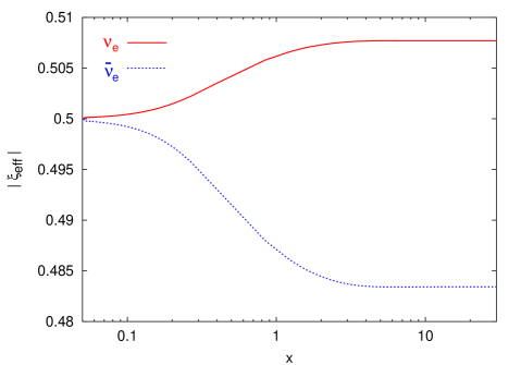
Figure 17: The evolution of the absolute value of the effective degeneracy parameter $\xi$ (if the distribution function is written in the equilibrium form) for electron neutrinos and antineutrinos with momentum $y=5$ ($\xi_{e}=0.5,\xi_{x}=1$).

The variations of temperature of the cosmic plasma in the case of strong degeneracy cannot be calculated on the basis of entropy conservation because entropy is not conserved if chemical potentials are non-vanishing. To this end one should use the covariant energy conservation law (18). The energy density of neutrinos with negative chemical potential is exponentially suppressed, $\rho\approx(3T^{4}/4\pi^{2})\exp(-|\xi|)$, and can be neglected. The total energy density of a certain neutrino flavor is given by

$$\rho_{tot}={T^{4}\over 8\pi^{2}}\left(\xi^{4}+2\pi^{2}\xi^{2}+{7\pi^{4}\over 15}\right)\approx{T^{4}\xi_{0}^{4}\over 8\pi^{2}R^{4}}\left[1-{4\pi^{2}\over 3\xi_{0}^{2}\left(R^{2}-1\right)}\right]\left(1+{2\pi^{2}R^{2}\over\xi_{0}^{2}}\right)$$ (208)

If we take into account only the leading, for large $\xi$, term in this expression then $\rho_{1}\sim 1/a^{4}$ and automatically satisfies the conservation law (18). In this case the remaining matter (photons, muons, electrons and positrons, etc) also satisfy this law and since their chemical potentials by assumption are vanishing, their entropy is conserved if they are decoupled from neutrinos, and the ratio $R=Ta/T_{0}a_{0}$ varies because of the annihilation of massive species. At the nucleosynthesis epoch it would be $R=(g_{*}^{0}/10.75)^{1/3}$. If $\nu\bar{\nu}$-annihilation is frozen at 100 MeV then $g_{*}^{(0)}=17.25$ and $R=1.17$; in the case of decoupling above QCD phase transition $g_{*}^{(0)}=47.75$ and $R=1.64$.

However the non-leading terms in $\rho_{1}$ that are of order of $1/\xi^{2}$ are quite essential and their presence destroys entropy conservation, so to find $R$ one has to solve numerically differential equation (18). The effect of these terms is to diminish $R$, so the results presented above can be considered the upper limits for $R$.

10.3 Degenerate neutrinos and primordial nucleosynthesis.

A possible role of neutrino degeneracy in big bang nucleosynthesis was noted already in the pioneering paper by Wagoner, Fowler, and Hoyle [426]. Even earlier the effects of neutrino degeneracy on $\beta$-reactions (58,59) were studied by Zeldovich [427] in old style cold universe model. After these works the effects of lepton degeneracy in BBN were analyzed in a number of papers [428]-[445], as well as in the quoted above ref. [425] (it is probably an incomplete list of references). The papers on this list differ chronologically by an increasing precision of essential physical parameters (in particular neutron life-time) and by increasingly accurate astronomical data. So in what follows we will quote only the results of the most recent works. The earlier papers are reviewed e.g. in ref. [114, 446, 91]

There are two physical effects from degenerate neutrinos that could influence primordial abundances. First, an increase of the energy density in comparison with non-degenerate case results in a faster expansion which in turn leads to a larger $n/p$-ratio at the onset of nucleosynthesis. Second, an asymmetry in the sector of electronic neutrinos/antineutrinos would strongly shift the equilibrium value of $n/p$-ratio, $n/p\sim\exp(-\xi_{\nu_{e}})$. That’s why the bounds on $\xi_{\nu_{e}}$ from BBN are much stronger than those for $\xi_{\nu_{\mu},\nu_{\tau}}$. The ratio of the extra energy densities of degenerate $\nu$ and $\bar{\nu}$ to the energy density of non-degenerate $\nu+\bar{\nu}$, under the assumption that $\xi=-\bar{\xi}$, is (see eq. (192)):

$$\Delta N_{\nu}={15\over 7}\left[\left({\xi\over\pi}\right)^{4}+2\left({\xi\over\pi}\right)^{2}\right]$$ (209)

If $\xi>2$ then one degenerate neutrino (plus antineutrino) species are equivalent to more than three ”normal” neutrinos and should be rejected. However, a positive (and rather small) chemical potential of $\nu_{e}$ would work in the opposite direction in BBN, so it is difficult to exclude a ”conspired” degeneracy of $\nu_{\mu,\tau}$ and $\nu_{e}$.

First we neglect a possible conspiracy and consider the effect of asymmetries of different neutrino families separately. It follows from the arguments presented above that chemical potentials of $\nu_{\mu,\tau}$ are bounded by the condition

$$\xi_{\mu,\tau}<1.5$$ (210)

if one extra neutrino species is permitted by the data on light element abundances (see sec. 6.1)

A possible role of electron asymmetry was studied in relatively recent works [442, 443]. The allowed range according to ref. [443] is $|\xi_{\nu_{e}}|<0.1$ with $4\leq\eta_{10}\leq 6$. A more sophisticated statistical analysis of ref. [442] gives somewhat different numbers $\xi_{\nu_{e}}=0.043\pm 0.040$ and $\eta_{10}=4.0^{+1.5}_{-0.9}$. However there are still some discrepancies in the data on light element abundances (in particular, high versus low deuterium controversy) and their interpretation, so possibly these numbers will be changed in future. One can expect a better accuracy in determination or restriction of the magnitude of neutrino degeneracy if the baryon number density is fixed by the CMBR data, independently from BBN.

A more interesting case is when all three chemical potentials are permitted to influence BBN. In that case the theory has two additional parameters in comparison with the standard model (the roles of $\xi_{\nu_{\mu}}$ and $\xi_{\nu_{\tau}}$ are the same because the essential quantity is the total energy density of $\nu_{\mu}$ and $\nu_{\tau}$) and the bounds on their values become much less restrictive. In particular, prior to measurements of the baryon density of the universe by CMBR, the freedom in the values of chemical potentials permitted the baryon-to-photon ratio to be much larger than in the standard BBN theory, allowing baryon dominated universe. Now it looks unlikely with any values of chemical potentials. Some decrease of $\eta$ with respect to the standard value is also possible, diminishing the conflict between visible and invisible baryons. The analysis made in refs. [440, 425] permits to conclude that $\eta$ can be as large as a hundred, so that even $\Omega_{B}=1$ is permitted. The appropriate values of chemical potentials are $\xi_{\nu_{e}}\sim 1$ and $\xi_{\nu_{\mu},\nu_{\tau}}\geq 10$. For that large values of $\xi_{\nu_{\mu},\nu_{\tau}}$ the freezing of reaction (194) takes place above 100 MeV and, according to eqs. (206,207), primordial values of $\xi_{\nu_{\mu},\nu_{\tau}}$ differ from those at BBN, while neutrino temperature at BBN remains equal to $T_{\gamma}$. If indeed $\xi>1$, then the energy density of degenerate neutrinos would be very large and the neutrinos could have an important impact on large scale structure formation. This problem and corresponding bounds on $|\xi|$ are discussed in the next subsection.

A combined analysis of the effect of simultaneous variation of all three chemical potentials on BBN was performed in the papers [439, 397, 92]. As is stressed in ref. [397], the authors carefully reexamined the decoupling temperature of neutrinos (see discussion in the previous subsection). They have found that the allowed range of variation of chemical potentials is

$$0\leq\xi_{\nu_{e}}\leq 1.4$$

$$0\leq|\xi_{\nu_{\mu},\nu_{\tau}}|\leq 40$$ (211)

for the baryonic density confined in the interval $0.1\leq\Omega_{b}h_{50}^{2}\leq 1$. These results are somewhat less restrictive than those found in ref. [92]. For low deuterium abundance the electronic chemical potential can roughly change in the interval $-0.25\leq\xi_{\nu_{e}}\leq 0.25$ for the total number of neutrino species changing from 1 to 16. The last number can be related to the muonic or tauonic asymmetry through the equation (200). The results are slightly different for high deuterium. The best fit values are $\xi_{\nu_{e}}=0.06$, $N_{\nu}=3.43$, and $\eta_{10}=5$ for low D and $\xi_{\nu_{e}}=0.35$, $N_{\nu}=13$, and $\eta_{10}=4.2$ for high D. Some inconsistency between the papers [397] and [92] is possibly related to a different evolution of the temperature of degenerate neutrinos. As is stated in ref. [92] the effect of non-standard value of neutrino temperature [141] is negligible. The latter is closer to the estimate of the evolution of neutrino temperature presented in the previous subsection. But the estimate is rather approximate and moreover, the spectrum of neutrinos may be noticeably distorted in the course of expansion because the elastic reaction rate is strongly energy dependent (204). A more accurate treatment of this problem is desirable.

The recent analysis [395], based on new measurements of the angular spectrum of CMBR, gives the limits:

$$-0.01<\xi_{\nu_{e}}<0.2,\,\,\,\,|\xi_{\nu_{\mu},\nu_{\tau}}|<2.6$$ (212)

under assumptions that the primordial fraction of deuterium is $D/H=(3.0\pm 0.4)\cdot 10^{-5}$ [109].

The results presented above are valid for homogeneous distribution of neutrinos. Possible inhomogeneities in lepton asymmetry at cosmologically large scale and strongly chemically inhomogeneous universe is discussed in sec. 7. Models of variation of lepton asymmetry in the sector of active neutrinos induced by the oscillations between active and sterile $\nu$’s are described in sec. 12.7. Small scale inhomogeneities in neutrino degeneracy and their impact on big bang nucleosynthesis are considered in ref. [447]. The scale of variation of leptonic chemical potentials are assumed to be sufficiently large, so the fluctuations in $\xi$ were not erased before BBN began (this corresponds to approximately 100 pc today). On the other hand, the scale is assumed to be smaller than the matter mixing scale so the resulting element distribution is homogeneous today. A surprising result is that in the case of the inhomogeneous scenario the total energy density of neutrinos is not bounded by BBN. Indeed one may have a regions with a very large and positive value of $\xi$ which gives a dominant contribution into the energy density but does not participate in the element formation, because for a very large $\xi$ the production of light elements is negligible. The model permits to enlarge considerably the upper limit on the baryon number density allowed by BBN, while the lower limit remains practically untouched: $3.0\cdot 10^{-10}<\eta<1.1\cdot 10^{-8}$ for $\xi_{\nu_{e}}\gg\xi_{\nu_{\mu},\nu_{\tau}}$ and $3.1\cdot 10^{-10}<\eta<1.0\cdot 10^{-9}$ for $\xi_{\nu_{e}}=\xi_{\nu_{\mu}}=\xi_{\nu_{\tau}}$. These upper limits correspond to $\Omega_{b}h^{2}=0.4$ and $\Omega_{b}h^{2}=0.036$ respectively.

In some papers a ”double” deviation from the standard scenario is considered - in addition to neutrino degeneracy another non-standard assumption is made. In ref. [444] inhomogeneous nucleosynthesis (induced by inhomogeneities in baryon distribution) with degenerate neutrinos is applied to the solution of a possible discrepancy between the observed low deuterium abundance in Lyman-$\alpha$ clouds and a possible overproduction of ${}^{4}He$. In ref. [445] primordial nucleosynthesis with varying gravitational constant and degenerate neutrinos is discussed.

Some more bounds on the neutrino degeneracy (energy density) follow from structure formation and cosmic microwave background, which are considered in the following subsections.

10.4 Degenerate neutrinos and large scale structure.

If degeneracy is large, the energy density of neutrinos would be much larger than that of non-degenerate ones and it would have a very strong impact on cosmological evolution. A trivial upper limit on the magnitude of degeneracy follows form the condition that neutrinos should not over-close the universe, $\Omega_{\nu}<1$. It gives

$$|\xi|=53h^{1/2}\Omega_{\nu}^{1/4}\left(2.73{\rm K}/T_{\gamma}\right)$$ (213)

To obtain this limit we used eqs. (20,43) and took neutrino temperature after $e^{+}e^{-}$-annihilation equal to $T_{\nu}=0.71T_{\gamma}$. It would be true if before the annihilation the temperatures were equal as is argued in subsection 10.2. This limit is stronger than those obtained in refs. [424, 425] where a smaller $T_{\nu}$ was used (see discussion in sec. 10.2), but still very weak. Even this rather weak limit excludes very high values of $\xi$ discussed in the previous section in connection with BBN.

A much stronger upper bound on $|\xi|$ is obtained from the condition that the universe must become matter dominated sufficiently early so that there would be enough time for large scale structure formation [424, 425]. (At RD-stage perturbations grow at most logarithmically and structure formation is ineffective [317].) Since at MD-stage perturbations rise as the scale factor $a(t)$ and the primordial density fluctuations are below $10^{-4}$, as is seen from temperature fluctuations of CMB, we assume that the equilibrium between matter and radiation should be earlier than red-shift $z=10^{4}$. It gives

$$|\xi|<5.3h^{1/2}\Omega_{m}^{1/4}\left(2.73{\rm K}/T_{\gamma}\right)$$ (214)

This limit is valid for massless neutrinos. Massive neutrinos have practically the same distribution as massless ones, i.e. the equilibrium one before decoupling and the rescaled distribution after decoupling:

$$f_{m}={1\over\exp\left(\sqrt{p^{2}(z_{d}+1)^{2}+m^{2}}\,/T_{d}-\xi\right)+1}\approx{1\over\exp(p/T_{\nu}-\xi)+1}$$ (215)

if their mass is much smaller than decoupling temperature, $T_{d}\sim{\rm MeV}$. Here $z_{d}+1=a(t)/a_{d}$ is the red-shift at decoupling and $T_{\nu}=T_{d}/(z_{d}+1)$. For $m_{\nu}\sim T_{d}$ nonequilibrium corrections to the spectrum are essential and the distribution may very much differ from the usually assumed rescaled one, see sec. 6.2 and ref. [150]. In this section we are interested in neutrinos with a small mass (in eV range or below) so for them we may use the distribution function (215). Such neutrinos become effectively non-relativistic when $m_{\nu}/T_{\nu}>0.2$; at that moment their pressure is about 0.1 of their energy density, while for relativistic gas $p/\rho=1/3$. Degenerate neutrinos have a larger average momentum and pressure, so they are more relativistic at the same $T/m_{\nu}$. Degenerate neutrinos become nonrelativistic at $m_{\nu}/T\sim\xi$ (if $\xi>10$) and the upper limit on their chemical potential, which follows from the condition that RD-stage was earlier than $z=10^{4}$, is $\xi<m_{\nu}/{\rm eV}$ (for a large $\xi$). On the other hand, neutrinos with masses larger than 10 eV and $\xi>2$ would over-close the universe because their number density is 5.3 times larger than the number density of non-degenerate neutrinos. So the bound (214) can be taken as a safe upper bound for both massive and massless neutrinos. Correlated bounds on neutrino mass and degeneracy based on their contribution into cosmological energy density were analyzed in refs. [448, 449]. It is indicated there that neutrinos may be cosmologically interesting even if they have a very small mass, $m_{\nu}<0.1$ eV, as follows from the data on neutrino oscillations. If the bound (214) is satisfied the contribution of such neutrinos into cosmological energy density could be as large as:

$$\Omega_{\nu}<0.037h^{-1/2}\Omega_{m}^{3/4}\,(m_{\nu}/0.1{\rm eV})$$ (216)

There are a few points however, where the results presented in ref. [448] disagree with our analysis. In particular, it is stated there that the decoupling temperature of degenerate neutrinos may be lower than that of non-degenerate ones, it may be even smaller that the electron mass. If this were the case, then the temperatures of relic neutrinos and photons at the present day would be equal. To come to this conclusion the authors of ref. [448] estimated the decoupling temperature from the usual condition of equality of expansion rate, $H$, and reaction rate, $\sigma n$, and substituted for $n$ the largest number density of participating particles, i.e. the number density of degenerate neutrinos. However, the reaction rate is given by $\dot{n}/n$ so the rate of elastic scattering of degenerate neutrinos on electrons, that maintain the equality of their temperatures, is proportional to electron number density as in the standard non-degenerate case (compare with the discussion in sec. 10.2). As a result, the authors of ref. [448] obtained a high value of $T_{\nu}$, while in other papers a much lower value found in ref. [425] was used. The estimates presented in the previous subsection give an intermediate result and some more work is necessary to confirm which value of $T_{\nu}$ is correct. Accordingly the limits on the values of $\xi$ presented here should be taken with caution.

The impact of massive degenerate neutrinos on structure formation was considered in refs. [424, 450, 449, 451, 397]. An extra free parameter, $\xi$ permits breaking rigorous connection between the neutrino mass, their energy density, neutrino free streaming and Jeans mass. A larger mass density of degenerate neutrinos permits having the same contribution of HDM into $\Omega$ with a smaller neutrino mass or permits a larger Hubble parameter for a fixed $m_{\nu}$. Degeneracy gives rise to somewhat larger free-streaming for a fixed $m_{\nu}$ and $h$ (because the average momentum of degenerate neutrinos is larger than that of non-degenerate ones). As shown in ref. [450] degenerate neutrinos may resolve inconsistency between mixed HCDM (hot+cold dark matter, $\Lambda=0$) model with observations, that appears if Hubble parameter is large, $h>0.5$.

An analysis of the power spectrum of density perturbations in a model with $\Omega_{\Lambda}=0.7$ was performed in ref. [449] both for massless and massive ($m_{\nu}=0.07$ eV) degenerate neutrinos. With an increasing $\xi$ the power at small scales is suppressed because a large degeneracy postpones the matter-radiation equality and correspondingly the fluctuations that enter horizon at RD-stage began to rise later. Another effect of neutrino degeneracy is a larger free streaming mentioned above. It leads to a further suppression of small scale matter fluctuations. In figure 18 taken from ref. [449] the region in the plane of neutrino chemical potential $\xi$ and spectral index of density perturbations $n$ is presented so that the model agrees with the observed large scale structure and CMBR, the latter is discussed in the next subsection.

Figure 18: LSS and CMB constraints in ($\xi$, $n$) space for $\Omega_{\Lambda}=0$ (left) and $\Omega_{\Lambda}=0.6$ (right). The underlying cosmological model is flat, with $h=0.65$, $\Omega_{b}=0.05$, $Q_{rms-ps}=18~{}\mu$K, no reionization, no tensor contribution. The allowed regions are those where the labels are. For LSS constraints, we can distinguish between degenerate neutrinos with $m_{\nu}=0$ (solid lines) and $m_{\nu}=0.07$ eV (dotted lines).

The idea to “save” the critical density universe with vanishing vacuum energy and $\Omega_{m}=1$, using freedom in neutrino degeneracy, was explored in ref. [452]. The authors concluded that the model with massless neutrinos failed to fit the observational data on large scale structure and CMBR anisotropies. If neutrinos have the mass of order 1 eV, a much better agreement with observations can be reached. However, with the latest results on the microwave anisotropy [71], the model encounters a serious problem with the observed baryon mass fraction in galactic clusters.

10.5 Neutrino degeneracy and CMBR.

The effects of neutrino degeneracy on the spectrum of angular fluctuations of CMB is discussed in recent papers [453, 454, 449, 451]. In the first one the analysis was done for massless neutrinos in $\Lambda=0$ cosmology, while in the other three the case of $\Omega_{\Lambda}=0.7$ was considered for massless [454] and for both massless and $m_{\nu}=0.07$ eV [449, 451] neutrinos. Another burst of activity [455, 396, 397, 92, 398] in this area was stimulated by the BOOMERanG [413] and MAXIMA-1 [414] measurements of CMBR anisotropies on sub-degree scales where a surprisingly small height of the second acoustic peak was observed. The new data [71], however, do not support this result. Still these papers are of interest because their arguments could be used to obtain the bounds on the neutrino degeneracy from CMBR.

The main effect of neutrino degeneracy, as we have already mentioned, is to delay matter-radiation equality, which results in a larger amplitude of the first acoustic peak and in a shift in the positions of the peaks toward higher $l$’s (see sec. 9). However the dependence on $\xi$ is not monotonic and for a large $\xi$ the hydrogen recombination may take place at RD-stage. This would give rise to a suppression of fluctuations and to a decrease of the peak height. According to ref. [449] this happens for $\xi>7$. The location of the first peak in this case would be at $l>450$, which disagrees with the data. Moreover such big $\xi$ contradicts the bound (214). Secondary peaks are influenced also by the damping at large $l$ and their amplitude could decrease with rising $\xi$. Another effect mentioned in these papers, a change of decoupling temperature for degenerate neutrinos [424, 425] and the corresponding decrease of $T_{\nu}$, possibly is not effective, as discussed in sec. 10.2. The results of the calculations of the angular spectrum of CMBR for different values of the degeneracy parameter $\xi$ are presented in fig. 19 taken from ref. [449].

Figure 19: Spectrum of angular fluctuations of CMB for different values of $\xi$ for one family of degenerate neutrinos; from bottom to top $\xi=0,3,5$. Massless and massive ($m_{\nu}=0.07$ eV) neutrinos are depicted by solid and dashed lines respectively. The appropriate cosmological parameters are chosen as $h=0.65$, $\Omega_{b}=0.05$, $\Omega_{\Lambda}=0.70$, $\Omega_{CDM}=1-\Omega_{b}-\Omega_{\nu}-\Omega_{\Lambda}$, $Q_{rms-ps}=18~{}\mu$K $n=1$. Reionization and tensor contribution are neglected. (from ref. [449])

One can see from this figure that neutrino degeneracy has a very strong impact on the height of the first peak. The height is almost twice larger for $\xi=5$ in comparison with $\xi=0$. One may conclude that $\xi>5$ does not fit the already existing data [454] if the data is interpreted in the frameworks of the standard cosmological model. On the other hand, a large neutrino degeneracy could help the survival of those cosmological models that predict a low first peak [449]. The future missions, MAP and Planck, could significantly improve the bounds on the neutrino degeneracy, roughly at the level $\delta\xi<0.1$, the accuracy strongly improving with rising $\xi$ [454]. On the other hand, in the case of considerable asymmetry, $\xi>3$, the future Planck mission will be able to measure neutrino mass at the level of 0.1 eV [451].

A small amplitude of the second acoustic peak observed in the earlier (preliminary?) data set [413, 414] in the frameworks of the standard model demanded a larger baryonic number density than was allowed by big bang nucleosynthesis [456, 457]. One possible way to diminish the height of the peak is neutrino degeneracy; it is discussed in the papers [455, 396, 397, 92, 398]. As we have seen in sec. 10.3, neutrino degeneracy permits having a much larger baryonic fraction than in the standard model. A larger value of $\Omega_{b}$ moves acoustic peaks to the right, and simultaneously enhances odd peaks against even ones. The small height of the second peak indicates a large baryon fraction. On the other hand, a larger fraction of relativistic matter, which can be achieved by a large chemical potential of $\nu_{\mu}$ or $\nu_{\tau}$, moves the peaks in the opposite direction and also increases the amplitude of the first peak, so the relative height of the second peak becomes smaller. In this sense it could mimic an increase of the baryon number. To ensure the necessary output of primordial abundances one can vary a small chemical potential of $\nu_{e}$. An unnatural feature of this scenario is an adjustment of two similar parameters $\xi_{\nu_{\mu},\nu_{\tau}}$ and $\xi_{\nu_{e}}$ in such a way that the first is large, while the second is small. Moreover, if there is mixing between $\nu_{e}$, $\nu_{\mu}$, and/or $\nu_{\tau}$ then for the LMA solution for solar neutrino anomaly all chemical potentials would acquire equal values (see sec. 12.6). On the other hand, for SMA solution an initially large $\xi_{\nu_{\mu},\nu_{\tau}}$ might naturally give rise through oscillations to a small $\xi_{\nu_{e}}$.

The values of chemical potentials and the baryon number density that are necessary to reach an agreement between the BBN and CMBR data are somewhat different in different papers but an agreement about gross features is manifest. According to the consistency plot between the number of effective neutrino species $N_{\nu}$ and the baryonic number density $\Omega_{b}h^{2}$ presented in the paper [398] agreement can be achieved approximately for $N_{\nu}=6-10$ and $\Omega_{b}h^{2}=0.025-0.030$, but with the latest data [71] the baryonic density shifts to $\Omega_{b}h^{2}=0.022\pm 0.004$.

11 Neutrinos, dark matter, and large scale structure of the universe.

11.1 Normal neutrinos.

Of all possible candidates for dark matter particles, neutrinos have a definite advantage: they are certainly known to exist and may naturally have a cosmologically interesting mass so that their contribution to $\Omega$ would be close to 1 (see sec. 4.1). All other candidates for the role of dark matter particles remain hypothetical. The suggestion that $\sim 10$ eV neutrinos could solve the problem of the missing mass of the universe was put forward in 1972 by Marx and Szalay [121] and by Cowsik and McClelland [458], see also [122]. The idea was elaborated in many subsequent publications [459]-[475] in the 1980s, especially by the Moscow group. Detailed investigations showed that neutrino-dominated universe would have large scale structure significantly different from the observed one and, though neutrinos may still remain one of essential components of dark matter, the dominant part most probably consists of new unknown particles (or fields). The situation was summarized in the late 1980s in ref. [476]. For more recent reviews on neutrino dark matter see e.g. refs. [477, 478, 479].

A strong argument against neutrino-dominated universe is that light neutrinos ($m=O({\rm eV}$)) permit formation of structures on a scale much larger then the galactic one, while the formation of galaxies is strongly inhibited and could take place rather late at red-shifts $z$ smaller or close to 1 [466, 470],[472]-[475]. The characteristic size of structures in neutrino-dominated universe can be estimated as follows. Neutrinos were decoupled from the cosmic plasma rather early, at $T\sim 2-3$ MeV, when neutrinos were relativistic. In the gas of non-interacting particles moving practically with the speed of light all perturbations with wave lengths smaller than the distances traveled by these particles until they become non-relativistic, are erased. Indeed, if in some region the number (and energy) density of neutrinos is larger than in nearby regions, the flux from neutrino-rich regions would be larger than the inverse flux from neutrino-poor regions and this evidently leads to equalization. The distance that neutrino passed, before it became non-relativistic, was roughly equal to $2t_{\nu}$, where $t_{\nu}$ was the time when the neutrino temperature dropped down to $T_{\nu}=m_{\nu}/3$. According to equations (45,47), $t_{\nu}=0.75m_{Pl}/m_{\nu}^{2}\approx 6\cdot 10^{12}\,{\rm sec}/(m_{\nu}/{\rm eV})^{2}$. Correspondingly, the mass contributed by neutrinos of one flavor inside the free-streaming radius is

$$M_{\nu}={4\pi(2t)^{3}\over 3}\rho_{\nu}=0.135\,m_{Pl}^{2}t_{\nu}=0.1\,{m_{Pl}^{3}/m_{\nu}^{2}}$$ (217)

where the numerical coefficient comes from the ratio of the energy density of one neutrino species to the total relativistic energy density: $\rho_{\nu}/\rho_{tot}=(1.36/3)/3.36=0.135$ with $\rho_{tot}=3m_{Pl}^{2}/32\pi t^{2}$. Thus we find that the smallest objects, which could be initially formed, have the mass [459, 461, 462]:

$$M_{\nu}\approx 1.5\cdot 10^{17}M_{\odot}\left(m_{\nu}/{\rm eV}\right)^{-2}$$ (218)

where $M_{\odot}=2\cdot 10^{33}$ g is the solar mass. In fact the mass is even larger because neutrinos did not stop when $T_{\nu}=m_{\nu}/3$.

The redshift when neutrinos became nonrelativistic is $z_{\nu}=1.4(m_{\nu}/3)/2.73\,{\rm K}=2\cdot 10^{3}(m_{\nu}/{\rm eV})$. Hence, the characteristic comoving size of the first formed structures is given by

$$l_{\nu}=2\,t_{\nu}(1+z_{\nu})\approx 250\,{\rm Mpc}\left({\rm eV}/m_{\nu}\right)$$ (219)

Neutrinos present an example of the so-called hot dark matter (HDM), which gives characteristic scale of the structures much larger than galactic size. The opposite case of dark matter giving $l\ll l_{gal}$ is called cold dark matter (CDM) and the intermediate one is naturally called warm dark matter (WDM).

Initially small density inhomogeneities started to rise when universe expansion became dominated by nonrelativistic matter. In the case of neutrinos, the change of regime takes place at the redshift given by the ratio of the present day energy densities of nonrelativistic matter represented by one massive neutrino species and relativistic matter containing cosmic microwave background radiation and two massless neutrino species:

$$z^{(eq)}_{\nu}=\left({\rho_{\nu}\over\rho_{rel}}\right)_{0}={112m_{\nu}/{\rm cm}^{3}\over 1.45\cdot 0.261\,{\rm eV/cm}^{3}}=3\cdot 10^{2}\left({m_{\nu}\over{\rm eV}}\right)$$ (220)

Thus the structures in the gas of cosmic neutrinos would be formed before hydrogen recombination ($z_{rec}\approx 10^{3}$) if $m_{\nu}>5$ eV. The result (220) would be trivially changed if there are several (2 or 3) massive neutrino species.

It was initially believed that structures smaller than $l_{\nu}$ (219) which are observed on the sky could be formed by fragmentation of the large sheets (Zeldovich pancakes) and filaments into galaxies. In other words, in universe dominated by neutrinos larger structures formed first and smaller ones appeared later (top-bottom scenario). However, as was argued in ref. [480], observations point to the opposite picture: our Galaxy seems to be considerably older than the Local Group. Moreover, numerical simulations [475] showed that universe dominated by light neutrinos is in disagreement with observations, or to quote the authors of ref. [475], “the conventional neutrino dominated picture appears to be ruled out”.

The idea that neutrinos might have a much shorter free-streaming length due to their self-interaction associated with the majoron exchange (see sec. 11.4), was proposed in ref. [481] and further discussed in ref. [482]. In such model, neutrinos indeed could behave similarly to cold dark matter at galactic scales. However they could not provide dark matter in dwarf galaxies (see the following paragraph).

Another strong blow to neutrino as the only form of dark matter was dealt by the Tremaine-Gunn limit [483]. The latter is a striking example of quantum phenomenon on cosmologically large scales. Neutrinos are fermions, so only one particle could be in a certain quantum state. Hence the total number of neutrinos in a galaxy cannot be arbitrarily large, and in order to constitute the total amount of galactic dark matter neutrinos must be sufficiently heavy. We assume that neutrinos form strongly degenerate gas with Fermi momentum $p_{F}=m_{\nu}V_{F}$, where $V_{F}$ is the neutrino velocity. The number density of galactic neutrinos (plus antineutrinos) is $n=2p_{F}^{3}/(6\pi^{2})$. Correspondingly the total mass of neutrinos in a galaxy with radius $R$ is equal to $N=4\pi R^{3}m_{\nu}n/3=(2/9\pi)(Rp_{F})^{3}m_{\nu}$. By virial theorem, velocity is related to gravitational potential $V^{2}_{F}=G_{N}M_{gal}/R$. This set of relations permit us to express $m_{\nu}$ through particle velocity around the galaxy and galactic radius:

$$m_{\nu}\approx 80\,{\rm eV}\left({300\,{\rm km/sec}\over V_{F}}\right)^{1/4}\left({1{\rm kpc}\over R}\right)^{1/2}$$ (221)

Thus, to provide all dark matter in small galaxies with $R\sim 1$ kpc and $V\leq 100$ km/sec neutrinos mush be heavier than $100$ eV, which goes against the Gerstein-Zeldovich limit (74,75).

The validity of Tremaine-Gunn limit was questioned by Ruffini and collaborators [484] who argued that numerical analysis does not support this limit. However it is difficult to see a flaw in the Tremaine-Gunn arguments presented above. Moreover, these arguments were applied in ref. [485] to a large number (1100) of galaxies with well measured rotational curves. It was shown that in order to be clustered on galactic scale neutrino mass should violate the Gerstein-Zeldovich limit.

The large free-streaming length and the Tremaine-Gunn limit have made the idea of purely neutrino dark matter rather unpopular and the attention has shifted to cold dark matter models. Particle physics proposes several possible candidates for CDM but none of them has been yet experimentally observed (see e.g. review [486]). After the magnitude of density fluctuations at large scales has been normalized by the COBE measurements [487], it has became clear that the simple CDM model with flat spectrum of primordial density fluctuations predicts too much power at small scales and requests some modifications. A possible resolution of the controversy was an assumption of a mixed CDM+HDM model [488]-[491] with about 30% of HDM and the rest in CDM. The mixed model revived the role of neutrinos as building blocks of the universe. The basic idea of why the model may work is easy to understand. At very large scales there is no difference between HDM and CDM. So the COBE data fixes their common contribution into density fluctuations. At smaller scales neutrino perturbations disappear and the remaining power becomes smaller than in the pure CDM model. Adjusting the new free parameter, the ratio $\Omega_{HDM}/\Omega_{CDM}$, one can achieve agreement between the size of density fluctuations at very large (horizon) scales and at galaxy cluster scales. Though both CDM and HDM dark matter look quite natural from the point of view of elementary particle physics, the similar magnitudes of their contributions into total cosmological energy density remains a mystery. This “cosmic conspiracy,” which includes also a similar contribution of baryons into $\Omega$ ($\Omega_{B}$ is at a per cent level) presents one of the most interesting challenges in cosmo-particle physics. A possible way to understand this conspiracy is discussed in a recent work [495]. Now we also have a contribution from vacuum or vacuum-like energy with $\Omega_{vac}\approx 0.7$, which strongly increases the gravity of the problem.

Despite this unexplained conspiracy (which is a common shortcoming of all models involving several types of dark matter), the mixed CDM+HDM model was quite popular for several years. With the fraction of mass density in HDM $\Omega_{HDM}\approx 0.3$ and the rest in CDM, $\Omega_{CDM}\approx 0.7$ (except for some small fraction in baryons), the model successfully described the observed gross features of large scale structures. In particular, the top-bottom scenario that was a shortcoming of pure HDM models, is reversed into a bottom-top one (i.e. smaller structures forming first) in the case of dominating cold dark matter. However it was noticed almost immediately after the mixed CDM+HDM model was proposed that the model had serious problems with the description of structures at high redshifts [496]-[498]. The problem originated from the fact that the hot component reduces the magnitude of perturbations at small scales, and if one uses the COBE normalization at large scales and assumes flat (Harrison-Zeldovich) spectrum of fluctuations, there would be too little power at small scales and galaxy formation would be delayed. This phenomenon is in disagreement with the observed abundances of damped Ly$\alpha$-systems at high red-shifts, $z\sim 3$, and quasars at $z\geq 4$. Numerical simulations of ref. [498] (see also [499]) in the frameworks of the reference model of that time with $h=0.5$, and baryonic fraction $\Omega_{B}=0.05$ lead to the conclusion that $\Omega_{\nu}<0.2$ and $m_{\nu}<4.7$ eV. The CDM+HDM model was defended in ref. [500], where it was argued that $\Omega_{\nu}=0.25$ is compatible with $z>3$ data. However, subsequent N-body and hydrodynamic simulations [501] indicate that a model with $\Omega_{\nu}\geq 0.2$ predicts an amount of gas in damped Ly$\alpha$-systems well below observations. Reducing $\Omega_{\nu}$ down to 0.2 (from the originally proposed 0.3) gives rise to an overproduction of clusters [502], because a smaller mass fraction of neutrinos results in a higher power at cluster scales. In a better shape is a model with several mass-degenerate neutrinos [502] with the same $\Omega$. It was suggested that $\nu_{\mu}$ and $\nu_{\tau}$ have almost equal masses close to 2.4 eV, so that the total $\Omega_{\nu}$ remains the same as in the model with a single massive neutrino with the mass 4.8 eV but the neutrinos became nonrelativistic later and have a larger free-streaming length. This leads to a lower abundance of clusters and to better agreement with data. However, good agreement was only reached for a rather low value of the Hubble parameter, $h=0.5$, while the observational data point toward a larger value, $h=0.65-0.7$. A recent discussion of hot dark matter with 2 or 3 degenerate neutrinos can be found in ref. [503]. A review of the state of art of HDM at the end of 20th century can be found in [504].

As we have already mentioned, the description of the large scale structure strongly depends upon the primordial spectrum of density fluctuations. Usually it is assumed that the spectrum is flat, i.e. perturbations of gravitational potential do not contain any dimensional parameters. This is the simplest possible spectrum and, moreover, it is predicted by the simplest inflationary models. Usually deviations from the flat spectrum are parameterized by a power law with the exponent $n$, see eq. (182). The flat spectrum corresponds to $n=1$. The assumption of $n=1$ was relaxed in refs. [405, 406], where the models of structure formation with massive hot neutrinos and $n>1$ were considered.

The form of the evolved spectrum depends upon the relative cosmological mass fraction of CDM and HDM. If HDM constituents are neutrinos, their number density in the standard model is fixed, $n_{\nu}=112/{\rm cm}^{3}$ (see sec 4.1) and thus $\Omega_{HDM}$ is determined by neutrino mass. The larger $m_{\nu}$ and $\Omega_{HDM}$ are, the stronger the suppression of density fluctuations at small scales is. This phenomenon is illustrated in fig 20 taken from reference [478].

Figure 20: Growth rate of the CDM density field, $f\equiv d\log\delta/d\log a$, in four flat C+HDM models at cosmological scale factor $a=1$ (solid) and 0.1 (dashed). The four models assume different neutrino masses: $m_{\nu}=1.2$, 2.3, 4.6, and 6.9 eV (from top down), corresponding to $\Omega_{\nu}=0.05$, 0.1, 0.2, and 0.3.

At large scales there is no difference between CDM and HDM, so that all the curves coincide. They start to deviate at smaller scales corresponding to neutrino free streaming length. The deviation becomes weaker with time because neutrino velocities drop in the process of expansion. One can see that a change in neutrino mass by 1 eV has a visible effect on the spectrum of density perturbations.

On the other hand, astronomical data accumulated over the past several years strongly indicates that cosmological constant is non-zero with $\Omega_{vac}\approx 0.7$ and $\Omega_{CDM}\approx 0.3$ (for discussion and a list of relevant references see e.g. the papers [505]-[510]). If this is indeed the case then there remains much less room for hot dark matter. Even if we assume that HDM makes 100% contribution into total density of matter, i.e. $\Omega_{HDM}=0.3$ and if we take the currently accepted value $h=0.7$, then from the limit (74) follows $\sum m_{\nu}<14$ eV. The data on neutrino oscillations (see sec. 2) show that the mass differences between different types of neutrinos are much smaller than 1 eV. If the oscillations take place between active neutrinos only, then they are nearly mass degenerate and their masses should be below roughly 5 eV. However, as we have already discussed, hot dark matter could not be dominant because in that case, short wave length perturbations would be efficiently erased and formation of small scale structures would be suppressed. This effect is stronger for a smaller $\Omega_{CDM}$. Hence in the models with non-zero cosmological constant and/or with a low $\Omega_{matter}$ the upper limit on neutrino mass is more restrictive.

The cosmological limits on the neutrino mass from the Ly$\alpha$ forest have been reanalyzed in ref. [511] for a larger range of values of the parameter $\Omega_{m}$ and with a recent Ly$\alpha$ forest measurements. The conclusion was that $m_{\nu}<5.5$ eV for all values of $\Omega_{m}$ and $m_{\nu}<2.4\,{\rm eV}\,\left(\Omega_{m}/0.17-1\right)$ for small $\Omega$, $0.2<\Omega<0.5$.

It was argued in ref. [512] that galaxy red-shift surveys could probe neutrino mass in eV range. The forthcoming data from the high precision Sloan Digital Sky Survey (SDSS) will permit to measure neutrino mass with an accuracy of

$$m_{\nu}\sim 0.65\,{\rm eV}\,\left(\Omega_{m}h^{2}/0.1N_{\nu}\right)^{0.8}$$ (222)

and even a mass as small as 0.01-0.1 eV is potentially observable in astronomy. Such strong result was obtained under the assumption that all other relevant cosmological parameters would be independently measured by CMB experiments at 1% level. To this end the standard theory of structure formation with adiabatic density perturbations and with linear scale independent bias have been used. The impact of 1 eV neutrinos on the galactic power spectrum is illustrated in fig. 21 taken from ref. [512] for high and low density of cosmic matter. The effect is very strong for $k\sim 0.1/{\rm Mpc}$, while the impact of such massive neutrinos on CMB spectrum is at the level of several per cent. It is worthwhile to redo these calculations for cosmology with non-zero Lambda.

Figure 21: Effect of a 1 eV neutrino on the bright red galaxy (BRG) power spectrum compared with expected precision of the SDSS BRG survey (1$\sigma$ error boxes). Upper curves: an $\Omega_{m}=1.0$, $h=0.5$, $\Omega_{b}h^{2}=0.0125$, $n=1$ model with and without a 1 eV neutrino mass. Lower curves: the same but for an $\Omega_{m}=0.2$, $h=0.65$ model.

As shown in ref. [513], the cluster abundance does not suffer from the biasing uncertainties and from the matching condition of the observed fluctuation power at COBE scale (several hundred Mpc) and at the cluster scale ($l_{cluster}=8h^{-1}$ Mpc). It permits to obtain the limit $m_{\nu}<0.6$ eV for the flat universe with $\Omega_{m}=0.3$ and $h<0.8$. For this matching, the Harrison-Zeldovich spectrum of fluctuations was assumed, $n=1$. If $n$ is significantly larger than 1, the limit becomes weaker. For the same set of cosmological parameters, and $n=1.2$ the limit is $m_{\nu}<1.4$ eV.

Another possible way of weighting neutrinos by astronomical means is to use gravitational lensing effects on background galaxies created by foreground large scale structures [514]. The physics behind this phenomenon is the same as discussed above, namely suppression of power at small scale by massive neutrinos and a reduction of the lensing signal. If all relevant cosmological parameters are measured with an accuracy of 10 per cent expected from the MAP mission, a weak lensing survey of 100 degrees squared could be sensitive to neutrino mass about 3.5 eV. For the survey of $\pi$ steradian down to 25th magnitude the limit could be 0.4 eV. With Planck satellite the limit could be further improved by factor 3-4. As is argued in the paper  [514], the advantage of this method is that it is free of bias and evolutionary effects.

An analysis of all available data on CMBR and large scale structures was performed in ref. [515]. As was already mentioned, the addition of hot dark matter reduces the power at small scales and to compensate this effect for e.g. $\Omega_{HDM}=0.05$ a blue tilt of primordial power spectrum, $n\approx 1.3$, is necessary. On the other hand, large $n$ gives too-large angular fluctuations of CMBR at small scales. They can be diminished by a significant tensor component or early reionization. For the flat spectrum of perturbations, i.e. $n=1$, and $h=0.65$ in $\Lambda CDM$ scenario of the structure formation, the upper bound on the amount of hot dark matter is $\Omega_{\nu}<0.05$ or $m_{\nu}<2$ eV. With a possibility that $n$ can vary the limit is twice weaker.

A detailed study of all cosmological parameters, based on the large scale structure observations at different scales and angular fluctuations of CMBR together with the BBN data and measurements of the Hubble constant, was performed in a series of papers [516, 517, 518]. The best fit model is $\Lambda$-dominated, with $\Omega_{\Lambda}\approx 0.7$ and with 8% contribution of neutrinos into clustered dark matter, or $\Omega_{\nu}=0.03^{+0.07}_{-0.03}$. The upper limit on the neutrino mass is $m_{\nu}<4$ eV. A more recent analysis of ref. [519] lead to the conclusion that $\Omega_{\nu}=(0-0.2)\,\Omega_{matter}$.

To summarize, the study of details of large scale structure permits obtaining an upper limit on neutrino mass that would be considerably stronger than the Gerstein-Zeldovich limit, which is based solely on considerations of the total cosmological energy density. However, the latter is model-independent while the former demands very accurate measurements of basic cosmological parameters. Moreover, some essential assumptions about the structure formation should be made. In particular, the simplest form of the spectrum of primordial fluctuations, Gaussian statistic of the fluctuations, and their adiabatic character are assumed. In principle all these assumptions can be tested by other astronomical observations, especially by precise measurements of angular spectrum of CMB with the Planck mission accuracy. Still the problem of degeneracy persists and it is a difficult task to separate the effects of different parameters. On the other hand, the best direct limit that can be expected from the total cosmological density could be hardly stronger than 10 eV, while the bounds discussed above may be much better.

11.2 Lepton asymmetry and large scale structure.

The results of the previous subsection were obtained under the standard assumption that the lepton asymmetry in neutrino sector is negligibly small. Strictly speaking this is not known and the data permit rather large chemical potentials of $\nu_{\mu}$ and $\nu_{\tau}$, see sec. 10.3, $\xi=\mu/T\geq 1$. An extra parameter, $\xi$ permits to break the rigid relation between neutrino mass and their cosmological energy density:

$$\rho_{\nu}(\xi)=\rho_{\nu}(0)\left[1+{\xi^{3}\over 9\zeta(3)}+{\pi^{2}\xi\over 9\zeta(3)}-{2\left(1-e^{-\xi}\right)\over 3\zeta(3)}\int_{0}^{\infty}{dy\,y^{2}\over\left(e^{y}+1\right)\left(e^{y+\xi}+1\right)}\right]$$ (223)

where $\zeta(3)\approx 1.202$ and the dimensionless chemical potential $\xi$ is positive. Note that this expression is different from eq. (192), because the latter is valid for relativistic neutrinos, while the former is true for non-relativistic neutrinos - it is simply $\rho=mn$, where $n$ is the number density. The energy density $\rho_{\nu}(\xi)$ is an increasing function of $\xi$, so for a degenerate neutrino gas the same energy density could be achieved with smaller $m_{\nu}$. Another difference from the standard model is that the average momentum of degenerate neutrinos is somewhat higher than that of non-degenerate ones with the same mass, so degenerate neutrinos are more relativistic. Correspondingly their free streaming path is larger.

A mixed dark matter model with non-vanishing chemical potentials of neutrinos was considered in ref. [450]. The introduction of the additional parameter, $\xi$, helps alleviate some problems of (H+C)DM models discussed in the previous subsection. A larger $\Omega_{\nu}$ with the same $m_{\nu}$ permits higher values of the Hubble parameter, $h>0.5$, while a bigger free-streaming length diminishes the destructive influence of neutrinos on the damped Ly$\alpha$-system. For more detail see sec. 10.4.

Structure formation with degenerate neutrinos was considered in the papers [453, 449]. In the first one it was shown that a model with massless neutrinos with chemical potential $\mu_{\nu}=3.4T$ together with the usual cold dark matter gives a good description of the large scale structure in $\Lambda=0$ universe and of the anisotropy of CMBR (see sec. 10.5). In the subsequent paper [449] the scenario was generalized both to massless and massive neutrinos and cosmology with non-zero Lambda-term.

11.3 Sterile neutrinos.

A much richer zoo of possible forms of dark matter becomes open if one permits the existence of sterile neutrinos, $\nu_{s}$, which interact much weaker than the usual, active, ones, or if one allows usual neutrinos to have stronger, than normal weak, interaction (for the latter see the next subsection). A recent review on physics of sterile neutrinos can be found in [520]. The simplest way to produce sterile neutrinos is to assume that neutrinos have both Majorana and Dirac masses. The simultaneous existence of both types of mass excites right-handed (sterile) neutrino states which are produced from the active ones by oscillations [54]. If equilibration with respect to sterile states was not achieved, then their number density could be smaller than the number density of active neutrinos and correspondingly the Majorana mass of $\nu_{s}$ could be around keV without violation of the Gerstein-Zeldovich limit. However, sterile right-handed neutrino states, $\nu_{R}$, are not necessarily created through oscillations. They could be thermally produced at an earlier hot stage in equilibrium abundance, and cosmology allows their mass to be larger than the mass of their left-handed companions because the number density of right-handed states is suppressed by the entropy factor (see section 6.4 where production of right-handed neutrinos is discussed). This mechanism for making warm dark matter from $\nu_{R}$ was considered in ref. [521].

Another way to create warm dark matter from neutrinos was proposed in ref. [130], where the cosmological scenario with a very low reheating temperature was considered. In this model the cosmological number density of normal active neutrinos could be much smaller than the usual 100 $/cm^{3}$ and their mass is not subject to Gerstein-Zeldovich limit, sec. 4.1. A model with 4 neutrino mixing, based on this scenario of low temperature reheating, was considered in ref. [522]. It was assumed that $\nu_{\mu}$ or $\nu_{\tau}$ with keV mass form warm dark matter, while solar neutrino anomaly is explained by the mixing between $\nu_{e}$ and a light sterile neutrino. However, the new SNO data [36] disfavors the $\nu_{e}-\nu_{s}$ solution of the solar neutrino problem, and though some (even large) mixing of active and sterile neutrinos is not excluded, the concrete values of the parameters used in the paper [522] are not realistic.

The idea of “using” sterile neutrinos as warm dark particles was further pursued in ref. [523] with production of $\nu_{S}$ through oscillations. WDM cosmology is considered in more detail in subsequent research [524]. Present day data indicate that warm dark matter together with cold dark matter may resolve some problems with galaxy properties that exist in CDM scenario (for discussion, literature, and possible candidates for WDM see e.g. ref. [525]). Thus, WDM may become a respectable member of dark member community [526]. Recently the properties of warm dark matter particles were strongly constrained by Lyman-alpha forest [527] and by cosmological reionization [528]. The lower limits on their mass are respectively 0.75 keV and 0.5 keV.

A dark matter model with sterile neutrinos but with an unusual, non-thermal, spectrum was considered in paper [529]. It was noticed some time before [530] that neutrino oscillations can strongly distort the spectrum of active neutrinos and also create sterile neutrinos with a non-thermal spectrum. As was shown in ref. [529], $\nu_{s}$ could be produced by neutrino oscillations in the early universe, but in contrast to the previous case, in the presence of a rather large cosmological lepton asymmetry, about 0.001-0.1. In this case the production proceeds mostly through resonance conversion, and the resonance condition is fulfilled only for low energy $\nu_{s}$ (see section 12.5). Thus, non-relativistic $\nu_{s}$ are predominantly produced even though they are very light, with the mass in the interval of 0.1-10 keV. Because of the cold non-thermal spectrum of $\nu_{s}$ they move more slowly than the usual warm dark matter particles, so the authors of ref. [529] propose to call such dark matter “cool”. In this model the cut-off in the spectrum of density perturbations could be around the dwarf galaxy scale or even below.

A new heavy neutral fermion with several GeV mass was proposed in ref. [531], in a particular model with an extended Higgs sector, as an explanation of the gamma-ray emission from the galactic halo. This is completely analogous to the annihilation of heavy leptons described in sec. 5.1. The energy density of such fermions could be cosmologically interesting and they might contribute noticeably to cold dark matter. However, these particles are not mixed with active neutrinos and calling them ”neutrinos” is rather arbitrary.

Naturally light sterile neutrinos appear in a large class of supersymmetric models with gauge mediated symmetry breaking [532]. These neutrinos have mixing with the active ones at the level of $10^{-4}$ and mass in the interval of 10 eV - 1 keV. Their number density, created by oscillations in the early universe, may be sufficiently high to make them cosmologically interesting and to provide a warm component to dark matter.

Sterile neutrinos may appear in our universe from mirror or shadow worlds (see sec. 14). Their implications for structure formation are essentially the same as of “normal” sterile neutrinos. Depending upon the mass difference between active and sterile $\nu$’s the latter could constitute hot, warm, or even cold dark matter. On the other hand, judging by the existing indications to neutrino oscillations, the mass differences between different neutrino species are small, though some heavy $\nu_{s}$ are not excluded.

The production of $\nu_{s}$ through oscillations could result in a smaller number density of active neutrinos because the total number of active plus sterile neutrinos was approximately conserved at later stages, when the active neutrinos decoupled from the plasma. The energy density of mirror/shadow particles must be smaller than that of the usual ones, otherwise there would be serious problems with nucleosynthesis, or a charge asymmetry in $\nu_{e}-\bar{\nu}_{e}$ sector must exist to compensate the effect of larger energy density of relativistic species at BBN. In ref. [533] an exact parity model (exact mirror symmetry) was considered with a heavier $\nu_{\tau}$ and light mirror neutrinos. The number density of $\nu_{\tau}$, which constitute hot dark matter particles in this model, could be smaller than the standard one because of the above mentioned effect of conversion of $\nu_{\tau}$ into mirror neutrinos. With the parameters taken in that paper the authors obtained $n_{\nu_{\tau}}=0.7n_{\nu}^{standard}$. This means that effective number of neutrino generations participating in dark matter becomes non-integer and allows for a larger mass of HDM neutrinos. The particular example considered in [533] was $5\,\,{\rm eV}<m_{\nu_{\tau}}<10\,\,{\rm eV}$. Another possible effect related to the existence of sterile (mirror) neutrinos that could be important for structure formation is that the energy density of relativistic particles at the moment when heavier neutrinos became non-relativistic could be different from that of the standard model [533]. Thus, the model with sterile neutrinos allows more freedom in comparison with the standard hot dark matter model and may better agree with the data.

In the case of broken mirror parity [534] it is natural to expect sterile neutrinos with a mass in the keV range and with a cosmological abundance of roughly two orders of magnitude below the standard neutrino abundance (73). Such neutrinos are also good candidates for warm dark matter particles [535, 536].

Usually the production of sterile neutrinos in the cosmological plasma proceeds through their mixing with active ones, so the equations derived in secs. 12.4, 12.5, 12.8 for the mixing with light sterile $\nu$ are directly applicable here. The calculations of the production of heavy sterile (WDM) neutrinos through mixing with active ones were performed in the paper [523]. The calculations were based on equation (445) but in contrast to the previous works the production rate of active neutrinos was not averaged over neutrino spectrum but taken with an explicit energy dependence. It permits calculating the spectrum of the produced $\nu_{s}$. The latter was found to be the same as the spectrum of active neutrinos mixed with $\nu_{s}$ [523, 537]. In the second paper the factor 2 was corrected, as shown in sec. 12.4, eq. (333). Hence the cosmological number density found in ref. [537] is twice smaller than that found in ref. [523].

The relative number densities of sterile neutrinos mixed with an active flavor $\nu_{a}$, $r_{s}^{a}=n_{s}/n_{eq}$, according to the results of the paper [537] are

$$r_{s}^{e} = 1.8\cdot 10^{5}\sin^{2}2\theta\left(m/{\rm keV}\right)(10.75/g_{*}(T_{prod})^{3/2}\,,$$ (224)

$$r_{s}^{\mu,\tau} = 2.5\cdot 10^{5}\sin^{2}2\theta\left(m/{\rm keV}\right)(10.75/g_{*}(T_{prod})^{3/2}$$ (225)

where the correction factor $(10.75/g_{*}(T_{prod})^{3/2}$, due to entropy generation, is included. Here $T_{prod}$ is the effective temperature of production of sterile neutrinos given by $T_{s}\approx 100\,{\rm MeV}\,(m/{\rm keV})^{1/3}$ (see discussion in sec. 12.4, eq. (351)).

If sterile neutrinos indeed constitute the dark matter, then their number density can be found from $\rho_{s}=10\,\Omega_{DM}\,h^{2}\,$keV/cm³, which gives

$$r_{s}\equiv{n_{s}\over n_{a}}=1.2\cdot 10^{-2}\,\left(\frac{\mbox{keV}}{m}\right)\left(\frac{\Omega_{DM}}{0.3}\right)\left(\frac{h}{0.65}\right)^{2}\,.$$ (226)

Thus, comparing eqs. (224, 225) with eq. (226) we find the necessary values of mass/mixing:

$$\sin^{2}2\theta_{se}\approx 6.7\cdot 10^{-8}\left({{\rm keV}\over m}\right)^{2}\left({g_{*}(T_{prod})\over 10.75}\right)^{3/2}\left(\frac{\Omega_{DM}}{0.3}\right)\left(\frac{h}{0.65}\right)^{2},$$ (227)

$$\sin^{2}2\theta_{s\mu}\approx 4.8\cdot 10^{-8}\left({{\rm keV}\over m}\right)^{2}\left({g_{*}(T_{prod})\over 10.75}\right)^{3/2}\left(\frac{\Omega_{DM}}{0.3}\right)\left(\frac{h}{0.65}\right)^{2},$$ (228)

The mass eigenstate, the heavier neutrino, $\nu_{2}$, does not completely coincide with $\nu_{s}$. It has an admixture of an active $\nu$, proportional to $\sin\theta$. Because of this mixing $\nu_{2}$ is coupled to the intermediate $Z^{0}$-boson and it allows for the decay:

$$\nu_{2}\rightarrow\nu_{1}+\ell+\bar{\ell}\,,$$ (229)

where $\nu_{1}$ is mostly an active flavor and $\ell$ is any lepton with a mass of less than half the mass of the heavy neutrino. Following ref. [537] we express the decay life-time as:

$$\tau=\frac{10^{5}\,f(m)}{m(\mbox{MeV})^{5}\,\mbox{sin}^{2}2\theta}\,\,\mbox{sec}\,,$$ (230)

where $f(m)$ takes into account the open decay channels (for $m<1$ MeV only the neutrino channels are open, and $f(m)=0.86$, while for $m_{s}>2m_{e}$ the $e^{+}e^{-}$-channel is also open and $f=1$). Now, for the sterile neutrino to be a dark matter particle we must demand that it does not decay on cosmic time scales, which means $\tau>4\times 10^{17}$ sec, and hence from eq. (230) we get

$$\mbox{sin}^{2}2\theta<2.5\times 10^{-13}\,\frac{f(m)}{m(\mbox{MeV})^{5}}\,.$$ (231)

We can obtain a stronger bound considering the radiative decay

$$\nu_{s}\rightarrow\nu_{a}+\gamma\,,$$ (232)

where $\nu_{a}$ is any of the active neutrinos. This decay will contribute with a distinct line into the diffuse photon background near $m/2$. The branching ratio for the reaction (232) was found [287] to be: $BR\approx 1/128$. The flux of electromagnetic radiation form the decay was calculated in the papers [342, 343] (see also refs. [62, 538]). In the case of a life-time larger than the universe age, and of the matter dominated flat universe the intensity of the radiation in the frequency interval $d\omega$ is equal to:

$$dI=(BR)\,{n_{s}^{(0)}\over H\tau_{s}}\,{\omega^{1/2}d\omega\over(m_{s}/2)^{3/2}}$$ (233)

where $n_{s}^{(0)}$ is the present-day number density of $\nu_{s}$ and $H$ is the Hubble constant (compare to eq. (177) of sec. 8.4). We neglected here some corrections related to a possible dominance of the lambda-term in the latest history of the universe.

In the relevant energy range a rather conservative upper limit on the flux of electromagnetic radiation is (see e.g. ref. [313]):

$$\frac{d{\cal F}}{d\Omega}<0.1\,\left(\frac{1{\rm MeV}}{E}\right){\rm cm}^{-2}{\rm sr}^{-1}{\rm sec}^{-1}$$ (234)

Thus taking the accepted now values $\Omega_{s}=0.3$ and $h=0.65$ we find: $\tau>4\times 10^{22}$, which leads to the bound

$$\mbox{sin}^{2}2\theta<2.5\times 10^{-18}\,\frac{f(m)}{m(\mbox{MeV})^{5}}\,.$$ (235)

The mass-mixing relation for warm dark matter consisting of sterile neutrinos is presented in fig. 22 taken from ref. [537].

Figure 22: Bounds for $(\nu_{\alpha}-\nu_{s})$-mixing. The middle full line describes the mass-mixing relationship if sterile neutrinos are the dark matter for $(\nu_{\tau}-\nu_{s})$-mixing. The two other full lines allow a factor 2 uncertainty in the amount of dark matter, $\Omega_{DM}=0.15-0.6$. The dashed line is for $(\nu_{e}-\nu_{s})$-mixing. The hatched region for big masses is excluded by the Diffuse Gamma Background. The region above the dotted line is excluded by the duration of SN 1987A for $(\nu_{\tau}-\nu_{s})$-mixing. (for discussion and references see the paper [537])

Recently there appeared a paper [539] where the problems of production of sterile neutrinos and their role as possible warm dark matter were addressed both for resonance and non-resonance cases. The number density of sterile neutrinos obtained in that paper for non-resonance case is

$$\Omega_{\nu}h^{2}=0.3\,(\sin 2\theta/10^{-5})^{2}\,(m/100{\mbox{keV}})^{2}.$$ (236)

It is about $(7-10)$ times smaller than the results (224,225) for $g_{*}(T_{prod})=10.75$ and differs by twice larger factor , i.e. by $(14-20)$ from reference [523]. One could attribute the disagreement to different treatment of of the cooling rate $T(t)$, entropy production, etc. In view of the potential importance of sterile neutrinos as warm dark matter particles, it is desirable to make an additional study to resolve this discrepancy.

In a subsequent paper [540] direct detection of sterile neutrino warm dark matter by the observation of the X-ray line with the energy below 2.5 keV was suggested. The authors obtained the upper limit $m_{\nu_{s}}<5$ keV using the result (236) of ref. [539] for $\nu_{s}$ mass density and the existing data on the X-ray background. However, the limit is substantially weakened if $\nu_{s}$ are produced resonantly due to a large primordial lepton asymmetry [529]. The range of photon energies, where the line from the decay of $\nu_{s}$ can be observed, was narrowed in ref. [541]. It was argued there that the lower limits on $m_{\nu_{s}}$ [527, 528] should be strengthen by factor 3.4 for the particular case of $\nu_{s}$ produced with a smaller temperature, and correspondingly softer spectrum than normal neutrinos. This argument together with the result of ref. [540] constraints the mass of $\nu_{s}$ in the range 2.6 - 5 keV and the X-ray line, to be looked for, between 1.3 and 2.5 keV.

11.4 Anomalous neutrino interactions and dark matter; unstable neutrinos.

As we have already mentioned, the cosmological upper limit on neutrino mass (74) would not be applicable if the number density of neutrinos becomes smaller than the standard value (73). There are several possible ways to achieve that. Neutrinos could be very weakly coupled to ordinary matter, so they were never abundantly produced. In the case of sterile neutrinos considered above, the production proceeds through oscillations and they never abundantly produced. Another possibility is an early decoupling of sterile neutrinos, and though they were in thermal equilibrium at high temperatures, their present-day abundance is diluted by the entropy release i.e. by the ratio of the number of particles species in the plasma at the moment of decoupling of active $\nu$ to that at decoupling of sterile $\nu$, $g_{*}^{(fin)}/g_{*}^{(in)}$. Since $g_{*}^{(fin)}=10.75$, one needs the decoupling of $\nu_{s}$ to take place at electroweak scale or above to ensure suppression by an order of magnitude.

Another possible way to diminish the number density of cosmic neutrinos is to assume that they, on the contrary, have an additional, stronger than weak, interaction. In that case neutrinos would remain longer in thermal equilibrium and at the moment of freeze-out their number density would be suppressed by the Boltzmann factor, $\exp(-m_{\nu}/T)$. For this mechanism to be operative, the interactions should be strong enough and the neutrino mass, $m_{\nu}$, should be sufficiently high. Such a possibility is naturally realized, for example, in the models of spontaneous breaking of leptonic charge conservation [56, 127, 236] or breaking of family symmetry [57]. As we have already mentioned, in this case, due to the Goldstone theorem, there appears a new light (or massless) (pseudo)goldstone boson-majoron, $J$, (or familon) with the Yukawa coupling to neutrinos:

$${\cal L}_{\nu,J}=g_{ik}\,J\,\bar{\nu}_{i}\gamma_{5}\nu_{k}+...$$ (237)

where $g_{ik}$ are the coupling constants of majoron to neutrino species $i$ and $k$ and multi-dot stands for higher order terms in the coupling constant. This interaction not only could reduce the cosmological number density of massive neutrinos but also induce the decay of heavier neutrino $\nu_{h}$ to a lighter one and majoron, if $m_{J}<m_{\nu_{h}}$ (see sec. 6.3,8).

The idea that cosmological number density of neutrinos could be strongly depleted through annihilation into light or massless bosons was proposed and elaborated long ago [542]-[545]. Depending on the parameters of the model and, in particular, on the value of $m_{\nu}$, massive stable neutrinos could dominate cosmological energy density and constitute either cold or warm dark matter. If light scalar bosons do not exist, then one may diminish cosmological number density of massive neutrinos assuming that the latter have a large magnetic moment [263], $\mu_{\nu}\sim 10^{-6}$ Bohr magneton. However this value contradicts the limits on the neutrino magnetic moment discussed in sec. 6.5 as well as the experimental measurements (13). Thus, as it was concluded in ref. [546], tau-neutrino with MeV mass cannot constitute cosmological dark matter.

The majoron model naturally opens two interesting possibilities for neutrino dark matter:
1) a stable $\nu$’s providing warm or even cold dark matter; neutrinos could be either rather heavy with a smaller than normal cosmological number density or have a strong self-interactions reducing their mean-free path, as mentioned in subsection 11.1 [481, 482];
2) an unstable dark matter either with a heavy $\nu$ decaying into majoron and light $\nu$ or with majoron decaying into a pair of neutrinos.
The role that unstable neutrinos might play in the large scale structure formation was briefly mentioned in ref. [159], where the bound on their life-time was derived from the condition that the universe could not be radiation dominated during the epoch of galaxy formation (see sec. 8.2). A more constructive idea to describe the observed structure of the universe with pure neutrino dark matter, using heavy unstable neutrinos and lighter stable ones was proposed a little later in the paper [547]. The authors argued that neutrinos with masses about 100 keV would preserve and amplify initial perturbations on galactic scales. Their life-time should be small in comparison with the universe age to avoid the Gerstein-Zeldovich bound. On the other hand the life-time should be long enough so that the perturbations would not be washed out after heavy neutrino decay. For further amplification of perturbations the heavy neutrinos should decay a little after light neutrinos (with $m_{\nu}\sim 100$ eV) became nonrelativistic. An alternative possibility of preserving galactic scale perturbations until light neutrinos became nonrelativistic is to introduce large amplitude fluctuations at small wave length, such as primordial black holes with masses $10^{9}M_{\odot}$ [547].

Detailed works of the 1980s with the same idea to save pure neutrino dark matter with heavier unstable $\nu$’s can be found in refs. [548]-[554]. More general scenarios of decaying particle cosmology, when the particles in question are not necessary neutrinos, are considered in the papers [555, 316]. In ref. [549] only the decays of heavy neutrino into known particles were permitted: $\nu_{h}\rightarrow\nu_{l}\,\gamma$, $\nu\rightarrow e^{+}\,e^{-}\,\nu_{l}$, or $\nu_{h}\rightarrow 3\nu_{l}$. Radiative decays are very strongly restricted now, see secs. 8.3,8.4,11.3 and fig. 22 and permit the exclusion of a large range of parameter values, while the decay into invisible $3\nu$ channel might be a viable option. The life-time with respect to this decay is given by eq. (230). With $m_{\nu}<2m_{e}$, so that the decay into $e^{+}e^{-}\nu$ is forbidden, this life-time could be cosmologically permitted and interesting for the structure formation.

There is considerably more freedom in the decaying particle model of structure formation if new decay channels are allowed, in particular, decays into lighter $\nu$ and a (pseudo)goldstone boson majoron or familon. This idea was proposed almost simultaneously in several papers [548, 550, 551]. A more complicated model with several decaying particles (heavy neutrinos), and cold (axion) and hot (light neutrinos) dark matter is considered in ref. [556].

A new burst of interest to the structure formation with decaying particles arose in the middle of 90th after COBE [487] fixed the normalization of the power spectrum of density fluctuations at large scales. If one assumes that the universe is dominated by cold dark matter and that the spectrum of fluctuations is flat, then one can use the COBE normalization to calculate the power at galactic and cluster scales. The results were about twice larger than the astronomical measurements. This meant that the simple one-component dark matter scenario was ruled out and some modifications of the latter need to be found. Several papers appeared almost simultaneously that considered the decaying neutrino model of structure formation. Essentially two distinct possibilities were explored: tau-neutrino with an arbitrary mass from a fraction of keV up to several MeV [222, 223],[558]-[565] and, somewhat earlier, a new 17 keV neutrino [566, 567, 218, 568], now dead. The paper [566] is essentially based on ref. [569] where the case of a neutrino with a mass in keV range and a life-time of about $10^{4}$ years was considered. It is shown that such neutrinos would provide the necessary extra power on galactic scale. A detailed analysis of perturbation growth in the universe with unstable neutrinos having the mass and life-time in the intervals $30\,{\rm eV}<m_{\nu}<10\,{\rm keV}$ and $10^{7}\,{\rm sec}<\tau_{\nu}<10^{16}\,{\rm sec}$ respectively, was performed in ref. [570].

A new idea was proposed in ref. [218], namely that the bosons, $B$, from the decay of relativistic 17 keV neutrinos through the channel $\nu_{17}\rightarrow\nu+B$ could form a Bose condensate producing cosmologically interesting cold dark matter. The model was further developed and corrected in refs. [571]-[574] for an arbitrary type of decaying neutrino. The energy spectrum of the bosons produced in the decay could be quite different from the thermal one. A large part of them is produced at small momenta, while some are still relativistic. The scenario permits to obtain simultaneously two forms of dark matter: cold and hot ones with comparable contributions into $\Omega$. However in the simplest version of the scenario only 35% of matter is cold and about 60% is hot. The fraction of CDM could be somewhat enhanced if a sequence of the decays: $\nu_{\tau}\rightarrow\nu_{\mu}+B$, $\nu_{\tau}\rightarrow\nu_{e}+B$, and $\nu_{\mu}\rightarrow\nu_{e}+B$ was effective.

The scenarios with decaying particles have some common basic features that are illustrated below on the examples of models presented in several different papers. There are two main effects important for structure formation: an increase of a fraction of relativistic matter by the products of the decay and a possible earlier MD stage prior to the decay of a heavy original particle.

In the scenario of ref. [223] a tau-neutrino with a mass in the interval of 1-10 MeV and a rather short life-time 0.1-100 sec was considered. The role of such neutrino in primordial nucleosynthesis is discussed in sec. 6.3. Its impact on structure formation proceeds through an increase of energy density in relativistic particles produced by the decay of $\nu_{\tau}$. An excess of relativistic energy would shift the moment of equality between matter and radiation to a later time and would modify the spectrum of evolved perturbations. Indeed, perturbations with the wave length $\lambda$ larger than horizon evolve in the same manner, so that their spectrum is preserved. If a certain wave enters horizon at MD stage, the perturbation continue rising as they did before, so the transfer function relating primordial perturbations to the evolved ones may be taken as being equal to unity, $f_{tr}(\lambda)=1$ However, if perturbation enters horizon earlier at RD stage, the amplitude of such perturbation essentially freezes so its relative magnitude becomes smaller. It can be checked that the transfer function can be taken as

$$f_{tr}(\lambda)=(\lambda/\lambda_{eq})^{2},\,\,\,{\rm for}\,\,\,\lambda>\lambda_{eq}$$ (238)

where $\lambda_{eq}$ is the wave length that entered horizon at a time when the energy densities of nonrelativistic and relativistic matters were equal. According to ref. [223]:

$$\lambda_{eq}\approx 10\,{\rm Mpc}\,\left(\Omega h^{2}\right)^{-1}\left(g_{*}/3.36\right)^{1/2}$$ (239)

One can see from these arguments that an increase of $\lambda_{eq}$ would diminish the power at scales $\lambda<\lambda_{eq}$ and would help resolve the discrepancy between COBE and cluster scales.

Another effect associated with unstable particles is that prior to their decay they might dominate the cosmological energy density, so the universe would be in an early temporary MD-stage. Correspondingly, the scales that entered horizon during this short MD period would have larger amplitudes and the formation of structures at these scales would be enhanced. In the case that the decay products are also massive, as e.g. decays of a heavy neutrino into majoron (with keV mass) and light but still possibly massive neutrino, they could contribute both to hot and/or warm or cold dark matter (see e.g. [551, 575, 562, 563, 564]). One more version of the idea of creation of hot dark matter from the decay of heavier particles was considered in ref. [565] in the version $\nu_{h}\rightarrow\nu_{l}+\phi$. If the decay proceeded after neutrino decoupling but before matter-radiation equality, the number of light, but massive, neutrinos, $\nu_{l}$, would be twice larger than in the standard model, as requested by two degenerate neutrino scenario [502] discussed in sec. 11.1. However, the models are not identical because the energy density of relativistic matter in two models are different and the spectrum of $\nu_{l}$ produced in the decay could be non-thermal.

Today, when cosmology is becoming more and more precise, the new and forthcoming accurate data on large scale structure and CMBR will permit to check the models of structure formation with great scrutiny and to make restrictive conclusions about the properties of dark matter. To this end the calculations of the impact of decaying dark matter on CMBR is of primary importance [576, 577, 560, 405, 406]. The considered models permit to vary quite many parameters: the cosmological mass fractions of different forms of dark matter, masses and life-times of possibly unstable particles (neutrinos?), the value of the cosmological constant, and even the spectral index $n$. However, the initial spectrum of perturbations is still assumed to be of the simple power law form with the power $n$. Hopefully the combined observational data will be both accurate and detailed enough to resolve possible ambiguities.

12 Neutrino oscillations in the early universe.

12.1 Neutrino oscillations in vacuum. Basic concepts.

As we have already mentioned in the Introduction, the mass eigenstates of neutrinos may be different from their interaction eigenstates [11]-[15],[578] (for a review and more references to the early papers see [579]). In other words, the mass matrix of different neutrino species is not diagonal in the basis of neutrino flavors: $[\nu_{e},\,\nu_{\mu},\,\nu_{\tau}]$. The latter is determined by the interaction with charged leptons, so that a beam of e.g. electrons would produce $\nu_{e}$ which is a mixture of several different mass states. And since masses, as we believe, are created by the Higgs mechanism, they know nothing about interactions with $W$ and $Z$ bosons and it is only natural that mass matrix and interaction matrix are not diagonal in the same basis. An important condition is that the masses are different, otherwise oscillations would be unobservable. Indeed, if all the masses are equal, the mass matrix would be proportional to the unit matrix which is diagonal in any basis.

Of course not only neutrinos are capable of oscillation. All particles that are produced in the same reactions will do that, but usually the oscillation frequency, $\omega_{osc}\sim\delta m^{2}/2E$ is so huge and correspondingly the oscillation length

$$l_{osc}=2p/|\delta m^{2}|$$ (240)

is so small, that the effect is very difficult to observe. Here $E$ and $p$ are respectively the energy and momentum of the particles under consideration and $\delta m^{2}=m_{2}^{2}-m_{1}^{2}$. The expression is valid in relativistic limit. Only for $K$-mesons and hopefully for neutrinos the mass difference is sufficiently small so that $l_{osc}$ is, or may be, macroscopically large.

The neutrino Lagrangian can be written as follows:

$${\cal L_{\nu}}=i\bar{\nu}\partial\!\!\!/\nu+\bar{\nu}{\cal M}\nu+\bar{\nu}Z\!\!\!\!/\nu+\bar{\nu}W\!\!\!\!\!/\,\,l$$ (241)

where the vector-column $\nu=[\nu_{e},\,\nu_{\mu},\,\nu_{\tau}]^{T}$ is the operator of neutrino field in interaction basis, $l=[e,\,\mu,\,\tau]^{T}$ is the vector of charged lepton operators; the last two terms describe respectively neutral and charge current interactions (with $Z$ and $W$ bosons). The upper index “T” means transposition. The matrix ${\cal M}$ is the Dirac mass matrix and, by assumption, it is non-diagonal in the interaction basis. For the Majorana mass this term should be changed into $\bar{\nu}_{c}{\cal M}\nu$, where $\nu_{c}$ is the charge conjugate spinor.

Transformation between mass and interaction eigenstates is realized by an orthogonal, or to be more precise, unitary matrix $U$ with the entries that are parameters which should be determined from experiment. In the simplest case of only two mixed particles the matrix $U$ has the form

$$U=\left(\begin{array}[]{cc}\cos\theta&\sin\theta\\ -\sin\theta&\cos\theta\end{array}\right)$$ (244)

If, for example, the only noticeable mixing is between electronic and muonic neutrinos, then the flavor eigenstates are related to the mass eigenstates $\nu_{1,2}$ as:

$$\nu_{e} = \nu_{1}\,\cos\theta+\nu_{2}\,\sin\theta\,,$$

$$\nu_{\mu} = -\nu_{1}\,\sin\theta+\nu_{2}\,\cos\theta$$ (245)

Thus if electronic neutrinos are produced on a target by an electron beam, the wave function describing their propagation would have the form

$$\psi_{\nu_{e}}(\vec{r},t)=\cos\theta\,|\nu_{1}\rangle\,e^{ik_{1}x}+\sin\theta\,|\nu_{2}\rangle\,e^{ik_{2}x}$$ (246)

where $kx=\omega t-\vec{k}\vec{r}$ and sub-$\nu_{e}$ means that the initial state was pure electronic neutrino. Below (in this section only) we denote neutrino energy as $\omega$ to distinguish it from the energies of heavy particles that are denoted as $E$. We assume, as is normally done, plane wave representation of the wave function.

If such a state hits a target, what is the probability of producing an electron or a muon? This probability is determined by the fraction of $\nu_{e}$ and $\nu_{\mu}$ components in the wave function $\psi_{\nu_{e}}$ at space-time point $x$. The latter can be found by re-decomposition of $\nu_{1,2}$ in terms of $\nu_{e,\mu}$:

$$\psi_{\nu_{e}}(\vec{r},t)=\cos\theta\,e^{ip_{1}x}\,\left(\cos\theta\,|\nu_{e}\rangle-\sin\theta\,|\nu_{\mu}\rangle\right)+\sin\theta\,e^{ip_{2}x}\,\left(\sin\theta\,|\nu_{e}\rangle+\cos\theta\,|\nu_{\mu}\rangle\right)$$ (247)

One can easily find from that expression that the probabilities of registering $\nu_{e}$ or $\nu_{\mu}$ are respectively:

$$P_{\nu_{e}}(\vec{r},t)\sim\cos^{4}\theta+\sin^{4}\theta+2\sin^{2}\theta\,\cos^{2}\theta\cos\,\delta\Phi\,,$$ (248)

$$P_{\nu_{\mu}}(\vec{r},t)\sim 2\sin^{2}\theta\,\cos^{2}\theta\left(1-\cos\,\delta\Phi\right)$$ (249)

Here $\delta\omega=\omega_{1}-\omega_{2}$, $\delta\vec{k}=\vec{k}_{1}-\vec{k}_{2}$, and

$$\delta\Phi\,(\vec{r},t)=\delta\omega\,t-\vec{\delta}k\,\vec{r}$$ (250)

The energy difference between the mass eigenstates is

$$\delta\omega={\partial\omega\over\partial m^{2}}\,\delta m^{2}+{\partial\omega\over\partial\vec{k}}\,\delta\vec{k}$$ (251)

Using this expression we find for the phase difference

$$\delta\Phi\,(\vec{r},t)={\delta m^{2}\over 2\omega}\,t+\delta\vec{k}\left({\vec{k}\over\omega}\,t-\vec{r}\right)$$ (252)

The standard result of the neutrino oscillation theory is obtained if one assumes that: 1) $\delta\vec{k}=0$, 2) $\vec{k}=\omega\vec{v}$, and 3) $t=r/v$:

$$\delta\Phi={\delta m^{2}r\over 2k}$$ (253)

Each of these assumptions is difficult to understand, and moreover, some of them, in particular, $\delta k=0$ may be explicitly incorrect (see below). Both the second and the third conditions are fulfilled for a classical motion of a point-like body, however their validity should be questioned for a quantum mechanical particle (for a wave). Despite all that, the final result (253) is true and if there are some corrections, they can be easily understood.

Basic features of neutrino oscillations were discussed in many papers. An incomplete list of references includes [580]-[598]. One can find more citations and discussion in the above quoted papers and in the books [599]-[603]. Still some confusion and suggestions of possible controversies reappear from time to time in literature, so it seems worthwhile to present a consistent derivation of eq. (253) from the first principles. A large part of this section is based on discussions (and unpublished work) with A.Yu. Morozov, L.B. Okun, and M.G. Schepkin and on the lecture by the author [604].

Let us consider a localized source that produces oscillating neutrinos; we keep in mind, for example, a pion decaying through the channel $\pi\rightarrow\mu+\nu_{\mu}$. The wave function of the source $\psi_{s}(\vec{r},t)$ can be Fourier decomposed in terms of plane waves:

$$\psi_{s}(\vec{r},t)=\int d^{3}p\,\,C(\vec{p}-\vec{p}_{0})e^{iEt-i\vec{p}\vec{r}} \approx$$

$$e^{iE_{0}t-i\vec{p}_{0}\vec{r}}\int d^{3}q\,C(\vec{q})\exp\left[-i\vec{q}\left(\vec{r}-\vec{V}_{0}t\right)\right] = e^{iE_{0}t-i\vec{p}_{0}\vec{r}}\,\tilde{C}\left(\vec{r}-\vec{V}_{0}t\right)$$ (254)

where $\vec{V}_{0}=\vec{p}_{0}/E_{0}$. It is the standard wave packet representation. The function $C(\vec{p}-\vec{p}_{0})$ is assumed to be sharply peaked around the central momentum $\vec{p}_{0}$ with dispersion $\Delta\vec{p}$. The particle is, by construction, on-mass-shell, i.e. $E^{2}=p^{2}+m^{2}$. This is also true for the central values $E_{0}$ and $p_{0}$. As the last expression shows, the particle behaves as a plane wave, with the frequency and the wave vector given respectively by $E_{0}$ and $\vec{p}_{0}$ and with the shape function (envelope) given by $\tilde{C}(\vec{r}-\vec{V}_{0}t)$, which is the Fourier transform of $C(\vec{q})$. Evidently the envelope moves with the classical velocity $\vec{V}_{0}$. The characteristic size of the wave packet is $l_{pack}\sim 1/\Delta p$.

Let us consider the pion decay, $\pi\rightarrow\mu+\nu$. One would naturally expect $\delta\omega\sim\delta k\sim\delta m^{2}/E$. If this is true the probability of oscillation would be

$$P_{osc}\sim\cos\left[{x+b\,\left(x-Vt\right)\over l_{osc}}\right],$$ (255)

where $l_{osc}$ is given by expression (240) and $b$ is a numerical coefficient relating $\delta p$ with $l_{osc}$. For simplicity the one-dimensional expression is presented.

Thus to calculate the probability of neutrino registration one should average the factor $(x-Vt)$ over the size of the wave packet and for large packets, if $b$ is non-negligible, a considerable suppression of oscillations should be expected. The size of the neutrino wave packet from the pion decay at rest is macroscopically large, $l_{pack}\approx c\,\tau_{\pi}\approx 7.8$ m, where $c$ is the speed of light and $\tau_{\pi}=2.6\cdot 10^{-8}$ sec is the pion life-time. The oscillation length is $l_{osc}=0.4\,{\rm m}\,(E/{\rm MeV}/(\delta m^{2}/{\rm eV}^{2})$, so $l_{osc}$ could be smaller or comparable to $l_{pack}$ and the effect of suppression of oscillations due to a finite size of the wave packet might be significant. It is indeed true but only for the decay of a moving pion, and this suppression is related to an uncertainty in the position of the pion at the moment of decay. To check that we have to abandon the naive approach described above and to work formally using the standard set of quantum mechanical rules.

Let us assume that neutrinos are produced by a source with the wave function $\psi_{s}(\vec{x},t)$. This source produces neutrinos together with some other particles. We assume first the following experimental conditions: neutrinos are detected at space-time point $\vec{x}_{\nu},t_{\nu}$, while the accompanying particles are not registered. The complete set of stationary states of these particles is given by the wave functions $\psi_{n}\sim\exp(iE_{n}t)$. The amplitude of registration of propagating state of neutrino of type $j$ (mass eigenstate) accompanying by other particles in the state $\psi_{n}$ is given by

$$A_{j}^{(n)}=\int d\vec{r}_{s}\,dt_{s}\psi_{s}(\vec{r}_{s},t_{s})\psi_{n}(\vec{r}_{s},t_{s})G_{\nu_{j}}\left(\vec{r}_{\nu}-\vec{r}_{s},t_{\nu}-t_{s}\right)$$ (256)

In principle one even does not need to know the concrete form of $\psi_{n}$. The only necessary property of these functions is the condition that they form a complete set:

$$\sum_{n}\psi_{n}\left(\vec{r},t\right)\psi^{*}_{n}\left(\vec{r}\,^{\prime},t\right)=\delta\left(\vec{r}-\vec{r}\,^{\prime}\right)$$ (257)

However, in what follows, for simplicity sake, we will use the eigenfunctions of momentum, $\psi_{n}\sim\exp(i\vec{p}\,\vec{r}-iEt)$.

For the subsequent calculations we need the following representation of the Green function, which is obtained by the sequence of integration:

$$G(\vec{r},t) = \int{d^{4}p_{4}\over p^{2}_{4}-m^{2}}e^{ip_{4}x}=$$ (258)

$$2\pi\int_{-\infty}^{+\infty}d\omega e^{i\omega t}\int_{0}^{+\infty}{dpp^{2}\over\omega^{2}-p^{2}-m^{2}}\int_{-1}^{1}d\zeta e^{-ipr\zeta}=$$

$${i\pi\over r}\int_{-\infty}^{+\infty}d\omega e^{-i\omega t}\int_{-\infty}^{+\infty}{dpp^{2}\over\omega^{2}-p^{2}-m^{2}}\left(e^{ipr}-e^{-ipr}\right)$$

Here $\omega$ and $p$ are respectively the fourth and space components of the 4-vector $p_{4}$. We have omitted spin matrices because the final result is essentially independent of them. The integration over $dp$ was extended over the whole axis (from $-\infty$ to $+\infty$) because the integrand is an even function of $p$. This permits us to calculate this integral by taking residues in the poles on mass shell: $p=\pm\sqrt{\omega^{2}-m^{2}+i\epsilon}$. Both poles give the same contribution, so skipping unnecessary numerical coefficients, we finally obtain:

$$G(\vec{r},t)={1\over r}\int_{-\infty}^{+\infty}d\omega e^{-i\omega t+i\sqrt{\omega^{2}-m^{2}}\,r}$$ (259)

As a source function $\psi_{s}$ we will take essentially the expression (254) but assume that the source is a decaying particle with the decay width $\gamma$, that was born at the moment $t=0$. It corresponds to multiplication of $\psi_{s}$ by $\theta(t)\exp(-\gamma t)$, where $\theta(t)$ is the theta-function, i.e. $\theta(t<0)=0$ and $\theta(t>0)=1$. Taking all together we obtain the following expression for the amplitude:

$$A_{j}^{(n)}(\vec{r},t) = \int_{0}^{\infty}dt_{s}\int{d\vec{r}_{s}\over|\vec{r}-\vec{r}_{s}|}\int d\vec{p}\,C\left(\vec{p}-\vec{p}_{0}\right)e^{iEt_{s}-i\vec{p}\vec{r}_{s}-\gamma t/2}\,e^{iE_{n}t_{s}+i\vec{p}_{n}\vec{r}_{s}}$$ (260)

$$\int_{-\infty}^{+\infty}d\omega_{j}e^{i\omega_{j}(t-t_{s})-ik_{j}|\vec{r}-\vec{r}_{s}|}$$

Integrals over $d\vec{r}_{s}$ and $d\vec{p}$ are taken over all infinite space. It is worthwhile to remind here that all the momenta are on mass shell, $E^{2}=p^{2}+m^{2}_{\pi}$ (we assumed that the source is a decaying pion) and $\omega_{j}^{2}=k_{j}^{2}+m_{j}^{2}$, where $m_{j}$ is the mass of $j$-th neutrino eigenstate.

The integration over $dt_{s}$ is trivial and gives the factor $\left(E-E_{n}-\omega_{j}+i\gamma/2\right)^{-1}$. The integration over $d\vec{r}_{s}$ can be easily done if the registration point is far from the source. In this case it is accurate enough to take $1/|\vec{r}-\vec{r}_{s}|\approx 1/r$, while the same quantity in the exponent should be expanded up to the first order:

$$|\vec{r}-\vec{r}_{s}|\approx r-\vec{\xi}\,\vec{r}_{s}$$ (261)

where $\vec{\xi}=\vec{r}/r$ is a unit vector directed from the center of the source taken at the initial moment $t=0$ to the detector at the point $\vec{r}$. In this limit the integral over $d\vec{r}_{s}$ gives $\delta\left(\vec{p}-\vec{p}_{n}-\vec{k}_{j}\right)$, ensuring momentum conservation:

$$\vec{p}=\vec{p}_{n}+\vec{k}_{j}\equiv\vec{p}_{\pi,j}$$ (262)

The vector of neutrino momentum is formally defined as

$$\vec{k}_{j}=\vec{\xi}\,k_{j}=\vec{\xi}\sqrt{\omega_{j}^{2}-m_{j}^{2}}$$ (263)

Ultimately we are left with the integral:

$$A_{j}^{(n)}={1\over r}\int_{-\infty}^{+\infty}d\omega_{j}C\left(\vec{p}_{n}+\vec{k}_{j}-\vec{p}_{0}\right){e^{i\omega_{j}t-ik_{j}r}\over E_{\pi,j}-E_{n}-\omega_{j}+i\gamma/2}$$ (264)

where $E_{\pi,j}=\sqrt{(\vec{p}_{n}+\vec{k}_{j})^{2}+m_{\pi}^{2}}$. This integral can be taken in the ’pole approximation’ and to do that we need to expand the integrand around the energy conservation law (see below eq. (267)) as follows. The neutrino energy is presented as $\omega_{j}=\omega_{j}^{(0)}+\Delta\omega_{j}$. To avoid confusion one should distinguish between the deviation of neutrino energy from the central value given by the conservation law, $\Delta\omega_{j}$, from the difference of energies of different neutrino mass eigenstates, $\delta\omega=\omega_{1}-\omega_{2}$. The neutrino momentum is expanded up to the first order in $\Delta\omega_{j}$:

$$k_{j}=\sqrt{\omega_{j}^{2}-m^{2}_{j}}\approx k_{j}^{(0)}+\Delta\omega_{j}/V_{j}^{(\nu)}$$ (265)

where $V_{j}^{(\nu)}=k_{j}^{(0)}/\omega_{j}^{(0)}$ is the velocity of $j$-th neutrino. The pion energy is determined by the momentum conservation (262) and is given by

$$E_{\pi,j}=\sqrt{\left(\vec{p}_{n}+\vec{k}_{j}^{(0)}+\vec{\Delta}k_{j}\right)^{2}+m^{2}_{\pi}}\approx E^{(0)}_{\pi,j}+\vec{V}_{\pi,j}\vec{\xi}\,\Delta\omega_{j}$$ (266)

where the pion velocity is $\vec{V}^{(\pi)}_{j}=(\vec{p}_{n}+\vec{k}_{j}^{(0)})/E^{(0)}_{\pi,j}$. The neutrino energy, $\omega_{j}^{(0)}$, satisfying the conservation law is defined from the equation:

$$E^{(0)}_{\pi,j}-E_{n}-\omega_{j}^{(0)}=0$$ (267)

Now the integral over $\omega_{j}$ is reduced to

$$A_{j}^{(n)}={e^{i\omega_{j}^{(0)}t-ik_{j}^{(0)}r}\over r}C\left(\vec{p}_{n}+\vec{k}_{j}^{(0)}-\vec{p}_{0}\right)$$

$$\int_{-\infty}^{+\infty}d\Delta\omega_{j}\,\,{e^{i\Delta\omega_{j}\left(t-r/V^{\nu}_{j}\right)}\over\left(\vec{V}_{j}^{(\pi)}\vec{\xi}/V_{j}^{(\nu)}\right)\Delta\omega_{j}-\Delta\omega_{j}+i\gamma/2}$$ (268)

The last integral vanishes if $t<V_{j}^{(\nu)}r$, while in the opposite case it can be taken as the residue in the pole and we finally obtain:

$$A_{j}^{(n)}={C\left(\vec{p}_{\pi,j}-\vec{p}_{0}\right)\over r}\,\theta\left(r-V_{j}^{(\nu)}t\right)\exp\left(i\omega^{(0)}t-ik_{j}^{(0)}r-{\gamma\over 2}{V_{j}^{(\nu)}t-r\over V_{j}^{(\nu)}-\vec{V}^{(\pi)}_{j}\vec{\xi}}\right)$$ (269)

We have obtained the neutrino wave packet moving with the velocity $V^{(\nu)}_{j}$ with a well defined front (given by the theta-function) and decaying with time in accordance with the decay law of the source. A similar wave packet, but moving with a slightly different velocity describes another oscillating state $\nu_{i}$. It is evident from these expressions that the phenomenon of coherent oscillations takes place only if the packets overlap, as was noticed long ago [580, 54, 582].

The probability of the registration of oscillating neutrinos at the space-time point $(\vec{r}_{\nu},t_{\nu})$ is given by the density matrix

$$\rho_{ij}=\int d\vec{p}_{n}\,A^{(n)}_{i}\left(\vec{r}_{\nu},t_{\nu}\right)A^{*(n)}_{j}\left(\vec{r}_{\nu},t_{\nu}\right)$$ (270)

The oscillating part of the probability is determined by the phase difference (250) but now the quantities $\delta\omega$ and $\delta k$ are unambiguously defined. To this end we will use conservation laws (262,267). They give:

$$\delta\omega^{(0)}=\delta E_{\pi}\,\,\,{\rm and}\,\,\,\delta\vec{k}^{(0)}=\delta\vec{p}_{\pi}$$ (271)

The variation of neutrino energy is given by

$$\delta\omega=V^{(\nu)}\delta k+\delta m^{2}/2\omega$$ (272)

while the variation of the pion energy can be found from expression (266):

$$\delta E^{(\pi)}=\vec{V}^{(\pi)}\delta\vec{k}$$ (273)

From these equations follows

$$\delta\omega=-{\delta m^{2}\over 2\omega}{\vec{V}^{(\pi)}\vec{\xi}\over V^{(\nu)}-\vec{V}^{(\pi)}\vec{\xi}}\,\,\,{\rm and}\,\,\,\delta k=-{\delta m^{2}\over 2\omega}{1\over V^{(\nu)}-\vec{V}^{(\pi)}\vec{\xi}}$$ (274)

One sees that generally both $\delta\omega$ and $\delta k$ are non-vanishing. A similar statement was made in ref. [605]. Only in the case of pion decay at rest, $\delta\omega=0$ but $\delta k$ is is invariably non-zero. Inserting the obtained results into expression (250) for the phase difference we come to the standard expression (253) if $V_{\pi}=0$. This result shows a remarkable stability with respect to assumptions made in its derivation. However if the pion is moving, then the oscillation phase contains an extra term

$$\delta\Phi={\delta m^{2}\over 2\omega}\,\,{\vec{\xi}\left(\vec{r}-\vec{V}^{(\pi)}t\right)\over V^{(\nu)}-\vec{\xi}\,\vec{V}^{(\pi)}}={r\,\delta m^{2}\over 2k}+{(\vec{\xi}\,\vec{V}^{(\pi)})(r-V^{(\nu)}t)\over V^{(\nu)}-\vec{\xi}\vec{V}^{(\pi)}}$$ (275)

This extra term would lead to a suppression of oscillation after averaging over time. This suppression is related to the motion of the source and reflects the uncertainty in the position of the pion at the moment of decay. So this result can be understood in the framework of the standard naive approach.

A similar expression can be derived for the case when both neutrino and muon from the decay $\pi\rightarrow\mu+\nu_{j}$ are registered in the space-time points $\vec{r}_{\nu},t_{\nu}$ and $\vec{r}_{\mu},t_{\mu}$ respectively. This case was considered in refs. [591, 598]. Here we will use the same approach as described above when the muon is not registered. The only difference is that in eq. (256) for the oscillation amplitude we have to substitute the Green’s function of muon $G_{\mu}(\vec{r}_{\mu}-r_{s},t_{\mu}-t_{s})$ instead of $\psi_{n}(\vec{r}_{s},t_{s})$. The calculations are essentially the same and after some algebra the following expression for the oscillation amplitude is obtained [604]:

$$A_{\mu,\nu} \sim {V_{\mu}V_{\nu}\over r_{\mu}r_{\nu}}\theta(L_{\mu}+L_{\nu})\exp\left[-{\gamma(L_{\mu}+L_{\nu})\over 2(V_{\mu}+V_{\nu})}\right]\tilde{C}(V_{\mu}L_{\nu}-V_{\nu}L_{\mu})$$ (276)

$$\exp{\left[i\left(k^{(0)}_{\mu}r_{\mu}+k^{(0)}_{\nu}r_{\nu}-E^{(0)}_{\mu}t_{\mu}-E^{(0)}_{\nu}t_{\nu}\right)\right]}$$

where $L=Vt-r$. Each kinematic variable depends upon the neutrino state $j$, so they should contain sub-index $j$. The upper indices “0” mean that these momenta and energies are the central values of the corresponding wave packets, so the classical relation $\vec{k}^{(0}=\vec{V}E^{(0)}$ holds for them. Here the direction of momenta are defined as above, eq. (263), along the vector indicated to the observation point. However, the kinematics in this case is different from the previous one and the change of the energy and momentum of each particle for reactions with different sorts of neutrinos are related through the equations:

$$\delta E_{\mu}+\delta E_{\nu}=0\,\,\,{\rm and}\,\,\,\delta\vec{k}_{\mu}+\delta\vec{k}_{\nu}=0.$$ (277)

For the central values of momenta the following relations are evidently true, $\delta k_{\nu}=\delta E_{\nu}-\delta m^{2}/2k_{\nu}$, and the similar one for the muon without the last term proportional to the mass difference. Correspondingly the phase of the oscillations is given by the expression

$$\delta\Phi=\delta k_{\mu}r_{\mu}-\delta E_{\mu}t_{\mu}+\delta k_{\nu}r_{\nu}-\delta E_{\nu}t_{\nu}=$$

$$\delta E_{\nu}\left({r_{\mu}-V_{\mu}t_{\mu}\over V_{\mu}}-{r_{\nu}-V_{\nu}t_{\nu}\over V_{\nu}}\right)-{\delta m^{2}\over 2k_{\nu}}\,r_{\nu}$$ (278)

The first two terms in the phase are proportional to the argument of $\tilde{C}$ in eq. (276) and thus their contribution is equal to the size of the the source, i.e. to the wave packet of the initial pion. If the latter is small (as usually is the case) we again obtain the standard expression for the oscillation phase.

12.2 Matter effects. General description.

Despite extremely weak interactions of neutrinos, matter may have a significant influence on the oscillations if/because the mass difference between the propagating eigenstates is very small. A description of neutrino oscillations in matter was first done in ref. [48]. Somewhat later a very important effect of resonance neutrino conversion was discovered [47], when even with a very small vacuum mixing angle, mixing in medium could reach the maximal value.

Hamiltonian of free neutrinos in the mass eigenstate basis has the form:

$${\cal H}_{m}^{(1,2)}=\left(\begin{array}[]{cc}E_{1}&0\\ 0&E_{2}\end{array}\right)$$ (281)

where $E_{j}=\sqrt{p^{2}+m_{j}^{2}}$. In the interaction basis ${\cal H}_{m}$ is rotated by the matrix (244):

$${\cal H}_{m}^{(a,b)}=U{\cal H}_{m}^{(1,2)}U^{-1}=\left(\begin{array}[]{cc}\cos^{2}\theta\,E_{1}+\sin^{2}\theta\,E_{2}&g\sin\theta\cos\theta\\ g\sin\theta\cos\theta&\sin^{2}\theta\,E_{1}+\cos^{2}\theta\,E_{2}\end{array}\right)$$ (284)

Here $g=\delta m^{2}/2E$ and we returned to the more usual notation $E$, for neutrino energy instead of $\omega$ used in the previous subsection.

The interaction Hamiltonian is diagonal in the interaction basis and if only first order effects in the Fermi coupling constant, $G_{F}$, are taken into account, then the Hamiltonian can be expressed through refraction index, $n_{a}$, of flavor $a$-neutrino in the medium (recall that the deviation of refraction index from unity is proportional to the forward scattering amplitude and thus contains $G_{F}$ to the first power):

$$H_{int}^{(a,b)}=\left(\begin{array}[]{cc}E\,(n_{a}-1)&0\\ 0&E\,(n_{b}-1)\end{array}\right)$$ (287)

where a small difference between $E_{1}$ and $E_{2}$ in front of small factors $(n-1)$ was neglected. This result is true for the forward scattering of neutrinos on electrons or other active neutrinos that are not mixed with neutrinos in question. For example, if $\nu_{e}$ and $\nu_{\mu}$ are mixed between themselves but not with $\nu_{\tau}$, refraction index in the equation above contains contributions from $(\nu_{e}-\nu_{\tau})$- and $(\nu_{\mu}-\nu_{\tau})$- scattering as well as from $(\nu_{e}-e^{\pm})$ and $(\nu_{\mu}-e^{\pm})$ ones. The contribution from self-scattering, i.e. $(\nu_{e}-\nu_{e})$, $(\nu_{\mu}-\nu_{\mu})$, and $(\nu_{e}-\nu_{\mu})$ is given by non-diagonal matrix with off-diagonal entries. This point was noticed in ref. [606]. We will discuss these non-diagonal terms in sec. 12.6, where oscillations between active neutrinos are considered. In the case of oscillations between active and sterile neutrinos, which is especially interesting for cosmology, the matrix (287) has the diagonal form presented above with $n_{b}=1$.

Thus, up to a unit matrix, the total Hamiltonian in the interaction basis can be written as

$$H_{tot}^{(a,b)}=\left(\begin{array}[]{cc}f&g\sin 2\theta/2\\ g\sin 2\theta/2&0\end{array}\right)$$ (290)

where $f=g\cos 2\theta+E\delta n$ and $\delta n=n_{a}-n_{b}$. This matrix is easy to diagonalize. Its eigenvalues are

$$\lambda_{1,2}={f\pm\sqrt{f^{2}+g^{2}\sin^{2}2\theta}\over 2}$$ (291)

and the eigenstates in matter (up to normalization factor) are

$$|\nu_{1,2}\rangle=|\nu_{a}\rangle+{g\sin 2\theta\over f\pm\sqrt{f^{2}+g^{2}\sin^{2}2\theta}}\,|\nu_{b}\rangle$$ (292)

Refraction index may change with time, as happens in cosmology, or with space point, if neutrinos propagate in inhomogeneous medium, for example from the center of the Sun to its surface. If somewhere (or sometime) $f$ vanishes then the resonance transition of one neutrino species to another is possible [47]. Indeed let us assume that $\nu_{e}$ and $\nu_{\mu}$ are mixed with a small vacuum mixing angle $\theta$ and that initially an electronic neutrino was produced in vacuum. So the initial propagating state would be mostly $\nu_{e}$:

$$|\nu_{1}\rangle_{in}=|\nu_{e}\rangle+(1/2)\tan 2\theta\,\,|\nu_{\mu}\rangle$$ (293)

After propagation in the media where the function $f$ changes sign passing through zero, the propagating state would become mostly $\nu_{\mu}$:

$$|\nu_{1}\rangle_{fin}=|\nu_{e}\rangle-(2/\tan 2\theta)\,\,|\nu_{\mu}\rangle$$ (294)

This effect of resonance conversion may play an important role in the resolution of the solar neutrino problem and in cosmology.

12.3 Neutrino oscillations in cosmological plasma

12.3.1 A brief (and non-complete) review

Neutrino oscillations in the primeval plasma are significantly different from e.g. solar neutrino oscillations in the following two important aspects. First, cosmological plasma in the standard model is almost charge symmetric. The relative excess of any particles over antiparticles is believed to be at the level $10^{-9}-10^{-10}$, while in stars the asymmetry is of order unity. (Possible large cosmological asymmetry is discussed below in subsections  12.5 and 12.6.) Neutrino oscillations in stars do not have a direct impact on the stellar material, while on the other hand, neutrino oscillations in the early universe may have changed the magnitude of cosmological charge asymmetry in the sector of active neutrinos. This asymmetry has a strong influence on the oscillations through the refraction index of the primeval plasma (see below). It leads to an essential non-linearity of the problem and makes calculations quite complicated. We will return to this effect a little later.

Second important point is that the neutrino mean free path in the early universe is quite small at high temperatures and hence breaking of coherence becomes essential. Because of that one cannot use wave functions to describe oscillations and should turn to the density matrix formalism. It also leads to a greater complexity of equations. Kinetic equations for density matrix with the account of neutrino scattering and annihilation were discussed in the papers [54],[607]-[615].

In ref. [54], where the impact of neutrino oscillations on big bang nucleosynthesis (BBN) was first considered, only the second order effects, proportional to $G^{2}_{F}$, were taken into account, while the deviation of refraction index from unity was neglected. This approximation is valid for a sufficiently high $\delta m^{2}$. In an independent study [616] implications for BBN of possible CP-violating effects in oscillations were discussed but matter effects were not taken into consideration. Earlier works on neutrino oscillations in the early universe also include refs. [617]-[620]. In ref. [619] the conversion of $\nu_{e}$ into sterile $\nu_{s}$ was considered and it was argued that for a large mixing angle $\sin^{2}2\theta>0.05$ and $(-\delta m^{2})=10^{-6}-10^{-9}$ eV² the effect of oscillations on BBN can be significant due to a possible asymmetry between $\nu_{e}$ and $\bar{\nu}_{e}$ created by the oscillations. However subsequent works do not support the conclusion about generation of asymmetry in the case of large mixing angles.

The case of $\nu_{e}-\nu_{\mu}$ or $\nu_{e}-\nu_{\tau}$ oscillations was considered in ref. [620]. The authors concluded that the oscillations could create asymmetry between $\nu_{e}$ and $\bar{\nu}_{e}$ prior to primordial nucleosynthesis but the effect on primordial abundances would be very weak. The asymmetry may only be generated due to deviations from thermal equilibrium. In the standard model it takes place due to different heating of $\nu_{e}$ and $\nu_{\mu,\tau}$ by $e^{+}e^{-}$-annihilation (see sec. 4.2). According to ref. [620] the upper bound on the variation of primordial mass fraction of ${}^{4}He$ by this effect is $\Delta Y_{p}<1.3\cdot 10^{-3}$.

The first calculations of refraction index in cosmological plasma were performed in ref. [621]. The results of this work permitted to make a more accurate description of neutrino oscillations early universe [622]-[644].

It was noticed in ref. [626] that the oscillations between an active and sterile neutrinos for a sufficiently small mixing angle could generate an exponential rise of lepton asymmetry in the sector of active neutrinos. The origin of this instability is the following. Since lepton asymmetry comes with the opposite sign to refraction indices of neutrinos and antineutrinos (see below section 12.3.2), it may happen that the transformation of antineutrinos into their sterile partners would proceed faster than the similar transformation of neutrinos, especially if resonance conditions are fulfilled. It would lead to an increase of the asymmetry and through the refraction index to more favorable conditions for its rise. However it was concluded [626] that the rise was not significant and the effect of the generated asymmetry on BBN was small. This conclusion was reconsidered in ref. [298] where the arguments were presented that the asymmetry generated by this mechanism could reach very large values, close to unity, and this effect, in accordance with an earlier paper by the same group [645], would have a significant influence on primordial abundances. This result attracted great attention and was confirmed in several subsequent publications [646]-[654] where very serious arguments, both analytical and numerical were presented. The rise of asymmetry by 9 orders of magnitude was questioned in ref. [117] in the frameworks of a certain analytical approximation. This work was criticized in ref. [655] (see also refs. [656, 657]) where several drawbacks of the approximation were indicated. In ref. [657] the maximum possible value of the asymmetry was calculated under the assumption that the resonance transition has 100% efficiency, so that all (anti)neutrinos with the resonance momentum transform into sterile partners. It was shown that indeed the maximum value of the asymmetry could be close to unity. The method of analytical calculations of ref. [117] was refined in ref. [658]. The analytical results obtained there show a large rise of asymmetry and are very close to the numerical results obtained by other groups cited above.

Moreover, some works showed not only a rising and large asymmetry but also a chaotic behavior of its sign [659]-[663]. However, this conclusion was based on the solution of a simplified system of kinetic equations either averaged over momentum or with a fixed momentum of neutrinos. On the other hand, numerical solution of momentum dependent kinetic equations performed in ref. [652] showed no chaoticity, except for the region where the authors could not exclude numerical instability. The analytical solution of the complete kinetic equation found in ref. [658] is also not chaotic in the range of parameters where the rise is observed. These two works contradict a recent numerical solution of the complete kinetic equations that indicates chaoticity [664]. The problem remains open and deserves more consideration.

If the chaoticity indeed exists, then leptonic domains in the early universe might be formed and the lepton number gradients at the domain boundaries could enhance production of sterile neutrinos by MSW resonance [665]. This phenomenon would have a noticeable impact on big bang nucleosynthesis.

An interesting effect related to neutrino oscillations was found in the paper [301] (see also ref. [666]). It was shown that active-sterile neutrino oscillations in the presence of small inhomogeneities in the baryon number could give rise to large fluctuations of lepton number and the formation of leptonic domains in the universe. This phenomenon is induced by the neutrino diffusion in initially inhomogeneous medium and has nothing to do with the chaoticity mentioned above.

Though the set of kinetic equations for density matrix looks rather simple (see below sec. 12.3.4), its numerical solution is a difficult task because the elements of density matrix are oscillating functions of momentum and time. Due to complexity of equations some simplifying approximations were made in their solutions, in particular, an averaging over momentum and an approximate description of the loss of coherence. In the exact system of equations the latter is described by the non-linear combinations of the elements of density matrix integrated over phase space of interacting particles. In the simplified approach these terms are mimicked by $\gamma(\rho_{eq}-\rho)$. Both these approximations permit to reduce integro-differential system of kinetic equations to the system of ordinary differential equations. First accurate numerical solution of (almost) exact equations were done in refs. [530]$-$[672] for a rather small mass difference, $\delta m^{2}<10^{-7}\,{\rm eV}^{2}$. Neither chaoticity, nor a considerable rise of the asymmetry were found. For a larger mass difference a strong numerical instability was observed. However this result does not contradict other papers because the latter found the above mentioned effects for much larger $\delta m^{2}$.

Neutrino oscillations in the presence of cosmic magnetic field were considered in the papers [274, 673, 674]. There is an evident contribution to the process if neutrinos have a noticeable diagonal or transition magnetic moment. Moreover, there is a possibility of a medium-induced effective interaction of left-handed neutrinos with magnetic field. There is no consensus in the literature about a possible magnitude of this interaction and its effect on the oscillations. For details and references see above quoted papers and sec. 6.5. Some complications of the process of oscillations may take place at the Planck scale, in particular, quantum gravity effects might lead to oscillation freezing [675].

Further down in this section we will discuss these subjects in more detail. The field is so vast that it possibly deserves a separate review, and an interesting one has appeared recently [676].

12.3.2 Refraction index

In this section we derive the Schroedinger equation for neutrino wave function in the primeval plasma. We will start with the neutrino quantum operator $\nu_{a}(x)$ of flavor $a$ that satisfies the usual Heisenberg equation of motion:

$$\left(i\partial\!\!\!/-{\cal M}\right)\nu_{a}(x)+{g\over 2\sqrt{2}}\,\delta_{ae}\,W_{\alpha}(x)O_{\alpha}^{(+)}e(x)+{g\over 4\cos\theta_{W}}Z_{\alpha}(x)O_{\alpha}^{(+)}\nu_{a}(x)=0$$ (295)

where ${\cal M}$ is the neutrino mass matrix, $W(x)$, $Z(x)$ and $e(x)$ are respectively the quantum operators of intermediate bosons and electrons, and $O_{\alpha}^{\pm}=\gamma_{\alpha}\left(1\pm\gamma_{5}\right)$. We assume that the temperature of the plasma is in the MeV range and thus only electrons, photons, and neutrinos are present there.

Equations of motion for the field operators of $W$ and $Z$ bosons have the form

$$G_{W,\alpha\beta}^{-1}W_{\beta}(x)={g\over 2\sqrt{2}}\bar{\nu}_{a}(x)O^{(+)}_{\alpha}\nu_{a}(x)\,,$$ (296)

$$G_{Z,\alpha\beta}^{-1}Z_{\beta}(x)={g\over 4\cos\theta_{W}}\left[\bar{\nu}_{a}(x)O_{\alpha}^{(+)}\nu_{a}(x)+\right.$$

$$\left.\left(2\sin^{2}\theta_{W}-1\right)\bar{e}(x)O_{\alpha}^{(+)}e(x)+2\sin^{2}\theta_{W}\,\bar{e}(x)O_{\alpha}^{(-)}e(x)\right]$$ (297)

where the differential operators $G^{-1}_{W,Z}$ are inverse Green’s functions of $W$ and $Z$. In momentum representation they can be written as

$$G_{\alpha\beta}={g_{\alpha\beta}-q_{\alpha}q_{\beta}/m^{2}\over m^{2}-q^{2}}$$ (298)

It can be be shown that the term $q_{\alpha}q_{\beta}/m^{2}$ gives contribution proportional to lepton masses and can be neglected.

In the limit of small momenta, $q\ll m_{W,Z}$, the equation (296) can be solved as

$$W_{\alpha}(x)=-{g\over 2\sqrt{2}\,m^{2}_{W}}\left(1-{\partial^{2}\over m^{2}_{W}}\right)\left(\bar{e}(x)O_{\alpha}^{(+)}\nu_{e}(x)\right)$$ (299)

A similar expression with an evident substitution for the r.h.s. can be obtained for $Z_{\alpha}(x)$. These expressions should be inserted into eq. (295) to obtain equation that contains only field operators of leptons, $\nu_{a}(x)$ and $e(x)$:

$$\left(i\partial\!\!\!/-\cal M\right)\nu_{a}(x)={G_{F}\over\sqrt{2}}\left\{\delta_{ae}\left[\left(1-{\partial^{2}\over m_{W}^{2}}\right)\left(\bar{e}(x)O_{\alpha}^{(+)}\nu_{e}(x)\right)\right]O_{\alpha}^{(+)}e(x)+\right.$$

$$\left.{1\over 2}\left[\left(1-{\partial^{2}\over m_{Z}^{2}}\right)\left(\bar{\nu}_{b}(x)O_{\alpha}^{(+)}\nu_{b}(x)+\left(2\sin^{2}\theta_{W}-1\right)\bar{e}(x)O_{\alpha}^{(+)}e(x)+\right.\right.\right.$$

$$\left.\left.\left.2\sin^{2}\theta_{W}\,\,\bar{e}(x)O_{\alpha}^{(-)}e(x)\right)\right]O^{(+)}_{\alpha}\nu_{a}(x)\right\}$$ (300)

Neutrino wave function in the medium is defined as

$$\Psi_{a}(x)=\langle A|\nu_{a}(x)|A+\nu^{(k)}\rangle$$ (301)

where $A$ describes the state of the medium and $\nu^{(k)}$ is a certain one-neutrino state, specified by quantum numbers $k$, e.g. neutrino with momentum $\vec{k}$. The equation of motion for this wave function can be found from eq. (300) after averaging over medium. The theory is quantized perturbatively in the standard way. We define the free neutrino operator $\nu_{a}^{(0)}$ that satisfies the equation of motion:

$$\left(i\partial\!\!\!/-\cal M\right)\nu_{a}^{(0)}(x)=0$$ (302)

This operator is expanded as usual in terms of creation-annihilation operators:

$$\nu^{(0)}(x)=\int{d^{3}k\over(2\pi)^{3}\sqrt{2E_{k}}}\sum_{s}\left(a_{k}^{s}u^{s}(k)e^{-ikx}+b_{k}^{s\,\dagger}v^{s}(k)e^{ikx}\right)$$ (303)

and one-particle state is defined as $|\nu^{(k)}\rangle=a^{\dagger}_{k}|{\rm vac}\rangle$.

The equation of motion for the neutrino wave function $\Psi_{a}(x)$ can be obtained from expression (301) perturbatively by applying the operator $\left(i\partial\!\!\!/-\cal M\right)$ and using eq. (300) with free neutrino operators $\nu_{a}^{(0)}$ in the r.h.s. After some algebra, which mostly consists of using equations of motion for the free fermion operators and (anti)commutation relations between the creation/annihilation operators, one would obtain the equation of the form:

$$i\partial_{t}\Psi(t)=\left({\cal H}_{m}+V_{eff}\right)\Psi$$ (304)

where ${\cal H}_{m}$ is the free Hamiltonian; in the mass eigenstate basis it has the form ${\cal H}_{0}={\rm diag}\left[\sqrt{p^{2}+m^{2}_{j}}\,\,\right]$. The matrix-potential $V_{eff}$ describes interactions of neutrinos with media and is diagonal in the flavor basis (see however the discussion after eq. (287)). Up to the factor $E$ (i.e. neutrino energy) it is essentially the refraction index of neutrino in the medium. The potential contains two terms. The first comes from the averaging of the external current $J\sim\bar{l}O_{\alpha}l$. Due to homogeneity and isotropy of the plasma only its time component is non-vanishing and proportional to the charge asymmetry (i.e. to the excess of particles over antiparticles) in the plasma. This term has different signs for neutrinos and antineutrinos. The second contribution to effective potential comes from non-locality of neutrino interactions. Indeed, the interactions of neutrinos with the medium are not always of the (current)$\times$(current) form due to non-locality related to the exchange of $W$ or $Z$ bosons. If incoming and outgoing neutrinos interact in different space-time points, the interaction with the medium cannot be represented as an interaction with the external current. Such terms are inversely proportional to $m^{2}_{W,Z}$ but formally they are of the first order in $G_{F}$. With these two types of contributions the diagonal matrix elements of the effective potential for the neutrino of flavor $a$ has the form:

$$V_{eff}^{a}=\pm C_{1}\eta G_{F}T^{3}+C_{2}^{a}\frac{G^{2}_{F}T^{4}E}{\alpha}~{},$$ (305)

where $E$ is the neutrino energy, $T$ is the temperature of the plasma, $G_{F}=1.166\cdot 10^{-5}$ GeV^-2 is the Fermi coupling constant, $\alpha=1/137$ is the fine structure constant, and the signs “$\pm$” refer to anti-neutrinos and neutrinos respectively (this choice of sign corresponds to the helicity state, negative for $\nu$ and positive for $\bar{\nu}$). According to ref. [621] the coefficients $C_{j}$ are: $C_{1}\approx 0.95$, $C_{2}^{e}\approx 0.61$ and $C_{2}^{\mu,\tau}\approx 0.17$ (for $T<m_{\mu}$). These values are true in the limit of thermal equilibrium, but otherwise these coefficients are some integrals from the distribution functions over momenta. For oscillating neutrinos deviations from thermal equilibrium could be significant and in this case the expression (305) should be modified. However it is technically rather difficult to take this effect into account in numerical calculations and the simplified version (305) is used. The contributions to the charge asymmetry $\eta^{(a)}$ from different particle species are as follows:

$$\eta^{(e)}=2\eta_{\nu_{e}}+\eta_{\nu_{\mu}}+\eta_{\nu_{\tau}}+\eta_{e}-\eta_{n}/2\,\,\,({\rm for}\,\,\nu_{e})~{},$$ (306)

$$\eta^{(\mu)}=2\eta_{\nu_{\mu}}+\eta_{\nu_{e}}+\eta_{\nu_{\tau}}-\eta_{n}/2\,\,\,({\rm for}\,\,\nu_{\mu})~{},$$ (307)

and $\eta^{(\tau)}$ for $\nu_{\tau}$ is obtained from eq. (307) by the interchange $\mu\leftrightarrow\tau$. The individual charge asymmetries, $\eta_{X}$, are defined as the ratio of the difference between particle-antiparticle number densities to the number density of photons:

$$\eta_{X}=\left(N_{X}-N_{\bar{X}}\right)/N_{\gamma}$$ (308)

12.3.3 Loss of Coherence and Density Matrix

Breaking of coherence appears in the second order in the Fermi coupling constant $G_{F}$, so equations of motion for the operators of all leptonic fields (including electrons) should be solved up to the second order in $G_{F}$. Since the calculations are quite lengthy, we only sketch the derivation here. In this approximation the lepton operators $l(x)$, where $l$ stands for neutrino or electron, in the r.h.s. of eq. (300), should be expanded up to the first order in $G_{F}$. The corresponding expressions can be obtained from the formal solution of eq. (300) also up to first order in $G_{F}$. Their typical form is as follows:

$$l=l_{0}+G_{l}*({\rm r.h.s.}_{0})$$ (309)

where the matrix (in neutrino space) $G_{l}$ is the Green’s function of the corresponding lepton and ${\rm r.h.s.}_{0}$ is the r.h.s. of eq. (300) in the lowest order in $G_{F}$, i.e. with lepton operators taken in the zeroth order, $l=l_{0}$. The expression (309) should be inserted back into eq. (300) and this defines the r.h.s. up to the second order in $G_{F}$ expressed through the free lepton operators $l_{0}$. Of course in the second approximation we neglect the non-local terms, $\sim 1/m_{W,Z}^{2}$.

Now we can derive the kinetic equation for the density matrix of neutrinos, $\hat{\rho}^{i}_{j}=\nu^{i}\nu_{j}^{*}$, where over-hut indicates that $\hat{\rho}$ is a quantum operator. The $C$-valued density matrix is obtained from it by averaging the matrix element over medium, $\rho=\langle\hat{\rho}\rangle$. We should apply to it the differential operator $(i\partial\!\!\!/-{\cal M})$ and use eq. (300). The calculations of the matrix elements of the free lepton operators $l_{0}$ are straightforward and can be achieved by using the standard commutation relations. There is an important difference between equations for the density matrix and the wave function. The latter contains only terms proportional to the wave function, $i\partial_{t}\Psi={\cal H}\Psi$, while the equation for the density matrix contains source term that does not vanish when $\rho=0$. Neutrino production or destruction is described by the imaginary part of the effective Hamiltonian. The latter is not hermitian because the system is not closed. According to the optical theorem the imaginary part of the Hamiltonian is expressed through the cross-section of neutrino creation or annihilation. Such terms in kinetic equation for the density matrix are similar to the “normal” kinetic equation for the distribution functions (50), where the matrix elements of the density matrix enter the collision integral but with a rather complicated algebraic and matrix structure. Let us consider the case of mixing between active and sterile neutrinos. The contribution to the coherence breaking terms by elastic scattering of oscillating neutrinos on leptons in plasma (i.e. on electrons, positrons and other active neutrinos which are not mixed with the neutrinos in question) is given by [54]:

$$\dot{\rho}=\left({\partial\over\partial t}-Hp{\partial\over\partial p}\right)\rho = i\left[{\cal H}_{m}+V_{eff},\rho\right]+\int d\tau(\bar{\nu},l,\bar{l})\left(f_{l}f_{\bar{l}}AA^{+}-{1\over 2}\left\{\rho,A\bar{\rho}A^{+}\right\}\right)+$$ (310)

$$\int d\tau(l,\nu^{\prime},l^{\prime})\left(f_{l^{\prime}}B\rho^{\prime}B^{+}-{1\over 2}f_{l}\left\{\rho,BB^{+}\right\}\right)$$

where $\rho$ is the density matrix of the oscillating neutrinos, $f_{l}$ is the distribution function of other leptons in the plasma, $d\tau$ is the phase space element of all particles participating in the reactions except for the neutrinos in question - it is given by eqs. (51,52). The first commutator term in the r.h.s. is first order in the interaction. It is the usual contribution from refraction index that does not break coherence. The last two terms are second order in the interaction and are related respectively to annihilation, $\nu\bar{\nu}\leftrightarrow l\bar{l}$, and elastic scattering, $\nu l\leftrightarrow\nu^{\prime}l^{\prime}$. The quantum statistics factors, $(1-f)$, and $(I-\rho)$ are neglected here. They can be easily reconstructed, see ref. [612]. In the interaction basis and in the case of active-sterile mixing the matrices $A$ and $B$ have only one non-zero entry in the upper left corner equal to the amplitude of annihilation or elastic scattering respectively; the upper ${}^{\prime}+^{\prime}$ means Hermitian conjugate.

The contribution of the similar coherence breaking terms but related to self-interaction of the oscillating neutrinos is presented in ref. [612]. It has more complicated and lengthy matrix structure.

The equation for the evolution of the diagonal components of the density matrix, with the coherence breaking taken into account, has the same form as the equation for the distribution function of non-oscillating particles (50), while the role of coherence breaking terms in the evolution of non-diagonal terms is essentially given by $\dot{\rho}_{as}=-\Gamma\rho_{as}$ [54, 610, 116, 612] as follows from eq. (310).

The complete form of the coherence breaking terms in kinetic equations is quite complicated. It can be found e.g. in the paper [612]. However, in many cases a quite accurate description can be achieved if the production and destruction are mimicked by the anti-commutator:

$$\dot{\rho}=...-\{\Gamma,\left(\rho-\rho_{eq}\right)\}$$ (311)

where the multi-dots denote contributions from the neutrino refraction in medium (see below, eqs. (314-317)), $\rho_{eq}$ is the equilibrium value of the density matrix, i.e. the unit matrix multiplied by the equilibrium distribution function

$$\rho_{eq}=I\,f_{eq}=I\,/\left[\exp(E/T-\xi)+1\right],$$ (312)

and the matrix $\Gamma$ that describes the interaction with the medium, is diagonal in the flavor basis; it is expressed through the reaction rates (see below). Such equation exactly describes evolution of non-diagonal components and in many cases gives an accurate approximation to the behavior of the diagonal ones.

12.3.4 Kinetic equations for density matrix.

Density matrix is defined in the usual way as $\rho=\psi\psi^{\dagger}$. It satisfies the standard equation

$$\dot{\rho}={\cal H}\rho-\rho{\cal H}^{\dagger}$$ (313)

where ${\cal H}$ is the total Hamiltonian. Since we consider an open system the Hamiltonian may be non-hermitian and the r.h.s. of this equation would contain, together with the usual commutator, the anti-commutator of the density matrix with imaginary part of the Hamiltonian. The latter, as we have already mentioned, is often mimicked by the simplified expression (311). The total time derivative $d\rho/dt$ in the FRW metric is given by eq. (49) and we obtain:

$$i(\partial_{t}-Hp\partial_{p})\rho_{aa} = F(\rho_{sa}-\rho_{as})/2-i\Gamma_{0}(\rho_{aa}-f_{eq})~{},$$ (314)

$$i(\partial_{t}-Hp\partial_{p})\rho_{ss} = -F(\rho_{sa}-\rho_{as})/2~{},$$ (315)

$$i(\partial_{t}-Hp\partial_{p})\rho_{as} = W\rho_{as}+F(\rho_{ss}-\rho_{aa})/2-i\Gamma_{1}\rho_{as}~{},$$ (316)

$$i(\partial_{t}-Hp\partial_{p})\rho_{sa} = -W\rho_{sa}-F(\rho_{ss}-\rho_{aa})/2-i\Gamma_{1}\rho_{sa}~{},$$ (317)

where $a$ and $s$ mean “active” and “sterile” respectively, $H=\sqrt{8\pi\rho_{tot}/3M_{p}^{2}}$ is the Hubble parameter, $p$ is the neutrino momentum and

$$F = \delta m^{2}\sin 2\theta/2E$$

$$W = {\delta m^{2}\cos 2\theta/2E}+V_{eff}^{a}$$ (318)

with $V_{eff}$ given by eq. (305).

The antineutrino density matrix satisfies the a similar set of equations with the opposite sign of the antisymmetric term in $V_{eff}^{a}$ and with a slightly different damping factor $\bar{\gamma}$ (this difference is proportional to the lepton asymmetry in the primeval plasma).

Equations (314-317) account exactly for the first order terms described by the refraction index, while the second order terms describing the breaking of coherence are approximately modeled by the damping coefficients $\Gamma_{j}$ in accordance with eq. (311). If we take for the latter the total scattering rate, including both elastic scattering and annihilation, we obtain in the Boltzmann approximation [116]:

$$\Gamma_{0}=2\Gamma_{1}=g_{a}\frac{180\zeta(3)}{7\pi^{4}}\,G_{F}^{2}T^{4}p~{}.$$ (319)

In general, the coefficient $g_{a}(p)$ is a momentum-dependent function, but in the approximation of neglecting $[1-f]$ factors in the collision integral it becomes a constant [613] equal respectively to $g_{\nu_{e}}\simeq 4$ and $g_{\nu_{\mu},\mu_{\tau}}\simeq 2.9$ [116]. In ref. [117] more accurate values are presented derived from the thermal averaging of the complete electro-weak rates (with factors $[1-f]$ included), which were calculated numerically by using the Standard Model code of ref. [137]. This gives $g_{\nu_{e}}\simeq 3.56$ and $g_{\nu_{\mu},\mu_{\tau}}\simeq 2.5$.

There is disagreement in the literature concerning what should be used for $\Gamma$: the annihilation rate [622, 626] or the total reaction rate, which is approximately an order of magnitude larger [623, 624, 629, 632]. To resolve this ambiguity one has to make an exact description of coherence breaking and not an approximate substitution (311) used in the equations (314-317) above. Kinetic equations for the elements of density matrix with the exact form of coherence breaking terms could be obtained from eq (310). It can be checked that the equations for non-diagonal matrix elements remain the same as eqs. (316,317) with $\Gamma_{1}$ being half the total reaction width, including both annihilation and elastic scattering, while equations for the diagonal components are modified. In the case of mixing with sterile neutrinos only equation (314) essentially changes, while others remain practically the same:

$$\dot{\rho}_{aa}(p_{1}) = -FI-\int d\tau(l_{2},\nu_{3},l_{4})A^{2}_{el}\left[\rho_{aa}(p_{1})f_{l}(p_{2})-\rho_{aa}(p_{3})f_{l}(p_{4})\right]-$$ (320)

$$\int d\tau(l_{2},\nu_{3},l_{4})A^{2}_{ann}\left[\rho_{aa}(p_{1})\bar{\rho}_{aa}(p_{2})-f_{l}(p_{3})f_{\bar{l}}(p_{4})\right],$$

$$\dot{\rho}_{ss}(p_{1}) = FI,$$ (321)

$$\dot{R}(p_{1}) = WI-(1/2)\,R(p_{1})\left[\int d\tau(l_{2},\nu_{3},l_{4})A^{2}_{el}f_{l}(p_{2})\,+\right.$$ (322)

$$\int d\tau(\bar{\nu}_{2},l_{3},\bar{l}_{4})A^{2}_{ann}\bar{\rho}_{aa}(p_{2})\left.\right],$$

$$\dot{I}(p_{1}) = -WR-(F/2)\left(\rho_{ss}-\rho_{aa}\right)-(1/2)\,I(p_{1})\left[\int d\tau(l_{2},\nu_{3},l_{4})A^{2}_{el}f_{l}(p_{2})\,+\right.$$ (323)

$$\int d\tau(\bar{\nu}_{2},l_{3},\bar{l}_{4})A^{2}_{ann}\bar{\rho}_{aa}(p_{2})\left.\right],$$

where real and imaginary parts of non-diagonal components of neutrino density matrix are introduced:

$$\rho_{as}=\rho_{sa}^{*}=R+i\,I$$ (324)

and $a$ and $s$ mean respectively “active” and “sterile”. The integration is taken over the phase space according to eqs. (51,dnuy). The amplitude of elastic scattering and annihilation with proper symmetrization factors can be taken from the table 2.

It is convenient to introduce new variables $x$ and $y_{i}$ according to eq. (55). In terms of these variables the differential operator $(\partial_{t}-Hp\partial_{p})$ transforms to $Hx\partial_{x}$ (see eq. (56). In many cases the approximation $\dot{T}=-HT$ is sufficiently accurate, so that we can take $R=1/T$. On the other hand, it is straightforward to include the proper dependence of temperature on the scale factor but that would make the calculations significantly more difficult.

The system of kinetic equations for the elements of density matrix presented in this section can be approximately solved analytically in many interesting cases and these solutions will be applied below to the analysis of the role played by oscillating neutrinos in big bang nucleosynthesis, to possible generation of lepton asymmetry by oscillations between sterile and active neutrinos, and to creation of cosmological warm dark matter (sec. 11.3). First we will consider a more simple non-resonant case.

12.4 Non-resonant oscillations.

A non-resonance case means that the function $W$ (318) never reaches zero, but is always positive. This case is realized in cosmology when the mass difference between $\nu_{s}$ and $\nu_{a}$ (to be more rigorous, between $\nu_{2}$, which is mostly $\nu_{s}$, and $\nu_{1}$, which is mostly an active $\nu_{a}$) is positive, and the charge asymmetry contributing into neutrino refraction index is sufficiently small. In stellar interior, on the opposite, a positive $\delta m^{2}$ is necessary for the resonance transition.

Firstly, we will formally solve equations (316,317) to express the real and imaginary parts $R$ and $I$ of the non-diagonal components through the diagonal ones. The relevant equations can be written as

$$\dot{R} = WI-\Gamma_{0}R/2\,,$$ (325)

$$\dot{I} = -WR+\frac{F}{2}\left(\rho_{aa}-\rho_{ss}\right)-\Gamma_{0}I/2\,.$$ (326)

In the limit when the oscillation frequency

$$\omega_{osc}=\left(F^{2}+W^{2}\right)^{1/2}$$ (327)

is much larger than the expansion rate, the solution is given by stationary point approximation, i.e. by the condition of vanishing the r.h.s.:

$$R={FW\over 2\left(W^{2}+\Gamma^{2}_{0}/4\right)}\left(\rho_{aa}-\rho_{ss}\right)$$ (328)

$$I={F\Gamma_{0}\over 4\left(W^{2}+\Gamma^{2}_{0}/4\right)}\left(\rho_{aa}-\rho_{ss}\right)$$ (329)

In the non-resonant case, when $W\neq 0$, usually the condition $W^{2}\gg\Gamma^{2}/4$ is fulfilled and

$$R\approx(\sin 2\theta_{m}/2)\left(\rho_{aa}-\rho_{ss}\right)$$ (330)

$$I\approx({\sin 2\theta_{m}\Gamma_{0}/4W})\left(\rho_{aa}-\rho_{ss}\right)$$ (331)

where $\theta_{m}$ is the mixing angle in matter and in the limit of small mixing

$$\tan 2\theta_{m}\approx\sin 2\theta_{m}\approx{F\over W}={\sin 2\theta\over\cos 2\theta+\left(2EV_{eff}/\delta m^{2}\right)}$$ (332)

Now we can insert the expression for $I$ (329) into eqs. (314,315) and obtain a closed system of equations for the two unknown diagonal elements of density matrix which is easy to integrate numerically. If the number density of sterile neutrinos is small and the active neutrinos are close to equilibrium, as is often the case, we obtain the following equation that describes the production of sterile neutrinos by the oscillations

$$\dot{\rho}_{ss}\approx({\sin^{2}2\theta_{m}\Gamma_{0}/4})f_{eq}$$ (333)

An important conclusion of this derivation is that this production rate is by factor 2 smaller than the approximate estimates used in practically all earlier papers (see discussion below in sec. 12.8). An explanation of this extra factor $1/2$ is that the time derivative of $\rho_{ss}$ is proportional to imaginary part of the non-diagonal component of the density matrix and the latter is proportional to $\Gamma_{1}=\Gamma_{0}/2$.

Now we will obtain essentially the same results by using more rigorous arguments. The method and the equations will be used also in some other more complicated cases. Following ref. [117] we introduce one more new variable, which is especially convenient for the description of neutrino oscillations in cosmological background:

$$q=\kappa_{a}x^{3}$$ (334)

where the coefficients $\kappa_{a}$ are given by

$$\kappa_{e}=6.63\cdot 10^{3}\left(|\delta m^{2}|/{\rm eV}^{2}\right)^{1/2},\,\,\,\kappa_{\mu,\tau}=1.26\cdot 10^{4}\left(|\delta m^{2}|{\rm eV}^{2}\right)^{1/2}$$ (335)

Equations (325,326) can be analytically solved as [117]

$$I = {K\sin 2\theta\over 2y}\int_{0}^{q}dq_{1}e^{-\Delta\Gamma_{int}}\mbox{cos}\Delta\Phi\,\left(\rho_{aa}-\rho_{ss}\right)\,,$$ (336)

$$R = {K\sin 2\theta\over 2y}\int_{0}^{q}dq_{1}e^{-\Delta\Gamma_{int}}\mbox{sin}\Delta\Phi\,\left(\rho_{aa}-\rho_{ss}\right)\,,$$ (337)

where $\Delta\Gamma_{int}=\Gamma_{int}(q,y)-\Gamma_{int}(q_{1},y)$, $\Delta\Phi=\Phi(q,y)-\Phi(q_{1},y)$, and $\Phi$ and $\Gamma_{int}$ obey

$$\partial_{q}\Phi=\frac{K}{y}W\,\,\,\,\,\mbox{and}\,\,\,\,\,\partial_{q}\Gamma_{int}=\frac{K}{y}\gamma\,,$$ (338)

with

$$K_{e}=5.63\cdot 10^{4}\,(\delta m^{2}/{\rm eV}^{2})^{1/2},\,\,\,\,\,{\rm and}\,\,\,\,K_{\mu,\tau}=2.97\cdot 10^{4}\,(\delta m^{2}/{\rm eV}^{2})^{1/2}.$$ (339)

The dimensionless damping factor, $\gamma=2E\Gamma/\delta m^{2}$ (319), expressed in terms of new variables, reads:

$$\gamma=\epsilon_{a}\,y^{2}\,q^{-2}$$ (340)

where $\epsilon_{a}$ are small coefficients, $\epsilon_{e}\approx 7.4\cdot 10^{-3}$ and $\epsilon_{\mu,\tau}\approx 5.2\cdot 10^{-3}$, if one takes for the damping term the total scattering rate.

If we are interested in the period of sufficiently high temperatures, when the production of sterile neutrinos is non-negligible, the integrals in eqs. (336,337) are dominated by the upper limits and can be easily taken. In this way we obtain exactly the same results as above (328,329). In the low $T$ limit when the exponential damping due to $\Gamma$ is not essential the calculations are more tricky. But in this regime new states are not produced because the total number of active plus sterile neutrinos is conserved, though the spectrum of active neutrinos could be distorted.

The number density of the produced sterile neutrinos is an essential quantity for BBN and for the amount of dark matter, if $\nu_{s}$ has a keV mass and forms warm dark matter particles (see sec. 11.3). As we have seen above, eq. (333), the production rate of $\nu_{s}$ is proportional to the reaction rate $\Gamma$. For the calculations it is important to know what should be substituted for $\Gamma$: annihilation rate or the total rate, which is a sum of annihilation and a much larger elastic rate. An argument against substitution of elastic scattering rate is that it conserves the particle number and could not lead to an increase of the net number density of active plus sterile neutrinos. This condition is not fulfilled by the approximate equations (314-317) but is explicit in exact equations (320-323). On the other hand, if sterile neutrinos are effectively produced at sufficiently high temperatures, when annihilation is fast enough to maintain complete thermal equilibrium, the limit $\Gamma_{ann}\rightarrow 0$ is physically meaningless. On the opposite, equilibrium corresponds to very large $\Gamma$. To find which case is true we will solve kinetic equations (320-323) in a more detailed way.

In the limit of fast oscillations and small $\Gamma$, $\Gamma\ll W$, one can see that $I=F\Gamma_{tot}(\rho_{aa}-\rho_{ss})/4W^{2}$ also for the exact equations (322-323). In what follows we neglected $\rho_{ss}$ in comparison with $\rho_{aa}$; it is often true but it is easy to include this term. After this expression for $I$ is inserted into eqs. (320) a closed equation governing evolution of $\rho_{aa}(x,y)$ is obtained. The next important assumption is that active neutrinos are close to kinetic equilibrium, i.e.

$$\rho_{aa}=C(x)\exp(-y)$$ (341)

Here $C(x)$ can be expressed through an effective chemical potential, $C(x)=\exp[\xi(x)]$, the same for $\nu$ and $\bar{\nu}$. A justification for this approximation is a much larger rate of elastic scattering, which maintains the form (341) of $\rho_{aa}$, with respect to annihilation rate that forces $\xi$ down to zero (or $\xi=-\bar{\xi}$ in the case of non-zero lepton asymmetry). We have also assumed validity of Boltzmann statistics. This approach is similar to the calculations of cosmological freezing of species discussed in sec. 5.1. Now we can integrate both sides of eq. (320) over $d^{3}y$ so that the contribution of elastic scattering disappears and the following ordinary differential equation describing evolution of $C(x)$ is obtained:

$${dC\over dx}=-{k_{l}\over x^{4}}\left[C^{2}-1+C\,{10(1+g_{L}^{2}+g_{R}^{2})\over 24(1+2g_{L}^{2}+2g_{R}^{2})}\int dy\,y^{3}e^{-y}\left(F\over W\right)^{2}\right]$$ (342)

The first term in the r.h.s. of this equation comes from annihilation and the second one from oscillations; the contribution of elastic scattering disappears after integration over $d^{3}y_{1}$.

We have assumed above that $F/W\ll 1$ and thus the term $\sim(F/W)^{2}dC/dx$ has been neglected. It is a good approximation even for not very weak mixing. The constants $k_{l}$ are given by

$$k_{l}={8G_{F}^{2}\left(1+2g_{L}^{2}+2g_{R}^{2}\right)\over\pi^{3}H\,x^{2}}$$ (343)

so that $k_{e}=0.17$ and $k_{\mu,\tau}=0.098$.

The integral over $y$ in eq. (342) can be written as

$$I_{n}(x)\equiv\int_{0}^{\infty}dy\,y^{3}e^{-y}\left({F\over W}\right)^{n}=\left(\tan 2\theta\right)^{n}\int_{0}^{\infty}{dy\,y^{3}e^{-y}\over\left(1+\beta_{l}\,y^{2}x^{-6}\right)^{n}},$$ (344)

with

$$\beta_{e}={2.34\cdot 10^{-8}\over\delta m^{2}\cos 2\theta}\,\,\,{\rm and}\,\,\,\beta_{\mu,\tau}={0.65\cdot 10^{-8}\over\delta m^{2}\cos 2\theta},$$ (345)

We have neglected here the charge asymmetry term in the neutrino refraction index. It is a good approximation in the non-resonant case if the asymmetry has a normal value around $10^{-9}-10^{-10}$.

Eq. (342) can be solved analytically if $|\delta|=|1-C|\ll 1$:

$$\delta=\zeta_{l}k_{l}\,\int_{0}^{x}{dx_{1}\over x_{1}^{4}}\exp\left[-{2k_{l}\over 3}\left({1\over x_{1}^{3}}-{1\over x^{3}}\right)\right]I_{2}(x_{1})$$ (346)

where $\zeta_{l}=10(1+g_{L}^{2}+g_{R}^{2})/24(1+2g_{L}^{2}+2g_{R}^{2})$, so that $\zeta_{e}=0.304$ and $\zeta_{\mu}=0.375$. Since

$$\Gamma_{ann}={8G_{F}^{2}(1+2g_{L}^{2}+2g_{R}^{2})\over 3\pi^{3}}{y\over x^{5}}\,\,\,{\rm and}\,\,\,\Gamma_{el}={8G_{F}^{2}(9+8g_{L}^{2}+8g_{R}^{2})\over 3\pi^{3}}{y\over x^{5}},$$ (347)

this quantity $\zeta_{l}$ is proportional to the ratio of the total rate to the annihilation rate.

The increase of the total number density ($\nu_{a}+\nu_{s}$) of oscillating neutrinos

$$\Delta n\equiv\int{d^{3}\,y\over(2\pi)^{3}}\Delta(\rho_{aa}+\rho_{ss})$$ (348)

can be found from the sum of equations (320) and (321) and is given by

$$\left({\Delta n\over n_{eq}}\right)_{l}=2k_{l}\,\int_{0}^{\infty}dx\,{\delta(x)\over x^{4}}$$ (349)

where $\delta(x)$ is given by eq. (346). Changing the order of integration over $dx$ and $dx_{1}$ we can integrate over over $dx$ and $dy$ analytically. In the last integral over $dx_{1}$ we have to neglect $\exp(-2k_{l}/3x_{1}^{3})$ in comparison with 1. After that the remaining integration can be also done analytically and we and obtain for the increase of the total number density of sterile plus active neutrinos

$$\left({\Delta n\over n_{eq}}\right)_{l}={\pi k_{l}\zeta_{l}\sin^{2}2\theta\over 6\sqrt{\beta_{l}}}$$ (350)

To find the effective number of additional neutrino species at BBN one has to divide this result by the entropy dilution factor, $10.75/g_{*}(T^{\nu_{s}}_{prod})$, where $T^{\nu_{s}}_{prod}$ is the temperature at which sterile neutrinos are effectively produced. The latter can be estimated as the temperature at which the production rate given by eq. (333) is maximal. This rate is proportional to $\Gamma_{s}\sim(y/x^{4})(1+\beta_{l}y^{2}/x^{6})^{-2}$ and the maximum is reached at:

$$T^{\nu_{s}}_{prod}=(12,\,15)\,(3/y)^{1/3}\,(\delta m^{2}/{\rm eV}^{2})^{1/6}\,\,{\rm MeV}$$ (351)

The first number above is for mixing of $\nu_{s}$ with $\nu_{e}$, while the second one is for mixing with $\nu_{\mu}$ or $\nu_{\tau}$. This result is very close to the estimates of refs. [622, 624, 626, 523]

Thus we obtain the following result for the increase of the effective number of neutrino species induced by mixing of active neutrinos with sterile ones:

$$\Delta N_{\nu}={1\over 9\pi^{2}}\,{\sin^{2}2\theta_{vac}\over\sqrt{\beta_{l}}}{G_{F}^{2}(1+g_{L}^{2}+g_{R}^{2})\over Hx^{2}}\,\,{g_{*}(T^{\nu_{s}}_{prod})\over 10.75}$$ (352)

Substituting numerical values of the parameters we obtain for the mixing parameters between $\nu_{s}$ and $\nu_{e}$ or $\nu_{\mu,\tau}$ respectively:

$$(\delta m^{2}_{\nu_{e}\nu_{s}}/{\rm eV}^{2})\sin^{4}2\theta_{vac}^{\nu_{e}\nu_{s}}=3.16\cdot 10^{-5}(g_{*}(T^{\nu_{s}}_{prod})/10.75)^{3}(\Delta N_{\nu})^{2}$$ (353)

$$(\delta m^{2}_{\nu_{\mu}\nu_{s}}/{\rm eV}^{2})\sin^{4}2\theta_{vac}^{\nu_{\mu}\nu_{s}}=1.74\cdot 10^{-5}(g_{*}(T^{\nu_{s}}_{prod})/10.75)^{3}(\Delta N_{\nu})^{2}$$ (354)

Here another factor $g_{*}$ comes from the Hubble parameter.

These results can be compared to other calculations. They are approximately 2 orders of magnitude stronger than those presented in refs. [622, 626], where too high freezing temperature for weak interaction rates was assumed and the limit was obtained: $\delta m^{2}\sin^{4}2\theta<6\cdot 10^{-3}\Delta N_{\nu}^{2}$. In ref. [624] the limit was $\delta m^{2}\sin^{4}2\theta<3.6\cdot 10^{-4}\Delta N_{\nu}^{2}$. (All these are given for mixing with $\nu_{e}$.) On the other hand, the limits obtained in ref. [116] are approximately 6 time stronger than those found above (353,354). They are: $\delta m^{2}\sin^{4}2\theta<5\cdot 10^{-6}\Delta N_{\nu}^{2}$ for mixing with $\nu_{e}$ and $\delta m^{2}\sin^{4}2\theta<3\cdot 10^{-6}\Delta N_{\nu}^{2}$ for mixing with $\nu_{\mu,\tau}$. The difference by factor 6 between these results and eq. (353,354) can be understood in part by the factor 2 difference in the interaction rate, according to eq. (333), which gives factor 4 difference in the limits. The remaining difference by roughly factor 1.5 could possibly be ascribed to different ways of solution of kinetic equations or to the fact that the increase in the number density of sterile neutrinos is accompanied by an equal decrease in the number density of active neutrinos if the production of the latter by inverse annihilation is not efficient. This phenomenon is missed in kinetic equations (314-317), which are mostly used in the literature, while equations (320-323) automatically take that into account. However, for a sufficiently large mass difference, $\delta m^{2}$, the effective temperature of production (351) is larger than the temperature of the annihilation freezing, so the active neutrino states are quickly re-populated and the said effect could be significant only for a small mass difference. Much weaker bounds obtained in ref. [677] resulted from an error in the coherence breaking terms in kinetic equations for the non-diagonal matrix elements of the density matrix.

We have calculated above the increase of the total number density of mixed sterile and active neutrinos. It is interesting sometimes to know the separate number density of $\nu_{s}$ produced by oscillations. In particular, it is important for calculation of the mass density of warm dark matter if the latter consists of $\nu_{s}$ (see sec. 11.3). The evolution of the number density of sterile neutrinos is determined by eqs. (321,331). It can be easily solved if $\rho_{ss}\ll\rho_{aa}$ and $\rho_{aa}\approx f_{eq}$ in accordance with the calculations performed above. The obtained results for the number density of sterile neutrinos are very close to (224,225).

One last comment in this subsection is about the neglect of $\exp(-2k_{l}/x_{1}^{3})$ made before eq. (350). It is easy to see that this term is indeed small in comparison with unity if the mass difference is small, $\delta m^{2}<10^{-5}\,{\rm eV}^{2}$. Otherwise the exponential term becomes non-negligible and the bounds would be considerably weaker. To find the size of the effect, more accurate calculations are necessary.

12.5 Resonant oscillations and generation of lepton asymmetry

12.5.1 Notations and equations.

If the mass difference between $\nu_{s}$ and $\nu_{a}$ is negative then the MSW-resonance transition might take place in cosmological background. The resonance may also exist with an arbitrary sign of $\delta m^{2}$ if the initial value of the asymmetry is sufficiently large (see below, sec. 12.6). The analysis in the resonance case is much more complicated and we will use a simplified version of kinetic equations (314-317) with the approximate form of the coherence breaking terms. Fortunately, the exact form of those terms is not essential for the problem of lepton asymmetry generation, which predominantly took place at a relatively late stage when the breaking of coherence was weak. We will start from a naturally small value of the asymmetry, $\sim(10^{-9}-10^{-10})$ and will show analytically that it may rise up to 0.375 [658]. Our results are in good agreement with numerical calculations of the earlier papers [646]-[654], where a large rise of asymmetry was discovered. Throughout this section we assume that the mixing angle is very small, otherwise the resonance transition would enforce a fast transition between $\nu_{a}\rightarrow\nu_{s}$ and $\bar{\nu}_{a}\rightarrow\bar{\nu}_{s}$, so that thermal equilibrium would be quickly established and no asymmetry would be generated.

We will normalize the elements of the density matrix to the equilibrium distribution function $f_{eq}$:

$$\rho_{aa} = f_{eq}(y)[1+a(x,y)],\,\,\rho_{ss}=f_{eq}(y)[1+s(x,y)]~{},$$ (355)

$$\rho_{as} = \rho_{sa}^{*}=f_{eq}(y)[h(x,y)+il(x,y)]~{},$$ (356)

and express the neutrino mass difference $\delta m^{2}$ in eV².

Written in terms of the variable $q$ (334) the system of basic kinetic equations takes a very simple form [117]:

$$s^{\prime} = -(K_{a}/y)\sin 2\theta\,l$$ (357)

$$a^{\prime} = (K_{a}/y)\left(\sin 2\theta\,l-2\gamma\,a\right)$$ (358)

$$h^{\prime} = (K_{a}/y)\left(Wl-\gamma\,h\,\right)$$ (359)

$$l^{\prime} = (K_{a}/y)\left[\sin 2\theta\,(s-a)/2-Wh-\gamma\,l\right]$$ (360)

where the prime means differentiation with respect to $q$ and the constant coefficients $K_{a}$ are given by eqs. (339). It is essential for what follows that these coefficients are large, $K_{a}\gg 1$. This condition is valid for a sufficiently large mass difference, $\delta m^{2}>10^{-8}$ and reflects high oscillation frequency in comparison with the cosmological expansion rate. Big values of $K_{a}$ permit solving kinetic equations analytically with the accuracy of the order of $1/K_{a}$.

For the coefficient functions in the equations (357-360) we use the same notation as in eqs. (314-317) but now they are all divided by the factor $1.12\cdot 10^{9}\,|\delta m^{2}|\,{x^{2}/y}$ and are equal to:

$$W = U\pm y\,V\,Z,\,\,\,U=y^{2}\,q^{-2}-1,$$

$$V = b_{a}\,q^{-4/3},\,\,\,\gamma=\epsilon_{a}\,y^{2}\,q^{-2}$$ (361)

where the signs ${}^{\prime\prime}-^{\prime\prime}$ or ${}^{\prime\prime}+^{\prime\prime}$ in $W$ refer to neutrinos and antineutrinos respectively; $b_{e}=3.3\cdot 10^{-3}|\delta m^{2}|$, $b_{\mu,\tau}=7.8\cdot 10^{-3}|\delta m^{2}|$, and $\epsilon_{a}$ are small coefficients, $\epsilon_{e}\approx 7.4\cdot 10^{-3}$ and $\epsilon_{\mu,\tau}\approx 5.2\cdot 10^{-3}$. Their exact numerical values are not important. The charge asymmetry term in $W$ is given by

$$Z=10^{10}\left[{\eta_{o}\over 12}+\int_{0}^{\infty}\frac{dy}{8\pi^{2}}~{}y^{2}f_{eq}(y)~{}(a-\bar{a})\right]~{},$$ (362)

where $\eta_{o}$ is the charge asymmetry of all particles except for $\nu_{a}$ defined in accordance with eqs. (306,307). The normalization of the charge asymmetry term (362) is rather unusual and to understand the numerical values of the coefficients one should keep in mind the following. The coefficient $C_{2}$ in eq. (305) is obtained for the standard normalization of charge asymmetry with respect to the present-day photon number density, which differs from $n_{\gamma}$ in the early universe by the well-known factor 11/4, related to the increase of the the number of photons by $e^{+}e^{-}$-annihilation. On the other hand, lepton asymmetry, $L_{\nu_{a}}$, induced by neutrino oscillations, which is calculated in most papers, is normalized to the number density of photons that are in thermal equilibrium with neutrinos, so the factor 11/4 is absent. The photon number density is equal to $N_{\gamma}=2\zeta(3)T^{3}_{\gamma}/\pi^{2}$ with $\zeta(3)\approx 1.2$. The charge asymmetry of neutrinos is

$$\eta_{\nu}={1\over 4\zeta(3)}\left({T_{\nu}\over T_{\gamma}}\right)^{3}\int dyy^{2}(\rho_{aa}-\bar{\rho}_{aa})$$ (363)

so that $\eta_{\nu_{a}}=4L_{\nu_{a}}/11$. The quantity $Z$ introduced in eq. (362) differs from $L_{\nu_{a}}$ by the factor $2\cdot 10^{-10}\pi^{2}/\zeta(3)$:

$$L=16.45\cdot 10^{-10}\,Z.$$ (364)

The factor $10^{-10}$ is chosen so that initially $Z=O(1)$. Noting that the charge asymmetry of neutrinos under study enters expressions (306,307) with coefficient 2 one obtains the coefficient $1/11.96\approx 1/12$ in eq. (362).

It is worth noting that the charge asymmetric term enters eq. (361) with a very large coefficient if expressed in terms of $L$: $VZ\sim 10^{7}q^{-4/3}L$, while in all other possible places, $L$ (or chemical potential) enters with the coefficients of order 1, and may be neglected.

Up to this point our equations have been essentially the same as those used by other groups. The equations look rather innocent and at first sight one does not anticipate any problem with their numerical solution. However the contribution from $Z$ could be quite large with the increasing magnitude of the asymmetry. The exact value of the latter is determined by a delicate cancellation of the contributions from all energy spectrum of neutrinos. The function $[a(x,y)-\bar{a}(x,y)]$ under momentum integral quickly oscillates it takes very good precision to calculate the integral with desired accuracy. Even a small numerical error results in a large instability. To avoid this difficulty we analytically separated fast and slow variables in the problem and reduced this set of equations to a single differential equation for the asymmetry, which can be easily numerically integrated. One can find the details in ref. [658].

12.5.2 Solution without back-reaction.

One can solve analytically the last two kinetic equations (359,360) with respect to $h$ and $l$ in terms of $a$ and $s$ in the same way as in the previous section:

$$l(q,y)=-({K\sin 2\theta/2y})\int_{q_{in}}^{q}dq_{1}\left[a(q_{1})-s(q_{1})\right]e^{-\Delta\Gamma}\cos\Delta\Phi,$$ (365)

$$h(q,y)=-({K\sin 2\theta/2y})\int_{q_{in}}^{q}dq_{1}\left[a(q_{1})-s(q_{1})\right]e^{-\Delta\Gamma}\sin\Delta\Phi,$$ (366)

where $q_{in}$ is the initial “moment” $q$ from which the system started to evolve, $\Delta\Gamma=\Gamma(q,y)-\Gamma(q_{1},y)$, $\Delta\Phi=\Phi(q,y)-\Phi(q_{1},y)$, and

$$\partial_{q}\Gamma=K\gamma/y,\,\,\,\partial_{q}\Phi=KW/y.$$ (367)

We rewrite the first two equations (357,358) in terms of $\sigma=a+s$ and $\delta=a-s$:

$$\sigma^{\prime} = -(K\,\gamma/y)\,(\sigma+\delta)$$ (368)

$$\delta^{\prime} = (2K\sin 2\theta/y)\,l-(K\,\gamma/y)\,(\sigma+\delta)$$ (369)

The first of these equations can be solved for $\sigma$:

$$\sigma(q,y)=\sigma_{in}(y)\,e^{-\Gamma(q,y)+\Gamma_{in}(y)}-{K\over y}\int^{q}_{q_{in}}dq_{1}e^{-\Delta\Gamma}\gamma(q_{1},y)\delta(q_{1},y)$$ (370)

The first term in this expression proportional to the initial value $\sigma_{in}$ is exponentially quickly “forgotten” and we obtain the following equation that contains only $\delta$ (and another unknown function, integrated charge asymmetry $Z(q)$ that is hidden in the phase factor $\Delta\Phi$):

$$\delta^{\prime}(q,y) = -{K\,\gamma(q,y)\over y}\,\delta+{K^{2}\,\gamma(q,y)\over y^{2}}\int^{q}_{q_{in}}dq_{1}e^{-\Delta\Gamma}\gamma(q_{1},y)\delta(q_{1},y)$$ (371)

$$- \left({K\sin 2\theta\over y}\right)^{2}\int_{q_{in}}^{q}dq_{1}\delta(q_{1},y)e^{-\Delta\Gamma}\cos\Delta\Phi$$ (372)

Up to this point we have been dealing with an exact equation (with the omitted initial value of $\sigma$, whose contribution is exponentially small). There is also some uncertainty related to the choice of the form of $\rho_{eq}$ in eq. (311) either with zero or non-zero chemical potential, see eq. (312). We have chosen here $\mu=0$ and, as is argued below, the choice $\mu\neq 0$ does not lead to noticeably different results. This ambiguity could be rigorously resolved if one uses exact collision integrals instead of eq. (311).

Let us now take a similar equation for antineutrinos and consider the sum and difference of these two equations for charge symmetric and antisymmetric combinations of the elements of density matrix, $\Sigma=\delta+\bar{\delta}$ and $\Delta=\delta-\bar{\delta}$. The equations have the following form:

$$\Delta^{\prime}+{K\gamma\over y}\Delta = {K^{2}\gamma\over y^{2}}\int_{q_{in}}^{q}dq_{1}\,e^{-\Delta\Gamma}\gamma_{1}\,\Delta_{1}$$ (373)

$$- \left({K\sin 2\theta\over y}\right)^{2}\int_{q_{in}}^{q}dq_{1}\,e^{-\Delta\Gamma}\left(\Sigma_{1}{c-\bar{c}\over 2}+\Delta_{1}{c+\bar{c}\over 2}\right)$$

$$\Sigma^{\prime}+{K\gamma\over y}\Sigma = {K^{2}\gamma\over y^{2}}\int_{q_{in}}^{q}dq_{1}\,e^{-\Delta\Gamma}\gamma_{1}\,\Sigma_{1}$$ (374)

$$- \left({K\sin 2\theta\over y}\right)^{2}\int_{q_{in}}^{q}dq_{1}\,e^{-\Delta\Gamma}\left(\Sigma_{1}{c+\bar{c}\over 2}+\Delta_{1}{c-\bar{c}\over 2}\right)$$

where sub-1 means that the function is taken at $q_{1}$, e.g. $\gamma_{1}=\gamma(q_{1},y)$, etc; $c=\cos\Delta\Phi$, and $\bar{c}=\cos\Delta\bar{\Phi}$. Using expressions (361, 367) we find:

$${c-\bar{c}\over 2}=\sin\left[K\left(q-q_{1}\right)\left(-{1\over y}+{y\over q\,q_{1}}\right)\right]\,\sin\left[K\,\int_{q_{1}}^{q}dq_{2}V(q_{2})\,Z(q_{2})\right]$$ (375)

$${c+\bar{c}\over 2}=\cos\left[K\left(q-q_{1}\right)\left(-{1\over y}+{y\over q\,q_{1}}\right)\right]\,\cos\left[K\,\int_{q_{1}}^{q}dq_{2}V(q_{2})\,Z(q_{2})\right]$$ (376)

Here $V(q)$ is given by the expression (361) and does not depend on $y$.

At this stage we will make some approximations to solve the system (373,374). First, let us consider the terms proportional to $\gamma$. They are definitely not important at large $q$ (or low temperature). Let us estimate how essential they become at low $q$ ($q\sim 1$). Integrating by parts the first term in the r.h.s. of eq. (373), using expression (367), and neglecting the exponentially small contribution of the initial value, we find:

$${K\gamma\over y}\Delta-{K^{2}\gamma\over y^{2}}\int_{q_{in}}^{q}dq_{1}\,e^{-\Delta\Gamma}\gamma_{1}\,\Delta_{1}={K\gamma\over y}\int^{q}_{q_{in}}dq_{1}e^{-\Delta\Gamma}\,{d\Delta_{1}\over dq_{1}}$$ (377)

The remaining integral can be easily evaluated in the limit of large $K\gamma/y=K\epsilon y/q^{2}$. Indeed, $\Delta\Gamma=K\epsilon y(q-q_{1})/q\,q_{1}$ and for $q\leq 1$ the coefficient in front of the exponential $(q-q_{1})$ is larger than 400 for $\nu_{e}$ and 300 for $\nu_{\mu}$ and $\nu_{\tau}$. So the integral strongly sits on the upper limit and, together with the coefficient in front, it gives just $\Delta^{\prime}(q)$. Thus, when the $\gamma$-terms are large, they simply double the coefficient of $\Delta^{\prime}$ in eq. (373): $\Delta^{\prime}\rightarrow 2\Delta^{\prime}$. A possible loophole in this argument is a very strong variation of the integrand, much stronger than that given by $\exp(\Delta\Gamma)$. However one can see from the solution found below that this is not the case.

Thus the role of $\gamma$ terms in eq. (373) is minor, they could only change the coefficient in front of $\Delta^{\prime}$ from 1 to 2, and become negligible for large $q$ where the bulk of asymmetry is generated. So let us neglect these terms in the equation. This simplification does not have a strong impact on the solution.

Let us make one more approximate assumption, namely let us neglect the second term, proportional to $\Delta_{1}$, in the last integral of the r.h.s. of eq. (373). Initially $\Sigma=2$ and $\Delta=10^{-9}-10^{-10}$ and the neglect of $\Delta$ in comparison with $\Sigma$ is a good approximation, at least at the initial stage. We will check the validity of this assumption after we find the solution. And last, we assume that $\Sigma$ changes very slowly $\Sigma\approx\Sigma_{in}=2$. The latter is justified by the smallness of the missing angle $\sin 2\theta\sim 10^{-4}$. In the limit of zero mixing, the solution of eq. (374) is $\Sigma=const$. We will relax both these assumptions below.

As the last step we need to find a relation between $\Delta=a-s-\bar{a}+\bar{s}$ and charge asymmetry $Z$. To this end one may use the conservation of the total leptonic charge:

$$\int^{\infty}_{0}dy\,y^{2}\,f_{eq}(y)\left(a+s-\bar{a}-\bar{s}\right)=const$$ (378)

Using this conservation law we find:

$$10^{10}\,{d\over dq}\left[\int_{0}^{\infty}dy\,y^{2}\,f_{eq}(y)\Delta(q,y)\right]=16\pi^{2}{dZ\over dq}$$ (379)

Keeping all these assumptions in mind we can integrate both sides of eq. (373) with $dyy^{2}f_{eq}(y)$ and obtain a closed ordinary differential equation for the asymmetry $Z(q)$, valid in the limit of large $K$. Integration over $y$ results in:

$$Z^{\prime}(q) = {10^{10}K^{2}(\sin 2\theta)^{2}\over 8\pi^{2}}\int_{0}^{\infty}dyf_{eq}(y)$$ (380)

$$\int_{q_{in}}^{q}dq_{1}\exp\left[-{\epsilon y\zeta\over qq_{1}}\right]\sin\left[\zeta\left({1\over y}-{y\over qq_{1}}\right)\right]\sin\left[bK\int_{q_{1}}^{q}dq_{2}{Z(q_{2})\over q_{2}^{4/3}}\right]$$

where $b$ is defined in eq. (361) and $\zeta=K(q-q_{1})$. Integration over $y$ here can be done explicitly and the result is expressed through a real part of the sum of certain Bessel functions of complex arguments. To do that one has to expand

$$f_{eq}=\sum_{n}(-1)^{n+1}\exp(-ny)$$ (381)

and integrate each term analytically [149]. One can see from the result (it is more or less evident anyhow) that the integral over $q_{1}$ is saturated in the region $\zeta\sim 1$. So we can take $qq_{1}\approx q^{2}$ and

$$K\int_{q_{1}}^{q}dq_{2}{Z(q_{2})q_{2}^{-4/3}}\approx\zeta Z(q)/q^{4/3}$$ (382)

The correction to this expression is of the order of $Z^{\prime}(q)/K$. One can ascertain using the solution obtained below, that the correction terms are indeed small.

Keeping this in mind we can integrate over $\zeta$ in the r.h.s. of eq. (380). Since $\epsilon\sim 10^{-2}$ is a small number it may be neglected in comparison with 1 in intermediate expressions (for the details see ref. [658]) and we obtain:

$$Z^{\prime}(q)={10^{10}K(\sin 2\theta)^{2}\over 8\pi^{2}}q^{2}\chi(q)\sum_{n}(-1)^{n+1}\int_{0}^{\infty}{dt\,t^{2}\cos(nqt)\over(1+t^{2})^{2}+t^{2}\,\chi^{2}(q)}$$ (383)

where $\chi(q)=bZ(q)q^{-1/3}$. Both the integral over $t$ and the summation over $n$ can be done explicitly leading to the result:

$$\kappa\,Z^{\prime}={10^{10}K(\sin 2\theta)^{2}\over 16\pi}{q^{2}\over\sqrt{\chi^{2}+4}}\left[t_{2}f_{eq}(qt_{2})-t_{1}f_{eq}(qt_{1})\right]$$ (384)

where we introduced the coefficient $\kappa$, such that $\kappa=1$ for large $q$ and $\kappa=2$ for $q\sim 1$. It reflects the role of decoherence terms, proportional to $\gamma$, see discussion after eq. (377). The quantities $t_{1,2}$ are the poles of the denominator in eq. (383) in the complex upper half-plane of $t$ (resonances):

$$t_{1,2}={\sqrt{\chi^{2}+4}\pm\chi\over 2}$$ (385)

It is an ordinary differential equation which can be easily integrated numerically. This equation quite accurately describes the evolution of the lepton asymmetry in the limit when back reaction may be neglected: we assumed above that $\Sigma=2$ and $\Delta\ll\Sigma$.

Before doing numerical integration let us consider two limiting cases of $q$ close to the initial value when asymmetry is very small and the case of large $q$. When $q$ is not too large, $q\sim 1$, the r.h.s. of eq. (384) can be expanded in powers of $\chi$ and we obtain a very simple differential equation that can be integrated analytically:

$$Z^{\prime}={10^{10}K(\sin 2\theta)^{2}\over 64\pi}q^{2}f_{eq}(q)\chi(q)\left[-1+q\left(1-f_{eq}(q)\right)\right]$$ (386)

(we took here $\kappa=2$). One can see that for $q<q_{min}=1.278$ the asymmetry exponentially decreases and reaches the minimum value

$${Z_{min}\over Z_{in}}=\exp\left[-{10^{10}K(\sin 2\theta)^{2}b\over 64\pi}\int_{0}^{q_{min}}dq\,q^{5/3}f_{eq}(q)\left(1-{q\over 1+\exp(-q)}\right)\right].$$ (387)

The integral in the expression above is equal to 0.0754 and e.g. for $(\nu_{e}-\nu_{s})$-oscillations, the initial asymmetry drops by 3 orders of magnitude in the minimum. The drop would be significantly stronger even with a mild increase of the mixing angle or mass difference. The temperature, when the minimum is reached (corresponding to $q_{min}=1.278$) is

$$T_{min}^{e}=17.3\left(\delta m^{2}\right)^{1/6}\,{\rm MeV},\,\,\,T_{min}^{\mu,\tau}=23.25\left(\delta m^{2}\right)^{1/6}\,{\rm MeV}$$ (388)

These results agree rather well with ref. [653] for $\nu_{e}$, while agreement for $\nu_{\mu}$ and $\nu_{\tau}$ case (see e.g. the papers [647, 614, 615, 655]) is not so good.

For $q>q_{min}$ the asymmetry starts to rise exponentially and this trend lasts until $\chi$ becomes larger than unity and the asymmetry reaches the magnitude $Z\sim 10^{3}$ or $L\sim 10^{-6}$. After that the asymmetry starts to rise as a power of $q$. For large $q$ and $\chi$ the term containing $t_{2}$ dominates the r.h.s. of eq (384) and now it takes the form:

$$Z^{2}\,Z^{\prime}={10^{10}K(\sin 2\theta)^{2}\over 16\pi\,b^{2}}q^{8/3}f_{eq}(1/VZ)$$ (389)

where $V$ is given by eq. (361). Assuming that $VZ$ is a slowly varying function of $q$ we can integrate this equation and obtain:

$$Z(q)\approx 1.6\cdot 10^{3}q^{11/9}\,\,\,{\rm or}\,\,\,L(q)\approx 2.5\cdot 10^{-6}q^{11/9}$$ (390)

The concrete values of numerical coefficients above are taken for $(\nu_{e}-\nu_{s})$-oscillations with $\delta m^{2}=-1{\rm eV}^{2}$ and $\sin 2\theta=10^{-4}$. This result agrees well with the numerical solution of eq. (384) and the functional dependence, $L\sim q^{11/9}\sim T^{-11/3}$, agrees with that found in ref. [656] and somewhat disagrees with the results of refs. [298, 645, 647, 653, 655] where the law $L\sim q^{4/3}\sim T^{-4}$ was advocated. If the temperature changes by two orders of magnitude the difference between these two results becomes significant. The results of ref. [681] demonstrate a milder rise, $L\sim T^{-3.6}$, which are quite close to $T^{-11/3}$.

The numerical solution of eq. (384) is straightforward. It agrees well with the simple analysis presented above. In the power law regime, where the bulk of asymmetry is generated, it is accurately approximated by the found above law (390):

$$L_{e}=2.5\cdot 10^{-6}C_{e}\,q^{11/9}$$ (391)

For $\nu_{e}-\nu_{s}$ mixing with $(\sin 2\theta)^{2}=10^{-8}$ and $\delta m^{2}=-1$ the correction coefficient $C_{e}$ is 0.96, 0.98, 1, 1.01, and 0.997 for $q=6630,\,\,1000,\,\,100,\,\,10,$ and $5$ respectively. The results of numerical solution well agree with those of ref. [653] in the temperature range from 10 down to 1 MeV for $\nu_{e}-\nu_{s}$ case.

For the $(\nu_{\mu}-\nu_{s})$-mixing with $\delta m^{2}=-10$ and $(\sin 2\theta)^{2}=10^{-9}$ the solution can be approximated as

$$L_{\mu}\approx 1.2\cdot 10^{-6}C_{\mu}\,q^{11/9}$$ (392)

with the correction coefficient $C_{\mu}=0.84,\,0.9,\,0.98,\,1.02,\,1.05,\,1$ for $q=4\cdot 10^{4},\,10^{4}$, $10^{3},\,10^{2},\,10,\,5$ respectively. These results reasonably well agree with the calculations of ref. [647] in the temperature range from 25 down to 2 MeV. At lower temperatures this power law generation of asymmetry must stop and it abruptly does, according to the results of the quoted papers. But the solutions of eq. (384) continue rising because back reaction effects have been neglected there. We will consider these effects in the next subsection.

12.5.3 Back reaction.

The solution obtained above should be close to the exact one if $\Delta(q,y)\ll\Sigma(q,y)$ and $\Sigma\approx 2=const$, see eq. (373). Since now we know the function $Z(q)$ we can find $\Delta(q,y)$ and find out when these assumptions are correct. We will consider the region of sufficiently large $q$ when the second pole (resonance) $t_{1}$ in eq. (384) is not important. Its contribution is suppressed as $\exp(-q^{2}VZ)$ and it may be neglected already at $q>5$ (we assume for definiteness that the initial value of the asymmetry is positive, otherwise the roles of the two poles would interchange). In terms of the oscillating coefficients, $\cos\Delta\Phi$ or $\cos\bar{\Delta}\Phi$, entering eq. (373), it means that only one of them is essential. It has a saddle point where the oscillations are not too fast, while the other quickly oscillates in the significant region of momenta $y$. With our choice of the sign of the initial asymmetry only $\cos\bar{\Delta}\Phi$ has an essential saddle point and in this approximation the equation (373) can be written as:

$$\Delta^{\prime}(q,y)=-{K^{2}(\sin 2\theta)^{2}\over y^{2}}\int_{0}^{q}dq_{1}\cos\bar{\Delta}\Phi$$ (393)

For large $q$ the phase difference is equal to

$$\Delta\Phi=K\left(-{q-q_{1}\over y}+\int_{q_{1}}^{q}dq_{2}V(q_{2})Z(q_{2})\right)$$ (394)

This integral can be taken in the saddle point approximation. To this end let us expand:

$$\Phi(q,y)=\Phi(q_{R},y)+{(q-q_{R})^{2}\over 2}\Phi^{\prime\prime}(q_{R},y)$$ (395)

where the saddle (resonance) point $q_{R}$ is determined by the condition

$$\Phi^{\prime}(q_{R},y)=K\left(VZ-{1\over y}\right)=0$$ (396)

For $q<q_{R}$ the integral in the r.h.s. of eq. (393) is negligibly small, while for $q>q_{R}$ it is

$$\int_{0}^{q}dq_{1}\cos\bar{\Delta}\Phi\approx\theta(q-q_{R})\,{\cal R}e\,\left\{\sqrt{{2\pi\over|\Phi^{\prime\prime}(q_{R},y)|}}\,\,e^{\left[\Phi(q,y)-\Phi(q_{R},y)-i\pi/4\right]}\right\}$$ (397)

where $\Phi^{\prime\prime}=(VZ)^{\prime}$.

Now repeating similar integration in eq. (393) we can easily find $\Delta(q,y)$:

$$\Delta(q,y)=\theta(q-q_{R}){\pi\,K(\sin 2\theta)^{2}\over y^{2}|(VZ)^{\prime}|_{R}}$$ (398)

Note the factor 1/2 that comes from the theta-function in expression (397). It permits integration only over positive values of $(q-q_{R})$.

From the saddle point condition follows that

$$(VZ)^{\prime}=VZ\left({V^{\prime}\over V}+{Z^{\prime}\over Z}\right)_{R}={1\over y}\left({V^{\prime}\over V}+{Z^{\prime}\over Z}\right)_{R}=-{1\over 9yq_{R}}$$ (399)

In the last equality the solution $Z\approx 1.5\cdot 10^{3}\,q^{11/9}$ and $V=bq^{-4/3}$ were used. From the condition $VZ=1/y$ we find

$$q_{R}\approx(5y)^{9}$$ (400)

where we took $\delta m^{2}=-1$ and $b_{e}=3.31\cdot 10^{-3}$.

However, the magnitude of $\Delta(q,y)$ is too large. For example at $q=6630$ (corresponding to $T=1$ MeV for $(\nu_{e}-\nu_{s})$-oscillations) we find $\Delta=9\pi K(\sin 2\theta)^{2}q_{R}/y\approx 200\gg 1$. It violates the Fermi exclusion principle, which is automatically enforced by kinetic equations if it is fulfilled initially. This follows from the equation:

$$\partial_{q}\left(a^{2}+s^{2}+2h^{2}+2l^{2}\right)=-4\gamma(K/y)\,\left(a^{2}+h^{2}+l^{2}\right)$$ (401)

so that the quantity in the r.h.s. may only decrease. The violation of this condition originates from the assumption that $\Delta\ll\Sigma$ which is not true for the solution we have obtained. So one would expect that the back reaction should be important when $\Delta\sim 1$ and that the asymmetry should be suppressed by two orders of magnitude, but as we will see below this is not the case. The evolution of $Z(q)$ changes, due to the back reaction, and the behavior of the resonance $y_{R}(q)$ also becomes different from $y_{R}=q^{1/9}/5$ found above.

If only one of two resonances is essential then $(\Sigma+\Delta)$ is conserved, as is seen from eqs. (373,374) with $\cos\Delta\Phi\rightarrow 0$. It corresponds to the conservation of the total leptonic charge if oscillations are efficient only in neutrino (or antineutrino) channel. In this case we arrive at the equation:

$$\Delta^{\prime}(q,y)=-{K^{2}(\sin 2\theta)^{2}\over y^{2}}\int_{0}^{q}dq_{1}\cos\bar{\Delta}\Phi\left[1-\Delta(q_{1},y)\right]$$ (402)

This can be integrated in the same way as above in the saddle point approximation, and we get:

$$\Delta(q,y)=\theta(q-q_{R})\lambda\left[1-\Delta(q_{R},y)\right]$$ (403)

where the last term describes the back-reaction and

$$\lambda={\pi K(\sin 2\theta)^{2}\over y^{2}|(VZ)\,^{\prime}|_{R}}$$ (404)

The derivative of $VZ$ is taken over $q$ at $q=q_{R}(y)$ found from the resonance condition $V(q_{R})Z(q_{R})=1/y$.

Since $\theta(0)=1/2$, we find

$$\Delta(q,y)={2\lambda\over 2+\lambda}\,\theta(q-q_{R})$$ (405)

With this expression for $\Delta(q,y)$ we can find the integrated asymmetry

$$Z(q)={10^{10}\over 16\pi^{2}}\int_{0}^{y_{R}}dyy^{2}f_{eq}(y)\,{2\lambda\over 2+\lambda}$$ (406)

where $y_{R}(q)=1/[V(q)Z(q)]$. This equation can be reduced to an ordinary differential equation in the following way. Let us introduce the new variable

$$\tau={1\over VZ}$$ (407)

and consider the new unknown function $q=q(\tau)$. Correspondingly $Z=q^{4/3}(\tau)/(b\tau)$. The derivative over $q$ should be rewritten as:

$${d(VZ)\over dq}=-{1\over\tau^{2}}\left({dq\over d\tau}\right)^{-1}$$ (408)

Under the sign of the integral over $y$ one should take $\tau=y$, while the upper integration limit is $y_{max}=\tau$. Now we can take derivatives over $\tau$ of both sides of the equation (406) and obtain:

$${d\over d\tau}\,\left[{q^{4/3}(\tau)\over b\tau}\right]={10^{10}\over 16\pi^{2}}\,{2\lambda\over 2+\lambda}\,\tau^{2}f_{eq}(\tau).$$ (409)

where now $\lambda=\pi K(\sin 2\theta)^{2}\,dq/d\tau$. This is the final equation for determination of the integrated asymmetry with the account of the back reaction. As initial condition we take the magnitude of asymmetry obtained from the solution of eq. (384) at $q=5$. At this $q$ the back reaction is still small but already the regime of one-pole dominance begins. Under the latter assumption the above equation (409) is derived.

The numerical solution of eq. (409) is straightforward. In particular, if one neglects $\lambda$ with respect to 2 in the denominator of the r.h.s. of this equation, then its numerical solution gives exactly the same result for the asymmetry as was found above from eq. (384). An account of back reaction is not essential at high temperatures but it is quite important in the temperature region of Big Bang Nucleosynthesis. In particular, at $T=1$ MeV the asymmetry is $L=0.0435$ and at $T=0.5$ MeV it is $L=0.25$. These values are approximately 3 times smaller than those found without back reaction. Asymptotic constant value of $L$ is reached at $T<0.3$ MeV and is equal to 0.35. These numerical values are found for electronic neutrinos with $\delta m^{2}=-1$ eV² and $(\sin 2\theta)^{2}=10^{-8}$. The asymptotic value well agrees with that presented in the paper [653], the same is true for the magnitude of the asymmetry in the nucleosynthesis region as well. Another important effect for BBN is the shape of the spectrum of electronic neutrinos that may noticeably deviate from the simple equilibrium one $f_{eq}=1/[\exp(y-\xi)+1]$ even with a non-zero chemical potential $\xi$.

For $\nu_{\mu}$ or $\nu_{\tau}$ with $\delta m^{2}=-10$ eV² and $(\sin 2\theta)^{2}=10^{-9}$ the asymmetry $L_{\mu}$ asymptotically tends to 0.237 in good agreement with ref. [647]. For non-asymptotic values of the temperature, the corrected by back reaction asymmetry is $L_{\mu}=6.94\cdot 10^{-3}$ for $T=3$ MeV (1.24 smaller than non-corrected one), $L_{\mu}=0.025$ for $T=2$ MeV (1.48 smaller), and $L_{\mu}=0.164$ for $T=1$ MeV (2.6 times smaller).

There is an easy way to find the asymptotic constant value of the asymmetry, $Z_{0}$ or $L_{0}$. To this end it is convenient to use eq. (406) with a constant $Z$:

$$\lambda={3\pi K(\sin 2\theta)^{2}b^{3/4}Z_{0}^{3/4}\over 4y^{1/4}}=71(\delta m^{2}/{\rm eV}^{2})^{1/4}(\sin 2\theta/10^{-4})^{2}L_{0}^{3/4}\,ay^{-1/4}$$ (410)

This result is the same both for $\nu_{e}$ and $\nu_{\mu,\tau}$.

Since the upper limit of the integral over $y$ is $y_{max}=q^{4/3}/(bZ_{0})\gg 1$ for large $q$, we obtain the following equation for $L_{0}$:

$$L_{0}=0.208\int_{0}^{\infty}dyy^{2}f_{eq}(y)\,{\lambda\over 2+\lambda}$$ (411)

Numerical solution of this equation gives $L=0.35$ for $\delta m^{2}=-1$ eV² and $(\sin 2\theta)^{2}=10^{-8}$ and $L=0.27$ for $\delta m^{2}=-10$ eV² and $(\sin 2\theta)^{2}=10^{-9}$ in a good agreement with the solution of differential equation (409). The absolute maximum value of the asymmetry is 0.375 corresponding to $\lambda\gg 1$. In the case of $\lambda\ll 1$ the asymptotic value of the asymmetry is $L_{0}=1.2\cdot 10^{4}(\delta m^{2}/{\rm eV}^{2})(\sin 2\theta/10^{-4})^{8}$.

The evolution of $\nu_{e}$-asymmetry according to calculations of ref. [653] for $\sin^{2}2\theta=10^{-8}$ and several values of mass difference is presented in fig. 23. Notice that the authors presented the quantity which enters the refraction index of $\nu_{e}$. i.e. essentially twice the asymmetry. Their numerical results are in good agreement with analytical calculations of ref. [658] described above.

Figure 23: Evolution of $L^{(e)}=2L_{\nu_{e}}+\eta$ for $\nu_{e}\to\nu_{s}$ oscillations with $\sin^{2}2\theta_{0}=10^{-8}$ and, from left to right, $\delta m^{2}/eV^{2}=-0.25,-0.5,-1.0,-2.0,-4.0$ obtained from numerical solution of the kinetic equations. The initial $L_{\nu_{e}}=0$ is taken and $\eta=5\times 10^{-10}$ is assumed. The low temperature evolution is weakly dependent on these values.

It is more or less evident that asymmetry cannot rise for very small mixing angles (in the limit of vanishing mixing the asymmetry would be just zero). Somewhat more surprising is the absence of asymmetry generation for large mixing. It can be understood in the following simple way - for large $\sin 2\theta$ the resonance is so strong that sterile states, both $\nu_{s}$ and $\bar{\nu}_{s}$, become quickly and completely populated and there is no room for asymmetry. A quantitative estimate can be done as follows. At a certain moment $q$ the resonance condition is fulfilled for neutrinos (antineutrinos) with momentum:

$$y\,\,({\rm or}\,\,\,\bar{y})=\left({q^{2}\over y}\right)\pm d\,q^{2/3}\left(N-\bar{N}+\eta_{o}\right),$$ (412)

where $d=1.65\cdot 10^{-3}(\cos 2\theta\,\delta m^{2})^{-1/3}$, $\eta_{o}$ is the charge asymmetry of other particles, except for neutrinos and the number densities of neutrinos (antineutrinos) are given by

$$N(y)={10^{10}\over 4\pi^{2}}\int^{\infty}_{y}{dy^{\prime}y^{\prime 2}\over\exp(y^{\prime}-\xi_{0})+1}$$ (413)

Correspondingly, the integral for $\bar{N}$ has the lower limit $\bar{y}$ and the sign of initial neutrino chemical potential $\xi_{0}$ is changed, $\xi_{0}\rightarrow-\xi_{0}$. It is assumed that $\xi_{0}\ll 1$, typically it is about (a few)$\cdot 10^{-10}$. Such expressions for number densities are based on the following picture: all active neutrinos (antineutrinos) transform into their sterile partners at the resonance, so that for momentum $y$ below the resonance one the spectrum is empty. This could be true only for large mixing angles and in the case that repopulation of active neutrinos by the inverse annihilation is slow. Though this picture is very much oversimplified, it contains some truth that can be helpful for understanding the phenomenon.

It follows from eq. (412) that

$$y\,\bar{y}=q^{2},$$ (414)

while the difference $(y-\bar{y})$ is given by

$$2(y-\bar{y})=d\,q^{2/3}\left[-{10^{10}\over 4\pi^{2}}{q^{2}\over e^{q}+1}(y-\bar{y})+\eta_{o}+{10^{10}\xi_{0}\over 2\pi^{2}}\int_{q}^{\infty}{dy\,y^{2}e^{y}\over(e^{y}+1)^{2}}\right]$$ (415)

These estimates are true if the difference between the resonance momenta, $(y-\bar{y})$ is small. Now it is straightforward to find the difference of the resonance momenta and to calculate the running lepton asymmetry:

$$\eta=\eta_{in}+2\eta_{o}d\,{e^{-q}q^{8/3}\over 1+e^{-q}+Qe^{-q}q^{8/3}}$$ (416)

where $Q=10^{10}/8\pi^{2}$. One can see that in the case of strong mixing the asymmetry cannot be large. This result is obtained in the limit $(y-\bar{y})\ll 1$. It allows to make simple analytic estimates presented above. In particular that one cannot formally go to the limit $cos2\theta=0$ or $d\rightarrow\infty$ in the presented expressions. If the condition of small $(y-\bar{y})$ is not fulfilled the result about small asymmetry survives but its derivation is much more complicated technically.

To conclude, we see that there is a good agreement between the numerical calculations of the asymmetry generation and the semi-analytical solution of kinetic equations. The latter is accurate in the limit of large value of parameter $K_{l}$ and for sufficiently small mixing, $(\sin 2\theta)^{2}<0.01-0.001$; it is difficult to fix more precisely the limiting value of the vacuum mixing angle. For bigger mixing the rate of the population of sterile states becomes large and $\nu_{s}$ and $\bar{\nu}_{s}$ states quickly approach equilibrium and become equally populated, so the asymmetry is not generated. For small values of the product $K\sin 2\theta$ the process of asymmetry generation is inefficient and the net result is rather low. Numerical calculations of the effect for very low values of the mass difference $\delta m^{2}=10^{-7}-10^{-11}$ eV² show that the asymmetry could rise only up to 4 orders of magnitude [530, 671, 672] producing the net result at the level of $10^{-5}$. According to the calculations of the work [658] the asymmetry strongly rises if $\delta m^{2}>10^{-3}$ eV² and possibly for smaller values depending upon the mixing angle.

In the case of mixing between several (more than 2) neutrinos, a more complicated picture could emerge. For a specific case of $m_{\nu_{\tau}}\gg(m_{\nu_{e}},\,\,m_{\nu_{\mu}},\,\,m_{\nu_{s}})$ the oscillations between $\nu_{\tau}$ and $\nu_{s}$ could create a large asymmetry $L_{\nu_{\tau}}$ (about 0.5) and some of this asymmetry could be converted into $L_{\nu_{e}}$ by $\nu_{\tau}\leftrightarrow\nu_{e}$-oscillations [650]. The predictions of models with different values of mixing angles with light sterile neutrinos are strongly parameter-dependent and the results are quantitatively different.

12.5.4 Chaoticity.

As we have already mentioned, a very important and interesting development of the theory of neutrino oscillations in the early universe was stimulated by the paper [298] where it was argued that a very large (up to 9 orders of magnitude) rise of primordial lepton asymmetry could take place because of transformation of active neutrinos into sterile ones due to an initial exponential instability [626], which later transforms into a power law one [298, 658] by the back-reaction from the plasma. Still, the dominate part of the asymmetry was generated during this later stage. This statement was originally obtained in the frameworks of thermally averaged kinetic equations, but the approach was systematically improved in several subsequent publications [646]-[654],[658].

The investigation of ref. [298] was reconsidered in the paper [659]. The author also worked with thermally averaged equations but used a different approximation in the resonance regime. His result is that the absolute magnitude of the asymmetry is indeed very large in agreement with [298] (and later papers) but its sign is essentially unpredictable. The sign of the asymmetry is very sensitive to oscillation parameters and to the input of numerical calculations. As a result of this feature the sign of lepton asymmetry might be different in different causally non-connected domains [665]. This could have interesting implications and, in particular, would lead to inhomogeneous nucleosynthesis. The existence of chaoticity was confirmed in several subsequent papers [660]-[663] but again in the framework of simplified thermally averaged equations. On the other hand, the analysis of possible chaoticity performed in ref. [652] on the basis of the numerical solution of kinetic equations with a full momentum dependence shows a different picture. The results of this work are presented in fig. 24. Most of the parameter space is not chaotic, while in the region where chaoticity is observed numerical calculations are not reliable.

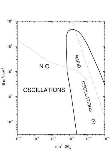
Figure 24: Region of parameter space where the final sign does and does not oscillate for $\nu_{\tau}\leftrightarrow\nu_{s}$ oscillations, according to ref. [652]

This figure should be compared with the calculations based on thermally averaged equations [660] which show that a very large part of parameter space is chaotic, in contradiction to ref. [652] (see fig. 25).

Figure 25: The distribution of the final sign of neutrino asymmetry in the mixing parameter space. Negative signs of $L$ are plotted in black and positive ones are in white. The initial asymmetry was chosen to be $L^{\rm in}=10^{-10}$.

The analytical solution of ref. [658] does not show any chaoticity. To be more precise, numerical solution of equation (384) is chaotic for large values of $K\sin 2\theta$. However this chaoticity is related to numerical instability because with the increasing coefficient in front of the r.h.s. of the equation, the minimal value of the asymmetry becomes very small and can be smaller than the accuracy of computation. In this case the calculated value of the asymmetry may chaotically change sign. However this regime is well described analytically and it can be seen that the sign of asymmetry does not change.

The chaotic behavior observed in the papers [659]-[663] has always been present in a simplified approach the kinetic equations were solved for a fixed “average” value of neutrino momentum, $y=3.15$, so that the integro-differential kinetic equations are approximated by much simpler ordinary differential ones. However, many essential features of the process become obscured in this approach, in particular the “running of the resonance” over neutrino spectrum, and it is difficult to judge how reliable the results are. Moreover, the average value of $1/y$ that enters the refraction index is $\langle 1/y\rangle\approx 1$, and not $1/\langle y\rangle\approx 0.3$, though this numerical difference might not be important for the conclusion.

Possibly fixed-momentum approach is not adequate to the problem, as can be seen from the following very simple example. Let us consider oscillations between $\nu_{a}$ and $\nu_{s}$ in vacuum. Then the leptonic charge in active neutrino sector would oscillate with a very large frequency, $\sim\sin(\delta m^{2}t/E)$, for a neutrino with a fixed energy $E$. However if one averages this result with thermal neutrino spectrum, the oscillations of leptonic charge would be exponentially suppressed. Still this counter-example is also oversimplified and cannot be considered a rigorous argument against chaoticity. It may happen, for example, that for smaller $K$, when saddle point does not give a good approximation, the differential asymmetry $\Delta(q,y)$ may be an oscillating function but the integrated (total) asymmetry is smooth. Another logical option is that for a smaller $K$ the integrated asymmetry is also chaotic but not large. However, one cannot exclude a large asymmetry with a small $K$. It is possible that the fixed momentum approach has an advantage of simplicity and by using this approach one could discover important properties that remain obscured in more accurate methods. Very recently there appeared the paper [664] where a numerical solution of complete momentum dependent kinetic equations was performed. The authors state that they have found chaotic behavior of the solution. This statement contradicts analytical results of ref. [658]. It is difficult to make a final judgment at this stage.

12.6 Active-active neutrino oscillations.

In the previous sections we considered oscillations between active and sterile neutrinos. Oscillations between active ones usually do not lead to modifications of the standard picture because the oscillating partners are well in thermal equilibrium and their density matrices do not evolve, remaining of the same equilibrium form as in the case of no oscillations. However, initial neutrino states might be out of equilibrium and in that case oscillations between active partners could produce interesting effects. We will consider here a scenario where one of the active neutrino flavors has a large initial charge asymmetry, which could be created by processes with leptonic charge non-conservation in the very early universe. Examples of models leading to such state are discussed in secs. 7,10. So the initial state at the moment when oscillations become active could be e.g. a state with a large asymmetry in the sector, say, $\nu_{\mu}$ or $\nu_{\tau}$ and zero asymmetry in $\nu_{e}$. If there is mixing between $\nu_{e}$ and $\nu_{\mu}$ (or $\nu_{\tau}$) then part of muon asymmetry could be transformed through these oscillations into electronic asymmetry. The latter could have a noticeable impact on BBN.

Oscillations between active and sterile neutrinos in the presence of a large lepton asymmetry would be strongly suppressed because the contribution of large asymmetry into neutrino effective potential (305) makes the mixing angle in vacuum negligibly small. This is not true for oscillations between active neutrinos. As was noticed in ref. [606] and discussed in detail in series of papers [639]-[644] the effective potential of oscillating active neutrinos is a non-diagonal matrix in flavor space. The non-diagonal terms are induced by self-interaction of oscillating neutrinos. The presence of non-diagonal terms strongly alters the oscillation pattern. In particular, in this case the oscillations are no longer inhibited by a large charge asymmetry of the plasma and neutrinos with all momenta oscillate as a single ensemble. Some more surprising results were presented - in particular, it was argued that under certain conditions the neutrino gas that initially consisted only of $\nu_{e}$ would go into pure muonic neutrinos and not, as one would expect, into equilibrium state, equally consisting of $\nu_{e}$ and $\nu_{\mu}$. Another surprising statement is that coherence may not be lost thanks to non-linearity of the system. Possible CP-odd effects in neutrino oscillations, as well as neutrino evolution in the presence of initial non-zero chemical potentials also have been discussed in the papers cited above. A clear description of some of these phenomena was presented recently in the paper [678].

As we have already mentioned oscillations between active neutrinos would be unobservable if neutrinos are in complete thermal equilibrium. However neutrino spectrum deviates from equilibrium due to $e^{+}e^{-}$-annihilation following neutrino decoupling [134, 135] (see sec. 4.2). Oscillations could change the distorted spectrum and might be in principle observable in BBN [620]. This effect was considered in ref. [642] and recently in ref. [679]. According to the calculations of the latter the primordial abundance of ${}^{4}He$ changes only by $1.5\cdot 10^{-4}$.

The kinetic equations used in the previous section can be easily modified to apply to this case. Let us consider for definiteness oscillations between $\nu_{e}$ and $\nu_{\mu}$. One has to take into account the self-interaction processes $\nu_{e}\nu_{\mu}\leftrightarrow\nu_{e}\nu_{\mu}$ and $\nu_{e}\bar{\nu}_{e}\leftrightarrow\nu_{\mu}\bar{\nu}_{\mu}$. The refraction index is determined by the forward scattering amplitude and since $\nu_{e}$ and $\nu_{\mu}$ are considered to be different states of the same particle one has to include both processes when there is a $\nu_{e}$ with momentum $p_{1}$ in initial state and a $\nu_{e}$ or $\nu_{\mu}$ with the same momentum in the final state. The processes of forward transformation $\nu_{e}\leftrightarrow\nu_{\mu}$ give non-diagonal contributions to refraction index. Such transformations always exist, even among non-oscillating particles, but only in the case of non-vanishing mixing the non-diagonal terms in the effective potential become observable.

Now instead of expression (287) we have to use

$$H_{int}^{(e,\mu)}=\delta E\left(\begin{array}[]{cc}h_{ee}&h_{e\mu}\\ h_{\mu e}&h_{\mu\mu}\end{array}\right)\equiv{\delta E\over 2}\left(h_{0}+{\bf\sigma\,h}\right)$$ (419)

where $\delta E=\delta m^{2}/2E$ and ${\bf\sigma}$ are Pauli matrices.

It is convenient to present the density matrix as:

$$\rho={1\over 2}\left(P_{0}+{\bf\sigma\,P}\right)={1\over 2}\left(\begin{array}[]{cc}P_{0}+P_{z}&P_{x}-iP_{y}\\ P_{x}+iP_{y}&P_{0}-P_{z}\end{array}\right).$$ (422)

The elements of the Hamiltonian matrix (419) are expressed through the integrals over momenta of the distribution functions of other leptons in the plasma and, in particular, of the elements of the density matrix of oscillating neutrinos themselves. The latter contribute to non-diagonal matrix elements of the Hamiltonian. The structure of these terms is essentially the same as the one discussed above for mixing between active and scalar neutrinos, see eq. (305). The contribution of self-interaction of neutrinos and antineutrinos also contains two terms. One originates from non-locality of weak interactions and is symmetric with respect to charge conjugation:

$${\bf h}_{+}={V_{sym}\over 2\pi^{2}}\int dyy^{3}\left({\bf P}+\bar{\bf P}\right).$$ (423)

The second is proportional to the charge asymmetry in the plasma and equals

$${\bf h}_{-}={V_{asym}\over 2\pi^{2}}\int dyy^{2}\left({\bf P}-\bar{\bf P}\right)$$ (424)

One can find details e.g. in ref. [612]. An essential feature, specific for oscillations between active neutrinos, is the presence of non-diagonal terms in the Hamiltonian (or in refraction index). In the case of large lepton asymmetry in the sector of oscillating neutrinos, the asymmetric terms in the Hamiltonian strongly dominate and, as a result, the suppression of mixing angle in the medium, found for $(\nu_{a}-\nu_{s})$-oscillations, disappears.

If the coherence breaking terms have the simplified form (311) the kinetic equations for density matrix become:

$$P^{\prime}_{0} = -\gamma_{e}\left({P_{0}+P_{z}\over 2}-f_{e}\right)-\gamma_{\mu}\left({P_{0}-P_{z}\over 2}-f_{\mu}\right)$$ (425)

$$P^{\prime}_{x} = -P_{y}(c_{2}+h_{z})+P_{z}h_{y}-P_{x}\gamma_{e\mu}$$ (426)

$$P^{\prime}_{y} = P_{x}(c_{2}+h_{z})-P_{z}(s_{2}+h_{x})-P_{y}\gamma_{e\mu}$$ (427)

$$P^{\prime}_{z} = s_{2}P_{y}+(P_{y}h_{x}-P_{x}h_{y})-\gamma_{e}\left({P_{0}+P_{z}\over 2}-f_{e}\right)+\gamma_{\mu}\left({P_{0}-P_{z}\over 2}-f_{\mu}\right)$$ (428)

where $P^{\prime}_{j}=(Hx/\delta E)\partial_{x}P_{j}$ and the “time” variable $x$ is defined according to eq. (55), $c_{2}=\cos 2\theta$, $s_{2}=\sin 2\theta$, $\theta$ is the vacuum mixing angle, $f_{e,\mu}$ are equilibrium distribution functions with possibly different chemical potentials for $\nu_{e}$ and $\nu_{\mu}$, $\gamma_{a}$ is the damping coefficient for $\nu_{e}$ or $\nu_{\mu}$ normalized to $\delta E$ (see eq. (319)), and $\gamma_{e\mu}=(\gamma_{e}+\gamma_{\mu})/2$.

If the temperature is sufficiently high and thus $\gamma$ is non-negligible, these equations can be accurately solved in stationary point approximation:

$$P_{x}=P_{z}\,{(s_{2}+h_{x})(c_{2}+h_{z})+\gamma_{e\mu}h_{y}\over(c_{2}+h_{z})^{2}+\gamma^{2}_{e\mu}}\approx P_{z}\,{h_{x}\over h_{z}}+\epsilon_{x}$$ (429)

$$P_{y}=P_{z}\,{(c_{2}+h_{z})h_{y}-\gamma_{e\mu}(s_{2}+h_{x})\over(c_{2}+h_{z})^{2}+\gamma^{2}_{e\mu}}\approx P_{z}\,{h_{y}\over h_{z}}+\epsilon_{y}$$ (430)

where $\epsilon_{j}$ are small corrections satisfying $\int dy\,y^{2}(\epsilon-\bar{\epsilon})=0$.

Substituting these expressions into equations (426-428) and integrating over momentum we find:

$$h_{x}=h_{z}\,{s_{2}c_{2}\over c_{2}^{2}+\langle\gamma_{e\mu}\rangle^{2}},\,\,\,h_{y}=-h_{z}\,{s_{2}\langle\gamma_{e\mu}\rangle\over c_{2}^{2}+\langle\gamma_{e\mu}\rangle^{2}}$$ (431)

where $\langle...\rangle$ means thermal averaging. Substituting these expressions into eq. (428) we obtain

$$P^{\prime}_{z}=-P_{z}\,{s_{2}^{2}\gamma_{e\mu}\over c_{2}^{2}+\langle\gamma\rangle^{2}_{e\mu}}-\gamma_{e}\left({P_{0}+P_{z}\over 2}-f_{e}\right)+\gamma_{\mu}\left({P_{0}-P_{z}\over 2}-f_{\mu}\right)$$ (432)

An analogous equation exists for antiparticles. We can further simplify these equations if we assume $\gamma_{e}=\gamma_{\mu}$. In this approximation $P_{0}$ disappears and we arrive at a complete set of equations containing only $P_{z}$ and $\bar{P}_{z}$.

The equilibrium distribution functions $f_{e,\mu}$ depend upon the chemical potentials $\xi_{\nu_{e}}$ or $\xi_{\nu_{\mu}}$. They can be expressed through the lepton asymmetries $(n_{\nu_{a}}-n_{\bar{\nu}_{a}})$. If the asymmetries are large (compared to the “natural” value, $\sim 10^{-9}n_{\gamma}$), then the $z$-component of the Hamiltonian is proportional to the difference:

$$(L_{\nu_{e}}-L_{\nu_{\mu}})\sim h_{z}\sim\int d^{3}y(P_{z}-\bar{P}_{z})$$ (433)

If the coherence breaking term in eq. (432) is sufficiently large, $P_{z}$ should be close to its equilibrium value, with running chemical potentials, $P_{z}\approx P_{z}^{(eq)}\equiv(f_{e}-f_{\mu})$. However, one cannot neglect the last term in eq. (432) because the small difference $P_{z}-P_{z}^{(eq)}$ is multiplied by a large factor $\gamma$. The coherence breaking terms disappear if one subtracts from eq. (432) the corresponding equation for antiparticles and integrate the difference over momentum. This follows from separate conservation of electronic and muonic charges by the coherence breaking terms. This conservation permits to impose an evident relation between $\gamma$ and $\bar{\gamma}$. Taking this difference and integrating over momentum we obtain in the Boltzmann approximation:

$$h^{\prime}_{z}=-{1\over 2}\,h_{z}\,\int d^{3}y\,e^{-y}\,{s_{2}^{2}\gamma_{e}\over\langle\gamma_{e}\rangle^{2}+c^{2}_{2}}$$ (434)

This equation is rather accurate at sufficiently high temperatures, when coherence breaking terms are non-negligible and $c_{2}^{2}$ is not too small. Otherwise stationary point approximation would be invalid.

The solution of this equation is straightforward. It shows that oscillations are not suppressed by matter effects in the presence of large lepton asymmetry.

A detailed numerical investigation of oscillations between three active neutrinos in the early universe is carried out in the paper [306]. An analysis of the impact of oscillating neutrinos on BBN was performed for the values of oscillation parameters favored by the solar and atmospheric neutrino anomalies. For the large mixing angle (LMA) solution flavor equilibrium is established in the early universe and all chemical potentials $\xi_{e,\mu,\tau}$ acquire equal values. The results of the calculations for this case are presented in fig. 26.

Figure 26: Evolution of neutrino chemical potentials for LMA case, $\theta_{13}=0$, and initial values $\xi_{e}=\xi_{\tau}=0$ and $\xi_{\mu}=-0.1$. Solid and dotted curves are obtained with and without neutrino self-interactions respectively.

Since for these values of the parameters, asymmetries in muonic and tauonic sectors are efficiently transformed into electronic asymmetry, the BBN bounds on chemical potentials are quite strong, $|\xi_{a}|<0.07$ for any flavor $a=e,\mu,\tau$.

For the LOW mixing angle solution, the efficiency of the transformation of muon or tauon asymmetries into electronic one is not so efficient. The transformation started at $T<1$ MeV below interesting range for BBN. The results of calculations are presented in fig. 27.

Figure 27: Evolution of the neutrino degeneracy parameters for LOW case and the initial values $\xi_{e}=\xi_{\tau}=0$ and $\xi_{\mu}=-0.1$. Notations are the same as in fig. 26.

The results presented in these figures are valid for vanishing mixing angle $\theta_{13}$ (in the standard parameterization of the $3\times 3$-mixing matrix. An analysis of different non-zero values of $\theta_{13}$ can be found in the paper [306].

12.7 Spatial fluctuations of lepton asymmetry.

A very interesting phenomenon was found in ref. [301]. Neutrino oscillations in the presence of initially small baryonic inhomogeneities could give rise to domains with different signs of lepton asymmetry. This effect is different from the chaotic amplification of asymmetry discussed above. As is shown in section 12.5.3 the initial asymmetry first drops to an exponentially small value and after that starts to rise, also exponentially, with a larger integrated exponent. Since the value of the asymmetry at its lowest could be extremely small, it is sensitive to small perturbations, which could determine the final sign of the asymmetry. This does not go in a trivial way as e.g. spatial fluctuations of the sign in the minimum but in a somewhat trickier manner as will be explained below. As is argued in the original paper [301] (see also ref. [666]), though small spatial fluctuations of the cosmological baryon asymmetry do not create a change of sign at the minimum, they would induce the formation of a domain with super-horizon sizes (at the moment of their creation) with large lepton asymmetries of different signs. The fluctuations of the charge asymmetry themselves are not directly essential - one can see from the results of secs. 12.5.3 that the final sign of the asymmetry is the same as the initial one, if chaoticity (sec. 12.5.4) is not present. However, initial isocurvature perturbations in the background asymmetry, which enters the refraction index of neutrinos (306,307), would induce neutrino diffusion and the diffusion term might have different signs in different space points. According to the arguments of ref. [301], it may dominate the contribution of the background asymmetry in the minimum and generate a sign difference in the final large value of the lepton asymmetry. We will show below how it works.

This effect would have an important impact on BBN and on the subsequent neutrino oscillations. This phenomenon was further studied in ref. [666] in frameworks of a one-dimensional model with momentum-averaged kinetic equations. The authors argued that due to this effect the entire parameter range where the exponential growth of lepton asymmetry takes place is excluded by BBN. In particular, the production of sterile neutrinos through MSW resonance at the domain boundaries (with varying density of leptonic charge) is so strong that it would invalidate the results of refs. [648]-[650].

Let us consider the equation, modeling evolution of the lepton asymmetry in the presence of small spatial inhomogeneities, used in ref. [301]. Following the notations of this paper, let us denote the asymmetry of active neutrinos of flavor $a$ as $L_{\nu_{a}}$. The combination that enters the refraction index of $\nu_{a}$ is $2L_{\nu_{a}}+\tilde{L}$, where $\tilde{L}$ consists of the contributions of other neutrino species, baryons, and electrons. Due to electric charge neutrality, the last two are not independent. Preexisting fluctuations in neutrino asymmetry would be erased due to a large neutrino mean free path in cosmic plasma after neutrino decoupling. So background asymmetry can be written as $\tilde{L}=\bar{L}+\delta B(\vec{x})$, where the first term is homogeneous and the last could be inhomogeneous and related to the fluctuations in the baryon number. The evolution of the neutrino asymmetry is described by the equation:

$$\dot{L}_{\nu_{\alpha}}(\vec{x},t)=a(t)\left[2\,L_{\nu_{\alpha}}(\vec{x},t)+\bar{L}+\delta B(\vec{x})\right]+D(t)\nabla^{2}L_{\nu_{\alpha}}(\vec{x},t)$$ (435)

where $D(t)$ is the diffusion coefficient, and the function $a(t)$ is initially negative and generates an exponential decrease of the asymmetry, but at some critical time $t_{c}$ it changes sign and thus creates a huge rise of the asymmetry. It is essential that, while $a(t)$ is negative, the asymmetry drops down to a very small value. In a more accurate formulation $a$ would also depend on the asymmetry itself, but in what follows we are interested in rather small values of the asymmetry, where non-linear effects are not important.

The solution to this equation can be found by the Fourier transform and we obtain:

$$L_{\nu_{\alpha}}(x,t) = \bar{L}\,\int_{t_{\rm in}}^{t}dt^{\prime}\,a(t^{\prime})\,e^{2\int_{t^{\prime}}^{t}\,dt^{\prime\prime}\,a(t^{\prime\prime})}+$$

$$+ e^{2\,\int_{t_{\rm in}}^{t}dt^{\prime}\,a(t^{\prime})}\int\,d^{3}k\,e^{i{\vec{k}}{\vec{x}}}\,\hat{L}_{\nu_{a}}({\vec{k}},t_{\rm in})\,e^{-k^{2}\,\int_{t_{\rm in}}^{t}dt^{\prime}\,D(t^{\prime})}+$$

$$+ \int_{t_{\rm in}}^{t}dt^{\prime}\,a(t^{\prime})\,e^{2\int_{t^{\prime}}^{t}\,dt^{\prime\prime}\,a(t^{\prime\prime})}\,\int\,d^{3}k\,e^{i{\vec{k}}{\vec{x}}}\,\delta\hat{B}({\vec{k}},t_{\rm in})\,e^{-k^{2}\,\int_{t^{\prime}}^{t}dt^{\prime\prime}\,D(t^{\prime\prime})}$$

Here “hut” indicates the Fourier transform of the corresponding function. The first term in this expression can be explicitly integrated because the integration measure $dt^{\prime}a(t^{\prime})$ is exactly the differential of the exponential. The integration of this term gives:

$$(1/2)\bar{L}\left[\exp\left(2\int^{t}_{t_{in}}dt_{2}a(t_{2})\right)-1\right]$$ (437)

So we obtained a rising term (after some initial decrease) plus a constant initial value of $\bar{L}$.

The second term can be also integrated because the initial value $\hat{L}({\vec{k}},t_{\rm in})$ is supposed to be homogeneous and so its Fourier transform is just delta-function, $\delta^{3}(k)$. The integral gives

$$L_{\nu_{a}}^{(in)}\,\exp\left(2\int^{t}_{t_{in}}dt_{2}a(t_{2})\right)$$ (438)

where $L_{\nu_{a}}^{(in)}$ means the initial value, i.e. taken at $t=t_{in}$. So if we forget about the constant term $\bar{L}/2$, we would have $(L_{\nu_{a}}^{(in)}+\bar{L}/2)$ multiplied by the rising exponent. One would get exactly this expression if one solves the equation for $\dot{L}_{\nu_{a}}$ in the homogeneous case.

Let us now consider the last term which, according to the arguments of ref. [301], could change the sign of the rising asymmetry, i.e. this last term could become the dominant one. To evaluate the integral let us substitute:

$$\delta\hat{B}({\vec{k}},t_{\rm in})=\int d^{3}x_{1}e^{i{\vec{k}}{\vec{x}}_{1}}\,\delta B({\vec{x}}_{1})$$ (439)

where $\delta B({\vec{x}}_{1})$ is the initial value of the inhomogeneous term. Now we can integrate over $d^{3}k$. We have the integral of the type

$$\int d^{3}k\exp[-S^{2}k^{2}+i{\vec{k}}(\vec{x}-{\vec{x}}_{1})]$$ (440)

the scalar product of vectors $\vec{k}$ and $\vec{r}=\vec{x}-\vec{x}_{1}$ is equal to ${\vec{k}}({\vec{x}}-{\vec{x}_{1}})=kr\cos\theta$, and

$$S^{2}(t)=\int_{t_{in}}^{t}dt_{2}D(t_{2})$$ (441)

Integration over angles in $d^{3}k=2\pi k^{2}dkd(\cos\theta)$ is trivial, it gives $\sin kr/kr$. The remaining integration can be done as follows:

$$\int dkk\sin kr\exp[-S^{2}k^{2}]=(d/dr)\int dk\cos kr\exp[-S^{2}k^{2}]$$ (442)

and the remaining integration can be performed if we expand the range of integration from minus to plus infinity. Introducing a new variable $\vec{x}_{1}=\vec{x}-S(t_{1})\vec{\rho}$ we finally obtain

$$\int dt_{1}a(t_{1})\,e^{2\int_{t_{1}}^{t}dt_{2}a(t_{2})}\int d^{3}\rho\,\delta B(\vec{x}-S(t_{1})\vec{\rho})\,e^{-\rho^{2}}$$ (443)

This is the contribution the lepton asymmetry $L_{\nu_{a}}$ generated by the (small) baryonic inhomogeneities. Its asymptotic rise at large $t$ is similar to the rise of other terms, but its exponential decrease at intermediate stage could be considerably milder. As a result, this term could become dominant with the sign determined by the sign of the fluctuations in the baryon asymmetry. We can see this in a simple example assuming that the function $a(t)$ has the form $a(t)=a_{1}(t-t_{c})$ and that the fluctuations of the asymmetry are described by one harmonic mode: $\delta B({\vec{x}})=\epsilon_{B}\cos{\vec{k}_{0}}{\vec{x}}$. This form of $\delta B$ could be inserted either into eq. (443) or into initial eq. (12.7) and we find for the oscillating part of the asymmetry (up to a constant coefficient):

$$\delta L({\vec{x}}) = a_{1}\epsilon_{B}\cos{\vec{k}_{0}}{\vec{x}}\,\,e^{a_{1}(t-t_{c})^{2}-S^{2}(t)\,k_{0}^{2}}\left[\int_{t_{c}-t_{in}}^{t-t_{c}}dt_{1}t_{1}e^{-a_{1}t_{1}^{2}+S^{2}(t_{1})\,k_{0}^{2}}+\right.$$ (444)

$$\left.\int_{0}^{t_{c}-t_{in}}dt_{1}t_{1}e^{-a_{1}t_{1}^{2}}\left(e^{S^{2}(t_{1})\,k_{0}^{2}}-e^{-S^{2}(t_{1})\,k_{0}^{2}}\right)\right]$$

Both terms rise as $\exp[a_{1}(t-t_{c})^{2}]$, i.e. in the same way as the other homogeneous terms (we assume that $S(t)$ is finite at large $t$ and not too large). The first term is exponentially suppressed as $\exp[-a_{1}(t_{c}-t_{in})^{2}]$ also at the same level as the homogeneous terms. The second term, which vanishes in the homogeneous case ( $k_{0}=0$ or $S=0$) is not exponentially suppressed. In the limit of a large $a_{1}$ the integral can be evaluated as $\sim S^{2}(0)\,k_{0}^{2}/a_{1}$. It is small but not exponentially small. Thus, one can easily imagine a situation when the last term dominates and the resonance enhancement of lepton asymmetry in the background of small fluctuations of baryon asymmetry could create domains with large and different lepton asymmetry. The effect is very interesting and deserves more consideration.

Chaotic diffusion of neutrinos from these domains would generate electric currents by scattering of neutrino flux on electrons or positrons in primeval plasma. These currents, in turn, would create cosmic magnetic fields which could serve as seeds of coherent galactic magnetic fields [667].

12.8 Neutrino oscillations and big bang nucleosynthesis.

There are several effects through which neutrino oscillations may have influenced primordial abundances of light elements (we will speak here mostly about mixing between active and sterile neutrinos):

1. If sterile neutrinos are created by oscillations before active neutrino decoupling, then the effective number of neutrino species at nucleosynthesis would be larger than 3. This effect, as is well known, results in an increase of mass fraction of helium-4 and deuterium. If the oscillations were efficient after decoupling of active neutrinos, then the total number density, active + sterile, would remain unchanged and the effect on BBN of $\nu_{\mu}-\nu_{s}$ or $\nu_{\tau}-\nu_{s}$ mixing would be absent. On the other hand, for the mixing between $\nu_{e}$ and $\nu_{s}$, if excitation of sterile neutrinos took place after $\nu_{e}$ decoupling, the production of $\nu_{s}$ would be accompanied by the corresponding decrease in the number/energy density of $\nu_{e}$. This in turn would result in a higher temperature of $n/p$-freezing and also in a larger mass fraction of ${}^{4}He$, though the total energy density of all neutrinos would remain the same as in the standard model.

2. Oscillations may distort the spectrum of neutrinos and, in particular, of electronic neutrinos. The sign of the effect differs, depending on the form of spectral distortion. A deficit of electronic neutrinos at high energy results in a smaller mass fraction of helium-4, while a deficit of $\nu_{e}$ at low energy works in the opposite direction. A decrease of total number/energy density of $\nu_{e}$ (as discussed in the previous point) would result in an earlier freezing of neutrino-to-proton ratio and in a larger fraction of helium-4.

3. Oscillations may create an asymmetry between $\nu_{e}$ and anti-$\nu_{e}$. If the spectra of $\nu_{e}$ and $\bar{\nu}_{e}$ have the equilibrium form with a non-zero chemical potential then the $n/p$ ratio would change as $n/p\sim\exp(-\mu_{\nu_{e}}/T)$. Present day data permit the asymmetry in the sector of electronic neutrinos to be at the level of a few per cent (see sec. 10.3), i.e. much larger than the standard $10^{-10}$. In reality the generation of charge asymmetry by oscillations may strongly distort the spectrum of active neutrinos, in particular, of $\nu_{e}$, and a more complicated analysis is necessary. Even if asymmetry was strongly amplified or if it was a primordial one but still remained below 0.01, its direct influence on BBN would be negligible. It may, however, have an impact on nucleosynthesis in an indirect way. Namely, the asymmetry that is larger by several orders of magnitude than the standard one, could suppress neutrino oscillations through refraction index so that new neutrino species corresponding to sterile neutrinos would not be efficiently excited and/or the spectrum of $\nu_{e}$ would not be distorted.

Thus, one can see that the effects of oscillations may result either in a reduction or an increase of primordial abundances of ${}^{4}He$ and $D$. This effect is usually described by the effective number of neutrino species, though the latter is different for ${}^{4}He$ and $D$. The impact on ${}^{7}Li$ is more complicated.

Historically, the study of the impact of oscillating neutrinos was honed with time, as additional effects were taken into account and more precise calculations were performed. In ref. [54] only excitation of extra neutrino species by oscillations was considered. It was assumed that neutrinos have both Dirac and Majorana masses and and therefore sterile states could be produced through oscillations. The condition that only one extra neutrino species is permitted by BBN prompted the conclusion that the mixing angle should be smaller than 0.01 and/or mass difference cannot be larger than $10^{-6}$ eV². However, the refraction of neutrinos in the primeval plasma was neglected, and thus the results of paper [54] were valid only for a sufficiently large mass difference, $\delta m^{2}>({\rm keV})^{2}$. The refraction index of neutrinos [621] was correctly taken into account in the paper [622], where the probability of excitation of sterile states by oscillations was calculated. The paper mostly considered the non-resonant case. Consideration of resonance was postponed for the subsequent paper [626]. Still it was mentioned in [622] that resonance oscillations might have a strong impact on the lepton asymmetry in the active neutrino sector and could even change the sign of the neutrino asymmetry.

The probability of non-resonant production of sterile neutrinos was first estimated in ref. [622] where the following expression was presented:

$$\Gamma_{s}=\langle\sin^{2}2\theta_{m}\sin^{2}\left(t\omega_{osc}\right)\Gamma_{a}\rangle$$ (445)

Here $\Gamma_{a}$ is the production rate of ordinary (active) neutrinos in the primeval plasma and the averaging is made over the thermal cosmic background. The mixing angle $\theta_{m}$ and the frequency of oscillations in the medium $\delta E$ are given respectively by eqs. (332) and (327). This frequency is normally very high so one can substitute $\sin^{2}(\delta E\,t)=1/2$. The rate of active neutrino production can be parameterized as

$${\Gamma_{a}/H}=\left({T/T_{a}}\right)^{3}$$ (446)

where $H$ is the Hubble parameter and $T_{a}$ is the freezing temperature of the active neutrinos of flavor $a=e,\,\mu,\,\tau$. For $T<T_{a}$ the production of $\nu_{a}$ is effectively switched off. Using this and other expressions above we conclude that the equilibrium of sterile neutrinos is not established [622] for:

$$\sin^{4}2\theta|\delta m^{2}|\leq 6\cdot 10^{-3}{\rm eV}^{2}\left(T_{a}/3\,{\rm MeV}\right)^{6}$$ (447)

If BBN permits $\Delta N_{\nu}<1$ additional effective neutrino species the r.h.s. of this bound would be smaller by the factor $(\Delta N)^{2}$. The values of the freezing temperature taken in ref. [622] were $T_{\nu_{e}}=3$ MeV and $T_{\nu_{\mu},\nu_{\tau}}=5$ MeV. They correspond to the freezing of (inverse) annihilation $l\,\bar{l}\rightarrow\nu\,\bar{\nu}$, where $l$ is a light lepton (electron or any active neutrino). As we saw in sec. 12.4 this is not so and the limit is underestimated.

The other groups [623]-[627], [627]- [629], [632] used formally the same result (445) but argued that the total rate of reactions with active neutrinos should be substituted for $\Gamma_{a}$. The latter is approximately an order of magnitude larger than the annihilation rate and the corresponding limit would be much stronger. The argument in favor of this choice was that sterile neutrinos were produced in any reaction with a related active $\nu$ and not only by inverse annihilation. On the other hand, it is evident that pure oscillations conserve the total number $n_{\nu_{a}}+n_{\nu_{s}}$, as well as elastic scattering does. If no new active neutrinos are produced by some inelastic processes, this conservation law remains intact and the effective number of neutrino species at BBN is not changed by the oscillations. However, if the bulk of sterile neutrinos is produced at sufficiently high temperatures, when annihilation is in equilibrium, then active neutrino states are quickly re-populated by inverse annihilation and the rate of their production is proportional to the total neutrino reaction rate as is argued in the papers quoted above. According e.g. to ref. [116] the limits are $\delta m^{2}\sin^{4}2\theta<5\cdot 10^{-6}\Delta N^{2}_{\nu}$ for $\nu_{e}$ and $\delta m^{2}\sin^{4}2\theta<3\cdot 10^{-6}\Delta N_{\nu}^{2}$ for $\nu_{\mu,\tau}$.

A somewhat more accurate treatment of kinetic equations  (314-317) reveals that in all the estimates made in the previous literature the factor 1/2 has been omitted in the rate of production of $\nu_{s}$ (see eq. (333)). A correction by this factor makes the bounds 4 times weaker. The solution of kinetic equations made in sec 12.4 under assumption of kinetic equilibrium of active neutrinos leads to the bound which is weaker than the quoted ones by another factor 1.5 (so that the total factor is 6). The last discrepancy is not too large and may be explained by different approximations made in the solutions.

A surprisingly strong and different in power of $\sin^{2}\theta$ limit was claimed in ref. [280]: $\delta m^{2}\sin^{2}2\theta<1.6\cdot 10^{-6}$. The authors argued that the probability of creation of sterile neutrinos is proportional to $(\Gamma_{W}/H)^{2}$ in contrast to the usually obtained first power of this factor. This discrepancy is probably related to misinterpretation of the conversion probability versus total probability of production found in ref. [280].

There is a continuing activity in the field and more bounds for different special cases are obtained. The limits on oscillation parameters that were found in the papers. [116, 629, 632] were reconsidered (and relaxed) in ref. [633] for the case of high primordial deuterium. Nucleosynthesis constraints on the oscillation parameters in a concrete model of four-neutrino mixing (three active and one sterile) were considered in refs. [634]-[637]. The values of the parameters were taken in the range indicated by the direct experimental and solar neutrino data, e.i. $\delta m^{2}_{21}\sim 10^{-5}{\rm eV}^{2}$,    $\delta m^{2}_{43}\sim 10^{-2}{\rm eV}^{2}$, and $\delta m^{2}_{31}\sim 1{\rm eV}^{2}$. Complexities due to possible resonance transitions and the related rise of lepton asymmetry were disregarded. Because of that the results could be applicable only to non-resonance signs of mass differences. The effective rate of active neutrino production included both inverse annihilation and elastic scattering, however, as we argued above, the results should be reconsidered for the weaker production rate by the factor 1/2.

It is worth noticing that the bounds are obtained under the assumption that active neutrinos have standard weak interaction. In the case of additional stronger interactions, the refraction index of neutrinos would be larger and the oscillations in the medium would be more strongly suppressed. For example, in the case of additional coupling of neutrinos to majorons the limits discussed above are relaxed by several orders of magnitude [630] and sterile neutrinos would not be dangerous for BBN. Similar arguments were presented recently in ref. [631].

If oscillations take place between $\nu_{e}$ and $\nu_{s}$, another effect may be important [622]: if the equilibrium is not reached, the number density of $\nu_{e}$ would be depleted because of transformation into $\nu_{s}$ after $\nu_{e}$ decoupled from the cosmic plasma. This is turn would result in an earlier freezing of neutron-proton transformations and in a larger $n/p$-ratio. This effect permits to exclude small values of the mass difference, down to $10^{-7}$ eV², for large mixing angles, $\sin^{2}2\theta>0.4$. However the spectrum distortion of electronic neutrinos caused by oscillations was neglected in derivation of this bound; this effect is discussed below.

Resonance oscillations of neutrinos were considered in the early papers [623]-[632] in adiabatic approximation. In refs. [623, 627] it was argued that the oscillations drive lepton asymmetry in active neutrino sector down to zero independently of the existence of resonance transition. This result disagrees with with refs. [622, 626]. In the second of these papers it was found that lepton asymmetry is exponentially unstable with respect to oscillations and is not driven to zero but, on the opposite, is enhanced. Another interesting effect mentioned in ref. [622] is a possible parametric resonance phenomenon in neutrino oscillations in medium. In the case of resonance oscillations the parameter space excluded by BBN is significantly larger and surprisingly the results of the papers [625],[626], and [632] are rather close to each other. For $\sin^{2}2\theta>({\rm a\,\,few\,})\cdot 10^{-2}$ the mass difference above $2\cdot 10^{-7}\,{\rm eV}^{2}$ is excluded; for a smaller mixing the limit is roughly $\sin^{4}2\theta\delta m^{2}\geq 5\cdot 10^{-10}{\rm eV}^{2}$. However, one should take these results with great caution because the simplifications made in the calculations may be non-adequate for the resonance case. A very essential approximation that strongly simplified the calculations was the use of thermally averaged kinetic equations. In this case, instead of infinitely many modes for different neutrino momenta, all matrix elements of neutrino density matrix were taken at the average momentum $\langle p\approx 3T\rangle$. Hence instead of integro-differential equation containing an integral over $d^{3}p$ from neutrino distributions, which is especially important for the charge asymmetry term in the refraction index, one got a much simpler set of ordinary differential equations. However, spectral effects are of primary importance and the average approach could be misleading. A detailed derivation of quantum kinetic equations and an analysis of applicability of momentum-averaged approach can be found in ref. [638].

Unfortunately in the early papers the oscillations were considered in one mode approximation, when all relevant quantities were averaged over neutrino spectrum, as we have already mentioned above. This permits reducing the problem to the functions of one variable - time - instead of both time and momentum. Of course in the frameworks of this formalism one cannot even pose the question about the real spectrum of neutrinos. First works that did not make this simplifying assumption, where the elements of density matrix depending of both variables $p$ and $t$ were considered, were done in refs. [530]-[672]. Kinetic equations governing evolution of density matrix of oscillating neutrinos were numerically solved for relatively small mass difference, $\delta m^{2}\leq 10^{-7}$ eV² and arbitrary vacuum mixing angle. Such small mass difference allows the following simplifications: 1) the effect of coherence breaking are not important, so one could use eqs. (314-317) without damping terms; 2) a small value of $\delta m^{2}$ results in a small oscillation frequency and this stabilizes computations; for a larger $\delta m^{2}$ a significant numerical instability appears.

The authors noticed an important role of the distortion of the spectrum of electronic neutrinos by the oscillations as well as the effect of depletion of $\nu_{e}$ by transformation into $\nu_{s}$ on BBN. According to their observation the spectrum distortion cannot be adequately described by the shifting of the effective neutrino temperature. The analytical fit to the bound on the oscillation parameters that follows from the consideration of primordial ${}^{4}He$ can be written as [671]:

$$\delta m^{2}\,\left(\sin^{2}2\theta\right)^{4}\leq 1.5\cdot 10^{-9}\,\,{\rm eV}^{2},\,\,\,{\rm for}\,\,\,\delta m^{2}<10^{-7}\,{\rm eV}^{2}.$$ (448)

The evolution of lepton asymmetry due to oscillations was studied both for resonant and non-resonant cases. In the non-resonant case the initially small asymmetry, i.e. of the order of the baryonic one, remains unnoticeable for nucleosynthesis [668]. In the resonant case the asymmetry might be considerably amplified by the resonance transition. An analysis of ${}^{4}He$-production in the presence of neutrino oscillations with a small mass difference, $\delta m^{2}<10^{-7}$ eV² was performed recently in ref. [680]. It was shown that the mass fraction of ${}^{4}He$ may increase up to 14% in non-resonance case and up to 32% in the resonance case.

The impact of the amplification of the asymmetry on BBN for a larger mass difference has been studied in refs. [647]-[650], [653]. In the case of $(\nu_{e}-\nu_{s})$-mixing the impact of asymmetry generation on BBN is very strong and the result depends upon the final sign of the asymmetry in $\nu_{e}-\bar{\nu}_{e}$ sector. If the asymmetry is negative so that $n_{\nu_{e}}<n_{\bar{\nu}_{e}}$, the mass fraction of the produced ${}^{4}He$ increases. This corresponds to a positive contribution to the number of effective neutrino species. In the opposite case the effect is negative. The magnitude of this contribution into $N^{(eff)}_{\nu}$, according to the calculations of ref. [653], as a function of mass difference is presented in fig. 28.

Figure 28: Change in the effective number of neutrino species for BBN, $\Delta N_{\nu}$ versus $-\delta m^{2}$ for the case $\sin^{2}2\theta=10^{-8}$ and $L_{\nu_{e}}>0$, according to ref. [653]

In the case of more complicated mixing between all active neutrinos and one sterile $\nu$ (which is necessary to explain all neutrino anomalies) the process of asymmetry generation in $\nu_{e}$-sector might proceed in two stages [647, 648, 533]. First, a large $\nu_{\tau}$-asymmetry was generated by the resonance transition $\bar{\nu}_{\tau}-\bar{\nu}_{s}$. At the second stage, the oscillations $\bar{\nu}_{\tau}-\bar{\nu}_{e}$ created some asymmetry in $\nu_{e}-\bar{\nu}_{e}$ sector. As was argued in ref. [647] for the model with $m_{\nu_{\tau}}\gg m_{\nu_{\mu},\nu_{e},\nu_{s}}$ the net result is either $N^{(eff)}_{\nu}=3.4$ or $N^{(eff)}_{\nu}=2.5$ in a rather wide range of mass difference, $\delta m^{2}=10-3000$ eV². In ref. [648] a different mass pattern was considered: $m_{\nu_{\tau}}\sim m_{\nu_{\mu}}\gg m_{\nu_{e},\nu_{s}}$ with the mixing angles favored by the experimental data. In this case, according to ref. [648], $N^{(eff)}_{\nu}=3.1$ or $2.7$. The mirror universe model with three extra mirror neutrinos mixed with three “our” ones is considered in ref. [533]. A bigger freedom of the model permits to explain the atmospheric neutrino anomaly by $(\nu_{\mu}-\nu_{\mu}^{\prime})$-mixing (where $\nu_{\mu}^{\prime}$ is the mirror muon neutrino) without distorting successful prediction of BBN. The number of extra neutrino species in the model can change from (-1) to (+1). The results of these works disagree with ref. [681] where it was argued that the $\nu_{\mu}-\nu_{s}$ solution to the Super Kamiokande data [45, 46] could evade the BBN bounds only for a very large mass difference, $200{\rm eV}^{2}<\delta m^{2}<10^{4}{\rm eV}^{2}$. It was also argued in this paper [681] that the effects of time variation of neutrino asymmetry and non-instantaneous repopulation would strongly change the BBN limits found in the papers [647, 648]. On the other hand, the calculations of refs. [647, 648] were re-examined in the work [650], where it was found that the corrected results are in rough agreement with the earlier papers [647, 648] and the corrections are not crucial. Some more discussion of the problem can be found in refs. [682, 683]. All the groups at least agree that the Super Kamiokande data [45, 46] on atmospheric neutrino anomaly in principle could be compatible with BBN in the resonance case when a large lepton asymmetry in $\nu_{e}$-sector are generated, while it is not so if asymmetry is small [648, 681].

As we have already mentioned the new data from SNO and SuperKamiokande experiments disfavor pure active-sterile neutrino mixing (see however [55]). An analysis of four neutrino mixing of $2+2$ and $3+1$ types has been performed recently in ref. [186]. It has been shown there that in both schemes sterile neutrinos are completely excited in the plasma and $\Delta N_{\nu}=1$. According to the same paper, this result in the case of small lepton asymmetry contradicts the combined BBN + CMBR data which permit only $\Delta N_{\nu}<0.3$. A possible way out is to suggest another sterile neutrino with such a mixing that allows to generate a noticeable electron neutrino asymmetry.

The effect on BBN of primordial lepton asymmetry, considerably larger than $10^{-10}$ in $\nu_{e}$ sector, was analyzed in refs. [669, 670] for small mass differences, $|\delta m^{2}|<10^{-7}$ eV². While in the absence of oscillations, BBN is sensitive only to asymmetry at the level above $10^{-2}$, much smaller values of asymmetry become important if oscillations take place. The effect is indirect - the asymmetry changes the light element production through its influence on neutrino oscillations and they, in turn, change number density and spectrum of active neutrinos. The asymmetry in the range $10^{-7}<|L|<5\cdot 10^{-6}$ has a complicated impact on the oscillations. It could either enhance or suppress oscillations depending on the concrete values of the parameters. Thus the restrictions on the values of $\delta m^{2}$, $\sin 2\theta$, and $L$ could be either weaker or stronger. Smaller $|L|$ have very little influence on BBN, while $|L|$ larger than $5\cdot 10^{-6}$ strongly suppresses the oscillations. These results can be only obtained if complete (not thermally averaged) equations are used. As is argued in these works, in the case of $\delta m^{2}>0$, when the “averaged” resonance transition is absent, there could be a resonance, say, in neutrino transition but only for a certain momentum value. This transition can change the lepton number and after some time the resonance condition for neutrinos ceases to be fulfilled, but becomes valid for antineutrinos. So the process proceeds through “alternating” resonances. Of course this phenomenon would be lost after thermal averaging.

A hot dispute arose between two groups [684, 685] and [669, 670] in connection with the role of lepton asymmetry in oscillations and BBN. Though one cannot say that there is direct contradiction between them because the oscillations are considered in non-overlapping range of parameters, $\delta m^{2}<10^{-7}$ eV² in ref. [669] and $\delta m^{2}\sim 10^{-2}-10^{3}$ eV² in ref. [684], some qualitative difference between the conclusions of the two groups can be found. An advantage of the calculations [669] is an exact numerical solution of kinetic equations for each momentum mode (see discussion above), in contrast to an approximate approach of the group [684], who works in the parameter region where numerical calculations are much more complicated. More work in this direction is definitely in order.

Possibly the case of a large mixing angle, $\sin 2\theta>10^{-3}$ and a large mass differences $\delta m^{2}\sim{\rm eV}^{2}$ can be treated rather reliably even in approximate resonance approach [686, 687] (compare with sec. 12.5). The authors considered the parameter range favored by the existing experimental indications on neutrino oscillations. They found a large suppression in the low energy part of the spectrum of both neutrinos and antineutrinos relative to the thermal distribution and showed that this spectral distortion has an impact on primordial ${}^{4}He$ at the level of several per cent - which is within a range sensitive to observational constraints.

A recent review of some of the problems discussed in this subsection can be found in ref. [688].

12.9 Summary

Although great progress has been made in understanding the physics of neutrino oscillations in the early universe, still a few unsettled problems remain. The case of small mass difference, $|\delta m^{2}|\leq 10^{-7}$ eV² is relatively simple. The oscillations in this case became effective late enough to allow neglecting the loss of coherence and the repopulation of active neutrinos. Numerical solutions [530]-[672] look stable and sufficiently accurate.

The approximate treatment of the non-resonant case and the corresponding bounds on the oscillation parameters from BBN in principle does not create any serious problem, though all the papers have missed the factor $1/2$ in the estimate of production rate of sterile neutrinos (333,445). The disagreement between the works [622] and subsequent ones [116, 629, 632] on whether the rate of reproduction of active/sterile neutrinos should include only inverse annihilation or elastic scattering as well (see discussion in secs. 12.4,12.8) is resolved in favor of the later papers but the BBN bounds on the oscillation parameters are between the results of ref. [622] and refs. [116, 629, 632], because according to the calculations of sec. 12.4 the correct bound is weaker by factor 6, from which factor 4 is explained by the missed factor 1/2 mentioned above and the origin of the other 1.5 is unclear.

The huge rise of lepton asymmetry [298] up to 0.375 in the resonance case is confirmed by several different methods [298],[645]-[654], [658] and can be very interesting for BBN [653]. An important unresolved issue related to the rising asymmetry is its possible chaotic, oscillating behavior. It was observed in the papers [659]-[664], [681]-[687] and is not supported by other cited in sec. 12.5.4. The difficulty of the numerical approach is that the integral of the charge asymmetric diagonal part of the density matrix over momentum (373) contains quickly oscillating functions and enters kinetic equations with a large coefficient. Hence it is difficult to separate the real oscillating behavior from numerical artifacts. The effect of chaoticity was definitely observed in the framework of the simplified thermally averaged equations but was not seen or proven within the exact momentum dependent ones, except for the recent work [664]. On the other hand, chaoticity might appear in the range of parameters where neither analytical methods nor numerical ones are applicable.

Oscillations among active neutrinos do not lead to noticeable effects in BBN if initial lepton asymmetries are small. If it is not so, the asymmetries would be equilibrated in the case of the LMA solution and the BBN bound on neutrino degeneracy would be more restrictive than that without oscillations. For the LOW solution the impact of neutrino oscillations on BBN is much weaker (sec. 12.6).

13 Neutrino balls.

A very interesting phenomenon may take place in left-right symmetric electro-weak theory. Since usually the left-right symmetry is assumed to be spontaneously broken, and so right-handed bosons and right-handed Majorana neutrinos are very heavy over our “left” vacuum, while they are light over “right” vacuum, and, vice versa, our neutrinos that are light over our vacuum are heavy over “right” vacuum state. However, if the symmetry breaking was spontaneous, but not explicit, these two vacuum states would be degenerate. As a result of a phase transition in the early universe mostly the left vacuum state was formed (at least in the visible part of the universe. However, small bubbles of another, right, vacuum state might also remain. Models leading to such an apparent violation of left-right symmetry can be built, but we will not go into detail here. Discussion and reference can be found in the papers [689, 690, 691]. The small bubbles of wrong (i.e. “right”) vacuum remaining after hot cosmological epoch could be stable or, to be more exact, long-lived and could have survived to the present day. They form quasi-stable non-topological solitons, or so called neutrino balls [689], supported against collapse by the pressure of right-handed neutrinos that are light inside the ball and heavy outside. Thus the wall between two vacuum states is impenetrable for neutrinos, while it is transparent for electrons, positrons and photons that are common for the left-handed and right-handed worlds.

The pressure exerted by the surface tension

$$p_{st}=2\sigma/R,$$ (449)

where $\sigma$ is the surface energy density and $R$ is the radius of the ball, should be balanced by the pressure of the neutrino gas inside the ball. The mass of the ball consists of the mass of the wall separating the two vacua and the mass of neutrino gas inside:

$$M_{ball}=4\pi R^{2}\sigma+{4\over 3}{6\sigma\over R}\pi R^{3}=12\pi R^{2}\sigma$$ (450)

When the radius of a ball enters cosmological horizon micro-physical processes inside the ball determine its evolution. Typically, cosmological expansion is turned into contraction forced by the surface tension. The neutrino gas inside becomes degenerate with the chemical potential (the same for neutrinos and antineutrinos) equal to [689, 690]:

$$\mu\approx 0.15\,{\rm MeV}\,\sigma_{{\rm TeV}}^{3/8}M_{6}^{-1/8}$$ (451)

where $\sigma_{{\rm TeV}}=\sigma/{\rm TeV}^{3}$, $M_{6}=M_{ball}/10^{6}M_{\odot}$, and $M_{\odot}=1.99\cdot 10^{33}$ g is the solar mass. The equilibrium radius of such a ball is

$$R_{eq}=3\cdot 10^{12}\,{\rm cm}\,M_{6}^{1/2}\sigma_{{\rm TeV}}^{-1/2}$$ (452)

If the ball mass is greater than $10^{8}M_{\odot}\sigma_{{\rm TeV}}^{-1}$, the equilibrium radius is smaller than the gravitational radius and such balls would form primordial black holes and exist forever. Neutrino balls with masses below $10^{4}M_{\odot}\sigma_{{\rm TeV}}^{3}$ would be very short-lived due to the process $\nu_{R}\bar{\nu}_{R}\rightarrow e^{-}e^{+}$. For heavier balls and correspondingly for $\mu<m_{e}$ this process is energetically impossible and other weaker mechanisms of burning would be essential. The process $\nu_{R}\bar{\nu}_{R}\rightarrow 2\gamma$ proceeds only in the second order in weak interaction [692] and is negligible. The reaction $\nu_{R}\bar{\nu}_{R}\rightarrow 3\gamma$ would burn the balls out during the time [689]:

$$\tau_{3\gamma}=10^{14}\,\left(m_{e}/\mu\right)^{13}\,{\rm sec}$$ (453)

Another possible reaction that could destroy the ball is

$$\nu_{R}\bar{\nu}_{R}e\rightarrow e\gamma.$$ (454)

It gives the life-time [690]:

$$\tau_{\gamma}=4\cdot 10^{21}\left(m_{e}\over\mu\right)^{4}\left(1\,{\rm eV}^{3}\over n_{e}\right)\,{\rm sec}$$ (455)

where $n_{e}$ is the electron number density inside the ball. Normally this process is sub-dominant with respect to $3\gamma$-burning but matter accretion on neutrino balls could create a much larger number density of electrons, up to [691] $n_{e}=10^{9}\sigma_{{\rm TeV}}^{3/2}M_{6}^{-1/2}\,{\rm eV}^{3}$. In fact the number density should be somewhat smaller because the matter accretion must stop when the ball reaches critical (Eddington) luminosity. In this scenario neutrino balls remain stable for a long period - practically until the present time - and then emit their mass during 10-100 million years emitting about 0.1 solar mass per year.

Some further studies of the properties of neutrino balls, with gravity effects taken into account, can be found in the papers [693, 694, 695]. Properties of neutrino balls in a supersymmetric model are considered in ref. [696].

Possible cosmological and astrophysical implications of these objects are rather interesting. Firstly, they could form primordial black holes if their mass exceeds the value $10^{8}M_{\odot}/\sigma_{{\rm TeV}}$. The latter could be seeds for galaxy formation. For smaller masses they are unstable and may have luminosity close to that of quasars. This opens a competing mechanism for the central engine of quasars [690, 691, 693] instead of the canonical one by the accretion of matter on a superheavy black hole. Possibly both mechanisms could be operating and heavy neutrino balls that formed black holes are active galactic nuclei (and heavy quasars), while the lighter ones are (or better to say, were) short-lived quasars that can be observed only in distant parts of the sky (at relatively large red-shifts).

As argued in ref. [697], neutrino balls could present a viable model for gamma bursters if a supernova were captured by a ball and exploded inside. However, more probable is a capture of an ordinary or neutron star by a neutrino ball. This captured matter could create a strong outburst of energy by the reactions similar to (454).

The term “neutrino balls” (or “neutrino stars”) was later used in the literature [700]-[708] in a very different content. Namely it was assumed that massive neutrinos could form gravitationally bound stellar-like structures and the works focused on the properties and implications of such objects. Although it is possible that non-relativistic self-gravitating neutrinos may form stable stellar mass (or million stellar mass) objects, the mechanism of their formation is unclear. It is a difficult problem to form a gravitationally binded system at stellar scale from dissipationless particles. This problem is addressed in a recent paper [708], where authors argue that “dissipationless formation of a heavy neutrino star in gravitational collapse is numerically demonstrated”. The value of neutrino mass assumed in the models is about 10 keV, so an additional annihilation mechanism must be introduced to avoid contradiction with Gerstein-Zeldovich bound. This can be achieved by an anomalous neutrino interaction with a new light boson. Such new, stronger-than-weak, interaction could also aid the formation of a gravitationally bound system of heavy neutrinos, helping with energy dissipation. Massive neutrinos with 10 keV mass that escaped capture into neutrino stars, could form halo of dark matter around different astronomical objects and, in particular, around the Sun. Possible observational manifestation of this form of dark matter are discussed in ref. [706].

The massive object in the center of our Galaxy (Sgr A^∗) may possibly be identified with a neutrino ball. Normally it is assumed that the Galaxy hosts a supermassive black hole with the mass about $3\cdot 10^{6}\,M_{\odot}$. This hypothesis implies the luminosity close to $10^{41}$ erg/sec but the observed luminosity from radio to $\gamma$-ray frequencies is below $10^{37}$ erg/sec. A possible way to solve this problem is to assume that the object in the galactic center is a gravitationally bound system of massive neutrinos discussed in the previous paragraph. This hypothesis was recently analyzed in ref. [709], where it was found that to satisfy astrophysical constraints, the neutrino mass should be in a rather narrow interval: $11\,\,{\rm keV}<m_{\nu}<24\,\,{\rm keV}$.

14 Mirror neutrinos.

The idea that there may exist another world, which communicates with ours through gravity and possibly, though not necessarily, through some other very weak interaction, has a long history. After it became known that CP-parity is broken [710], Kobzarev, Okun, and Pomeranchuk [711] suggested that invariance with respect to a modified CP reflection could be restored if the particle content of the theory is doubled, i.e. there exist two parallel worlds, ours and the mirror one, related by a new generalized CP-transformation. Of course, if these worlds communicate/interact in any way they should have common gravitational interaction. An analysis of other possible interactions, that could connect the two worlds, was performed in ref. [711]. It was shown that, in addition to gravity, mirror particles might possibly be connected to us only through some new very weak, weaker than normal weak, interaction. In the same paper [711] a possible existence and detection of macroscopic astronomical bodies consisting of mirror matter were discussed. Later, in 1980’s Okun [712] considered a possibility that an interaction between the two worlds might be not very weak if it proceeded through an exchange of new neutral mesons.

Another type of particle doubling was assumed in ref. [713] in an attempt to explain the decays seen by Cronin et al [710] without breaking CP by introducing shadow K-mesons and other shadow particles. It was proposed in this paper that the two worlds were not symmetric, the mirror symmetry was broken and the properties of ours and mirror, or now better to say, shadow particles were different.

A possibility of some particle doubling was mentioned in the paper by Lee and Yang [714], where parity violation was proposed. The authors suggested that parity might remain an exact symmetry of the theory if, in addition to left-handed protons of our world, there exist mirror symmetric protons, so in a broad sense there is left-right symmetry in the Lagrangian. In this picture the observed right-left asymmetry is prescribed to a local preponderance of, say, left-handed protons over right-handed ones. According to ref. [714], the interactions between $p_{R}$ and $p_{L}$ is not necessarily weak and they might interact with the same electromagnetic and even the same pion fields, but it was later shown [711] that this could not be true.

The hypothesis of mirror (shadow) particles/universe was later elaborated in many papers [715]. An interesting implication of the idea of a mirror world is the possibility of explaining the smallness of neutrino mass [716, 717] by an analog of see-saw mechanism (see sec. 16).

As was suggested in two pioneering papers, there are two possible types of scenarios of parallel worlds: the first is the case of exact symmetry between the worlds, so that the physics there is identical to ours and the other one is the case of different physics, which could be due to a different pattern of symmetry breaking in the two worlds. The first version is often called the exact parity symmetry or mirror case, while the second one is referred to as a shadow universe.

Cosmological implications of the existence of another practically sterile (except for gravity and possibly very weak interactions) universe, especially in connection with dark matter, were considered in many papers [718], but in what follows we will concentrate only on those which are related to neutrino physics. In a model with a broken mirror symmetry [534, 535] the scale of electroweak symmetry breaking in the shadow world was taken to be 30 times larger than our electroweak scale. Correspondingly shadow neutrinos would be about 1000 (i.e. $30^{2}$) times heavier than our neutrinos, and if the latter have the mass in eV range the former could have keV mass and contribute to warm dark matter (see sec. 11). Due to asymmetric inflationary reheating that could give different temperatures to our and the shadow worlds, the number density of the heavy shadow neutrinos would be sufficiently small to avoid a contradiction with the Gerstein-Zeldovich limit. Smaller temperature of the shadow world would make it non-dangerous at BBN as well.

In the model of refs. [534, 535] interactions between the worlds, in addition to gravity, proceeds through mixing between neutrinos, so the shadow neutrinos would be perceived in our universe as sterile neutrinos slightly mixed with the active ones. This idea was proposed earlier in refs. [719, 720] in the framework of the exact parity model. In a simultaneous paper [721] it was argued that even if the original coupling between the worlds was only due to gravity, quantum gravity effects on the Planck scale would induce mixing between our and mirror neutrinos. Thus, the mixing between neutrinos in the two worlds is inevitable or, at least, quite natural and they would be produced in the early universe through coherent oscillations that are discussed in sec. 12, and where the BBN bound on the oscillation parameters are presented.

The implications of mirror neutrinos for the early universe cosmology in the exact parity models are considered in detail in ref. [533], see also [722]. In the simplest versions of these models one would expect that the cosmological energy density of mirror particles and ours should be equal. In particular, they should be equal at BBN. The contribution of mirror particles in this case corresponds to the effective number of neutrino species slightly over 9, and is definitely excluded (see sec. 6). However, in the case of resonance oscillations between ours and mirror neutrinos a large lepton, especially electron, asymmetry can be generated in our world (see secs. 12.5, 12.8). This asymmetry would have a strong impact on BBN, either enlarging or diminishing the effective number of neutrino species. The analysis of oscillations including 3 active and 3 sterile flavors was performed in ref. [533] (for the earlier work see ref. [723]), where it was shown that the exact parity model was consistent with BBN for a large region of the oscillation parameter space. On the other hand, even in the case of exact mirror symmetry in the Lagrangian, the cosmological evolution of the different worlds could be different (a kind of spontaneous symmetry breaking) and the energy density of mirror particles might be much smaller than ours.

15 Neutrino and large extra dimensions.

It was suggested several years ago [240] that the characteristic scale of gravity might be a few TeV instead of the usual Planck scale $10^{19}$ GeV. This could be realized if there are extra dimensions in addition to the usual $3+1$. The Standard Model (SM) fields live in the $(3+1)$-dimensional brane, while gravity and possibly some other fields could propagate in the bulk including the brane plus additional dimensions. The latter are compact and the compactification scale could be as large as a fraction of mm. The standard left-handed neutrinos localized in the bulk could mix with SM-singlet fermions propagating in the bulk [724]-[729] and would be interpreted in our world as sterile neutrinos. In the model of refs. [726, 730] the mass of active neutrinos and the non-diagonal matrix elements of the mass matrix are determined by one free parameter, $m_{i}$, while the diagonal entries for the bulk neutrinos are equal to $n/R$, where $R$ is the size of the extra dimensional manifold. According to ref. [730] the mass matrix of mixed bulk and brane neutrinos has the form:

$$M_{i}=\pmatrix{m_{i}&\sqrt{2}m_{i}&\sqrt{2}m_{i}&\cdots\cr 0&1/R&0&\cdots\cr 0&0&2/R&\cdots\cr\vdots&\vdots&\vdots&\ddots}$$ (456)

The model describes one active neutrino with mass $m_{\nu_{a}}$ and the infinite tower of sterile ones with the masses $n/R$ and mixing angles essentially given by $\sin\theta\sim m_{\nu_{a}}R$ (if the latter is small, $m_{\nu}R\ll 1$). For details see e.g. ref. [730].

The infinite tower of sterile neutrinos might be dangerous for BBN. This problem was sketched in ref. [730], where it was argued that the effect of these $\nu_{s}$ is not catastrophically large and even might be compatible with BBN. The essential point on which this conclusion is based is that the mixing angle diminishes with the rising number of excitation, $n$, so the effect of all the tower on BBN is at most as that of one neutrino species. An accurate treatment demands solving the infinite system of the coupled kinetic equations for the density matrix, and that has not yet been done.

A more extensive analysis was carried out in ref. [731], where not only BBN but also data on CMBR, structure formation and diffuse photon background were taken into consideration. The effective number of neutrino species at BBN corresponding to $j$-th Kaluza-Klein (KK) excitation of the bulk neutrinos, analytically estimated in this work, is

$$\Delta N_{\nu_{j}}\sim 10^{-3}\left({m_{\nu}\over 1\,\,{\rm eV}}\right)^{2}\left({g_{*}^{f}\over g_{*k}^{p}}\right)$$ (457)

where $m_{\nu}$ is the active neutrino mass, and the last factor approximates the dilution effect caused by the ratio of relativistic species at the active neutrino decoupling and at the maximum production of the Kaluza-Klein mode $j$. The temperature of the latter is approximately: $T_{max}=133\,\,{\rm MeV}\,\,(m_{j}/1\,{\rm keV})^{1/3}$ (see eq. (351)). The result (457) noticeably differs from that of ref. [730] and more work is desirable to resolve the controversy.

Taken together, the cosmological constraints discussed in ref. [731] deal a serious blow to the simple model of bulk neutrinos mixed with the usual active ones. However, as the authors noted there could be simple modifications of the models that might allow circumventing the constraints. First, the mixing angle and life-time of KK neutrinos are model dependent and it is possible to modify the particle physics framework to avoid contradictions with cosmology. Second, the result depends upon the geometry of the bulk. In particular, the compactification would not necessarily be toroidal one or there might be additional branes in the bulk that could change the decay properties of heavier neutrinos. Thus cosmology can definitely restrict certain models of sterile neutrinos coming from large extra dimensions, but at the present time it cannot rule out the general idea.

The BBN constraints on the models with large extra dimensions [730, 731] have been derived for the case of $\geq$ 2 extra dimensions. In ref. [732] the models with one extra dimension and with the string scale $\sim 10^{9}$ GeV have been studied. It was shown there that such models are compatible with BBN and the mixing of bulk to active neutrinos is in the range interesting for solar neutrino oscillations.

16 Neutrinos and lepto/baryogenesis.

If cosmological baryon asymmetry originated from previously created lepton asymmetry [733], one can obtain quite restrictive bounds on neutrino mass in many realistic models of particle physics. In short, the idea is as follows. It is believed that sphaleron processes [734], operating above the electroweak phase transition, would destroy all preexisting cosmological charge density of $(B+L)$. In principle, the same processes could generate $(B+L)$ at lower temperatures when the phase transition was in process. This would require deviations from thermal equilibrium, which could be effective only if the phase transition was first order.

Heavy Higgs makes this option practically excluded. For the reviews see refs. [296], [735]-[738]. If electroweak processes are able only to destroy preexisting asymmetry and not to create one, we would need either low temperature baryogenesis or some mechanisms to create a non-zero $(B-L)$ prior to EW phase transition. This difference, $(B-L)$, is conserved and electroweak processes can transform it into some nonvanishing and generically non-equal lepton and baryon asymmetries (see below, eq. (466)). This way, the observed baryon asymmetry of the universe might be generated. This scenario is reviewed in refs. [739, 740, 741].

A possible mechanism of creation of lepton asymmetry is a decay of a heavy Majorana neutrino [742], $\nu_{M}$. The existence of such a particle permits a natural explanation of the small masses of observed left-handed neutrinos by a mixing with the heavy Majorana companion (the so called see-saw mechanism [743]). Lepton asymmetry, created by out-of-equilibrium decays of heavy $\nu_{M}$, was generated at a period when the rate of lepton charge production:

$$\Gamma_{L}=\Gamma_{M}n_{\nu_{M}}/T^{3}\approx\alpha_{M}m_{M}\exp({-m_{M}/T})(m_{M}/T)^{3/2}$$ (458)

was of the order of the Hubble expansion rate, $H\sim T^{2}/m_{Pl}$. Here we assume that the decay rate of $\nu_{M}$ is equal to $\Gamma_{M}=\alpha_{M}\,m_{M}$. Since the magnitude of the lepton asymmetry should not be smaller than the observed baryon asymmetry we should request that the number density of $\nu_{M}$ must be larger than $10^{-9}$ of the entropy density at the moment of equilibrium breaking, when $T=T_{f}$. It means that $\exp(-m_{M}/T_{f})(m_{M}/T_{f})^{3/2}>10^{-9}$ or $m_{M}>10^{-9}\alpha_{M}(m_{M}/T_{f})^{2}m_{Pl}\sim(10^{8}-10^{10})$ GeV. We have assumed here that the freezing temperature $T_{f}\sim(0.1-0.01)m_{M}$ and $\alpha_{M}\sim 10^{-2}-10^{-4}$. This lower limit on $m_{M}$ can be translated into an upper limit on the mass of light neutrinos because the latter, according to the see-saw mechanism is inversely proportional to $m_{M}$. In this way a very restrictive upper bound $m_{\nu}\sim m_{l}^{2}/m_{M}<3\cdot 10^{-3}$ eV can be obtained (here $m_{l}$ is the charged lepton mass). One should keep in mind, however, that the mass of the heavy Majorana neutrino is strongly model dependent. As argued in ref. [744] the isosinglet Majorana mass may be in the interval from 1 TeV up to grand unification scale depending upon the mechanism of CP violation and the flavor structure of neutrino mass matrix.

Another line of arguments is based on the request that lepton asymmetry, or $(B-L)$, generated at the earlier stage is not destroyed by the simultaneous action of $L$-nonconserving processes and sphaleron interactions. If both types of processes are efficient and thermal equilibrium is established, then both $B$ and $L$ must vanish. The sphaleron interactions are known to be in equilibrium in the temperature interval

$$(T_{EW}\approx 100\,\,{\rm GeV})<T<(T_{SPH}\approx 10^{12}\,\,{\rm GeV}).$$ (459)

In addition to the heavy neutrino decays, leptonic charge non-conservation with $\Delta L=2$ could originate e.g. from the effective coupling of lepton of flavor $i$, ($l_{i}$) and Higgs ($H$) fields (see e.g. [740]):

$${\cal L}_{\Delta L=2}=g_{ij}H^{2}l^{T}_{i}Cl_{j}+\,{\rm h.c.}$$ (460)

This interaction could be generated by the exchange of heavy Majorana neutrino. The Yukawa coupling constants $g_{ij}$ enter the mass matrix of light neutrinos which appears in the phase where the Higgs field acquires a non-vanishing vacuum expectation value, $\langle H\rangle\neq 0$. Hence the rate of reactions with $\Delta L\neq 0$ is proportional to the light neutrino mass squared. From the condition that $B$ and $L$ are not destroyed in the temperature interval (459) we obtain the limit [740]:

$$\sum_{i}m_{\nu_{i}}^{2}<\left[0.2\,{\rm eV}\,\left({T_{SPH}\over T_{B}}\right)^{1/2}\right]^{2}$$ (461)

where $T_{B}$ is the baryogenesis temperature, which is usually taken equal to $T_{B}=T_{EW}=100$ GeV. In the first paper [733] a slightly weaker limit, $m_{\nu}<50$ keV, was derived. The more stringent bound (461) was obtained in ref. [745] where the anomalous non-conservation of fermion number was taken into account at the temperatures above the electro-weak phase transition. In a series of papers [746]-[752] much stronger bounds on neutrino masses than (461) have been derived from the condition of successful baryogenesis in the framework of concrete particle physics models. In particular, if one takes $T_{B}=10^{10}$ GeV which is a typical leptogenesis temperature, the upper limit on the light neutrino mass would be very strong, $m_{\nu}<2$ eV. A more general, model independent limit, similar, to (461) can be found from the condition [753] (for a review see [754]) that the lepton number non-conserving processes $W^{\pm}+W^{\pm}\rightarrow e^{\pm}+e^{\pm}$ at $T\sim m_{W}$ do not wash out lepton charge generated earlier by $\nu_{M}$ decays. In other words the reaction rate should be smaller than the Hubble expansion rate:

$$\Gamma(W\,W\rightarrow l_{i}\,l_{j})={\alpha_{W}^{2}\,\,(m_{\nu})^{2}_{ij}T^{3}\over m_{W}^{4}}<5.44\sqrt{{g_{*}\over 10.75}}\,{T^{2}\over m_{Pl}}$$ (462)

where $l_{i}$ is a charged lepton ($e,\,\mu$ or $\tau$) and $m_{\nu}$ is an entry (not necessary diagonal one) of the Majorana mass matrix of light neutrinos. The reaction rate is estimated at $T\sim m_{W}$ where it has the maximum value. From the condition (462) we find

$$(m_{\nu})<20\,\,{\rm keV}$$ (463)

If the above mentioned conditions are fulfilled, then after the electroweak phase both baryon and lepton asymmetries would be created. Naively one would expect that, since $(B+L)$ is not conserved by sphalerons, then in thermal equilibrium $B+L=0$ or, in other words, $B=-L=(B-L)_{in}/2$. The difference $(B-L)$ is conserved by sphalerons and, as we mentioned above, should be generated at an earlier stage by some other $(B-L)$-non-conserving interactions. However, generally the statement $(B+L)=0$ is not true. Some combinations of non-conserved charges in thermal equilibrium must vanish but this depends upon the particle content of the theory and this vanishing combination is not necessarily $(B+L)$. It can be easily seen from the following example. Let us assume that there is only one generation of left-handed quarks, $u$ and $d$ (which have three colors) and leptons, $(\nu,l)$. There are weak interaction reactions: $u+\bar{d}\leftrightarrow\nu+\bar{l}$ and all crossed ones, where $l$ is a negatively charged lepton. There are also two processes induced by sphalerons which break lepton and baryon numbers: $uudl\leftrightarrow{\rm vacuum}$ and $udd\nu\leftrightarrow{\rm vacuum}$. In a realistic case, the reactions include more particles, but the main features are the same. In equilibrium the following relations between chemical potentials hold:

$$2u+d+l=0,\,\,\,u+2d+\nu=0$$ (464)

where for chemical potentials we use the particle symbols, i.e. $u\equiv\mu_{u}$, etc.

In the case of small chemical potentials the corresponding charge density is a linear function of the potentials, and thus the baryonic, leptonic, and electric charge densities can be written as:

$$B\sim u+d,\,\,\,L\sim l+\nu,\,\,\,{\rm and}\,\,\,Q\sim 2u-d-l$$ (465)

Here we made use of the fact that the baryonic charge of an individual quark is $1/3$ but there are three quark colors having equal chemical potential. Using eqs. (464,465) we easily find $(B+L)=-(B-L)/2$. A realistic case includes right-handed quarks and charged leptons, intermediate bosons, and higgses. It was considered in ref. [745] where the following relations between $B$ and $L$ were obtained:

$$B+L=-{6N+5m\over 22N+13m}\,(B-L),\,\,\,B={8N+4m\over 22N+13m}\,(B-L),$$ (466)

where $N$ is the number of quark-lepton families and $m$ is the number of Higgs doublets.

This result is obtained at high temperatures, above the electroweak phase transition and under the assumption that all particle species are in thermal equilibrium. The latter assumption was critically reanalyzed in refs. [755, 756]. It was found that right-handed electrons could be out of equilibrium because of their small Yukawa coupling to Higgs bosons. On the other hand, anomalous sphaleron interactions are effective only for left-handed particles. Because of that, lepton asymmetry would be preserved in the sector of right-handed electrons and not erased as was suggested in the earlier papers quoted above. This result leads to a significant weakening of the previously found bounds. According to the detailed calculations of ref. [756] the upper limit on the neutrino mass is about 20 keV, an order of magnitude weaker than the earlier estimates by the same authors [755] and we essentially return to (461) with $T_{B}=100$ GeV.

There has been a recent burst of activity in the field, stimulated by the observed neutrino anomalies and a related indication to nonzero neutrino masses. In ref. [757] the scenario of baryo/leptogenesis based on the flipped $SU(5)$ model was considered. In ref. [758] two models with the symmetry groups $SU(5)\times U(1)_{F}$ and $SU(3)_{c}\times SU(3)_{L}\times SU(3)_{R}\times U(1)_{F}$, where $U(1)_{F}$ is the flavor group, were discussed in detail with an accurate solution of kinetic equations governing the evolution of the asymmetry. Relations between leptogenesis, neutrino masses, and (supersymmetric hybrid) inflation were discussed in refs. [759, 760]. Reheating after inflation and related gravitino problem was analyzed in ref. [761]. It was shown that in minimal supersymmetric extension of the standard model, almost all existing scenarios of leptogenesis and neutrino masses, except for the one involving right-handed sterile neutrinos, are ruled out for a large range of gravitino mass. The models with Abelian and discrete family symmetries and their impact on leptogenesis and neutrino masses were studied in ref. [762]. A scenario of baryo/leptogenesis with degenerate neutrinos was further considered in ref. [763]. A modification of see-saw mass equation in left-right symmetric theories with two Higgs triplets was considered in the papers [764]. Baryon asymmetry would be successfully described if neutrino masses are not smaller than $10^{-6}-10^{-8}$ eV.

Further development in this area was related to a modification of the leptogenesis scenario, which did not necessarily proceed through non-equilibrium decays of heavy Majorana neutrinos. Such a new version was proposed in refs. [765, 766]. It was assumed that, instead of right-handed neutrinos, there exist additional heavy Higgs scalars, and lepton number was generated through decays of these new heavy Higgs particles, whose interactions explicitly break lepton number. The model permits the accommodation of light sterile neutrinos strongly mixed with the usual active ones. The masses of neutrinos were taken in eV down to $10^{-3}$ eV range and all neutrino anomalies were explained. It is unclear however, if the BBN constraints can be satisfied and how the new SNO data would change the parameters of the model.

In ref. [767] a left-right symmetric model was considered, where both discussed above possibilities of leptogenesis could be realized. As is shown in the paper, successful leptogenesis requires the mass of the right-handed neutrinos to be quite high, $m_{N}\geq 10^{16}$ GeV, if $m_{N}$ exceeds the mass of right-handed intermediate bosons. However in supergravity models this option is excluded because of the cosmological gravitino problem. The case of $m_{N}<m_{W_{R}}$ is more realistic and could lead to successful leptogenesis.

Successful baryogenesis could proceed even without generating a non-vanishing $(B-L)$, as was necessary for the scenarios discussed above. A model of this kind is presented in ref. [768]. According to the model, either a good old GUT baryogenesis operated at the GUT scale and created a non-zero $(B+L)$ or some other processes generated lepton asymmetry in the left-handed lepton sector which might be compensated by the asymmetry in right-handed neutrino sector. The latter could proceed e.g. in heavy particle decays even without lepton number violation and no heavy Majorana lepton would be necessary. By assumption the decays of heavy bosons create both left- and right-handed quarks and leptons, in particular, $\Phi\rightarrow\bar{l}_{L}+\nu_{R}$. Hence the $(B+L)$-asymmetry or just $L$-asymmetry produced in these decays is shared between left and right handed quarks and leptons. At smaller temperatures sphaleron processes become effective. However right-handed particles do not interact with sphalerons and the total, left plus right, asymmetry could be equilibrated only by the Yukawa coupling of left- and right-handed fermions to Higgs bosons. They would wash out all $(B+L)$ if $(B-L)=0$ and if the Yukawa coupling is sufficiently strong. This is not the case for neutrinos if their mass is smaller than 10 keV (see sec. 6.4). In this case the lepton asymmetry stored in right-handed neutrinos, with Dirac mass, does not communicate with the asymmetry in the sector of left-handed particles. Correspondingly $(B-L)_{L}$ in this sector is non-vanishing and as a result the baryon asymmetry processed by sphalerons becomes non-zero as well, see eq. (466).

A new idea that lepton asymmetry might be produced through CP-violating oscillations of sterile neutrinos was explored in ref. [769]. This asymmetry is then transferred to ordinary neutrinos through their Yukawa coupling with sterile ones. The lepton asymmetry in the active neutrino sector produces baryon asymmetry at electro-weak scale through sphaleron processes, as discussed above. In this model the total lepton number (active plus sterile) is conserved and the redistribution of lepton asymmetry between active and sterile neutrinos leads to generation of baryon asymmetry. An important ingredient is the freezing of sphaleron transformation. Otherwise all asymmetry in the sterile sector would be transformed into the active sector and since $L_{tot}=0$ the net result would be also zero. From the condition that sterile neutrinos decayed before the nucleosynthesis epoch, their mass should be larger than $\sim$GeV. On the other hand, the condition that the Majorana mass does not wash out baryon and lepton asymmetry leads to the upper bound on the mass, $M_{s}\ll 100$ GeV. In the model of ref. [769] it means that the Yukawa coupling constants are bounded by $h^{2}\ll 10^{-10}$ and the mass of active neutrinos, which is given by $m_{a}=h^{2}v^{2}/M_{s}$, should be in the range $m_{a}=(10^{-2}-10^{3})$ eV. Depending upon the version of the scenario this limit could be more restrictive. Two of the active neutrino species would have masses in the range $(10^{-6}-10^{-1})$ eV and the third one might have a mass in eV range and make hot dark matter.

The idea to generate $(B-L)$ through Affleck-Dine mechanism [297] with subsequent electro-weak reprocessing was suggested in the recent paper [770] in a supersymmetric hybrid inflation model. The right-handed neutrino superfield naturally appears in the model to fine-tune dynamically the necessary initial conditions for inflation. According to the model the masses of light neutrinos created by the see-saw mechanism are in the range indicated by the data on neutrino anomalies, if the latter are interpreted as manifestations of neutrino oscillations.

In ref. [771] the idea to generate lepton asymmetry in scattering processes was explored. Usually light particles that efficiently participate in scattering are in thermal equilibrium and no charge asymmetry can be generated. However in the version of ref. [771] leptons of our world communicated with leptons in a hidden sector, e.g. mirror or shadow world (see sec. 14). There is no equilibrium between these worlds and lepton asymmetries in both of them could be generated.

In all the papers described above the characteristic scale of generation of lepton asymmetry was very high, roughly speaking $10^{9}-10^{10}$ GeV or even higher. In ref. [772] the model of low energy leptogenesis was suggested at the expense of extending the standard model of particle physics by adding three right-handed neutrinos with the mass about 10 TeV and two new charged Higgs fields which are singlets under $SU(2)_{L}$. This model operates at the TeV-energies accessible to new accelerators and can be checked in upcoming experiments.

Another possible way of generating small neutrino masses is realized in the Zee model, where the masses are induced by radiative corrections and leptonic charge is broken explicitly [773]. If the non-conservation of leptonic charge in this model is strong at electroweak scale, then both $B$ and $L$ would be washed out. However, as is shown in ref. [774], this is not the case because of the approximate conservation of the difference of lepton numbers $L_{e}-L_{\mu}-L_{\tau}$. Thus earlier generated $B_{L}$ would not be destroyed by the combined action of sphalerons and explicit $L$-nonconserving interaction in the Zee model.

Leptogenesis in theories with large extra dimensions was considered in ref. [775]. It was assumed that in addition to the particles of the standard model localized on the brane, there exists an isosinglet neutrino field living in the bulk (see sec. 15). For compactified extra dimensions this field describes an infinite Kaluza-Klein tower of Dirac neutrinos which, after an introduction of leptonic charge non-conservation, split into pairs of nearly degenerate Majorana neutrinos. Each pair of the Majorana neutrinos presents a strongly mixed two-level system producing a large C- and CP-violation. Lepton asymmetry generated by decays of these Majorana neutrinos could be very big and could transform into baryon asymmetry. For successful implementation of the scenario the universe should be reheated above 5 GeV.

There is a wealth of literature on the subject and many papers on the field may have been omitted here. In specific models of particle physics the upper limits on the masses of light neutrinos could be much more restrictive than those presented in this section. However the bounds are strongly model dependent and sometimes do not have an important impact on cosmology. So we confine our discussion to the presented material. More references can be found in the quoted above papers, especially in the review ones [740, 741, 776].

A few more scenarios relating cosmological baryon asymmetry with neutrino masses have appeared recently [777]-[779]. A supersymmetric model of ref. [777] with additional supermultiplets and with string scale unification at $\sim 10^{13}$ GeV may lead to a cosmological lepton asymmetry through the decay of this heavy superfield and to a conversion of this asymmetry into the observed baryon asymmetry. The masses of light neutrinos arising in this model naturally fit the atmospheric and solar neutrino data. In ref. [778] a general analysis of models of lepto/baryo-genesis at the low energy scale 1-10 TeV is presented. Several known models of leptogenesis are discussed and a new model based on three-body decays of right-handed neutrinos is proposed. The latter allows successful lepto/baryo-genesis and neutrino mass generation at low scale. A relation between the Dirac neutrino mass matrix and the magnitude of the baryon asymmetry is studied in ref. [779]. As is shown in the paper, if the neutrino mass matrix is related to quark or charged lepton mass matrix the baryon asymmetry would be 2-3 orders of magnitude smaller than the observed one. For successful baryogenesis a less pronounced hierarchy of neutrino mass matrix is necessary.

17 Cosmological neutrino background and ultra-high energy cosmic rays.

The observation of ultra high energy cosmic rays (UHECR) with $E>10^{20}$ eV poses a serious problem to the standard theory of the origin and propagation of energetic cosmic particles. At the present day more than twenty such events have been observed by different groups [780]. It is traditionally assumed that the primaries that induce energetic atmospheric showers are protons formed somewhere in violent cosmic sources, e.g. in active galactic nuclei. However such protons cannot come from a very large distance because of the Greisen-Zatsepin-Kuzmin cutoff [781]. Protons with the energy $E>E_{GZK}=5\cdot 10^{19}$ eV strongly interact with CMBR, producing pions in the resonance reaction with the excitation of $\Delta$-isobar: $p+\gamma\rightarrow\Delta\rightarrow N+\pi$, where $N$ is either proton or neutron. The necessary energy for this process can be roughly found from the condition $s\equiv(p_{p}+p_{\gamma})^{2}\sim 2E_{p}E_{\gamma}>2m_{p}m_{\pi}$ which gives a result rather close to $E_{GZK}$ presented above. Due to this inelastic process a proton loses half of its energy at a distance of approximately 20 Mpc. Since no possible sources of high energy cosmic rays are seen in the directions of the primaries of the ultra high energy events up to the distance $\sim 100$ Mpc, and the interstellar magnetic fields are too weak ($<$ a few micro-gauss) to bend protons with such a high energy, the observations [780] present a serious challenge to the standard theory of the origin of UHECR, for a review see [782].

The directions of arrival of cosmic rays with $E>E_{GZK}$ are not correlated with Galactic or Supergalactic plane [780]. Possible sources of the UHECR are more or less uniformly distributed over the sky. However, there are pairs and triplets of UHECR coming from the same direction on the sky within the resolutions of AGASA [824, 793] and Yakutsk (ref. 2 in [780]). This small scale clustering component is statistically significant at the level of 4.5 $\sigma$ and suggests that sources of UHECR are point-like [825, 826]. Another important fact is that events in the clusters have different energy and uncorrelated arrival times. This means that clustered UHECR particles are neutral. Natural candidates for such particles would be photons, however the photons with energies $E\sim 10^{19}-10^{20}$ eV lose energy within 50 Mpc due to creation of $e^{\pm}$ pairs on CMBR and cosmic radio background.

A significant (almost 5 $\sigma$) correlation of UHECR in both AGASA and Yakutsk data with BL Lacertae objects (quasars, with jet beamed in our direction and no strong emission lines in their spectra) found recently in ref. [827] creates even more puzzles. The nearest such objects are located at the distance 150 Mpc ($z=0.03$), well beyond the GZK volume. The largest part of the known BL Lacertae are located at moderate $z\sim 0.1$, or unknown redshifts. If they are indeed the sources of UHECR then they should produce photons with extremely high energies $E>10^{23}$ eV. Such photons could propagate several hundred Mpc, constantly losing energy, and create secondary photons inside the GZK volume. These particles would be the UHECR registered above the GZK cutoff [828]. However, this model requires extremely high energies of primary photons, a very small magnitude of (unknown) extragalactic radio background, and extremely small extra galactic magnetic fields (EGMFs), $B<10^{-12}$ G. Moreover, if the significant correlation with sources at high redshifts, $z>0.2$, is found, this model will be ruled out.

The only known Standard Model particle that is able to travel from high redshift sources, $z\sim 1$, is the neutrino. The mean free path of very energetic neutrinos with respect to the resonance production of $Z$-boson by scattering on the cosmic neutrino background (CNB) is close to the horizon size [783, 784]. To excite the $Z$-resonance the energy of the ultra high energy (UHE) neutrinos should be equal to:

$$E_{UHE}=m_{Z}^{2}/2E_{CNB}\approx 4\cdot 10^{21}\,\,{\rm eV}(1\,\,{\rm eV}/E_{CNB})$$ (467)

where $E_{CNB}$ is the energy of the cosmic background neutrinos. If they are massless then $\langle E_{CNB}\rangle\approx 3T_{\nu}\approx 5\cdot 10^{-4}$ eV. For massive neutrinos with $m_{\nu}>T_{\nu}$, $E_{CNB}=m_{\nu}$.

The energy averaged cross-section is

$$\bar{\sigma}_{Z}=\int(ds/M_{Z}^{2})\sigma(\bar{\nu}\nu\rightarrow Z)=2\pi\sqrt{2}G_{F}=4\cdot 10^{-32}\,{\rm cm}^{2}$$ (468)

Because of the resonant nature of the process the cross-section contains only first power of $G_{F}$ and is much larger than typical weak interaction cross-sections. The mean free path of UHE neutrinos with respect to this reaction is

$$l_{free}=1/(\sigma_{Z}n_{\nu})\approx 5\cdot 10^{29}\,\,{\rm cm}\,(n_{\nu}/55{\rm cm}^{-3})^{-1}\approx 150\,\,{\rm Gpc}\,\,(n_{\nu}/55{\rm cm}^{-3})^{-1}$$ (469)

where $n_{\nu}$ is the neutrino number density; it is normalized to the standard average cosmological number density of neutrinos $n_{\nu}^{(0)}=55/{\rm cm}^{3}$, see eq. (73).

Thus a possible source of ultra high energy cosmic ray events could be the decay of $Z$-boson produced by very energetic neutrinos annihilated on CNB within 100 Mpc. The primary energetic neutrinos could be produced by active galactic nuclei at very large distances. This explanation was suggested in the papers [785, 786]. The $Z$-boson produced in the reaction $\bar{\nu}\nu\rightarrow Z$ would have gamma-factor $\gamma=m_{Z}/2m_{\nu}=4.5\cdot 10^{10}({\rm eV}/m_{\nu})$. The average proton multiplicity in $Z$-decay is 2 and the proton energy in the rest frame of $Z$-boson is roughly 3 GeV. Hence the energy of protons from such a source would be about $1.3\cdot 10^{20}({\rm eV}/m_{\nu})$ eV, which is very close to the registered signal for $m_{\nu}\sim 1$ eV. If this mechanism is indeed operative, the registration of UHECR could mean that the cosmic neutrino background has been discovered. The energetic neutrinos can be considered as messenger fields from distant violent sources.

However, the “Z-burst” mechanism is severely constrained by at least two types of observational data. First, there are upper limits on the UHE neutrino flux, based on non-observation of horizontal air showers by the old Fly’s Eye [829] or by the AGASA [830] experiments and from non-observation of radio pulses that would be emitted from the showers initiated by the UHE neutrinos on the Moon rim [831]. Second, even if the sources exclusively emit neutrinos, the electroweak interactions would also produce photons and electrons initiating electromagnetic (EM) cascades and transferring the injected energy down below the pair production threshold for the energetic photons on CMBR [782]. The cascades would give rise to a diffuse photon flux in the GeV range which is constrained by the flux observed by the EGRET instrument on board of the Compton $\gamma-$ray observatory [832].

The first self-consistent calculation of the Z-burst model was done in ref. [794]. It was assumed there that the distribution of neutrino sources evolves with redshift as $(1+z)^{3}$ or in the way similar to the evolution of active galaxies. It was shown that in this case the secondary photons with energies $E<100$ GeV would overshoot the measured EGRET flux several times. This means that the ”Z-burst” mechanism in its simplest version contradicts the data.

A possible solution to this problem is to increase the local neutrino densities by a factor $N>20$ on scales $l\sim 5$ Mpc [794]. The probability of neutrino interactions would locally increase and for the same flux of UHECR (normalized to the experimental data) the secondary EM flux in the EGRET region of energies would be below the measured values. A development of the local overdensity idea and its different applications were discussed in refs. [787] and [788].

The necessary flux of primary energetic neutrinos, which would excite $Z$-resonance and would agree with the data, depends upon the number density of CNB and the neutrino mass. The cosmological number density of relic neutrinos in the case of vanishing lepton asymmetry is $n_{\nu}^{(0)}=55/{\rm cm}^{3}$. However massive neutrinos could cluster around gravitationally bound astronomical systems and their number density might be much higher. According to estimates presented in ref. [792] the enhancement factors for 1 eV neutrinos are respectively $10^{2}$, $10^{3}$, and $10^{4}$ for galactic supercluster, cluster, and galactic halo. In the subsequent paper [789] the results are approximately an order of magnitude weaker. There is an upper limit to the number density of clustered neutrinos due to their Fermi statistics [483] (see sec. 11.1). The number density of degenerate neutrinos is $n_{\nu}=p_{F}^{3}/6\pi^{2}$, where $p_{F}$ is the Fermi momentum. The average velocity is equal to $\langle V\rangle=p_{F}/4m_{\nu}$. Hence

$${n_{\nu}\over n_{\nu}^{(0)}}\leq 4\cdot 10^{2}\left({m_{\nu}\over{\rm eV}}\right)^{3}\,\left({V\over 200\,{\rm km/sec}}\right)^{3}$$ (470)

where $V$ is the virial velocity, see discussion before eq. (221). This bound does not permit a too-large enhancement of $n_{\nu}$.

The UHE neutrino flux, which is necessary for the explanation of the observed cosmic rays events by the $Z$-burst mechanism, can be estimated as follows. One can see from the AGASA data [793] that the flux of UHECR with $E\sim 10^{20}$ eV is

$$FE^{2}\approx 5{\rm eV/sec/sr/cm}^{2}.$$ (471)

It corresponds to the energy density of the UHECR $\rho_{UHECR}\approx 2\cdot 10^{-9}$ eV/cm³. The rate of production of such energetic cosmic rays can be estimated assuming that they were produced throughout all cosmological time, $t_{c}=1/H$:

$$\dot{\rho}_{UHECR}=H\rho_{UHECR}=0.5\cdot 10^{-26}{\rm{eV\over sec\,cm^{3}}}=0.7\cdot 10^{43}\,\,{{\rm erg\over Mpc^{3}\,\,year}}$$ (472)

Now we have to take into account the fact that these UHECR are secondary, produced by the interaction of $10^{21}$ eV neutrinos with CNB inside roughly 30 Mpc. It means that the energy production rate of the primary UHE neutrinos should be $\sim 10(l_{free}/30\,{\rm Mpc})$ times bigger than $\dot{\rho}_{UHECR}$ (472). It gives

$$\dot{\rho}_{prim}=2\cdot 10^{47}(n_{\nu}^{(0)}/n_{\nu})\,{{\rm erg\over Mpc^{3}\,\,year}}$$ (473)

Such a large rate may require an unusual mechanism of production of UHE neutrinos.

The detailed analysis of constraints on the neutrino flux which came from non-observation of horizontal air-showers was done in ref. [810]. The authors made a comprehensive study of possible observational signatures of energetic neutrinos taking their spectral index and the local neutrino density enhancement as free parameters. It was shown that the existing data on horizontal showers practically exclude clustering of background neutrinos with a small halo size for explanation of the UHECR. Marginal room is left for models with low neutrino mass, $m_{\nu}\sim 0.1$ eV, a very large halo size, about 50 Mpc, and rather flat spectrum with spectral index $\gamma\sim 1.2$. The analysis made in ref. [811] also disfavors the model with clustering of background neutrinos. According to this paper the annihilation of UHE neutrinos on CNB could give no more than 20% of the observed UHECR flux.

An even stronger bound comes from the fact that neutrinos with masses $m_{\nu}<1$ eV are the Hot Dark Matter particles and their distribution is less clustered than the distribution of the total mass [478, 504]. The clustering scale for neutrinos with such a small mass is of the order of the size of clusters of galaxies, i.e. several Mpc. The local CDM distribution is well known on such scales from peculiar velocity measurements and does not allow to have overdensities more than by the factor 3-4 [833, 834]. One could conclude that high overdensities by factor 20 or larger contradict the data.

A possible way to ”reanimate” the Z-burst model was suggested in  [812]. Instead of an unrealistic local neutrino overdensity the model of relic neutrinos with a large neutrino chemical potential was considered. Degenerate neutrinos could have a much larger cosmological number density than the usual $55/$cm³ and the constraints of ref. [810] are not applicable to them. With the concrete value of neutrino mass, $m_{\nu}=0.07$ eV taken from the Super-Kamiokande data on atmospheric neutrinos (see sec. 2) the authors of ref. [812] concluded that the necessary value of neutrino chemical potential should be $\mu_{\nu}=(4-5)\,T$. Unfortunately this value is outside the limits (212) found from CMBR and from BBN bounds for mixed active neutrinos [306] (see sec. 12.6).

One can assume of course that the Z-burst mechanism is responsible only for a part of UHECR  [790]. In this case both primary neutrino and secondary photon fluxes can be reduced to obey all existing limits. However, the origin of the remaining dominant part of UHECR remains mysterious.

Recently a detailed numerical study of the Z-burst model was performed in ref. [835]. The calculations were based on the solution of the Boltzmann transport equations for the spectra of nucleons, $\gamma-$rays, electrons, $\nu_{e}$, $\nu_{\mu}$, $\nu_{\tau}$, and their antiparticles moving along straight lines. Arbitrary injection spectra and redshift distributions of the sources can be substituted into the code and all relevant strong, electromagnetic, and weak interaction reactions can be taken into account [836]. This code was compared on the level of individual reactions with the older version of such code, used in ref. [794]. Contrary to the latter, the code of ref. [835] allows to use arbitrary neutrino masses and distribution of the sources. The neutrino injection spectrum per comoving volume was parametrized as:

$$\phi_{\nu}(E,z) = f(1+z)^{m}\,E^{-q_{\nu}}\Theta(E^{\nu}_{\rm max}-E)\,$$ (474)

$$z_{\rm min}\leq z\leq z_{\rm max}\,,$$

where $f$ is the normalization factor to be fitted from the data. The free parameters are the spectral index $q_{\nu}$, the maximal neutrino energy $E^{\nu}_{\rm max}$, the minimal and maximal redshifts $z_{\rm min}$, $z_{\rm max}$, and the redshift evolution index $m$.

The possibility to vary the distribution of neutrino sources suggested in ref. [835] permitted to avoid the disagreement of the Z-burst model with the data. In order to reduce the photon flux in the EGRET region one can introduce non-uniformly distributed sources more abundant at low redshifts, instead of assuming a local neutrino overdensity. The fluxes of cosmic rays for different values of $m$ are presented in fig. 29. The value $m=3$ corresponding to the spectrum of ref. [794], predicts an excessive photon flux in the EGRET energy region and is excluded by the data. The uniform source distribution, $m=0$, is already in agreement with the EGRET flux, while the negative value, $m=-3$, leads to GeV photon flux well below it. The latter corresponds to the sources which are more abundant now than at high redshifts. For example, the BL Lacertae objects which are correlated with UHECR according to ref. [827], are distributed in such a way.

Figure 29: Fluxes of neutrinos, $\gamma-$rays, and nucleons predicted by the Z-burst mechanism for $m_{\nu}=0.5$ eV, assuming sources exclusively emitting neutrinos with fluxes equal for all flavors  [835]. Three cases of the source evolution parameter, $m=-3,0,3$ are shown by solid, dashed, and dotted lines, respectively. Values assumed for the other parameters are: extragalactic magnetic field strength $B=10^{-9}$ G, minimal radio background strength, $z_{\rm min}=0$, $z_{\rm max}=3$, $E^{\nu}_{\rm max}=2\times 10^{22}$ eV, $q_{\nu}=1$. For each case the neutrino flux amplitude $f$ is obtained from minimizing $\chi^{2}$ for $E_{\rm min}=2.5\times 10^{19}~{}{\rm eV}$. Also shown are experimental upper limits on $\gamma-$ray and neutrino fluxes (see text and Ref. [782] for more details).

If the Z-burst model works one could reverse the arguments and “measure” neutrino mass using the observed spectrum of UHECR because according to eq. (467) the resonance energy in production of $Z$-bosons depends upon $m_{\nu}$ [789]. The main problem in interpretation of the data is that the protons and photons, produced in Z-boson decays, interact with cosmic electromagnetic backgrounds and the observed spectra are very far from those produced by the Z-decays, see fig. 29. Still an upper bound on neutrino mass about a few eV can be found because for neutrinos with higher mass the secondary protons and photons from Z-decay would have energies below the observed UHECR values.

Nevertheless, according to the papers [790, 791] the best fit to the data can be obtained with $m_{\nu}=2.34^{+1.29}_{-0.84}$ eV for the production of UHECR in the Galactic halo and $m_{\nu}=0.26^{+0.20}_{-0.14}$ eV for the extragalactic origin. Later, in ref. [835] was shown that it was possible to obtain the strong results of refs. [790, 791] because many unknown parameters, e.g. neutrino injection spectra eq. (474), were fixed at certain definite values. Moreover, the authors of refs. [790, 791] did not take into account the flux of secondary photons, assuming that all of them were cascaded in energy in the EGRET region. The conclusion of ref. [835] was that the current state of knowledge does not allow to extract any restrictive information on neutrino masses from the UHECR data. The results of refs. [790, 791] were reanalyzed in the recent paper [837] where was found that $m_{\nu}=0.08~{}{\rm eV}-1.3~{}{\rm eV}$ in agreement with the conclusion of ref. [835].

The Z-burst model discussed above is based on the assumption that astrophysical sources emit only neutrinos. However, according to standard scenarios, the UHE neutrinos are secondaries from the interactions of primary accelerated protons. Together with neutrinos the protons produce gamma-rays with approximately the same power as neutrinos (because both neutrinos and photons are secondaries of pion decays). The photon spectrum, typically ends up at the energies $E^{\gamma}_{\rm max}=100\,$TeV [838]. In this case the Z-burst scenario is difficult to make consistent with observations. A possible solution to this problem is to down-scatter most of the EM energy into sub-MeV range within the source. Only if such mechanism is efficient the EGRET bound could be satisfied.

One more problem would appear if the source of high energy particles is not completely opaque to the primary nucleons. Even if a small fraction of them could leave the source, then according to ref. [795], the nucleon flux between $10^{18}\,$eV and $10^{19}\,$eV would be much higher than observed. If the high energy neutrinos are produced in photo-meson or proton-proton interactions in the sources that are not much larger than the mean free path with respect to these reactions then the following upper bound on neutrino flux can be obtained [796, 797]:

$$E^{2}_{\nu}F<2\cdot 10^{-8}{{\rm GeV\over cm^{2}\,sec\,sr}}$$ (475)

This result depends upon the spectrum of primary protons. There are two possible ways to escape this bound, either through production of neutrinos in sources that are optically thick to photo-nucleon and nucleon-nucleon interactions, so the protons are trapped in the sources, or in the processes that do not create simultaneously high energy cosmic rays. Conventional astrophysical sources of this kind are unknown.

Another difficulty of the Z-burst mechanism is the necessity to accelerate primary neutrino producing protons up to energies $E^{p}_{\rm max}\sim 10E^{\nu}_{\rm max}\sim 4\times 10^{22}\,{\rm eV}\,({\rm eV}/m_{\nu})$. On the other hand, known mechanisms are usually limited by $E^{p}_{\rm max}<10^{22}\,$eV [839].

Thus, the Z-burst model imposes the following requirements for the sources [835]: they should emit energy only in neutrinos and, possibly, in sub-MeV $\gamma-$rays and trap most of the primary protons. These protons should be initially accelerated up to very high energies $E^{p}_{\rm max}>10^{22}\,$eV, which requires an unknown acceleration mechanism.

According to the paper [835] the contribution to the UHECR flux from such hypothetical extragalactic neutrino sources due to the Z-burst mechanism would exhibit the GZK-cutoff for nucleons and would be dominated by $\gamma-$rays at higher energies. The required UHE neutrino fluxes are close to the existing upper limits and should be easily detectable by future experiments such as Auger [840], Euso [841], RICE [842], or by other radio detection techniques [843]. Another possibility to observe energetic neutrinos by searching for $\tau$-air showers is discussed in ref. [844].

In view of the difficulties of the Z-burst model discussed above, non-traditional sources of production of UHE neutrinos have been considered, namely superheavy particles or topological defects, which decay predominantly into neutrinos and other invisible particles. In ref. [798] was assumed that there exists a long-lived superheavy relic particles, $X$, with the mass twice larger than the neutrino resonance energy (467). The decays of these particles into neutrino and a light invisible partner could produce the necessary neutrino flux determined by (473) if their mass, life-time, and number density satisfy the condition:

$${n_{X}m_{X}\over\tau_{X}}=\dot{\rho}_{prim}\approx 2\cdot 10^{-22}\left({n_{\nu}^{(0)}\over n_{\nu}}\right){\rm{eV\over sec\,\,cm^{3}}}$$ (476)

Correspondingly $\tau_{X}\sim 0.5\cdot 10^{26}\,\,{\rm sec}\,{\Omega_{X}}h^{2}\left(n_{\nu}/n_{\nu}^{(0)}\right)$. This simple estimate is reasonably close to the results presented in refs. [798, 799].

Both the bound (475) and Fly’s Eye bound (see Fig. 29) are not applicable to the case of neutrinos coming from heavy particle decays because their spectrum is peaked at $E_{\nu}\sim m_{X}$ and is very much different from the neutrino spectrum from traditional astrophysical sources. However, the GLUE bound Fig. 29 still constrains the neutrino flux near its maximum value. The results for proton and photon fluxes presented in the paper [835] are applicable to the model of ref. [798].

Let us also note that if superheavy particles or topological defects have the branching ratio of the order of $0.01$ or larger into visible channels (quarks, gluons or charged leptons), both photon and proton fluxes would be dominated by these channels and the contribution from Z-boson decays could be neglected. Though it is possible to explain the UHECR spectrum in this case [782], the distribution of such sources would contradict the statistically significant clustering in UHECR data [825, 826].

In addition to the usual astrophysical sources of high energy cosmic rays, several particle physics candidates have also been proposed. Among them are heavy particle decays discussed above and topological defects pioneered in ref. [806]. A review of different possibilities and the list of references can be found in [807, 808]. These sources are nor directly related to neutrinos and thus to the subject of the present review, except for ref. [809], where the production of UHE neutrinos from hidden/mirror sector topological defects was considered.

The idea to invoke decays of superheavy quasistable particles $X$ for the explanation of UHECR events was proposed in refs. [800, 801]. In this scenario the observed high energy protons come directly from the $X$-decays and not through the two-step process $X\rightarrow\nu\rightarrow Z\rightarrow p$ discussed above. However this more direct explanation seems to be excluded or disfavored by non-observation of directional correlations of the observed UHE events with the shape of galactic dark matter halo where these superheavy particles should be accumulated [802]. The two-step process through the $Z$-burst does not suffer from this restriction because in this case the sources of UHE protons could be at much larger distances, up to 100 Mpc. Long-lived unstable particles producing high energy neutrinos were discussed in the literature [803] independently of the problem of UHECR. The masses of the particles involved, however, were much lighter than $\sim 10^{13}$ GeV which are necessary for an explanation of UHECR events. A specific example example of the superheavy particle $X$ being a right-handed neutrino was recently considered in ref. [804] in a multidimensional model. The mass of the $\nu_{R}$ was assumed to be about $10^{14}$ GeV and a large life-time was realized by the separation of the wave function of $\nu_{R}$ from other (normal) fermions along the fifth extra dimension. The prospect of observation of high energy neutrinos from superheavy relics is discussed in ref. [805]. However all those models will be ruled out if a significant correlation with astrophysical sources BL Lacertae  [827] is confirmed by future observations.

Another possible explanation of the observed UHECR events is that neutrinos possess a new stronger-than-weak interactions at high energies. This idea was first suggested in ref. [813]. Earlier works include also refs. [814]. New observations revived the activity in the field and there appeared several new papers [815]-[821] where it was assumed that neutrinos could have anomalously strong interactions at energies around or above TeV scale, while their interactions with photons remain the standard negligibly weak ones. In this case neutrinos are not subject to GZK cutoff but could interact with protons in the atmosphere directly with sufficient efficiency inducing the observed UHECR events. For strong nucleon-neutrino interactions the flux of the primary neutrinos and their energies could be much smaller than in the $Z$-burst model and the restrictions discussed above may be easily satisfied without contradicting the existing data on cosmic rays. An essential point is that, despite a large neutrino-nucleon cross-section, the mean free path of energetic neutrinos in the universe would be much larger than the present day horizon because the cosmological number density of nucleons is very small, it is 9-10 orders of magnitude smaller than the number density of photons in CMBR. Within a galaxy the mean free path would be about Mpc but it is still much larger than the galactic size. The idea of strong interactions of neutrinos gained new momentum following the suggestion that gravity may be unified with other interactions at TeV scale, due to large extra dimensions (see sec. 15). In this case an exchange by the ladder of Kaluza-Klein spin-2 excitations of graviton could give rise to neutrino-nucleon cross-section compatible with the data [817, 820, 821]. However, the conclusion of ref. [819] disagrees with this optimistic statement. It is argued there that the neutrino-nucleon cross-section and the transferred energy per interaction is too small to explain the observed vertical air showers. The issue of the high energy behavior of interactions mediated by spin-2 exchange is rather subtle and deserves more consideration. If the hypothesis of neutrino strong interactions is confirmed, it could be a serious indication in flavor of a modification of physics at TeV scale as was suggested in recent years. On the other hand, for $E_{\nu}=2\cdot 10^{20}\,{\rm eV}$ the corresponding center of mass energy is only 0.6 TeV and this is somewhat below theoretical expectations for the new unification scale.

In a recent paper [822] the scattering of high energy protons on cosmic neutrino background, $p+\bar{\nu}\rightarrow n+e^{+}$, was suggested as an explanation of the knee in the spectrum of the cosmic rays with the energy $10^{16}$ eV. If neutrino mass is 0.4 eV then the threshold of this reaction is just $10^{16}$ eV. However one needs a very high number density of neutrinos to make this process noticeable, $n_{\nu}>10^{12}{\rm cm}^{-3}$. On the other hand, the number density of background protons, $n_{p}$, in the same regions should be 14 orders of magnitude smaller than $n_{\nu}$ because otherwise proton-proton scattering would dominate. It is difficult to imagine that there might exist cosmological regions with such a high neutrino density with simultaneous suppression of $n_{p}$. The characteristic time of neutron-proton transformation on the background neutrinos is about $\tau_{np}=10^{9}(n_{\nu}/10^{12}{\rm cm}^{-3}$ years. In other words, $\dot{n}_{p}/n_{p}=1/\tau_{np}$, and to obtain an observable effect on the spectrum of cosmic rays one should have a too large number density of protons in the interaction region in contradiction with the above mentioned constraints.

A slight modification of the mechanism [822] is discussed in the paper [823]. The authors explored essentially the same idea but suggested that neutrino interaction with protons may be stronger than is usually supposed This assumption would allow weakening criticism aimed at the original version of the scenario discussed above. However, this model which involves the new interaction with the anomalous magnetic moment of neutrinos, demands the latter to be very big, $\mu_{\nu}\approx 5\cdot 10^{-6}\mu_{B}$. This value is much larger than the cosmological bounds discussed in sec. 6.5 and even than direct experimental bounds (13). Possibly the model may be cured by introducing a different form of anomalous $\nu\,p$-interaction.

To conclude, the problem of UHECR remains unsolved and it is not clear if neutrinos play any role in its resolution. If not, then this section would have nothing to do with the subject of the present review.

18 Conclusion.

As one can see from the material presented above, cosmological implications of neutrinos as well as implications of cosmology for neutrino physics are two vast fields that include diverse physical phenomena that have different “raison d’être”. It is important to distinguish the “confidence level” of particular physical models and assumptions discussed in this review. The existence of three families of neutrinos is a well established fact, while the 4th generation, even very heavy (see sec. 5), is most probably excluded. It is quite natural to expect that neutrinos are massive and the accumulated experimental data present quite strong evidence in favor of non-vanishing $m_{\nu}$. Gerstein-Zeldovich upper bound on $m_{\nu}$ (sec. 4.1) is robust, practically assumptionless, and is competitive with direct experimental measurements. Together with Tremaine-Gunn limit (sec. 11.1), it excludes neutrinos as a dominant component of cosmological dark matter for any spectrum of primordial density perturbations. This conclusion can be avoided only if neutrinos have an unknown new interaction which is much stronger than the usual weak interaction. If neutrinos are thermally produced in the early universe and have a non-vanishing mass they would form hot dark matter and inhibit structure formation at small scales. A non-thermal production of neutrinos is not excluded. In particular, neutrino oscillations into sterile partners could strongly distort the spectrum.

The present day analysis of large scale structure formation is sensitive to $m_{\nu}$ of several eV and the future data from SDSS will measure neutrino mass with the accuracy of a fraction of eV (sec. 11.1). A distortion of neutrino spectrum which should be at the per cent level in the standard model (sec. 4.2) is not observable in the large scale structure but in the optimistic case may be observed in the angular variation of CMBR measured by the future Planck mission (see sec. 9).

The number of neutrino species is well measured by BBN (sec 6.1), where one may expect the accuracy at the level $\Delta N_{\nu}\sim 0.1$. In the coming years similar accuracy may be achieved in CMBR as well (sec. 9) and the existence of the cosmic neutrino background will be independently confirmed.

A few years ago the value of $\nu_{\tau}$ mass in MeV region, allowed by the direct experimental limit (7), was discussed in connection with possible cosmological effects: cold dark matter, BBN, etc. Nowadays, the interpretation of neutrino anomalies in terms of oscillations demands the mass difference squared between $\nu_{\tau}$ and $\nu_{e}$ or $\nu_{\mu}$ smaller or about one eV. This practically excludes $\nu_{\tau}$ with MeV mass. If this is indeed the case, the limits on $m_{\nu_{\tau}}$ and $\nu_{\tau}$ life-time obtained from consideration of primordial nucleosynthesis (secs. 6.2 and 6.3), taken literally, become not interesting. On the other hand, a twist that would allow a MeV mass of $\nu_{\tau}$ is not 100% excluded and the material of these sections might become relevant again. Moreover, the physics and arguments presented here are applicable to any other hypothetical particles that might be present during BBN. Anyhow, the upper limit 0.2-0.3 MeV for $m_{\nu_{\tau}}$, if the latter is stable on BBN time scale, is sufficiently well founded. Another interesting implication for BBN of massive (unstable) $\nu_{\tau}$ is that its effect is non-monotonic and could both enlarge or diminish primordial abundances of light elements.

Massive unstable neutrinos could escape the Gerstein-Zeldovich mass limit if their life-time is sufficiently short but they would have a noticeable impact on the structure formation (sec. 8.2,11.4) and on the angular fluctuations of CMBR (sec. 9). If the decay goes into electromagnetic channel it may be registered by cosmic electromagnetic backgrounds, either by the CMBR spectrum or by other forms of radiation (sec. 8.3,8.4).

Experimental data in favor of neutrino oscillations require studying the role of oscillations in cosmology (sec. 12). Unfortunately, in the case of mixing between the three known neutrinos only, there are no observable effects in the standard case of thermal equilibrium. If the initial state is not the equilibrium one, for example, if there is a non-negligible cosmological lepton asymmetry, neutrino oscillations would lead to interesting effects in BBN (sec. 12.6) and, in particular, to quite strong bounds on neutrino degeneracy.

If there is a new sterile neutrino (or several sterile species) the mixing between active and sterile ones would lead to striking consequences. In particular, in the resonance case a large lepton asymmetry in the sector of active neutrinos could be generated (sec. 12.5). Moreover, this asymmetry could strongly fluctuate as a function of space point (sec. 12.7). Neutrino oscillations in the early universe would lead to the excitation of new neutrino species, to the distortion of the spectrum of active neutrinos, to large (and possibly inhomogeneous) lepton asymmetry. All that would have a strong impact on BBN and, as a result, restrictive bounds on the oscillation parameters could be obtained (sec. 12.8). In a sense these results are at the second level of plausibility, because they invoke an additional hypothesis of the existence of sterile neutrinos. However, theoretically such case is quite natural. Sterile neutrinos would appear if Dirac mass is non-zero, or if there exists a mirror or shadow world coupled to ours through very weak interactions (sec. 14), or if large extra dimensions generate the Kaluza-Klein tower of sterile neutrinos in our space.

Right-handed sterile neutrinos could be created in the early universe either by their coupling to weak currents, proportional to their Dirac mass, $(m_{\nu}/E_{\nu})$, or due to new interactions with right-handed intermediate bosons (secs. 6.4). In the latter case, non-zero neutrino mass is not necessary. In the first case, BBN considerations lead to the upper limit on neutrino mass of the order of 100 keV. In the second case one can obtain the lower limit on the mass of the right-handed intermediate bosons of about 1 TeV or larger. If neutrinos have a non-zero magnetic moment, the spin-flip in magnetic fields in the early universe would produce additional neutrino species and BBN permits to derive restrictive upper bounds on neutrino magnetic moment at the safe level $(10^{-10}-10^{-11})\mu_{B}$. With rather conservative hypotheses about the magnitude of primordial magnetic fields the limit could be considerably stronger, though less reliable (sec. 6.5).

Very heavy sterile neutrinos with masses in the range 10 - 200 MeV are practically excluded by the combined experimental data, BBN, cosmic electromagnetic background, and supernova 1987A (sec. 6.7). Lighter sterile neutrinos with masses in keV range could contribute to the cosmological warm dark matter. The latter may be an important component of the total dark matter permitting to solve some problems present in CDM scenario of large scale structure formation (sec. 11.3).

A simple deviation from the standard cosmological framework can be realized if there is a large lepton asymmetry of the universe, i.e. a large excess of neutrinos over antineutrinos or vice versa. This looks rather exotic but there are several possible models that might generate a large lepton asymmetry, while a small baryon asymmetry remains undisturbed. Neutrino degeneracy would influence BBN, large scale structure formation, and CMBR (sec. 10, 11.2). A combined analysis of the data permits putting the limits (212) on the values of chemical potentials of $\nu_{e}$ and $\nu_{\mu,\tau}$ neutrinos. They are not very restrictive and a large asymmetry is still allowed but better bounds may appear in the near future with new more precise observational data. Moreover, if lepton asymmetry varies on cosmologically large scales the universe could be strongly chemically inhomogeneous, while energetically very smooth (sec. 7).

Some other cosmological implications of neutrinos demands more “ifs”. For example astronomically large objects consisting of neutrinos (sec. 13) may in principle exist, but but this would require either spontaneously broken left-right symmetric theories or new anomalous neutrino interactions. Such exotic objects could help to solve some astrophysical mysteries.

If leptonic charge is non-conserved and if baryogenesis proceeds through leptogenesis (sec. 16), then from the condition that the processes with $L$-nonconservation did not destroy charge asymmetry of the universe (both leptonic and baryonic), one can derive quite restrictive limits on neutrino masses. However, one should keep in mind the both “ifs” mentioned above.

The explanation of the spectral features of high energy cosmic rays by the scattering of energetic particles on cosmic neutrino background (sec. 17) might be a promising way to observe the latter.

To summarize, we see that cosmology definitely confirms neutrino existence, moreover, the existence of three neutrino species. In the near future astronomers will be able to measure or to constraint neutrino mass more accurately than direct experiments do. Allowing minor modifications of the standard cosmological model or the minimal standard model of particle physics new exciting phenomena related to neutrinos could be observed in the sky in the near future.

Acknowledgment

I am deeply grateful to L. Okun, F. Villante, and my collaborators on the subject on cosmological implications of neutrinos S. Hansen, S. Pastor, and D. Semikoz for discussions and many helpful and stimulating comments on the manuscript.

References

- [1] W. Pauli, in letter to participants of the Conference in Tübingen (1930); Septieme Conseil de Physique Solvay 1933, Noyaux Atomiques, 324 (1934).
- [2] J. Chadwick, Verh. d Deutschen Phys. Ges. 16 (1914) 383.
- [3] P. Ramond, Nucl. Phys. Proc. Suppl. 77 (1999) 3 [hep-ph/9809401].
- [4] B. Pontecorvo, Chalk River Report PD-205, 20 November, 1946.
- [5] R.J. Davis, D.S. Harmer and K.C. Hoffman, Phys. Rev. Lett. 20 (1968) 1205.
- [6] F. Reines and C.L. Cowan, Nature 178 (1956) 446; C.L. Cowan, F. Reines, F.B. Harrison, H.W. Krise, A.D. McGuire, Science 124 (1956) 103.
- [7] S. Sakata and T. Inouë, Prog. Theor. Phys. 1 (1943) 143.
- [8] B.M. Pontecorvo, ZhETF 37 (1959) 1751(English translation Sov. Phys. JETP 10 (1960) 1236).
- [9] G. Danby, J.M. Gaillard, K. Goulianos, L.M. Lederman, N. Mistry, M. Schwartz, and J. Steinberger, Phys. Rev. Lett. 9 (1962) 36.
- [10] Particle Data Group, European Physical Journal C 15 (2000) 1.
- [11] B.M. Pontecorvo, Sov. Phys. JETP 6 (1957) 429 [Zh. Eksp. Teor. Fiz. 33 (1957) 549].
- [12] B.M. Pontecorvo, ZhETF 34 (1958) 247.
- [13] Z. Maki, M. Nakagawa, and S. Sakata, Prog. Theor. Phys. 28 (1962) 870.
- [14] B.M. Pontecorvo, ZhETF 53 (1967) 1717 (English translation Sov. Phys. JETP 26 (1968) 984).
- [15] V.N. Gribov and B.M. Pontecorvo, Phys. Lett. B 28 (1969) 493.
- [16] M. Nakagawa ,Proc. of the Neutrino Physics Conference at Ofunato, November 4-7, 1998, ed. by M. Koga and A. Suzuki, Tohoku University, p.1 [hep-ph/9902413].
- [17] S.M. Bilenky, hep-ph/9908335
- [18] R.A. Alpher, J.W. Follin, and R.C. Hermann, Phys. Rev. 92 (1953) 1347.
- [19] B. Pontecorvo and Ya. Smorodinskii, ZhETF, 41 (1962) 239 [English translation: Sov. Phys. JETP, 14 (1962) 173].
- [20] Ya.B. Zeldovich and Ya.A. Smorodinskii, ZhETF, 41 (1962) 907 [English translation: Sov. Phys. JETP, 14 (1962) 647].
- [21] S.S. Gerstein and Ya.B. Zeldovich, Pis’ma ZhETF, 4 (1966) 174 [English translation JETP Letters 4 (1966) 120].
- [22] G.G. Raffelt, Stars as Laboratories for Fundamental Physics, University of Chicago Press, 1996.
- [23] G.G. Raffelt, Ann. Rev. Nucl. Part. Sci. 49 (1999) 163 [hep-ph/9903472].
- [24] J.W.F. Valle, To appear in Proceedings of New Trends in Neutrino Physics, May 1998, Ringberg Castle, Tegernsee, Germany. Presented also as a set of three lectures at the V Gleb Wataghin School on High Energy Phenomenology, Campinas, Brazil, July 1998 [hep-ph/9809234].
- [25] K. Zuber, Phys.Rept. 305 (1998) 295; hep-ph/9811267;
- [26] J. Conrad, Nucl. Phys. A 663 (2000) 210.
- [27] J. R. Ellis, Nucl. Phys. A 663 (2000) 231 [hep-ph/9907458].
- [28] R. D. Peccei, hep-ph/9906509.
- [29] E. Roulet, Lect. Notes Phys. 556 (2000) 233 [hep-ph/9910383].
- [30] P. Langacker, Nucl. Phys. Proc. Suppl. 100 (2001) 383 [hep-ph/0101244].
- [31] Ch. Weinheimer, B. Degen, A. Bleile et al, Phys. Lett. B460 (1999) 219.
- [32] V.M. Lobashev, V.N. Aseev, A.I. Beselev, et al, Phys. Lett. B460 (1999) 227.
- [33] K. Assamagan et al, Phys. Rev. D, 53 (1996) 6065.
- [34] L. Passalacqua, Nucl. Phys. Proc. Suppl. 55C (1997) 435; D. Buskulic et al. (ALEPH Collaboration), Phys. Lett. B 349 (1995) 585.
- [35] L. Baudis et al, Phys. Lett. B 407 (1997) 219.
- [36] SNO Collaboration, nucl-ex/0106015.
- [37] J.N. Bahcall, P.I. Krastev, and A. Yu. Smirnov, Phys.Rev. D58 (1998) 096016 [hep-ph/9807216].
- [38] S. M. Bilenkii, C. Giunti and C. W. Kim, Int. J. Mod. Phys. A 15 (2000) 625 [hep-ph/9902462].
- [39] V. Berezinsky, Nucl. Phys. Proc. Suppl. 80 (2000) 17 [hep-ph/9904259].
- [40] J.N. Bahcall, P.I. Krastev and A.Y. Smirnov, JHEP 0105 (2001) 015 [hep-ph/0103179].
- [41] G. L. Fogli, E. Lisi, D. Montanino and A. Palazzo, Phys. Rev. D 64 (2001) 093007 [hep-ph/0106247].
- [42] J.N. Bahcall, M.C. González-García, and C. Peña-Garay, JHEP 0108 (2001) 014 [hep-ph/0106258].
- [43] C. Athanassopoulos et al, Phys. Rev. Lett. 77 (1996) 3082 [nucl-ex/9605003].
- [44] A. Aguilar et al. [LSND Collaboration], Phys. Rev. D 64 (2001) 112007 [hep-ex/0104049].
- [45] Super-Kamiokande Collaboration, Y. Fukuda et al., Phys. Rev. Lett. 81 (1998) 1158 [Erratum-ibid. 81, 4279 (1998)] [hep-ex/9805021]; ibid. 1562 [hep-ex/9807003].
- [46] Super-Kamiokande Collaboration, Phys. Rev. Lett. 85 (2000) 3999 [hep-ex/0009001].
- [47] S.P. Mikheev and A.Yu. Smirnov, Sov. J. Nucl. Phys. 42 (1985) 913 [Yad. Fiz. 42 (1985) 1441], Nuovo Cim. C 9 (1986) 17.
- [48] L. Wolfenstein, Phys. Rev. D 17 (1978) 2369.
- [49] J.T. Peltoniemi and J.W.F. Valle, Nucl. Phys. B 406 (1993) 409 [hep-ph/9302316].
- [50] D.O. Caldwell and R.N. Mohapatra, Phys. Rev. D 48 (1993) 3259.
- [51] R. Barbieri, L.J. Hall, D. Smith, A. Strumia and N. Weiner, JHEP 9812 (1998) 017 [hep-ph/9807235].
- [52] R. Barbieri, L.J. Hall and A. Strumia, Phys. Lett. B 445 (1999) 407 [hep-ph/9808333].
- [53] C.Y. Cardall and G.M. Fuller, Phys. Rev. D 53 (1996) 4421 [astro-ph/9602104].
- [54] A.D.Dolgov, Yad.Fiz. 33 (1981) 1309; English translation: Sov. J. Nucl. Phys. 33 (1981) 700.
- [55] V. Barger, D. Marfatia and K. Whisnant, Phys. Rev. Lett. 88 (2002) 011302 [hep-ph/0106207].
-
[56]
Y. Chikashige, R.N. Mohapatra, and R. Peccei, Phys. Lett.
B98 (1981) 265;
for a review see J.F.W. Valle, Prog. Part. Nucl. Phys. 26 (1991) 91. - [57] F. Wilczek, Phys. Rev. Lett. 49 (1982) 1549.
- [58] B.W. Lee and R.E. Shrock, Phys. Rev. D, 16 (1977) 1444.
- [59] W.J. Marciano and A.I. Sanda, Phys. Lett. B 67 (1977) 303.
- [60] Ya.B. Zeldovich and I.D. Novikov, Struktura i Evolyutsiya Vselennoi (in Russian), Nauka, Moscow, 1975; Structure and Evolution of the Universe, The University of Chicago Press, 1983.
- [61] S. Weinberg, Gravitation and Cosmology, John Wiley and Sons, Inc., 1972.
- [62] E.W. Kolb and M.S. Turner, The Early Universe, Addison Wesley, New York, 1990.
- [63] A.D. Dolgov, Ya.B. Zeldovich, and M.V. Sazhin, Kosmologiya Rannei Vselennoi (in Russian), MGU, 1988; Basics of Modern Cosmology, Edition Frontier, 1990.
- [64] P.J.E. Peebles, Principles of Physical Cosmology, Princeton University Press, 1993.
- [65] J.A. Peacock, Cosmological Physics, Cambridge University Press, 1999.
- [66] G.G. Raffelt and W. Rodejohann, hep-ph/9912397.
- [67] W. L. Freedman, B. F. Madore, B. K. Gibson, et al, astro-ph/0012376; Astrophys. J., 553 (2001) 47.
- [68] M. Persic and P. Salucci, MNRAS, 258 (1992) 14p.
- [69] M. Fukugita, C.J. Hogan, and P.J.E. Peebles, Astrophys. J. 503 (1998) 518 [astro-ph/9712020].
- [70] P. de Bernardis et al., astro-ph/0105296.
- [71] A.T. Lee et al., astro-ph/0104459; C.B. Netterfield et al., astro-ph/0104460. N.W. Halverson et al., astro-ph/0104489.
- [72] W.L. Freeman, Proceedings of the 18th Texas Symposium, Chicago, World Scientific Press, eds. A. Olinto, J. Frieman, and D. Schramm.
- [73] R.B. Tully, Proceedings of the IAU Symposium 183, Kyoto, ed. K. Sato.
- [74] S. Schindler, astro-ph/0107028, to be published in the Space Sciences Series of ISSI, Vol. 15, and in Space Science Reviews, P. Jetzer, K. Pretzl, R. von Steiger (eds.), Kluwer.
- [75] S. Perlmutter, G. Aldering, G. Goldhaber, et al, Astrophys. J. 517 (1999) 565; astro-ph/9812133; S. Perlmutter, G. Aldering, S. Deustua, et al, Bull.Am.Astron.Soc. 29 (1997) 135; astro-ph/9812473.
- [76] A. H. Jaffe et al. [Boomerang Collaboration], Phys. Rev. Lett. 86 (2001) 3475 [astro-ph/0007333].
- [77] X. Wang, M. Tegmark, and M. Zaldarriaga, astro-ph/0105091.
- [78] J. Tonry, astro-ph/0105413 Proceeding of the Gemini, ”Astrophysical Ages and Timescales”.
- [79] M. S. Turner, astro-ph/0106035.
- [80] S. Weinberg, Rev. Mod. Phys. 61 (1989) 1.
- [81] A.D. Dolgov, Proc. of 24th Rencontre de Moriond Astrophys. Session, Les Arcs, France, 1989, p.227.
- [82] A.D. Dolgov, Proceedings of the 4th Colloque Cosmologie, Paris, June 1997; ”Fourth Paris Cosmology Coloquium”, World Scientific, 1998, Singapore, 161; astro-ph/9708045.
-
[83]
A.D. Dolgov in The Very Early Universe, ed. G. Gibbons, S.W. Hawking,
and S.T. Tiklos (Cambridge University Press, 1982);
A.D. Dolgov, Phys.Rev. D55 (1997) 5881 [astro-ph/9608175];
A.D. Dolgov, ZhETF Letters, 41 (1985) 280;
A.D. Dolgov, Yukawa Int. Preprint YITP/K-924 (1991) (unpublished). - [84] V. Sahni and A. Starobinsky, Int. J. Mod. Phys. D 9 (2000) 373 [astro-ph/9904398].
- [85] R.R. Caldwell, R. Dave, and P.J. Steinhardt, Phys. Rev. Lett. 80 (1998) 1582 [astro-ph/9708069].
- [86] S. Perlmutter, M.S. Turner, and M. White, Phys.Rev.Lett. 83 (1999) 670 [astro-ph/9901052].
- [87] E.M. Lifshitz and L.P. Pitaevskii, Landau and Lifshitz Course of Theoretical Physics. Statistical Physics, vol. 5, Pergamon Press, 1980.
- [88] A.D. Dolgov, Pis’ma ZhETF, 29 (1979) 254.
- [89] B.E.J. Pagel, Nucleosynthesis and Chemical Evolution of Galaxies, Cambridge University Press, 1997.
- [90] D.N. Schramm and M.S. Turner, Rev. Mod. Phys. 70 (1998) 303 [astro-ph/9706069].
- [91] S. Sarkar, Rept. Prog. Phys. 59 (1996) 1493 [hep-ph/9602260]; S. Sarkar, astro-ph/9903183.
- [92] S. Esposito, G. Mangano, G. Miele and O. Pisanti, JHEP 0009 (2000) 038 [astro-ph/0005571].
- [93] R. E. Lopez and M. S. Turner, Phys. Rev. D 59 (1999) 103502 [astro-ph/9807279].
- [94] S. Esposito, G. Mangano, G. Miele and O. Pisanti, Nucl. Phys. B 540 (1999) 3 [astro-ph/9808196].
- [95] G. Fiorentini, E. Lisi, S. Sarkar and F.L. Villante, Phys. Rev. D 58 (1998) 063506 [astro-ph/9803177].
- [96] L. Kawano, FERMILAB-PUB-92-04-A.
- [97] H. Reeves, J. Audouse, W. Fowler, and D.N. Schramm, Astrophys. J. 179 (1973) 909.
- [98] D. Tytler, X. Fan and S. Burles, Nature 381 (1996) 207 [astro-ph/9603069].
- [99] S. Burles and D. Tytler, Astrophys. J. 499 (1998) 699.
- [100] S. Burles and D. Tytler, Astrophys. J. 507 (1998) 732.
- [101] R.F. Carswell, M. Rauch, R.J. Weymann, A.J. Cooke and J.K. Webb, Mon. Not. Roy. Astron. Soc. 268 (1994) L1.
- [102] M. Rugers and C.J. Hogan, Astrophys. J. 469 (1996) L1.
- [103] R.F. Carswell, J.K. Webb, K.M. Lanzetta et al, Mon. Not. Roy. Astron. Soc. 278 (1996) 506.
- [104] A. Songalia, E.J. Wampler, and L.L. Cowie, Nature 385 (1997) 137.
- [105] J.K. Webb, R.F. Carswell, K.M.Lanzetta, et al. Nature, 388 (1997) 250.
- [106] S.A. Levshakov, W.H. Kegel, and F. Takahara, astro-ph/9801108, submitted to A&A Letters (1998); astro-ph/9802110, submitted to Astrophys. J. Letters (1998).
- [107] D. Tytler, S. Burles, L. Lu, X.-M. Fan, and A. Wolfe, Astron. J. 117 (1999) 63 [astro-ph/9810217].
- [108] S.A. Levshakov, D. Tytler, and S. Burles, astro-ph/9812114, submitted to the Astron. J.
-
[109]
D. Kirkman, D. Tytler, J.M. O’Meara, et al, astro-ph/0103305;
J.M. O’Meara, D. Tytler, D. Kirkman, N. Suzuki, J.X. Prochaska, D. Lubin and A.M. Wolfe, Astrophys. J. 552 (2001) 718 [astro-ph/0011179]. -
[110]
P. Molaro, P. Bonifacio, M. Centurion, G. Vladilo,
Astron. Astrophys. 349 (1999) L13 [astro-ph/9908060];
M. Pettini and D. V. Bowen, Astrophys. J. 560 (2001), in press [astro-ph/0104474]. - [111] A.D. Dolgov, hep-ph/0201107.
- [112] D. Tytler, J.M. O’Meara, N. Suzuki, D. Lubin, astro-ph/0001318 (to appear in Physica Scripta).
- [113] A.D. Dolgov and K. Kainulainen, Nucl. Phys. B 402 (1993) 349 [hep-ph/9211231].
- [114] A.D. Dolgov and Ya.B.Zeldovich, Uspekhi Fiz. Nauk, 130 (1980) 559; Rev. Mod. Phys. 53 (1981) 1.
- [115] K. Enqvist, K. Kainulainen, and V. Semikoz, Nucl. Phys. B 374 (1992) 392.
- [116] K. Enqvist, K. Kainulainen and M. Thomson, Nucl. Phys. B 373 (1992) 498.
- [117] A.D. Dolgov, S.H. Hansen, S. Pastor and D.V. Semikoz, Astropart. Phys. 14 (2000) 79 [hep-ph/9910444].
- [118] N. Fornengo, C. W. Kim and J. Song, Phys. Rev. D 56 (1997) 5123 [hep-ph/9702324].
- [119] S. Sarkar, Nucl. Phys. Proc. Suppl. 66 (1998) 168 [hep-ph/9710273].
- [120] P.J.E. Peebles, Phys. Rev. Lett. 16 (1966) 410.
- [121] G. Marx and A.S. Szalay, Proc. ”Neutrino-72”, Balatonfürd, vol. 1, p.123.
- [122] A.S. Szalay and G. Marx, Acta Phys. Hung. 35 (1974) 113; Astron. Astrophys. 49 (1976) 437.
- [123] R. Cowsik and J. McClelland, Phys. Rev. Lett. 29 (1972) 669.
- [124] A.D. Dolgov, in Leipzig 1984, Proceedings, High Energy Physics, vol. 1, pages 359-360.
- [125] M. Rengel, J. Mateu, and G. Bruzual, to appear in the proceedings of IAU Symp. 207, ”Extragalactic Star Clusters”, eds E. Grebel, Geisler, D. Minniti, astro-ph/0106211.
- [126] S.A. Bludman, Phys. Rev. D 45 (1992) 4720.
- [127] Y. Chikashige, R.N. Mohapatra and R.D. Peccei, Phys. Rev. Lett. 45 (1980) 1926.
- [128] S.L. Shapiro, S.A. Teukolsky and I. Wasserman, Phys. Rev. Lett. 45 (1980) 669.
- [129] G.F. Giudice, E.W. Kolb and A. Riotto, Phys. Rev. D 64 (2001) 023508 [hep-ph/0005123].
- [130] G.F. Giudice, E.W. Kolb, A. Riotto, D.V. Semikoz and I.I. Tkachev, Phys. Rev. D 64 (2001) 043512 [hep-ph/0012317].
- [131] D.A. Dicus, E.W. Kolb, A.M. Gleeson, E.C. Sudarshan, V.L. Teplitz, M.S. Turner, Phys. Rev. D 26 (1982) 2694.
- [132] M.A. Herrera and S. Hacyan, Astrophys. J. 336 (1989) 539 ; Phys. Fluids, 28 (1985) 3253.
- [133] N.C. Raha and B. Mitra, Phys. Rev. D 44 (1991) 393.
-
[134]
A.D. Dolgov and M. Fukugita,
JETP Lett. 56 (1992) 123
[Pisma Zh. Eksp. Teor. Fiz. 56 (1992) 129];
A.D. Dolgov and M. Fukugita, Phys. Rev. D 46 (1992) 5378. - [135] S. Dodelson and M. S. Turner, Phys. Rev. D 46 (1992) 3372.
- [136] S. Hannestad and J. Madsen, Phys. Rev. D 52 (1995) 1764 [astro-ph/9506015].
- [137] A.D. Dolgov, S.H. Hansen and D.V. Semikoz, Nucl. Phys. B 503 (1997) 426 [hep-ph/9703315].
- [138] N.Y. Gnedin and O.Y. Gnedin, Astrophys. J. 509 (1998) 11 [astro-ph/9712199 v3].
- [139] D.V. Semikoz and I.I. Tkachev, Phys. Rev. Lett. 74 (1995) 3093 [hep-ph/9409202]; Phys. Rev. D 55 (1997) 489 [hep-ph/9507306].
- [140] A.D. Dolgov, S.H. Hansen and D.V. Semikoz, Nucl. Phys. B 543 (1999) 269 [hep-ph/9805467].
- [141] S. Esposito, G. Miele, S. Pastor, M. Peloso and O. Pisanti, Nucl. Phys. B 590 (2000) 539 [astro-ph/0005573].
- [142] R. Maartens and J. Triginer, Gen. Rel. Grav. 32 (2000) 1711 [astro-ph/9901211].
- [143] B.D. Fields, S. Dodelson and M.S. Turner, Phys. Rev. D 47 (1993) 4309 [astro-ph/9210007].
- [144] A.F. Heckler, Phys. Rev. D 49 (1994) 611.
- [145] R.E. Lopez, S. Dodelson, A. Heckler and M.S. Turner, Phys. Rev. Lett. 82 (1999) 3952 [astro-ph/9803095].
- [146] G. Mangano, G. Miele, S. Pastor and M. Peloso, astro-ph/0111408.
- [147] G. Steigman, astro-ph/0108148.
- [148] P. Gondolo and G. Gelmini, Nucl. Phys. B 360 (1991) 145.
- [149] I.S. Gradshtein and M. Ryzhik, Tables of Integrals, Series, and Products. Academic Press, Inc., 1994, ed. A. Jeffrey.
- [150] A. D. Dolgov, Nucl. Phys. B 496 (1997) 437 [hep-ph/9606266].
- [151] S. Hannestad, Phys. Lett. B 452 (1999) 23 [astro-ph/9807302].
- [152] S. Hannestad, New Astron. 4 (1999) 207 [astro-ph/9903034].
- [153] Ya.B. Zeldovich, L.B. Okun, and S.B. Pikelner, Uspekhi Fiz. Nauk, 87 (1965) 113.
- [154] B.W. Lee and S. Weinberg, Phys. Rev. Lett. 39 (1977) 165.
- [155] M.I. Vysotsky, A.D. Dolgov and Y.B. Zeldovich, Pisma Zh. Eksp. Teor. Fiz. 26 (1977) 200.
- [156] P. Hut, Phys. Lett. B 69 (1977) 85.
- [157] K. Sato and M. Kobayashi, Prog. Theor. Phys. 58 (1977) 1775.
- [158] L.M. Krauss, Phys. Lett. B 128 (1983) 37.
- [159] J.E. Gunn, B.W. Lee, I. Lerche, D.N. Schramm and G. Steigman, Astrophys. J. 223 (1978) 1015.
- [160] F.W. Stecker, Astrophys. J. 223 (1978) 1032.
- [161] Ya.B. Zel’dovich, A.A. Klypin, M.Yu. Khlopob and V.M. Chechetkin, Sov. J. Nucl. Phys. 31 (1980) 664
- [162] A.D. Dolgov, S.H. Hansen and D.V. Semikoz, Nucl. Phys. B 524 (1998) 621 [hep-ph/9712284].
- [163] M. Maltoni, V. A. Novikov, L. B. Okun, A. N. Rozanov and M. I. Vysotsky, Phys. Lett. B 476 (2000) 107 [hep-ph/9911535].
- [164] V. A. Novikov, L. B. Okun, A. N. Rozanov and M. I. Vysotsky, hep-ph/0111028.
- [165] K.A. Olive and M.S. Turner, Phys. Rev. D 25 (1982) 213.
- [166] K. Enqvist, K. Kainulainen and J. Maalampi, Nucl. Phys. B 317 (1989) 647.
- [167] K. Enqvist and K. Kainulainen, Phys. Lett. B 264 (1991) 367.
- [168] K. Griest and M. Kamionkowski, Phys. Rev. Lett. 64 (1990) 615.
- [169] M.S. Turner and F. Wilczek, Phys. Rev. D 42 (1990) 1001.
- [170] D. Fargion, M.Y. Khlopov, R.V. Konoplich and R. Mignani, Phys. Rev. D 52 (1995) 1828.
- [171] Y.A. Golubkov and R.V. Konoplich, Yad. Fiz. 61 (1998) 675 [Phys. Atom. Nucl. 61 (1998) 602] [hep-ph/9704314].
- [172] D. Fargion, R. Konoplich, M. Grossi and M. Khlopov, Astropart. Phys. 12 (2000) 307 [astro-ph/9809260].
- [173] D. Fargion, M.Y. Khlopov, R.V. Konoplich and R. Mignani, JETP Lett. 68 (1998) 685 [astro-ph/9810048].
- [174] D. Fargion, R. Konoplich, M. Grossi and M. Khlopov, astro-ph/9902327.
- [175] D.D. Dixon et al., New Astron. 3 (1998) 539 [astro-ph/9803237].
- [176] H. Kurki-Suonio, astro-ph/0002071.
- [177] F. Hoyle and R.J. Tayler, Nature, 203 (1964) 1108.
- [178] V. F. Shvartsman, Pisma Zh. Eksp. Teor. Fiz. 9 (1969) 315 [JETP Lett. 9 (1969) 184].
- [179] G. Steigman, D.N. Schramm and J.R. Gunn, Phys. Lett. B 66 (1977) 202.
- [180] S. Burles, K.M. Nollett, J.N. Truran and M.S. Turner, Phys. Rev. Lett. 82 (1999) 4176 [astro-ph/9901157].
- [181] K.A. Olive and D. Thomas, Astropart. Phys. 11 (1999) 403 [hep-ph/9811444].
- [182] E. Lisi, S. Sarkar and F.L. Villante, Phys. Rev. D 59 (1999) 123520 [hep-ph/9901404].
- [183] N. Hata, R.J. Scherrer, G. Steigman, D. Thomas, T.P. Walker, S. Bludman and P. Langacker, Phys. Rev. Lett. 75 (1995) 3977 [hep-ph/9505319].
- [184] N. Hata, G. Steigman, S. Bludman and P. Langacker, Phys. Rev. D 55 (1997) 540 [astro-ph/9603087].
- [185] K.A. Olive, G. Steigman and T.P. Walker, Phys. Rept. 333 (2000) 389 [astro-ph/9905320].
- [186] P. Di Bari, Phys. Rev. D 65 (2002) 043509 [hep-ph/0108182].
- [187] C.Y. Cardall and G.M. Fuller, Astrophys. J. 472 (1996) 435 [astro-ph/9603071].
- [188] S. Burles, K.M. Nollett and M.S. Turner, Astrophys. J. 552 (2001) L1 [astro-ph/0010171].
- [189] K. Kainulainen, H. Kurki-Suonio and E. Sihvola, Phys. Rev. D 59 (1999) 083505 [astro-ph/9807098].
- [190] D.A. Dicus, E.W. Kolb, V.L. Teplitz and R.V. Wagoner, Phys. Rev. D 17 (1978) 1529.
- [191] E.W. Kolb and R.J. Scherrer, Phys. Rev. D 25 (1982) 1481.
- [192] E.W. Kolb, M.S. Turner, A. Chakravorty and D.N. Schramm, Phys. Rev. Lett. 67 (1991) 533.
- [193] A.D. Dolgov and I.Z. Rothstein, Phys. Rev. Lett. 71 (1993) 476 [hep-ph/9302292].
- [194] J.B. Rehm, G.G. Raffelt and A. Weiss, Astron. Astrophys. 327 (1997) 443 [astro-ph/9612085].
- [195] A.D. Dolgov, S. Pastor and J.W.F. Valle, Phys. Lett. B 383 (1996) 193 [hep-ph/9602233].
- [196] B.D. Fields, K. Kainulainen and K.A. Olive, Astropart. Phys. 6 (1997) 169 [hep-ph/9512321].
- [197] K. Kainulainen, hep-ph/9608215.
- [198] S. Hannestad and J. Madsen, Phys. Rev. Lett. 76 (1996) 2848 [Erratum-ibid. 77 (1996) 5148] [hep-ph/9603201]; Phys. Rev. D 54 (1996) 7894.
- [199] J.A. Grifols and E. Masso, Phys. Lett. B 242 (1990) 77.
- [200] A. Burrows, R. Gandhi and M.S. Turner, Phys. Rev. Lett. 68 (1992) 3834.
- [201] R. Mayle, D.N. Schramm, M.S. Turner and J.R. Wilson, Phys. Lett. B 317 (1993) 119 [astro-ph/9301005].
- [202] D.A. Dicus, E.W. Kolb and V.L. Teplitz, Astrophys. J. 221 (1978) 327.
- [203] S. Miyama and K. Sato, Prog. Theor. Phys. 60 (1978) 1703.
- [204] D. Lindley, Mon. Not. Roy. Astron. Soc. 188 (1979) 15P.
- [205] D. Lindley, Astrophys. J. 294 (1985) 1.
- [206] J. Audouze, D. Lindley, and J. Silk, Astrophys. J. 293 (1985) L53.
- [207] R. Scherrer, Mon. Not. Roy. Astron. Soc. 210 (1984) 359.
- [208] M. Kawasaki, N. Terasawa and K. Sato, Phys. Lett. B 178 (1986) 71.
- [209] N. Terasawa and K. Sato, Phys. Lett. B 185 (1987) 412.
- [210] A.D. Dolgov and D.P. Kirilova, Int. J. Mod. Phys. A 3 (1988) 267.
- [211] R.J. Scherrer and M.S. Turner, Astrophys. J. 331 (1988) 19.
- [212] R.J. Scherrer and M.S. Turner, Astrophys. J. 331 (1988) 33.
- [213] R. E. Leonard and R. J. Scherrer, astro-ph/9509134.
- [214] N. Terasawa, M. Kawasaki and K. Sato, Nucl. Phys. B 302 (1988) 697.
- [215] J. Gratsias, R.J. Scherrer and D.N. Spergel, Phys. Lett. B 262 (1991) 298.
- [216] A. A. de Laix and R. J. Scherrer, Phys. Rev. D 48 (1993) 562.
- [217] E. Holtmann, M. Kawasaki, K. Kohri and T. Moroi, Phys. Rev. D 60 (1999) 023506 [hep-ph/9805405].
- [218] J. Madsen, Phys. Rev. Lett. 69 (1992) 571.
- [219] H. Kang, M. Kawasaki and G. Steigman, Nucl. Phys. B 402 (1993) 323.
- [220] M. Kawasaki, G. Steigman and H. Kang, Nucl. Phys. B 403 (1993) 671.
- [221] M. Kawasaki, P. Kernan, H. Kang, R.J. Scherrer, G. Steigman and T.P. Walker, Nucl. Phys. B 419 (1994) 105.
- [222] S. Dodelson, G. Gyuk and M.S. Turner, Phys. Rev. D 49 (1994) 5068 [astro-ph/9312062].
- [223] S. Dodelson, G. Gyuk and M.S. Turner, Phys. Rev. Lett. 72 (1994) 3754 [astro-ph/9402028].
- [224] G. Gyuk and M.S. Turner, Phys. Rev. D 50 (1994) 6130 [astro-ph/9403054].
- [225] A.D. Dolgov, Sov. J. Nucl. Phys. 32 (1980) 831.
- [226] J. Bernstein, L.S. Brown and G. Feinberg, Phys. Rev. D 32 (1985) 3261.
- [227] J. Bernstein, Kinetic Theory In The Expanding Universe, Cambridge Univ. Press (1988) 149p.
- [228] A.D. Dolgov, S.H. Hansen, S. Pastor and D.V. Semikoz, Nucl. Phys. B 548 (1999) 385 [hep-ph/9809598].
- [229] R.J. Protheroe, T. Stanev and V.S. Berezinsky, Phys. Rev. D 51 (1995) 4134 [astro-ph/9409004].
- [230] M. Kawasaki, K. Kohri and N. Sugiyama, Phys. Rev. Lett. 82 (1999) 4168 [astro-ph/9811437].
- [231] M. Kawasaki, K. Kohri and N. Sugiyama, Phys. Rev. D 62 (2000) 023506 [astro-ph/0002127].
- [232] J.A. Peacock and S.J. Dodge, Mon. Not. Roy. Astron. Soc. 267 (1994) 1020.
- [233] M. Kawasaki and T. Moroi, Astrophys. J. 452 (1995) 506 [astro-ph/9412055].
- [234] M. Kawasaki, K. Kohri and K. Sato, Phys. Lett. B 430 (1998) 132 [astro-ph/9705148].
- [235] S. Hannestad, Phys. Rev. D 57 (1998) 2213 [hep-ph/9711249].
-
[236]
G.B. Gelmini and M. Roncadelli,
Phys. Lett. B 99 (1981) 411;
J. Schechter and J.W.F. Valle, Phys. Rev. D 25 (1982) 774;
J.W.F. Valle, Phys. Lett. B 131 (1983) 87; Phys. Lett. B 159 (1985) 49;
G.B. Gelmini and J.W.F. Valle, Phys. Lett. B 142 (1984) 181;
A.S. Joshipura and S.D. Rindani, Phys. Rev. D 46 (1992) 3000 [hep-ph/9205220]. - [237] A.D. Dolgov, S. Pastor, J.C. Romão and J.W.F. Valle, Nucl. Phys. B 496 (1997) 24 [hep-ph/9610507].
- [238] F. Antonelli, R. Konoplich and D. Fargion, Lett. Nuov. Cim. 32 (1981) 289.
- [239] K. Enqvist, P. Keranen, J. Maalampi and H. Uibo, Nucl. Phys. B 484 (1997) 403 [hep-ph/9608354].
-
[240]
N. Arkani-Hamed, S. Dimopoulos and G. Dvali,
Phys. Lett. B 429 (1998) 263
[hep-ph/9803315];
I. Antoniadis, N. Arkani-Hamed, S. Dimopoulos and G. Dvali, Phys. Lett. B 436 (1998) 257 [hep-ph/9804398]. - [241] G. R. Dvali, G. Gabadadze, M. Kolanovic and F. Nitti, Phys. Rev. D 65 (2002) 024031 [hep-th/0106058].
- [242] G. Steigman, K.A. Olive, and D.N. Schramm, Phys. Rev. Lett. 43 (1979) 239.
- [243] K. A. Olive, D.N. Schramm and G. Steigman, Nucl. Phys. B 180 (1981) 497.
- [244] G.M. Fuller and R.A. Malaney, Phys. Rev. D 43 (1991) 3136.
- [245] W.P. Lam and K.W. Ng, Phys. Rev. D 44 (1991) 3345.
- [246] K. Enqvist and H. Uibo, Phys. Lett. B 301 (1993) 376 [hep-ph/9211307].
- [247] A.D. Dolgov, K. Kainulainen and I.Z. Rothstein, Phys. Rev. D 51 (1995) 4129 [hep-ph/9407395].
- [248] P. Adhya and D.R. Chaudhuri, Phys. Rev. D 61 (2000) 033002 [hep-ph/9907290].
- [249] P. Adhya, D. R. Chaudhuri and A. Raychaudhuri, Eur. Phys. J. C 19 (2001) 183 [hep-ph/0006260].
- [250] D. Fargion and M. Roos, Phys. Lett. B 147 (1984) 34.
- [251] E. Massó and R. Toldrà, Phys. Lett. B 333 (1994) 132 [hep-ph/9404339].
- [252] K. Fujikawa and R. Shrock, Phys. Rev. Lett. 45 (1980) 963.
- [253] B.W. Lynn, Phys. Rev. D 23 (1981) 2151.
- [254] L.B. Okun, M.B. Voloshin and M.I. Vysotsky, Sov. Phys. JETP 64 (1986) 446 [Zh. Eksp. Teor. Fiz. 91 (1986) 754].
- [255] R. Barbieri, R.N. Mohapatra and T. Yanagida, Phys. Lett. B 213 (1988) 69.
- [256] M. Voloshin, Nucl. Phys. Proc. Suppl. 19 (1991) 433.
- [257] G.C. McLaughlin and J.N. Ng, Phys. Lett. B 470 (1999) 157 [hep-ph/9909558].
- [258] J.A. Morgan, Phys. Lett. B 102 (1981) 247; Mon. Not. Roy. Astron. Soc. 195 (1981) 173.
- [259] S.L. Shapiro and I. Wasserman, Nature (London) 289 (1981) 657.
- [260] M. Fukugita and S. Yazaki, Phys. Rev. D 36 (1987) 3817.
- [261] P. Elmfors, K. Enqvist, G.G. Raffelt and G. Sigl, Nucl. Phys. B 503 (1997) 3 [hep-ph/9703214].
- [262] A. Ayala, J.C. D’Olivo and M. Torres, Nucl. Phys. B 564 (2000) 204 [hep-ph/9907398].
- [263] G.F. Giudice, Phys. Lett. B 251 (1990) 460.
- [264] D. Fargion, M.Yu. Khlopov, R.V. Konoplich and R. Mignani, Phys. Lett. B 375 (1996) 223.
- [265] L.H. Kawano, G.M. Fuller, R.A. Malaney and M.J. Savage, Phys. Lett. B 275 (1992) 487.
- [266] D. Grasso and E.W. Kolb, Phys. Rev. D 54 (1996) 1374 [astro-ph/9603051].
- [267] E. Asseo and H. Sol, Phys. Rept. 148 (1987) 307.
- [268] D. Grasso and H.R. Rubinstein, Phys. Rept. 348 (2001) 163 [astro-ph/0009061].
- [269] M. Fukugita, D. Nötzold, G.G. Raffelt and J. Silk, Phys. Rev. Lett. 60 (1988) 879.
- [270] V.B. Semikoz, Yad. Fiz. 46 (1987) 1592.
- [271] K. Enqvist, P. Olesen and V.B. Semikoz, Phys. Rev. Lett. 69 (1992) 2157.
- [272] K. Enqvist, V. Semikoz, A. Shukurov and D. Sokoloff, Phys. Rev. D 48 (1993) 4557.
- [273] V.B. Semikoz, Phys. Rev. D 48 (1993) 5264 [Erratum-ibid. D 49 (1993) 6246].
- [274] V.B. Semikoz and J.W.F. Valle, Nucl. Phys. B 425 (1994) 651 [hep-ph/9402332].
- [275] P. Elmfors, D. Grasso and G.G. Raffelt, Nucl. Phys. B 479 (1996) 3 [hep-ph/9605250].
- [276] E. Elizalde, E. J. Ferrer and V. de la Incera, Annals Phys. 295 (2002) 33 [hep-ph/0007033].
- [277] T. Vachaspati, Phys. Lett. B 265 (1991) 258.
- [278] K. Enqvist and V.B. Semikoz, Phys. Lett. B 312 (1993) 310.
- [279] K. Enqvist, A.I. Rez and V.B. Semikoz, Nucl. Phys. B 436 (1995) 49 [hep-ph/9408255].
- [280] K. Enqvist, J. Maalampi and V.B. Semikoz, Nucl. Phys. B 456 (1995) 339 [hep-ph/9505210].
- [281] S. Pastor, V.B. Semikoz and J.W.F. Valle, Phys. Lett. B 369 (1996) 301 [hep-ph/9509254].
- [282] J. A. Grifols and E. Massó, Mod. Phys. Lett. A 2 (1987) 205.
- [283] E.W. Kolb, M.S. Turner and T.P. Walker, Phys. Rev. D 34 (1986) 2197.
- [284] S. Bertolini and G. Steigman, Nucl. Phys. B 387 (1992) 193.
- [285] S. Chang and K. Choi, Phys. Rev. D 49 (1994) 12 [hep-ph/9303243].
- [286] B. Armbruster et al. [KARMEN Collaboration], Phys. Lett. B 348 (1995) 19; K. Eitel et al. [KARMEN Collaboration], Nucl. Phys. Proc. Suppl. 77 (1999) 212 [hep-ex/9809007].
- [287] V. Barger, R.J. Phillips and S. Sarkar, Phys. Lett. B 352 (1995) 365 [Erratum-ibid. B 356 (1995) 617] [hep-ph/9503295].
- [288] A.D. Dolgov, S.H. Hansen, G.G. Raffelt and D.V. Semikoz, Nucl. Phys. B 580 (2000) 331 [hep-ph/0002223].
- [289] K. Eitel [KARMEN Collaboration], Nucl. Phys. Proc. Suppl. 91 (2000) 191 [hep-ex/0008002].
- [290] P. Astier et al. [NOMAD Collaboration], Phys. Lett. B 506 (2001) 27 [hep-ex/0101041].
- [291] A.D. Dolgov, S.H. Hansen, G.G. Raffelt and D.V. Semikoz, Nucl. Phys. B 590 (2000) 562 [hep-ph/0008138].
- [292] R. Fishbach et al, Phys. Rev. D 16 (1977) 2377.
- [293] T. Kalogeropoulos, J. Schechter and J.W.F. Valle, Phys. Lett. B 86 (1979) 72.
- [294] A.D. Dolgov and B.E.J. Pagel, New Astron. 4 (1999) 223 [astro-ph/9711202].
- [295] A.D. Dolgov and D.P. Kirilova, J. Moscow Phys. Soc. 1 (1991) 217.
- [296] A.D. Dolgov, Phys. Rept. 222 (1992) 309.
- [297] I. Affleck and M. Dine, Nucl. Phys. B 249 (1985) 361.
- [298] R. Foot, M.J. Thomson and R.R. Volkas, Phys. Rev. D 53 (1996) 5349 [hep-ph/9509327].
- [299] R. Foot and R.R. Volkas, Phys. Rev. D 55 (1997) 5147 [hep-ph/9610229].
- [300] A. Casas, W.Y. Cheng and G. Gelmini, Nucl. Phys. B 538 (1999) 297 [hep-ph/9709289].
- [301] P. Di Bari, Phys. Lett. B 482 (2000) 150 [hep-ph/9911214].
- [302] K. Jedamzik and G.M. Fuller, Astrophys. J. 452 (1995) 33 [astro-ph/9410027].
- [303] C.J. Copi, K.A. Olive, and D.N. Schramm, astro-ph/9606156.
- [304] Y.I. Izotov, T.X. Thuan, and V.A. Lipovetsky, Astrophys. J. Suppl. 108 (1997) 1.
- [305] C.J. Hogan, S.F. Anderson, and M.H. Rugers, Astron. J. 113 (1997) 1495.
- [306] A.D. Dolgov, S.H. Hansen, S. Pastor, S.T. Petcov, G.G. Raffelt and D.V. Semikoz, hep-ph/0201287.
- [307] W. Hu, D. Scott, N. Sugiyama and M. J. White, Phys. Rev. D 52 (1995) 5498 [astro-ph/9505043].
- [308] J. Silk, Astrophys. J. 151 (1968) 459.
- [309] T. Goldman and G.J. Stephenson, Phys. Rev. D 16 (1977) 2256.
- [310] D.A. Dicus, E.W. Kolb and V.L. Teplitz, Phys. Rev. Lett. 39 (1977) 168 [Erratum-ibid. 39 (1977) 973].
- [311] S.T. Petkov, Sov. J. Nucl. Phys. 25 (1977) 340.
- [312] S.M. Bilenky and S.T. Petcov, Rev. Mod. Phys. 59 (1987) 671.
- [313] M.T. Ressel and M.S. Turner, Comments Astrophys. 14 (1990) 323.
- [314] A. Hime, R.J. Phillips, G.G. Ross and S. Sarkar, Phys. Lett. B 260 (1991) 381.
- [315] P.B. Pal, Nucl. Phys. B 227 (1983) 237.
- [316] G. Steigman and M.S. Turner, Nucl. Phys. B 253 (1985) 375.
- [317] P. Mészáros, Astron. Astrophys. 37 (1974) 225.
- [318] Ya.B. Zeldovich and R.A. Sunyaev, Astrophys. and Space Sci. 4 (1970) 301.
- [319] R.A. Sunyaev, and Ya.B. Zeldovich, Astrophys. and Space Sci. 7 (1970) 320.
- [320] R.A. Sunyaev, and Ya.B. Zeldovich, Ann. Rev. Astron. Astrophys. 18 (1980) 537.
- [321] G.F. Smoot, astro-ph/9705101.
-
[322]
A.I. Akhieser and V.B. Berestetskii, Quantum Electrodynamics
Interscience Publishers, New York, 1965;
V.B. Berestetskii, E.M. Lifshitz, and Pitaevskii, Relativistic Quantum Theory, Pergamon Press, Oxford, 1971. - [323] A.L. Lightman, Astrophys. J. 244 (1981) 392.
- [324] W. Hu and J. Silk, Phys. Rev. Lett. 70 (1993) 2661; Phys. Rev. D 48 (1993) 485.
- [325] J. Silk and A. Stebbins, Astrophys. J. 269 (1983) 1.
- [326] R. Weymann, Phys. Fluids 8 (1965) 2112.
- [327] R.J. Gould, Ann. Phys. 69 (1972) 321.
- [328] L. Danese G. De Zotti, Riv. Nuovo Cim. 7 (1977) 277.
- [329] S. Sarkar and A.M. Cooper, Phys. Lett. B 148 (1984) 347.
- [330] J.M. Jauch and F. Rohrlich, The Theory of Photons and Electrons, Springer-Verlag, 1976.
- [331] A.S. Kompaneets, Sov. Phys. JETP 4 (1957) 730.
- [332] R. Weymann, Astrophys. J. 145 (1966) 560.
- [333] J. Bernstein and S. Dodelson, Phys. Rev. D 41 (1990) 354.
- [334] J.E. Felten and M.J. Rees, Astronomy and Astrophysics, 17 (1972) 226.
- [335] A.F. Illarionov and R.A. Sunyaev, Sov. Astronomy, 16 (1972) 45.
- [336] K.S. Thorn, MNRAS, 194 (1981) 439.
- [337] L. Danese G. De Zotti, Astron. Astrophys. 17 (1982) 226.
- [338] M. Kawasaki and K. Sato, Phys. Lett. B 169 (1986) 280.
- [339] A.D. Dolgov, S.H. Hansen, S. Pastor and D.V. Semikoz, Astrophys. J. 554 (2001) 74 [astro-ph/0010412].
- [340] R. Cowsik, Phys. Rev. Lett. 39 (1977) 784 [Erratum-ibid. 40 (1977) 201].
- [341] A. De Rujula and S.L. Glashow, Phys. Rev. Lett. 45 (1980) 942.
- [342] F.W. Stecker, Phys. Rev. Lett. 45 (1980) 1460.
- [343] R. Kimble, S. Bowyer and P. Jakobsen, Phys. Rev. Lett. 46 (1981) 80.
- [344] Z.G. Berezhiani, M.I. Vysotskii and M.Yu. Khlopov, Sov. J. Nucl. Phys. 45 (1987) 1065.
- [345] Z.G. Berezhiani, M.Yu. Khlopov and R.R. Khomeriki, Sov. J. Nucl. Phys. 65 (1990) 65.
- [346] E. Massó and R. Toldrà, Phys. Rev. D 60 (1999) 083503 [astro-ph/9903397].
- [347] S.D. Biller et al., Phys. Rev. Lett. 80 (1998) 2992 [astro-ph/9802234].
- [348] R.P. Gould and G.P. Schreder, Phys. Rev. 155 (1967) 1408.
- [349] F.W. Stecker and O.C. De Jager, Astrophys. J. 415 (1993) L71.
- [350] G.G. Raffelt, astro-ph/9808299.
- [351] H.L. Shipman and R. Cowsik, Astrophys. J. 247 (1981) L111.
- [352] R.C. Henry and P.D. Feldman, Phys. Rev. Lett. 47 (1981) 618.
- [353] J.B. Holberg and H.B. Barger, Astrophys. J. 292 (1985) 16.
- [354] A.L. Melott and D.W. Sciama, Phys. Rev. Lett. 46 (1981) 1369.
- [355] Y. Rephaeli and A.S. Szalay, Phys. Lett. B 106 (1981) 73.
- [356] D.W. Sciama, Mon. Not. Roy. Astron. Soc. 198 (1982) 1P.
- [357] D.W. Sciama, Astrophys. J. 364 (1990) 549.
- [358] D.W. Sciama, Cambridge Univ. Press (1993) 216 p. (Cambridge lecture notes in physics, 3).
- [359] J.E. Gunn and B.A. Peterson, Astrophys. J. 142 (1965) 1633.
- [360] E. Gialongo, S. D’Odorico, A. Fontana, et al., Astrophys. J. 425 (1994) L1.
- [361] A. Lidz, L. Hui, M. Zaldarriaga, R. Scoccimarro, astro-ph/0111346.
- [362] P. Madau, Molecular Hydrogen in the Early Universe, eds. E. Corbelli, D. Galli, and F. Palla, Mem. S.A.It. (1998), astro-ph/9804280.
- [363] D.W. Sciama, Mon. Not. Roy. Astron. Soc. 289 (1997) 945.
- [364] A. Melott, Sov. Astronomy 28 (1984) 478.
- [365] N. Sánchez and N. Añez, Astron. Astrophys. 354 (2000) 1123 [astro-ph/0001274].
- [366] A.F. Davidson, G.A. Kriss, H.C. Fergusson, et al., Nature 351 (1991) 128.
- [367] J.M. Overduin, P.S. Wesson and S. Bowyer, Astrophys. J. 404 (1993) 460.
- [368] J.M. Overduin and P.S. Wesson, Astrophys. J. 483 (1997) 77.
- [369] S. Bowyer, M. Lampton, J.T. Peltoniemi and M. Roos, Phys. Rev. D 52 (1995) 3214.
- [370] S. Bowyer et al., Astrophys. J. 526 (1999) 10 [astro-ph/9906241].
- [371] S. Dodelson and J.M. Jubas, Mon. Not. Roy. Astron. Soc. 266 (1994) 886.
- [372] D.W. Sciama, Astron. Astrophys. 335 (1998) 12 [astro-ph/9709243].
- [373] D.W. Sciama, Astrophys. J. 448 (1995) 667.
- [374] L. Masperi and S. Savaglio, Astron. Astrophys. 312 (1997) 1 [astro-ph/9609173].
- [375] P.R. Maloney and J. Bland-Hawthorn, to appear in proceedings of the Stromlo Workshop on High-Velocity Clouds, ed. B.K. Gibson and M.E. Putnam, ASP Conference series, in press, astro-ph/9811082.
- [376] J.A. Adams, S. Sarkar and D.W. Sciama, Mon. Not. Roy. Astron. Soc. 301 (1998) 210 [astro-ph/9805108].
- [377] D.W. Sciama, astro-ph/9811172.
- [378] R.N. Mohapatra and D.W. Sciama, hep-ph/9811446.
- [379] S.K. Sethi, Phys. Rev. D 54 (1996) 1301 [astro-ph/9507116].
- [380] P. Jacobsen et al, Nature, 375 (1994) 35.
- [381] W.T. Hu, astro-ph/9508126.
- [382] E.F. Bunn, Proceedings of the 1996 NATO Advanced Study Institute on The Cosmic Background Radiation, astro-ph/9607088.
- [383] W. Hu, N. Sugiyama and J. Silk, Nature 386 (1997) 37 [astro-ph/9604166].
- [384] M. Kamionkowski, astro-ph/9809214.
- [385] R.B. Barreiro, New Astron. Rev. 44 (2000) 179 [astro-ph/9907094].
- [386] E. Gawiser and J. Silk, Phys. Rept. 333 (2000) 245 [astro-ph/0002044].
- [387] B.J.T. Jones and R.F.G. Wyse, Astron. Astrophys. 149 (1985) 144.
- [388] J.R. Bond and G. Efstathhiou, Astrophys. J. 285 (1984) L45.
- [389] M. Kamionkowski and A. Kosowsky, Ann. Rev. Nucl. Part. Sci. 49 (1999) 77 [astro-ph/9904108].
- [390] G. Jungman, M. Kamionkowski, A. Kosowsky and D.N. Spergel, Phys. Rev. D 54 (1996) 1332 [astro-ph/9512139].
- [391] J.R. Bond, G. Efstathiou, and M. Tegmark, Mon. Not. Roy. Astron. Soc. 291 (1997) L33.
- [392] G. Efstathiou and J. R. Bond, Mon. Not. Roy. Astron. Soc. 304 (1999) 75 [astro-ph/9807103].
- [393] W. Hu, D.J. Eisenstein, M. Tegmark and M.J. White, Phys. Rev. D 59 (1999) 023512 [astro-ph/9806362].
- [394] S. Hannestad, Phys. Rev. D 64 (2001) 083002 [astro-ph/0105220].
- [395] S.H. Hansen, G. Mangano, A. Melchiorri, G. Miele and O. Pisanti, Phys. Rev. D 65 (2002) 023511 [astro-ph/0105385].
- [396] S. Hannestad, Phys. Rev. Lett. 85 (2000) 4203 [astro-ph/0005018].
- [397] M. Orito, T. Kajino, G.J. Mathews and R.N. Boyd, astro-ph/0005446.
- [398] S. Esposito, G. Mangano, A. Melchiorri, G. Miele and O. Pisanti, Phys. Rev. D 63 (2001) 043004 [astro-ph/0007419].
- [399] G. Mangano, A. Melchiorri and O. Pisanti, Nucl. Phys. Proc. Suppl. 100 (2001) 369 [astro-ph/0012291].
- [400] J.P. Kneller, R.J. Scherrer, G. Steigman and T.P. Walker, Phys. Rev. D 64 (2001) 123506 [astro-ph/0101386].
- [401] R. Bowen, S. H. Hansen, A. Melchiorri, J. Silk and R. Trotta, astro-ph/0110636.
- [402] S. Hannestad and G. Raffelt, Phys. Rev. D 59 (1999) 043001 [astro-ph/9805223].
- [403] S. Dodelson, E. Gates and A. Stebbins, Astrophys. J. 467 (1996) 10 [astro-ph/9509147].
- [404] M.J. White, G. Gelmini and J. Silk, Phys. Rev. D 51 (1995) 2669 [astro-ph/9411098].
- [405] S.A. Bonometto and E. Pierpaoli, New Astron. 3 (1998) 391 [astro-ph/9806035].
- [406] E. Pierpaoli and S.A. Bonometto, Mon. Not. Roy. Astron. Soc. 305 (1999) 425 [astro-ph/9806037].
- [407] S. Hannestad, Phys. Lett. B 431 (1998) 363 [astro-ph/9804075].
- [408] R.E. Lopez, S. Dodelson, R.J. Scherrer and M.S. Turner, Phys. Rev. Lett. 81 (1998) 3075 [astro-ph/9806116].
- [409] S. Hannestad, Phys. Rev. D 59 (1999) 125020 [astro-ph/9903475].
- [410] M. Kaplinghat, R.E. Lopez, S. Dodelson and R.J. Scherrer, Phys. Rev. D 60 (1999) 123508 [astro-ph/9907388].
- [411] R.E. Lopez, astro-ph/9909414.
- [412] S.H. Hansen and F.L. Villante, Phys. Lett. B 486 (2000) 1 [astro-ph/0005114].
- [413] P. de Bernardis et al., Nature 404 (2000) 955 [astro-ph/0004404].
- [414] S. Hanany et al., Astrophys. J. 545 (2000) L5 [astro-ph/0005123].
- [415] J.A. Harvey and E.W. Kolb, Phys. Rev. D 24 (1981) 2090.
- [416] A.D. Linde, Phys. Lett. B 86 (1979) 39.
- [417] H.E. Haber and H.A. Weldon, Phys. Rev. D 25 (1982) 502.
- [418] K.M. Benson, J. Bernstein and S. Dodelson, Phys. Rev. D 44 (1991) 2480.
- [419] A. Riotto and G. Senjanović, Phys. Rev. Lett. 79 (1997) 349 [hep-ph/9702319].
- [420] J. Liu and G. Segre, Phys. Lett. B 338 (1994) 259.
- [421] B. Bajc, A. Riotto and G. Senjanović, Phys. Rev. Lett. 81 (1998) 1355 [hep-ph/9710415].
- [422] J. March-Russell, H. Murayama and A. Riotto, JHEP 9911 (1999) 015 [hep-ph/9908396].
- [423] J. McDonald, Phys. Rev. Lett. 84 (2000) 4798 [hep-ph/9908300].
- [424] K. Freese, E.W. Kolb and M.S. Turner, Phys. Rev. D 27 (1983) 1689.
- [425] H. Kang and G. Steigman, Nucl. Phys. B 372 (1992) 494.
- [426] R.V. Wagoner, W.A. Fowler, and F. Hoyle, Astrophys. J. 148 (1967) 3.
- [427] Ya.B. Zeldovich, JETP, 16 (1963) 2.
- [428] A.G. Doroshkevich, I.D. Novikov, R.A. Sunyaev, Y.B. Zeldovich, in Highlights of Astronomy, de Jager ed., (1971) p. 318.
- [429] W.A. Fowler, The astrophysical aspects of the weak interactions, Accademia Nazionale dei Lincei, Roma 157 (1971) 115.
- [430] H. Reeves, Phys. Rev. D 6 (1972) 3363.
- [431] G. Beaudet and P. Goret, Astron. Astrophys. 49 (1976) 415.
- [432] A. Yahil and G. Beaudet, Astrophys. J. 206 (1976) 26.
- [433] G. Beaudet and A. Yahil, Astrophys. J. 218 (1977) 253.
- [434] Y. David and H. Reeves, PhilṪrans. Roy. Soc. A296 (1980) 415.
- [435] R.J. Scherrer, Mon. Not. Roy. Astron. Soc. 205 (1983) 683.
- [436] N. Terasawa and K. Sato, Prog. Theor. Phys. 72 (1984) 1262.
- [437] N. Terasawa and K. Sato, Astrophys. J. 294 (1985) 9.
- [438] N. Terasawa and K. Sato, Prog. Theor. Phys. 80 (1988) 468.
- [439] A. Bianconi, H.W. Lee, R. Ruffini, Astron. Astrophys. 241 (1991) 343.
- [440] K.A. Olive, D.N. Schramm, D. Thomas and T.P. Walker, Phys. Lett. B 265 (1991) 239.
- [441] J.B. Kim and H.K. Lee, Astrophys. J. 408 (1995) 510.
- [442] K. Kohri, M. Kawasaki and K. Sato, Astrophys. J. 490 (1997) 72 [astro-ph/9612237].
- [443] J.B. Kim, J.H. Kim and H.K. Lee, Proc. Seventh Asian-Pacific Regional Meeting of the IAU, Aug.19-23, 1996, Pusan, Korea, astro-ph/9701011.
- [444] T. Kajino and M. Orito, Nucl. Phys. A 629 (1998) 538C [astro-ph/9804170].
- [445] J.B. Kim, J.H. Kim and H.K. Lee, Phys. Rev. D 58 (1998) 027301 [hep-ph/9709337].
- [446] R.A. Malaney and G.J. Mathews, Phys. Rept. 229 (1993) 145.
- [447] S.E. Whitmire and R.J. Scherrer, Phys. Rev. D 61 (2000) 083508 [astro-ph/9910352].
- [448] P.B. Pal and K. Kar, Phys. Lett. B 451 (1999) 136 [hep-ph/9809410].
- [449] J. Lesgourgues and S. Pastor, Phys. Rev. D 60 (1999) 103521 [hep-ph/9904411]; Nucl. Phys. Proc. Suppl. 81 (2000) 47 [hep-ph/9909308].
- [450] G.B. Larsen and J. Madsen, Phys. Rev. D 52 (1995) 4282.
- [451] J. Lesgourgues, S. Pastor and S. Prunet, Phys. Rev. D 62 (2000) 023001 [hep-ph/9912363].
- [452] J. Lesgourgues and A.R. Liddle, Mon. Not. Roy. Astron. Soc. 327 (2001) 1307 [astro-ph/0105361].
- [453] J.A. Adams and S. Sarkar, OUTP-98-70P, and talk presented by S. Sarkar at Int. Workshop “The Physics of Relic Neutrinos”, Trieste, Sep. 1998.
- [454] W.H. Kinney and A. Riotto, Phys. Rev. Lett. 83 (1999) 3366 [hep-ph/9903459].
- [455] J. Lesgourgues and M. Peloso, Phys. Rev. D 62 (2000) 081301 [astro-ph/0004412].
- [456] M.J. White, D. Scott and E. Pierpaoli, Astrophys. J. 545 (2000) 1 [astro-ph/0004385].
- [457] M. Tegmark and M. Zaldarriaga, Phys. Rev. Lett. 85 (2000) 2240 [astro-ph/0004393].
- [458] R. Cowsik and J. McClleland, Astrophys. J. 180 (1972) 7.
- [459] G.S. Bisnovatyi-Kogan and I.D. Novikov, Astron. Zh. 57 (1980) 899.
- [460] Ya. B. Zeldovich and R.A. Sunyaev, Sov. Astr. Lett. 6 (1980) 251.
- [461] A.G. Doroshkevich, Ya. B. Zeldovich, R.A. Sunyaev, and M.Yu. Khlopov, Sov. Astr. Lett. 6 (1980) 251 and 265.
- [462] J. R. Bond, G. Efstathiou and J. Silk, Phys. Rev. Lett. 45 (1980) 1980.
- [463] A.G. Doroshkevich, M.Y. Khlopov, R.A. Sunyaev, Y.B. Zeldovich and A.S. Szalay, Annals New york Academy of Sci. 375 (1980) 32.
- [464] A.G. Doroshkevich and M.Yu. Khlopov, Astron. Zh. 58 (1981) 913
- [465] D.N. Schramm and G. Steigman, Astrophys. J. 243 (1981) 1.
- [466] P.J. Peebles, Astrophys. J. 258 (1982) 415.
- [467] V.I. Arnold, S.F. Shandarin, and B.Ya. Zeldovich, Geophys. Astrophys. Fluid Dynamics, 20 (1982) 111.
- [468] Ya. B. Zeldovich and S.F. Shandarin, Sov. Astr. Lett. 8 (1982) 67 and 139.
- [469] G.S. Bisnovatyi-Kogan, V.N. Lukash, I.D. Novikov, IAU symp. No. 104, Crete, 1982, eds. G. Abell, C. Chincarini, Reidel Publ. Company, p.327.
- [470] A.A. Klypin and S.F. Shandarin, MNRAS, 204 (1983) 891.
- [471] S.F. Shandarin, A.G. Doroshkevich, and Ya.B. Zeldovich, Sov. Phys. Uspekhi, 139 (1983) 83.
- [472] A.G. Doroshkevich, Sov. Astronomy Lett. 9 (1983) 238 and 271.
- [473] J.R. Bond and A.S. Szalay, Astrophys. J. 274 (1983) 443.
- [474] C.S. Frenk, S.D.M. White, and M. Davis, Astrophys. J. 271 (1983) 417.
- [475] S.D.M. White, C.S. Frenk, and M. Davis, Astrophys. J. 274 (1983) L1.
- [476] S.F. Shandarin and Ya.B. Zeldovich, Rev. Mod. Phys. 61 (1989) 46.
- [477] S. Sarkar, Nucl. Phys. Proc. Suppl. 66 (1998) 168.
- [478] C. Ma, astro-ph/9904001.
- [479] J. R. Primack, astro-ph/0112336.
- [480] P.J.E. Peebles, Nature, Science, 224 (1984) 1385.
- [481] G. Raffelt and J. Silk, Phys. Lett. B 192 (1987) 65.
- [482] F. Atrio-Barandela and S. Davidson, Phys. Rev. D 55 (1997) 5886 [astro-ph/9702236].
- [483] S. Tremaine and J.E. Gunn, Phys. Rev. Lett. 42 (1979) 407.
-
[484]
R.Ruffini, D.J. Song, S. Taraglio, Astronomy and Astrophysics, 190
(1988) 1;
M.V. Arbolino, R. Ruffini, Astronomy and Astrophysics, 192 (1988) 107;
J.G. Gao, M. Merafina, R. Ruffini, Astronomy and Astrophysics, 232 (1990) 7. - [485] P. Salucci, and A. Sinibaldi, Astronomy and Astrophysics, 323 (1997) 1.
- [486] A.D. Dolgov, hep-ph/9910532.
- [487] G.F. Smoot et al., Astrophys. J. 396 (1992) L1; C. Bennet et al, Astrophys. J. 464 (1996) L1.
- [488] R. K. Schaefer and Q. Shafi, Nature 359 (1992) 199.
- [489] A.N. Taylor and M. Rowan-Robinson, Nature 359 (1992) 396.
- [490] M. Davis, F.J. Summers and D. Schlegel, Nature 359 (1992) 393.
- [491] A. Klypin, J. Holtzman, J. Primack and E. Regos, Astrophys. J. 416 (1993) 1 [astro-ph/9305011].
- [492] Q. Shafi and F.W. Stecker, Phys. Rev. Lett. 53 (1984) 1292.
- [493] R.K. Schaefer, Q. Shafi and F.W. Stecker, Astrophys. J. 347 (1989) 575.
- [494] J.A. Holtzman, Astrophys. J. Supp. 71 (1989) 1.
- [495] G. L. Kane and S. F. King, hep-ph/0109118.
- [496] H.J. Mo and J. Miralda-Escude, Astrophys. J. 430 (1994) L25 [astro-ph/9402014].
- [497] G. Kauffmann and S. Charlot, Astrophys. J. 430 (1994) L97 [astro-ph/9402015].
- [498] C.-P. Ma and E. Bertschinger, Astrophys. J. 434 (1994) L5 [astro-ph/9407085].
- [499] C.-P. Ma and E. Bertschinger, Astrophys. J. 429 (1994) 22 [astro-ph/9308006].
- [500] A. Klypin, S. Borgani, J. Holtzman, and J. Primack, Astrophys. J. 441 (1995) 1 [astro-ph/9405003].
- [501] C.-P. Ma, E. Bertschinger, L. Hernquist, D.H. Weinberg, and N. Katz, Astrophys. J. 484 (1997) L1 [astro-ph/9705113].
- [502] J.R. Primack, J. Holtzman, A. Klypin and D.O. Caldwell, Phys. Rev. Lett. 74 (1995) 2160 [astro-ph/9411020].
- [503] D.O. Caldwell, talk given at 23rd Johns Hopkins Workshop, Neutrinos in the Next Millenium, hep-ph/9910349.
- [504] J.R. Primack and M.A. Gross, to appear in D. O. Caldwell (ed.): Current Aspects of Neutrino Physics (Springer, Berlin Heidelberg 2000), astro-ph/0007165.
- [505] S. Perlmutter et al. [Supernova Cosmology Project Collaboration], Astrophys. J. 517 (1999) 565 [astro-ph/9812133].
- [506] M.J. White, Astrophys. J. 506 (1998) 495 [astro-ph/9802295].
- [507] S. Hancock, G. Rocha, A.N. Lasenby and C.M. Gutierrez, Mon. Not. Roy. Astron. Soc. 294 (1998) L1 [astro-ph/9708254].
- [508] G. Efstathiou, S.L. Bridle, A.N. Lasenby, M.P. Hobson and R.S. Ellis, Mon. Not. Roy. Astron. Soc. 303 (1999) L47 [astro-ph/9812226]
- [509] C.H. Lineweaver, Gravitational Lensing: Recent Progress and Future Goals, eds. T. Brainerd and C.Kochanek, astro-ph/9909301.
- [510] N. Bahcall, J.P. Ostriker, S. Perlmutter and P.J. Steinhardt, Science 284 (1999) 1481 [astro-ph/9906463].
- [511] R.A.C. Croft, W. Hu, and R. Davé, Phys. Rev. Lett. 83 (1999) 1092 [astro-ph/9903335].
-
[512]
W. Hu, D.J. Eisenstein and M. Tegmark,
Phys. Rev. Lett. 80 (1998) 5255 [astro-ph/9712057];
D.J. Eisenstein, W. Hu and M. Tegmark, Astrophys. J. 518 (1999) 2 [astro-ph/9807130]. - [513] M. Fukugita, G.-C. Liu, N. Sugiyama, Phys. Rev. Lett. 84 (2000) 1082 [hep-ph/9908450].
- [514] A.R. Cooray, Astron. Astrophys. 348 (1999) 31 [astro-ph/9904246 v2].
- [515] E. Gawiser, Proceedings of PASCOS99 Conference, Lake Tahoe, CA 1999, astro-ph/0005475; Ph.D. Thesis (U.C. Berkeley 1999), astro-ph/0005365.
-
[516]
B. Novosyadlyj, R. Durrer, S. Gottlöber, V.N. Lukash, and S. Apunevych,
Astron. Astrophys. 356 (2000) 418 [astro-ph/9912511];
IV International Conference Cosmology. Relativistic Astrophysics. Cosmoparticle Physics, Moscow, October 1999, to be published in Gravitation & Cosmology, Vol. 5 (1999), Supplement, astro-ph/0002522. - [517] R. Durrer and B. Novosyadlyj, Mon. Not. Roy. Astron. Soc. 324 (2001) 560 [astro-ph/0009057].
- [518] B. Novosyadlyj, R. Durrer, and S. Apunevych, Proceedings of Astronomy In Ukraine - 2000 And Beyond, Kyiv, Ukraine, 5June 2000 (to be published in Supplement Series of the Kinematics and Physics of Celestial Bodies), astro-ph/0009485; proceedings of the CAPP2000 Conference, Verbier, Switzerland, July 2000, astro-ph/0011055.
- [519] N.A. Arhipova, T. Kahniashvili, and V.N. Lukash, astro-ph/0110426.
- [520] R.R. Volkas, hep-ph/0111326.
- [521] K.A. Olive and M.S. Turner, Phys. Rev. D 25 (1982) 213.
- [522] C. Liu and J. Song, Phys. Lett. B 512 (2001) 247 [hep-ph/0102246].
- [523] S. Dodelson and L.M. Widrow, Phys. Rev. Lett. 72 (1994) 17 [hep-ph/9303287].
- [524] S. Colombi, S. Dodelson and L.M. Widrow, Astrophys. J. 458 (1996) 1 [astro-ph/9505029].
- [525] J. Sommer-Larsen and A.D. Dolgov, Astrophys. J. 551 (2001) 608 [astro-ph/9912166].
- [526] P. Bode, J.P. Ostriker, and N. Turok, Astrophys. J. 556 (2001) 93 [astro-ph/0010389].
- [527] V.K. Narayanan, D.N. Spergel, R. Dave, and C.-P. Ma, Astrophys. J. 543 (2000) L103 [astro-ph/0005095].
- [528] R. Barkana, Z. Haiman, and J.P. Ostriker, Astrophys. J. 558 (2001) 482 [astro-ph/0102304].
- [529] X. Shi and G.M. Fuller, Phys. Rev. Lett. 82 (1999) 2832 [astro-ph/9810076].
- [530] D.P. Kirilova and M.V. Chizhov, Phys. Lett. B 393 (1997) 375 [hep-ph/9608270].
- [531] P. Gondolo, talk presented at the Ringberg Euroconference New Trends in Neutrino Physics, Ringberg Castle, Tegernsee, Germany, May 1998, hep-ph/9808343.
- [532] G. Dvali and Y. Nir, JHEP 9810 (1998) 014 [hep-ph/9810257].
- [533] R. Foot and R.R. Volkas, Phys. Rev. D 61 (2000) 043507 [hep-ph/9904336].
- [534] Z.G. Berezhiani and R.N. Mohapatra, Phys. Rev. D 52 (1995) 6607 [hep-ph/9505385].
- [535] Z.G. Berezhiani, A.D. Dolgov, and R.N. Mohapatra, Phys. Lett. B 375 (1996) 26 [hep-ph/9511221].
- [536] Z. G. Berezhiani, Acta Phys. Polon. B 27 (1996) 1503 [hep-ph/9602326].
- [537] A.D. Dolgov, S.H. Hansen, Astropart. Phys. 16 (2002) 339 [hep-ph/0009083].
- [538] M. Drees and D. Wright, hep-ph/0006274.
- [539] K. Abazajian, G.M. Fuller, M. Patel, Phys. Rev. D 64 (2001) 023501 [astro-ph/0101524].
- [540] K. Abazajian, G.M. Fuller, and W.H. Tucker, Astrophys. J. 562 (2001) 593 [astro-ph/0106002].
- [541] S.H. Hansen, J. Lesgourgues, S. Pastor, and J. Silk, Mon. Not. Roy. Astron. Soc., in press [astro-ph/0106108].
- [542] H. Georgi, S.L. Glashow, and S. Nussinov, Nucl. Phys. B 193 (1981) 297.
- [543] P.B. Pal, Phys. Rev. D 30 (1984) 2100.
- [544] E. Kolb and M. Turner, Phys. Lett. B 159 (1985) 102.
- [545] E.D. Carlson and L.J. Hall, Phys. Rev. D 40 (1989) 3187.
- [546] A.M. Cooper-Sarkar, S. Sarkar, J. Guy, W. Venus, P.O. Hulth and K. Hultqvist, Phys. Lett. B 280 (1992) 153.
- [547] M. Davis, M. Lecar, C. Pryor and E. Witten, Astrophys. J. 250 (1981) 423.
-
[548]
A.G. Doroshkevich and M.Yu. Khlopov,
Mon. Not. Roy. Astron. Soc. 211 (1984) 277;
A.G. Doroshkevich and M.Yu. Khlopov, Sov. J. Nucl. Phys. 39 (1984) 869. - [549] P. Hut and S.D. White, Nature 310 (1984) 637.
- [550] M.S. Turner, G. Steigman and L.M. Krauss, Phys. Rev. Lett. 52 (1984) 2090.
- [551] G. Gelmini, D.N. Schramm, and J.W.F. Valle, Phys. Lett. B 146 (1984) 311.
- [552] A.G. Doroshkevich, A.A. Klypin, and M.Yu. Khlopov, Sov. Astr. Lett. 11 (1985) 201.
- [553] A.G. Doroshkevich, A.A. Klypin, and E.V. Kotok, Sov. Astronomy 30 (1986) 251.
- [554] A.G. Doroshkevich, A.A. Klypin, and M.Yu. Khlopov, Mon. Not. Roy. Astron. Soc. 239 (1989) 923. A.G. Doroshkevich, A.A. Klypin, and M.Yu. Khlopov, Astron. Zh. 65 (1988) 248.
- [555] K.A. Olive, D. Seckel, and E. Vishniac, Astrophys. J. 292 (1985) 1.
-
[556]
Z.G. Berezhiani and M.Yu. Khlopov, Sov. J. Nucl. Phys. 51
(1990) 935;
Z.G. Berezhiani and M.Yu. Khlopov, Sov. J. Nucl. Phys. 52 (1990) 60. - [557] M. Davis, G. Efstathiou, C.S. Frenk, and S.D.M. White, Nature, 356 (1992) 489.
- [558] H. Kikuchi and E. Ma, Phys. Rev. D 51 (1995) 296 [hep-ph/9408282].
- [559] A.S. Joshipura and J.W.F. Valle, Nucl. Phys. B 440 (1995) 647 [hep-ph/9410259].
- [560] M. White, G. Gelmini, and J. Silk, Phys. Rev. D 51 (1995) 2669 [astro-ph/9411098].
- [561] S. Ghizzardi and S.A. Bonometto, Astron. Astrophys. 307 (1996) 697 [astro-ph/9505076].
- [562] A.D. Dolgov, S. Pastor, and J.F.W. Valle, astro-ph/9506011.
- [563] N. Kitazawa, N. Okada, and S. Sasaki, Phys. Lett. B 380 (1996) 324 [hep-ph/9602204].
- [564] N. Okada, Phys. Lett. B 389 (1996) 687 [hep-ph/9604400].
- [565] S. Hannestad, Phys. Rev. Lett. 80 (1998) 4621 [astro-ph/9804053].
- [566] J.R. Bond and G. Efstathiou, Phys. Lett. B 265 (1991) 245.
- [567] T. Altherr, P. Chardonnet and P. Salati, Phys. Lett. B 265 (1991) 251.
- [568] H.B. Kim and J.E. Kim, Nucl. Phys. B 433 (1995) 421 [hep-ph/9405385].
- [569] J. Bardeen, J, Bond, and G. Efstathiou, Astrophys. J. 321 (1987) 28.
- [570] S. Bharadwaj and S.K. Sethi, Astrophys. J. Supp. 114 (1998) 37 [astro-ph/9707143].
- [571] N. Kaiser, R.A. Malaney and G.D. Starkman, Phys. Rev. Lett. 71 (1993) 1128 [hep-ph/9302261].
- [572] G.D. Starkamn, N. Kaiser, and R.A. Malaney, Astrophys. J. 434 (1994) 12 [astro-ph/9312020].
- [573] G.B. Larsen and J. Madsen, Phys. Rev. D 53 (1996) 2895 [astro-ph/9601134].
- [574] S. Hannestad and J. Madsen, Phys. Rev. D 55 (1997) 4571 [astro-ph/9702125].
- [575] V. Berezinsky and J.W.F. Valle, Phys. Lett. B 318 (1993) 360 [hep-ph/9309214].
- [576] A.G. Doroshkevich and M.Yu. Khlopov, Sov. Astr. Lett. 11 (1985) 236.
- [577] A.G. Doroshkevich, Sov. Astr. Lett. 14 (1988) 125.
- [578] J.N. Bahcall and S. Frautschi, Phys. Lett. B 29 (1969) 623.
- [579] S.M. Bilenkii and B. Pontecorvo, Phys. Rept. 41 (1978) 225.
- [580] S. Nussinov, Phys. Lett. B 63 (1976) 201.
- [581] R.G. Winter, Lett. Nuovo Cim. 30 (1981) 101.
- [582] B. Kayser, Phys. Rev. D 24 (1981) 110.
- [583] C. Giunti, C.W. Kim, and U.W. Lee Phys. Rev. D 44 (1991) 3635; Phys. Rev. D 45 (1992) 2414.
- [584] A. Yu. Smirnov and G.T. Zatsepin, Mod. Phys. Lett. A 7 (1992) 1272.
- [585] J. Rich, Phys. Rev. D 48 (1993) 4318.
- [586] M.M. Nieto, Hyperfine Interact. 100 (1996) 193 [hep-ph/9509370].
- [587] T. Goldman, hep-ph/9604357.
- [588] Y. Grossman and H. J. Lipkin, Phys. Rev. D 55 (1997) 2760 [hep-ph/9607201].
- [589] D.V. Ahluwalia and T. Goldman, Phys. Rev. D 56 (1997) 1698 [hep-ph/9702308].
- [590] J.E. Campagne, Phys. Lett. B 400 (1997) 135.
- [591] A.D. Dolgov, A.Yu. Morozov, L.B. Okun, and M.G. Schepkin, Nucl. Phys. B 502 (1997) 3 [hep-ph/9703241].
- [592] B. Kayser, hep-ph/9702327.
- [593] Y.V. Shtanov, Phys. Rev. D 57 (1998) 4418 [hep-ph/9706378].
- [594] L. Stodolsky, Phys. Rev. D 58 (1998) 036006 [hep-ph/9802387].
- [595] H. Lipkin, hep-ph/9901399.
- [596] P. Fisher, B. Kayser, and K.S. McFarland, Ann. Rev. Nucl. Part. Sci. 49 (1999) 481 [hep-ph/9906244].
- [597] A. Ioannisian and A. Pilaftsis, Phys. Rev. D 59 (1999) 053003 [hep-ph/9809503].
- [598] M. Nauenberg, Phys. Lett. B 447 (1999) 23 [hep-ph/9812441].
- [599] J.N. Bahcall, Neutrino Astrophysics, Cambridge University Press, 1989.
- [600] R.N. Mohapatra and P.B. Pal, Massive Neutrinos in Physics and Astrophysics, World Scientific, 1991.
- [601] F. Boehm and P. Vogel, Physics of Massive Neutrinos, Cambridge University Press, 1992.
- [602] C.W. Kim and A. Pevsner, Neutrinos in Physics and Astrophysics, Harwood Academic Press, 1993.
- [603] M. Fukugita and T. Yanagita, Physics and Astrophysics of Neutrinos, Springer-Verlag, Tokyo, 1994.
- [604] A.D. Dolgov, lecture presented at the 7th Course: Current Topics of Astrofundamental Physics, Erice-Sicile, 5-16 December, 1999 (to be published in the Proceedings), hep-ph/0004032.
- [605] C. Giunti, Mod. Phys. Lett. A 16 (2001) 2363 [hep-ph/0104148]. hep-ph/0105319.
- [606] J. Pantaleone, Phys. Lett. B 287 (1992) 128.
- [607] R.A. Harris and L. Stodolsky, Phys. Lett. B 116 (1982) 464.
- [608] L. Stodolsky, Phys. Rev. D 36 (1987) 2273.
- [609] M.A. Rudzsky, Astrophys. Space Sci. 165 (1990) 65.
- [610] M.J. Thomson, B.H.J. McKellar, Univ. of Melbourn preprint, UMP 89-108, Univ. of Manchester preprint, MC-TP-91-1.
- [611] G. Raffelt, G. Sigl and L. Stodolsky, Phys. Rev. Lett. 70 (1993) 2363 [hep-ph/9209276].
- [612] G. Sigl and G. Raffelt, Nucl. Phys. B 406 (1993) 423.
- [613] N.F. Bell, R.R. Volkas and Y.Y.Y. Wong, Phys. Rev. D 59 (1999) 113001 [hep-ph/9809363].
- [614] R.R. Volkas and Y.Y.Y. Wong, Phys. Rev. D 62 (2000) 093024 [hep-ph/0007185].
- [615] K.S.M. Lee, R.R. Volkas and Y.Y.Y. Wong, Phys. Rev. D 62 (2000) 093025 [hep-ph/0007186].
- [616] M.Yu. Khlopov and S. Petcov, Phys. Lett. B 99 (1981) 117 [(E) Phys. Lett. B 100 (1981) 520].
- [617] D. Fargion and M.G. Shchepkin, Phys. Lett. B 146 (1984) 46.
- [618] P. Langacker, B. Sathiapalan and G. Steigman, Nucl. Phys. B 266 (1986) 669.
- [619] S.P. Mikheev and A.Yu. Smirnov, in VI Moriond Meeting on Massive Neutrinos in Particle Physics and Astrophysics, Tignes, France, ed. O. Fackler and J. Tran Thanh Van, Edition Frontiers, p. 355, 1986.
- [620] P. Langacker, S.T. Petcov, G. Steigman, and S. Toshev, Nucl. Phys. B 282 (1987) 589.
- [621] D. Nötzold and G. Raffelt, Nucl. Phys. B 307 (1988) 924.
- [622] R. Barbieri and A.D. Dolgov, Phys. Lett. B 237 (1990) 440.
- [623] K. Enqvist, K. Kainulainen and J. Maalampi, Phys. Lett. B 244 (1990) 186.
- [624] K. Kainulainen, Phys. Lett. B 244 (1990) 191.
- [625] K. Enqvist, K. Kainulainen and J. Maalampi, Phys. Lett. B 249 (1990) 531.
- [626] R. Barbieri and A.D. Dolgov, Nucl. Phys. B 349 (1991) 743.
- [627] K. Enqvist, K. Kainulainen and J. Maalampi, Nucl. Phys. B 349 (1991) 754.
- [628] K. Enqvist, K. Kainulainen and M. Thomson, Phys. Lett. B 280 (1992) 245.
- [629] J.M. Cline, Phys. Rev. Lett. 68 (1992) 3137.
- [630] K.S. Babu and I.Z. Rothstein, Phys. Lett. B 275 (1992) 112.
- [631] L. Bento and Z. Berezhiani, Phys. Rev. D 64 (2001) 115015 [hep-ph/0108064].
- [632] X. Shi, D.N. Schramm and B.D. Fields, Phys. Rev. D 48 (1993) 2563 [astro-ph/9307027].
- [633] C.Y. Cardall and G.M. Fuller, Phys. Rev. D 54 (1996) 1260 [astro-ph/9603105].
- [634] N. Okada and O. Yasuda, Int. J. Mod. Phys. A 12 (1997) 3669 [hep-ph/9606411].
- [635] S.M. Bilenky, C. Giunti, and W. Grimus, Pramana 51 (1998) 51 [hep-ph/9805368].
- [636] S.M. Bilenky, C. Giunti, W. Grimus, and T. Schwetz, Astropart. Phys. 11 (1999) 413 [hep-ph/9804421].
- [637] H. Athar, M. Jezabek and O. Yasuda, Phys. Rev. D 62 (2000) 103007 [hep-ph/0005104].
- [638] B.H.J. McKellar and M.J. Thomson, Phys. Rev. D 49 (1994) 2710.
- [639] S. Samuel, Phys. Rev. D 48 (1993) 1462.
- [640] V.A. Kostelecký, J. Pantaleone, and S. Samuel, Phys. Lett. B 315 (1993) 46.
- [641] V. A. Kostelecký and S. Samuel, Phys. Rev. D 49 (1994) 1740.
- [642] V. A. Kostelecký and S. Samuel, distributions,” Phys. Rev. D 52 (1995) 3184 [hep-ph/9507427].
- [643] S. Samuel, Phys. Rev. D 53 (1996) 5382 [hep-ph/9604341].
- [644] V.A. Kostelecký and S. Samuel, Phys. Lett. B 385 (1996) 159. Phys. Lett. B 385 (1996) 159 [hep-ph/9610399].
- [645] R. Foot, R.R. Volkas, Phys. Rev. Lett. 75 (1995) 4350 [hep-ph/9508275].
- [646] R. Foot and R.R. Volkas, Phys. Rev. D 55 (1997) 5147 [hep-ph/9610229].
- [647] R. Foot and R.R. Volkas, Phys. Rev. D 56 (1997) 6653 [Erratum-ibid. D 59 (1997) 029901] [hep-ph/9706242].
- [648] N. Bell, R. Foot, and R.R. Volkas, Phys. Rev. D 58 (1998) 105010 [hep-ph/9805259].
- [649] R. Foot, Astropart. Phys. 10 (1999) 253 [hep-ph/9809315].
- [650] R. Foot, Phys. Rev. D 61 (2000) 023516 [hep-ph/9906311].
- [651] P. Di Bari, P. Lipari and M. Lusignoli, Int. J. Mod. Phys. A 15 (2000) 2289 [hep-ph/9907548].
- [652] P. Di Bari and R. Foot, Phys. Rev. D 61 (2000) 105012 [hep-ph/9912215].
- [653] P. Di Bari and R. Foot, Phys. Rev. D 63 (2001) 043008 [hep-ph/0008258].
- [654] P. Di Bari, R. Foot, Phys. Rev. D 65 (2002) 045003 [hep-ph/0103192].
- [655] P. Di Bari, R. Foot, R.R. Volkas, Y.Y.Y. Wong, Astropart. Phys. 15 (2001) 391 [hep-ph/0008245].
- [656] R. Buras and D.V. Semikoz, Astropart. Phys. in press [hep-ph/0008263].
- [657] R. Buras and D.V. Semikoz, Phys. Rev. D 64 (2001) 017302 [hep-ph/0009266].
- [658] A.D. Dolgov, Nucl. Phys. B 610 (2001) 411 [hep-ph/0102125].
- [659] X. Shi, Phys. Rev. D 54 (1996) 2753 [astro-ph/9602135].
- [660] K. Enqvist, K. Kainulainen and A. Sorri, Phys. Lett. B 464 (1999) 199 [hep-ph/9906452].
- [661] A. Sorri, Phys. Lett. B 477 (2000) 201 [hep-ph/9911366].
- [662] P.N. Braad, S. Hannestad, hep-ph/0012194.
- [663] R. Buras, hep-ph/0002086.
- [664] K. Kainulainen and A. Sorri, hep-ph/0112158.
- [665] X. Shi and G.M. Fuller, Phys. Rev. Lett. 83 (1999) 3120 [astro-ph/9904041].
- [666] K. Enqvist, K. Kainulainen and A. Sorri, JHEP 0104 (2001) 012 [hep-ph/0012291].
- [667] A.D. Dolgov, D. Grasso, Phys. Rev. Lett. 88 (2002) 011301 [astro-ph/0106154].
- [668] D.P. Kirilova and M.V. Chizhov, Phys. Rev. D 58 (1998) 073004 [hep-ph/9707282].
- [669] D.P. Kirilova and M.V. Chizhov, Nucl. Phys. B 534 (1998) 447 [hep-ph/9806441].
- [670] D.P. Kirilova and M.V. Chizhov, hep-ph/9908525.
- [671] D.P. Kirilova and M.V. Chizhov, Nucl. Phys. B 591 (2000) 457 [hep-ph/9909408].
- [672] D.P. Kirilova and M.V. Chizhov, astro-ph/0101083.
- [673] S. Pastor, V.B. Semikoz and J.W.F. Valle, Astropart. Phys. 3 (1995) 87 [hep-ph/9404299].
- [674] V.B. Semikoz and J.W.F. Valle, Nucl. Phys. B 485 (1997) 545 [Erratum to Nucl. Phys. B B425 (1994) 651] [hep-ph/9607208].
- [675] D.V. Ahluwalia, Phys. Lett. A 275 (2000) 31 [gr-qc/0002005].
- [676] S.M. Prakash, J.M. Lattimer R.F. Sawyer, R.R. Volkas, Annu. Rev. Nucl. Part. Sci. 51 (2001) 295 [astro-ph/0103095].
- [677] A.D. Dolgov, Phys. Lett. B 506 (2001) 7 [hep-ph/0006103].
- [678] S. Pastor, G.G. Raffelt and D.V. Semikoz, Phys. Rev. D 65 (2002) 053011 [hep-ph/0109035].
- [679] S. Hannestad, astro-ph/0111423.
- [680] D.P. Kirilova, astro-ph/0109105.
- [681] X. Shi and G.M. Fuller, Phys. Rev. D 59 (1999) 063006 [astro-ph/9810075].
- [682] R. Foot and R.R. Volkas, astro-ph/9811067.
- [683] X. Shi and G.M. Fuller, astro-ph/9812232.
- [684] X. Shi, G.M. Fuller, and K. Abazajian, Phys. Rev. D 60 (1999) 063002 [astro-ph/9905259].
- [685] X. Shi, G.M. Fuller, and K. Abazajian, astro-ph/9909221.
- [686] X. Shi, G.M. Fuller, and K. Abazajian, Phys. Rev. D 62 (2000) 093003 [astro-ph/9908081].
- [687] K. Abazajian, X. Shi, and G. Fuller, astro-ph/9909320.
- [688] D.P. Kirilova and M. Chizhov, astro-ph/0108341.
- [689] B. Holdom, Phys. Rev. D 36 (1987) 1000.
- [690] A.D. Dolgov and O.Yu. Markin, Sov. Phys. JETP 71 (1990) 207 [Zh. Eksp. Teor. Fiz. 98 (1990) 369].
- [691] A.D. Dolgov and O.Yu. Markin, Prog. Theor. Phys. 85 (1991) 1091.
- [692] M.J. Levine, Nuovo Cim. 48 (1967) 67.
- [693] R. Manka, I. Bednarek and D. Karczewska, astro-ph/9304007.
- [694] B. Holdom, Phys. Rev. D 49 (1994) 3844 [hep-ph/9307359].
- [695] Y. Wang, Phys. Rev. D 49 (1994) 5063.
- [696] R. Manka and I. Bednarek, Z. Phys. C 61 (1994) 689.
- [697] B. Holdom and R.A. Malaney, Astrophys. J. 420 (1994) L53 [astro-ph/9306014].
-
[698]
M.A. Markov, Phys. Lett. 10 (1964) 122;
M.A. Markov, Neitrino, Nauka, Moscow, 1964 (in Russian). - [699] J.R. Oppenheimer and G.M. Volkov, Phys. Rev. 55 (1939) 374.
- [700] N. Bilic and R.D. Viollier, Phys. Lett. B 408 (1997) 75 [astro-ph/9607077].
- [701] N. Bilic, F. Munyaneza and R.D. Viollier, Phys. Rev. D 59 (1999) 024003 [astro-ph/9801262].
- [702] D. Tsiklauri and R.D. Viollier, Astropart. Phys. 122 (1999) 199 [astro-ph/9805272].
- [703] N. Bilic, D. Tsiklauri and R.D. Viollier, Prog. Part. Nucl. Phys. 40 (1998) 17 [hep-ph/9805398].
- [704] N. Bilic and R.D. Viollier, Eur. Phys. J. C 11 (1999) 173 [hep-ph/9809563].
- [705] F. Munyaneza and R.D. Viollier, astro-ph/9907318.
- [706] F. Munyaneza and R.D. Viollier, astro-ph/9910566.
- [707] N. Bilic and R.D. Viollier, Gen. Rel. Grav. 31 (1999) 1105 [gr-qc/9903034].
- [708] N. Bilic, R.J. Lindebaum, G.B. Tupper and R.D. Viollier, astro-ph/0008230.
- [709] F. De Paolis, G. Ingrosso, A.A. Nucita, D. Orlando, S. Capozziello and G. Iovane, Astron. Astrophys., in press [astro-ph/0107497].
- [710] J.H. Christenson, J.W. Cronin, V.L. Fitch and R. Turlay, Phys. Rev. Lett. 13 (1964) 138.
- [711] I.Yu. Kobzarev, L.B. Okun, and I.Ya. Pomeranchuk, Yad. Fiz. 3 (1966) 1154; Sov. J. Nucl. Phys. 3 (1966) 837.
- [712] L.B. Okun, Sov. Phys. JETP 52 (1980) 351 [Zh. Eksp. Teor. Fiz. 79 (1980) 694], Sov. Phys. JETP 56 (1982) 502 [Zh. Eksp. Teor. Fiz. 83 (1982) 892].
- [713] K. Nishijima and M. Saffouri, Phys. Rev. Lett. 14 (1965) 205.
- [714] T.D. Lee and C.N. Yang, Phys. Rev. 104 (1956) 254.
-
[715]
M. Pavsic,
Int. J. Theor. Phys. 9 (1974) 229
[hep-ph/0105344];
B. Holdom, Phys. Lett. B 166 (1986) 196;
S.L. Glashow, Phys. Lett. B 167 (1986) 35;
H. Goldberg and L.J. Hall, Phys. Lett. B 174 (1986) 151;
E.D. Carlson and S.L. Glashow, Phys. Lett. B 193 (1987) 168;
R. Foot, H. Lew and R.R. Volkas, Phys. Lett. B 272 (1991) 67;
M. Collie and R. Foot, Phys. Lett. B 432 (1998) 134 [hep-ph/9803261]. - [716] Ya.B. Zeldovich and M.Y. Khlopov, Sov. Phys. Usp. 24 (1981) 755 [Usp. Fiz. Nauk 135 (1981) 45].
- [717] Z.K. Silagadze, Phys. Atom. Nucl. 60 (1997) 272 [Yad. Fiz. 60N2 (1997) 336] [hep-ph/9503481].
-
[718]
S.I. Blinnikov and M.Yu. Khlopov,
Sov. J. Nucl. Phys. 36 (1982) 472
[Yad. Fiz. 36 (1982) 809];
S.I. Blinnikov and M.Yu. Khlopov, Astron. Zh. 60 (1983) 632;
E.W. Kolb, D. Seckel and M.S. Turner, Nature 314 (1985) 415;
M.V. Sazhin and M.Yu. Khlopov, Astron. Zh. 66 (1989) 191;
V.K. Dubrovich and M.Yu. Khlopov, Astron. Zh. 66 (1989) 232;
M. Khlopov et al., Astron. Zh. 68 (1991) 42;
H.M. Hodges, Phys. Rev. D 47 (1993) 456;
S.I. Blinnikov, astro-ph/9801015;
G.E. Matsas, J.C. Montero, V. Pleitez and D.A. Vanzella, hep-ph/9810456;
N.F. Bell and R.R. Volkas, Phys. Rev. D 59 (1999) 107301 [astro-ph/9812301];
R. Foot, Phys. Lett. B 452 (1999) 83 [astro-ph/9902065];
R.N. Mohapatra and V.L. Teplitz, Phys. Lett. B 462 (1999) 302 [astro-ph/9902085];
R. Foot, Phys. Lett. B 471 (1999) 191 [astro-ph/9908276];
R.N. Mohapatra and V.L. Teplitz, Phys. Rev. D 62 (2000) 063506 [astro-ph/0001362];
Z. Berezhiani, D. Comelli and F.L. Villante, Phys. Lett. B 503 (2001) 362 [hep-ph/0008105]. -
[719]
R. Foot, H. Lew and R.R. Volkas,
Mod. Phys. Lett. A 7 (1992) 2567;
R. Foot, Mod. Phys. Lett. A 9 (1994) 169 [hep-ph/9402241]. - [720] R. Foot and R.R. Volkas, Phys. Rev. D 52 (1995) 6595 [hep-ph/9505359].
- [721] E.Kh. Akhmedov, Z.G. Berezhiani and G. Senjanovic, Phys. Rev. Lett. 69 (1992) 3013 [hep-ph/9205230].
- [722] R.R. Volkas, hep-ph/0002002.
- [723] R. Foot and R.R. Volkas, Astropart. Phys. 7 (1997) 283 [hep-ph/9612245].
- [724] K.R. Dienes, E. Dudas and T. Gherghetta, Nucl. Phys. B 557 (1999) 25 [hep-ph/9811428].
- [725] N. Arkani-Hamed, S. Dimopoulos, G.R. Dvali and J. March-Russell, Phys. Rev. D 65 (2002) 024032 [hep-ph/9811448].
- [726] G.R. Dvali and A.Yu. Smirnov, Nucl. Phys. B 563 (1999) 63 [hep-ph/9904211].
- [727] R.N. Mohapatra, S. Nandi and A. Pérez-Lorenzana, Phys. Lett. B 466 (1999) 115 [hep-ph/9907520].
- [728] A. Ioannisian and A. Pilaftsis, Phys.Rev. D62 (2000) 066001 [hep-ph/9907522].
- [729] A. Ioannisian and J.W.F. Valle, hep-ph/9911349.
- [730] R. Barbieri, P. Creminelli and A. Strumia, Nucl. Phys. B 585 (2000) 28 [hep-ph/0002199].
- [731] K. Abazajian, G.M. Fuller and M. Patel, hep-ph/0011048.
- [732] H.S. Goh and R.N. Mohapatra, hep-ph/0110161.
- [733] M. Fukugita and T. Yanagida, Phys. Rev. D 42 (1990) 1285.
- [734] V.A. Kuzmin, V.A. Rubakov, and M.E. Shaposhnikov, Phys. Lett. B 155 (1985) 36.
- [735] A.G. Cohen, D.B. Kaplan and A.E. Nelson, Ann. Rev. Nucl. Part. Sci. 43 (1993) 27 [hep-ph/9302210].
- [736] V.A. Rubakov and M.E. Shaposhnikov, Usp. Fiz. Nauk 166 (1996) 493 [Phys. Usp. 39 (1996) 461] [hep-ph/9603208].
- [737] A.D. Dolgov, Surveys in High Energy Physics 13 (1998) 83 [hep-ph/9707419].
- [738] A. Riotto and M. Trodden, Ann. Rev. Nucl. Part. Sci. 49 (1999) 35 [hep-ph/9901362].
- [739] A. Pilaftsis, Int. J. Mod. Phys. A14 (1999) 1811 [hep-ph/9812256].
- [740] W. Buchmüller and M. Plümacher, Phys. Rept. 320 (1999) 329 [hep-ph/9904310].
- [741] W. Buchmüller, hep-ph/0107153.
- [742] M. Fukugita and T. Yanagida, Phys. Lett. B 174 (1986) 45.
-
[743]
M. Gell-Mann, P. Ramond, and R. Slansky, in Supergravity,
ed. P. van Nieuwenhuizen and D.Z. Freedman, Norht-Holland, Amsterdam,
1979;
T. Yanagida in Proceedings of the Workshop on the Unified Theory and the Bayron Number in the Universe, p. 95, ed. O. Sawada and A. Sugamoto (KEK Report No. 79-18, Tsukuba, Japan, 1979);
R.N. Mohapatra and G. Senjanović, Phys. Rev. Lett. 44 (1980) 912. - [744] A. Pilaftsis, Int. J. Mod. Phys. A14 (1999) 1811 [hep-ph/9812256].
- [745] J.A. Harvey and M.S. Turner, Phys. Rev. D 42 (1990) 3344.
- [746] A.E. Nelson and S.M. Barr, Phys. Lett. B 246 (1990) 141.
- [747] B.A. Campbell, S. Davidson, J.R. Ellis and K.A. Olive, Phys. Lett. B 256 (1991) 457.
- [748] W. Fischler, G.F. Giudice, R.G. Leigh and S. Paban, Phys. Lett. B 258 (1991) 45.
- [749] L.E. Ibáñez and F. Quevedo, Phys. Lett. B 283 (1992) 261 [hep-ph/9204205].
- [750] B.A. Campbell, S. Davidson, J.R. Ellis and K.A. Olive, Phys. Lett. B 297 (1992) 118 [hep-ph/9302221].
- [751] H. Dreiner and G.G. Ross, Nucl. Phys. B 410 (1993) 188 [hep-ph/9207221].
- [752] J.M. Cline, K. Kainulainen and K.A. Olive, Astropart. Phys. 1 (1993) 387 [hep-ph/9304229].
- [753] U. Sarkar, Phys. Lett. B 390 (1997) 97 [hep-ph/9606359].
- [754] U. Sarkar, Pramana 54 (2000) 101 [hep-ph/9906335].
- [755] J.M. Cline, K. Kainulainen and K.A. Olive, Phys. Rev. Lett. 71 (1993) 2372 [hep-ph/9304321].
- [756] J.M. Cline, K. Kainulainen and K.A. Olive, Phys. Rev. D 49 (1994) 6394 [hep-ph/9401208].
- [757] J.R. Ellis, S. Lola and D.V. Nanopoulos, Phys. Lett. B 452 (1999) 87 [hep-ph/9902364].
- [758] W. Buchmüller and M. Plümacher, hep-ph/0007176.
- [759] G. Lazarides and N.D. Vlachos, Phys. Lett. B 459 (1999) 482 [hep-ph/9903511].
- [760] G. Lazarides, Springer Tracts Mod. Phys. 163 (2000) 227 [hep-ph/9904428].
- [761] D. Delepine, hep-ph/9901236.
- [762] M.S. Berger, Phys. Rev. D 62 (2000) 013007 [hep-ph/9906490].
- [763] E.J. Chun and S.K. Kang, Phys. Rev. D 63 (2001) 097902 [hep-ph/0001296].
- [764] A.S. Joshipura, E.A. Paschos and W. Rodejohann, JHEP 0108 (2001) 029 [hep-ph/0105175]; Nucl. Phys. B 611 (2001) 227 [hep-ph/0104228].
- [765] E. Ma and U. Sarkar, Phys. Rev. Lett. 80 (1998) 5716 [hep-ph/9802445].
- [766] U. Sarkar, Phys. Rev. D 59 (1999) 031301 [hep-ph/9807466].
- [767] E. Ma, S. Sarkar and U. Sarkar, Phys. Lett. B 458 (1999) 73 [hep-ph/9812276].
- [768] K. Dick, M. Lindner, M. Ratz and D. Wright, Phys. Rev. Lett. 84 (2000) 4039 [hep-ph/9907562].
- [769] E.Kh. Akhmedov, V.A. Rubakov, A.Yu. Smirnov, Phys. Rev. Lett. 81 (1998) 1359 [hep-ph/9803255].
- [770] Z. Berezhiani, A. Mazumdar and A. Pérez-Lorenzana, Phys. Lett. B 518 (2001) 282 [hep-ph/0107239].
- [771] L. Bento and Z. Berezhiani, Phys. Rev. Lett. 87 (2001) 231304 [hep-ph/0107281].
- [772] S. Nasri and M. Trodden, hep-ph/0107215.
-
[773]
A. Zee,
Phys. Lett. B 93 (1980) 389
[Erratum-ibid. B 95 (1980) 461];
A. Zee, Phys. Lett. B 161 (1985) 141. - [774] N. Haba, K. Hamaguchi and T. Suzuki, Phys. Lett. B 519 (2001) 243 [hep-ph/0108013].
- [775] A. Pilaftsis, Phys. Rev. D 60 (1999) 105023 [hep-ph/9906265].
- [776] W. Buchmüller, hep-ph/0101102.
- [777] B. Brahmachari, E. Ma and U. Sarkar, Phys. Lett. B 520 (2001) 152 [hep-ph/0105278].
- [778] T. Hambye, hep-ph/0111089.
- [779] D. Falcone, hep-ph/0111176.
-
[780]
M.A. Lawrence, R.J. Reid and A.A. Watson,
J. Phys. G 17 (1991) 733;
N.N. Efimov et al (Yakutsk Collaboration), Proc. “Astrophysical Aspects of the Most Energetic Cosmic Rays,” p.20, eds. M. Nagano and F. Takahara, World Sci., Singapore, 1991;
D.J. Bird et al. [Fly’s Eye Collaboration], Phys. Rev. Lett. 71 (1993) 3401; Astrophys. J. 424 (1994) 491; Astrophys. J. 441 (1995) 144 [astro-ph/9410067];
M. Takeda et al., Phys. Rev. Lett. 81 (1998) 1163 [astro-ph/9807193];
D. Kieda et al (HiRes Collaboration), Proc. of the 26th ICRC Salt Lake City, Utah, 1999;
M. Ave, J.A. Hinton, R.A. Vázquez, A.A. Watson and E. Zas, Phys. Rev. Lett. 85 (2000) 2244 [astro-ph/0007386]. -
[781]
K. Greisen,
Phys. Rev. Lett. 16 (1966) 748;
G.T. Zatsepin and V.A. Kuzmin, JETP Lett. 4 (1966) 78 [Pisma Zh. Eksp. Teor. Fiz. 4 (1966) 114]. - [782] P. Bhattacharjee and G. Sigl, Phys. Rept. 327 (2000) 109 [astro-ph/9811011].
- [783] T.J. Weiler, Phys. Rev. Lett. 49 (1982) 234; Astrophys. J. 285 (1984) 495.
- [784] E. Roulet, Phys. Rev. D 47 (1993) 5247.
- [785] D. Fargion, B. Mele and A. Salis, Astrophys. J. 517 (1999) 725 [astro-ph/9710029].
- [786] T.J. Weiler, Astropart. Phys. 11 (1999) 303 [hep-ph/9710431].
-
[787]
D. Fargion, M. Grossi and P.G. De Sanctis Lucentini,
astro-ph/0107203;
D. Fargion, M. Grossi, P. G. De Sanctis Lucentini, C. Di Troia and R. V. Konoplich, astro-ph/0102426. - [788] D. Fargion, M. Grossi, P.G. De Sanctis Lucentini and C. Di Troia, hep-ph/0108050.
- [789] H. Päs and T.J. Weiler, Phys. Rev. D 63 (2001) 113015 [hep-ph/0101091].
- [790] Z. Fodor, S.D. Katz and A. Ringwald, hep-ph/0105064.
- [791] A. Ringwald, hep-ph/0111112.
- [792] T.J. Weiler, talk at ”Beyond the Desert 99”, Ringberg Castle, Tegernsee, Germany, June, 1999 [hep-ph/9910316].
- [793] See the web page http://www-akeno.icrr.u-tokyo.ac.jp/AGASA
- [794] S. Yoshida, G. Sigl and S.-J. Lee, Phys. Rev. Lett. 81 (1998) 5505 [hep-ph/9808324].
- [795] E. Waxman, astro-ph/9804023.
- [796] E. Waxman and J.N. Bahcall, Phys. Rev. D 59 (1999) 023002 [hep-ph/9807282].
- [797] J.N. Bahcall and E. Waxman, Phys. Rev. D 64 (2001) 023002 [hep-ph/9902383].
- [798] G. Gelmini and A. Kusenko, Phys. Rev. Lett. 84 (2000) 1378 [hep-ph/9908276].
- [799] J.L. Crooks, J.O. Dunn and P.H. Frampton, Astrophys. J. 546 (2001) L1 [astro-ph/0002089].
- [800] V. Berezinsky, M. Kachelriess and A. Vilenkin, Phys. Rev. Lett. 79 (1997) 4302 [astro-ph/9708217].
- [801] V.A. Kuzmin and V.A. Rubakov, Phys. Atom. Nucl. 61 (1998) 1028 (Yad. Fiz. 61 (1998) 1122]) [astro-ph/9709187].
- [802] M. Takeda et al., astro-ph/9902239.
-
[803]
P.H. Frampton and S.L. Glashow,
Phys. Rev. Lett. 44 (1980) 1481;
J.R. Ellis, T.K. Gaisser and G. Steigman, Nucl. Phys. B 177 (1981) 427;
J.R. Ellis, G.B. Gelmini, J.L. Lopez, D.V. Nanopoulos and S. Sarkar, Nucl. Phys. B 373 (1992) 399;
V.S. Berezinsky, Nucl. Phys. B 380 (1992) 478;
P. Gondolo, G. Gelmini and S. Sarkar, Nucl. Phys. B 392 (1993) 111 [hep-ph/9209236]. - [804] Y. Uehara, JHEP 0112 (2001) 034 [hep-ph/0107297].
- [805] F. Halzen and D. Hooper, hep-ph/0110201.
- [806] C.T. Hill, D.N. Schramm and T.P. Walker, Phys. Rev. D 36 (1987) 1007.
-
[807]
V. Berezinsky,
Nucl. Phys. Proc. Suppl. 87 (2000) 387
[hep-ph/0001163];
V. Berezinsky, astro-ph/0107306. - [808] G. Domokos and S. Kovesi-Domokos, hep-ph/0107095.
- [809] V.S. Berezinsky and A. Vilenkin, Phys. Rev. D 62 (2000) 083512 [hep-ph/9908257].
- [810] J.J. Blanco-Pillado, R.A. Vázquez, and E. Zas Phys. Rev. D 61 (2000) 123003 [astro-ph/9902266].
- [811] T. Wibig and A. W. Wolfendale, J. Phys. G 26 (2000) 1033.
-
[812]
G. Gelmini and A. Kusenko,
Phys. Rev. Lett. 82 (1999) 5202
[hep-ph/9902354];
G. Gelmini, hep-ph/0005263. - [813] V.S. Berezinsky and G.T. Zatsepin, Phys. Lett. B 28 (1969) 423.
-
[814]
G. Domokos and S. Nussinov,
Phys. Lett. B 187 (1987) 372;
G. Domokos and S. Kovesi-Domokos, Phys. Rev. D 38 (1988) 2833;
G. Domokos, B. Elliott, S. Kovesi-Domokos and S. Mrenna, Phys. Rev. Lett. 63 (1989) 844. - [815] J. Bordes, H.M. Chan, J. Faridani, J. Pfaudler and S.T. Tsou, hep-ph/9705463; Astropart. Phys. 8 (1998) 135 [astro-ph/9707031]; hep-ph/9711438.
-
[816]
G. Domokos and S. Kovesi-Domokos,
Phys. Rev. Lett. 82 (1999) 1366
[hep-ph/9812260];
G. Domokos, S. Kovesi-Domokos and P.T. Mikulski, hep-ph/0006328. - [817] P. Jain, D.W. McKay, S. Panda and J.P. Ralston, Phys. Lett. B 484 (2000) 267 [hep-ph/0001031].
- [818] C. Tyler, A.V. Olinto and G. Sigl, Phys. Rev. D 63 (2001) 055001 [hep-ph/0002257].
- [819] M. Kachelriess and M. Plümacher, Phys. Rev. D 62 (2000) 103006 [astro-ph/0005309].
- [820] L. Anchordoqui, H. Goldberg, T. McCauley, T. Paul, S. Reucroft and J. Swain, Phys. Rev. D 63 (2001) 124009 [hep-ph/0011097].
- [821] A. Jain, P. Jain, D.W. McKay and J.P. Ralston, hep-ph/0011310.
- [822] R. Wigmans, Nucl. Phys. Proc. Suppl. 85 (2000) 305 [hep-ph/0107263].
- [823] M.T. Dova, L.N. Epele and J.D. Swain, astro-ph/0112191.
- [824] M. Takeda et al., astro-ph/9902239.
- [825] P. G. Tinyakov and I. I. Tkachev, JETP Lett. 74, 1 (2001) [Pisma Zh. Eksp. Teor. Fiz. 74, 3 (2001)] [astro-ph/0102101].
- [826] M. Takeda for the AGASA Collaboration, Clusters of cosmic rays above eV observed with AGASA, Proc. of 27th ICRC (Hamburg) 1 (2001) 341.
- [827] P. G. Tinyakov and I. I. Tkachev, JETP Lett. 74 (2001) 445 [Pisma Zh. Eksp. Teor. Fiz. 74 (2001) 499] [astro-ph/0102476]; astro-ph/0111305.
- [828] O. E. Kalashev, V. A. Kuzmin, D. V. Semikoz, I. I. Tkachev, astro-ph/0107130.
- [829] R. M. Baltrusaitis et al., Astrophys. J. 281 (1984) L9; R. M. Baltrusaitis et al., Phys. Rev. D 31 (1985) 2192.
- [830] S. Yoshida for the AGASA Collaboration, A search for horizontal air showers induced by extremely high energy cosmic neutrinos observed by AGASA, Proc. of 27th ICRC (Hamburg) 3 (2001) 1142.
- [831] P. W. Gorham, K. M. Liewer and C. J. Naudet, astro-ph/9906504.
- [832] P. Sreekumar et al., Astrophys. J. 494 (1998) 523 [astro-ph/9709257].
- [833] L. N. da Costa, W. Freudling, G. Wegner, R. Giovanelli, M. P. Haynes and J. J. Salzer, Astrophys. J. 468 (1996) L5 [astro-ph/9606144].
- [834] A. Dekel et al., Astrophys. J. 522 (1999) 1 [astro-ph/9812197].
- [835] O. E. Kalashev, V. A. Kuzmin, D. V. Semikoz and G. Sigl, hep-ph/0112351, to appear in Phys.Rev.D.
- [836] O. E. Kalashev, V. A. Kuzmin and D. V. Semikoz, astro-ph/9911035; Mod. Phys. Lett. A 16 (2001) 2505 [astro-ph/0006349].
- [837] Z. Fodor, S. D. Katz and A. Ringwald, hep-ph/0203198.
- [838] see, e.g., F. Aharonian [HEGRA Collaboration], Astron. Astrophys. 349 (1999) 11 [astro-ph/9903386].
- [839] see, e.g., P. L. Biermann, J. Phys. G 23 (1997) 1; see also review to appear in the proceedings of the Erice meeting Dec. 2000, Ed. N. Sanchez, in press, 2001.
- [840] K. S. Capelle, J. W. Cronin, G. Parente and E. Zas, Astropart. Phys. 8 (1998) 321 [astro-ph/9801313]; A. Letessier-Selvon, astro-ph/0009444; X. Bertou, P. Billoir, O. Deligny, C. Lachaud and A. Letessier-Selvon, astro-ph/0104452.
- [841] See http://www.ifcai.pa.cnr.it/Ifcai/euso.html.
- [842] For general information see http://kuhep4.phsx.ukans.edu/iceman/index.html.
- [843] Proceedings of First International Workshop on Radio Detection of High-Energy Particles, Amer. Inst. of Phys., vol. 579 (2001), and at www.physics.ucla.edu/moonemp/radhep/workshop.html.
- [844] D. Fargion, Astrophys. J. 570 (2002) No. 2 [astro-ph/0002453].