Exclusive $\Lambda_{b}\rightarrow\Lambda\ell^{+}\ell^{-}$ decay beyond standard model

Using the most general, model independent form of the effective Hamiltonian, the exclusive, rare baryonic $\Lambda_{b}\rightarrow\Lambda\ell^{+}\ell^{-}~{}(\ell=\mu,\tau)$ decay is analyzed. We study sensitivity of the branching ratio and lepton forward–backward asymmetry to the new Wilson coefficients. Is is shown that these physical quantities are quite sensitive to the new Wilson coefficients. Determination of the position of zero value of the forward–backward asymmetry can serve as a useful tool for establishing new physics beyond the standard model, as well as fixing the sign of the new Wilson coefficients.

PACS numbers: 12.60.–i, 13.30.–a, 14.20.Mr

1 Introduction

Rare decays, induced by flavor changing neutral current (FCNC) $b\rightarrow s(d)$ transitions, provide testing ground for the standard model (SM) at loop level. For this reason studying these decays constitute one of the main research directions of the two operating $B$–factories BaBar and Belle [1]. Rare decays can give valuable information about poorly studied aspects of the SM at present, such as Cabibbo–Kobayashi–Maskawa matrix elements, $V_{td},~{}V_{ts}$, and $V_{ub}$ and leptonic decay constant. After CLEO measurement of the radiative decay $b\rightarrow s\gamma$ decay [2], main interest has been focused on the rare decays induced by the $b\rightarrow s\ell^{+}\ell^{-}$ transition, which have relatively ”large” branching ratio in the SM. These decays have been investigated extensively in the SM and its various extensions [3]–[18].

The theoretical analysis of the inclusive decays is rather easy since they are free of long distance effects, but their experimental detection is quite difficult. For exclusive decays the situation is contrary to the inclusive case; i.e., their experimental investigation is easy, but theoretical analysis is difficult due to the appearance of the form factors. It should be noted that the exclusive $B\rightarrow K^{\ast}(K)\ell^{+}\ell^{-}$ decays, which are described by the $b\rightarrow s\ell^{+}\ell^{-}$ transition at inclusive level, have been widely studied in literature (see [19]–[22] and references therein). Another exclusive decay which is described at inclusive level by the $b\rightarrow s\ell^{+}\ell^{-}$ transition is the baryonic $\Lambda_{b}\rightarrow\Lambda\ell^{+}\ell^{-}$ decay. This decay has been studied in context of the SM and two Higgs doublet models in [23] and [24], respectively.

Rare decays are very sensitive to the new physics beyond the SM and therefore constitute quite a suitable tool for looking such effects. In general, new physics effects manifest themselves in rare decays either through new contributions to the Wilson coefficients existing in the SM or by introducing new structures in the effective Hamiltonian which are absent in the SM (see for example [21], [25]–[27] and the references therein). At this point we would like to remind that, the sensitivity of the physical observables to the new physics effects in the ”heavy pseudoscalar meson $\rightarrow$ light pseudoscalar (vector) meson” transitions, like $B\rightarrow K(K^{\ast})\ell^{+}\ell^{-}$ are studied systematically in [21, 27, 28], using the most general form of the effective Hamiltonian.

The intriguing questions that follow next are what happens in the ”heavy baryon $\rightarrow$ light baryon” transition and which physical quantity is most sensitive to the new physics effects. The present work is devoted to find an answer to these questions.

In this work we present a systematic study of the baryonic $\Lambda_{b}\rightarrow\Lambda\ell^{+}\ell^{-}$ decay. The paper is organized as follows. In section 2, using the most general model independent form of the Hamiltonian we derive the matrix element, differential decay width and forward–backward asymmetry, in terms of the form factors. Section 3 is devoted to the numerical analysis and concluding remarks.

2 Theoretical background

The matrix element of the $\Lambda_{b}\rightarrow\Lambda\ell^{+}\ell^{-}$ decay at quark level is described by the $b\rightarrow s\ell^{+}\ell^{-}$ transition. The decay amplitude for the $b\rightarrow s\ell^{+}\ell^{-}$ transition in a general model independent form can be written in the following way (see [21],[25, 26])

$${\cal M}=\frac{G\alpha}{4\sqrt{2}\pi}V_{tb}V_{ts}^{\ast}\Bigg{\{}C_{SL}\bar{s}i\sigma_{\mu\nu}\frac{q^{\nu}}{q^{2}}Lb\bar{\ell}\gamma_{\mu}\ell+C_{BR}\bar{s}i\sigma_{\mu\nu}\frac{q^{\nu}}{q^{2}}b\bar{\ell}\gamma_{\mu}\ell+C_{LL}^{tot}\bar{s}_{L}\gamma^{\mu}b_{L}\bar{\ell}_{L}\gamma_{\mu}\ell_{L}$$ (1)

$$+ \!\!\!C_{LR}^{tot}\bar{s}_{L}\gamma^{\mu}b_{L}\bar{\ell}_{R}\gamma_{\mu}\ell_{R}+C_{RL}\bar{s}_{R}\gamma^{\mu}b_{R}\bar{\ell}_{L}\gamma_{\mu}\ell_{L}+C_{RR}\bar{s}_{R}\gamma^{\mu}b_{R}\bar{\ell}_{R}\gamma_{\mu}\ell_{R}$$

$$+ \!\!\!C_{LRLR}\bar{s}_{L}b_{R}\bar{\ell}_{L}\ell_{R}+C_{RLLR}\bar{s}_{R}b_{L}\bar{\ell}_{L}\ell_{R}+C_{LRRL}\bar{s}_{L}b_{R}\bar{\ell}_{R}\ell_{L}+C_{RLRL}\bar{s}_{R}b_{L}\bar{\ell}_{R}\ell_{L}$$

$$+ \!\!\!C_{T}\bar{s}\sigma^{\mu\nu}b\bar{\ell}\sigma_{\mu\nu}\ell+iC_{TE}\epsilon^{\mu\nu\alpha\beta}\bar{s}\sigma_{\mu\nu}s\sigma_{\alpha\beta}\ell\Bigg{\}}~{},$$

where $L=(1-\gamma_{5})/2$ and $R=(1+\gamma_{5})/2$ are the chiral operators and $C_{X}$ are the coefficients of the four–Fermi interaction. Part of these coefficients exist in the SM. The first two of the coefficients $C_{SL}$ and $C_{BR}$ are the nonlocal Fermi interactions which correspond to $-2m_{s}C_{7}^{eff}$ and $-2m_{b}C_{7}^{eff}$ in the SM, respectively. The following four terms describe vector type interactions. Two of these vector interactions containing coefficients $C_{LL}^{tot}$ and $C_{LR}^{tot}$ do also exist in the SM in the forms $(C_{9}^{eff}-C_{10})$ and $(C_{9}^{eff}+C_{10})$, respectively. Therefore $C_{LL}^{tot}$ and $C_{LR}^{tot}$ represent the sum of the combinations from SM and the new physics, in the following forms

$$C_{LL}^{tot}\!\!\! = \!\!\!C_{9}^{eff}-C_{10}+C_{LL}~{},$$

$$C_{LR}^{tot}\!\!\! = \!\!\!C_{9}^{eff}+C_{10}+C_{LL}~{}.$$ (2)

The terms with $C_{LRRL},~{}C_{LRLR},~{}C_{RLRL}$ and $C_{RLLR}$ describe the scalar type interactions. The last two terms in Eq. (1) correspond to the tensor type interactions. The amplitude of the exclusive $\Lambda_{b}\rightarrow\Lambda\ell^{+}\ell^{-}$ decay can be obtained sandwiching matrix element of the $b\rightarrow s\ell^{+}\ell^{-}$ decay between initial and final state baryons. It follows from Eq. (1) that, in order to calculate the amplitude of the $\Lambda_{b}\rightarrow\Lambda\ell^{+}\ell^{-}$ decay the following matrix elements are needed

$$\left<\Lambda\left|\bar{s}\gamma_{\mu}(1\mp\gamma_{5})b\right|\Lambda_{b}\right>~{},$$

$$\left<\Lambda\left|\bar{s}\sigma_{\mu\nu}(1\mp\gamma_{5})b\right|\Lambda_{b}\right>~{},$$

$$\left<\Lambda\left|\bar{s}(1\mp\gamma_{5})b\right|\Lambda_{b}\right>~{}.$$ (3)

Explicit forms of these matrix elements in terms of the form factors are presented in Appendix–A. Using the parametrization of these matrix elements, the matrix form of the $\Lambda_{b}\rightarrow\Lambda\ell^{+}\ell^{-}$ decay can be written as

$${\cal M}=\frac{G\alpha}{4\sqrt{2}\pi}V_{tb}V_{ts}^{\ast}\Bigg{\{}\bar{\ell}\gamma^{\mu}\ell\,\bar{u}_{\Lambda}\Big{[}A_{1}\gamma_{\mu}(1+\gamma_{5})+B_{1}\gamma_{\mu}(1-\gamma_{5})$$ (4)

$$+ \!\!\!i\sigma_{\mu\nu}q^{\nu}\big{[}A_{2}(1+\gamma_{5})+B_{2}(1-\gamma_{5})\big{]}+q_{\mu}\big{[}A_{3}(1+\gamma_{5})+B_{3}(1-\gamma_{5})\big{]}\Big{]}u_{\Lambda_{b}}$$

$$+ \!\!\!\bar{\ell}\gamma^{\mu}\gamma_{5}\ell\,\bar{u}_{\Lambda}\Big{[}D_{1}\gamma_{\mu}(1+\gamma_{5})+E_{1}\gamma_{\mu}(1-\gamma_{5})+i\sigma_{\mu\nu}q^{\nu}\big{[}D_{2}(1+\gamma_{5})+E_{2}(1-\gamma_{5})\big{]}$$

$$+ \!\!\!q_{\mu}\big{[}D_{3}(1+\gamma_{5})+E_{3}(1-\gamma_{5})\big{]}\Big{]}u_{\Lambda_{b}}+\bar{\ell}\ell\,\bar{u}_{\Lambda}\big{(}N_{1}+H_{1}\gamma_{5}\big{)}u_{\Lambda_{b}}+\bar{\ell}\gamma_{5}\ell\,\bar{u}_{\Lambda}\big{(}N_{2}+H_{2}\gamma_{5}\big{)}u_{\Lambda_{b}}$$

$$+ \!\!\!4C_{T}\bar{\ell}\sigma^{\mu\nu}\ell\,\bar{u}_{\Lambda}\Big{[}f_{T}\sigma_{\mu\nu}-if_{T}^{V}\big{(}q_{\nu}\gamma_{\mu}-q_{\mu}\gamma_{\nu}\big{)}-if_{T}^{S}\big{(}P_{\mu}q_{\nu}-P_{\nu}q_{\mu}\big{)}\Big{]}u_{\Lambda_{b}}$$

$$+ \!\!\!4C_{TE}\epsilon^{\mu\nu\alpha\beta}\bar{\ell}\sigma_{\alpha\beta}\ell\,i\bar{u}_{\Lambda}\Big{[}f_{T}\sigma_{\mu\nu}-if_{T}^{V}\big{(}q_{\nu}\gamma_{\mu}-q_{\mu}\gamma_{\nu}\big{)}-if_{T}^{S}\big{(}P_{\mu}q_{\nu}-P_{\nu}q_{\mu}\big{)}\Big{]}u_{\Lambda_{b}}\Bigg{\}}~{},$$

where $P=p_{\Lambda_{b}}+p_{\Lambda}$.

Explicit expressions of the functions $A_{i},~{}B_{i},~{}D_{i},~{}E_{i},~{}H_{j}$ and $N_{j}$ $(i=1,2,3$ and $j=1,2)$ are given in Appendix–A.

Obviously, the $\Lambda_{b}\rightarrow\Lambda\ell^{+}\ell^{-}$ decay introduces a lot of form factors. However, when the heavy quark effective theory (HQET) has been used, the heavy quark symmetry reduces the number of independent form factors to two only $(F_{1}$ and $F_{2})$, irrelevant with the Dirac structure of the relevant operators [29], and hence we obtain that

$$\left<\Lambda(p_{\Lambda})\left|\bar{s}\Gamma b\right|\Lambda(p_{\Lambda_{b}})\right>=\bar{u}_{\Lambda}\Big{[}F_{1}(q^{2})+\not\!vF_{2}(q^{2})\Big{]}\Gamma u_{\Lambda_{b}}~{},$$ (5)

where $\Gamma$ is an arbitrary Dirac structure, $v^{\mu}=p_{\Lambda_{b}}^{\mu}/m_{\Lambda_{b}}$ is the four–velocity of $\Lambda_{b}$, and $q=p_{\Lambda_{b}}-p_{\Lambda}$ is the momentum transfer. Comparing the general form of the form factors with (5), one can easily obtain the following relations among them (see also [23])

$$g_{1}\!\!\! = \!\!\!f_{1}=f_{2}^{T}=g_{2}^{T}=F_{1}+\sqrt{r}F_{2}~{},$$

$$g_{2}\!\!\! = \!\!\!f_{2}=g_{3}=f_{3}=g_{T}^{V}=f_{T}^{V}=\frac{F_{2}}{m_{\Lambda_{b}}}~{},$$

$$g_{T}^{S}\!\!\! = \!\!\!f_{T}^{S}=0~{},$$

$$g_{1}^{T}\!\!\! = \!\!\!f_{1}^{T}=\frac{F_{2}}{m_{\Lambda_{b}}}q^{2}~{},$$

$$g_{3}^{T}\!\!\! = \!\!\!\frac{F_{2}}{m_{\Lambda_{b}}}\left(m_{\Lambda_{b}}+m_{\Lambda}\right)~{},$$

$$f_{3}^{T}\!\!\! = \!\!\!-\frac{F_{2}}{m_{\Lambda_{b}}}\left(m_{\Lambda_{b}}-m_{\Lambda}\right)~{},$$ (6)

where $r=m_{\Lambda}^{2}/m_{\Lambda_{b}}^{2}$. These relations will be used in further numerical calculations.

It is a simple matter now to derive the double differential rate with respect to the angle between lepton and the dimensionless invariant mass of the dilepton

$$\frac{d^{2}\Gamma}{dsdz}=\frac{G^{2}\alpha^{2}m_{\Lambda_{b}}}{16384\pi^{5}}\left|V_{tb}V_{ts}^{\ast}\right|^{2}v\sqrt{\lambda(1,r,s)}\,{\cal T}(s,z)~{},$$ (7)

where $s=q^{2}/m_{\Lambda_{b}}^{2}$ and

$${\cal T}(s,z)={\cal T}_{0}(s)+{\cal T}_{1}(s)z+{\cal T}_{2}(s)z^{2}~{}.$$ (8)

The expressions for ${\cal T}_{0}(s)$, ${\cal T}_{1}(s)$ and ${\cal T}_{2}(s)$ can be found in Appendix–B.

In Eqs. (7)–(8), $z=\cos\theta$ is the angle between the momenta of $\ell^{-}$ and $\Lambda_{b}$ in the center of mass frame of dileptons, $\lambda(1,r,s)-1+r^{2}+s^{2}-2r-2s-2rs$ is the triangle function. After integrating over the angle $z$, the invariant dilepton mass distribution takes the following form

$$\frac{d\Gamma}{ds}=\frac{G^{2}\alpha^{2}m_{\Lambda_{b}}}{8192\pi^{5}}\left|V_{tb}V_{ts}^{\ast}\right|^{2}v\sqrt{\lambda(1,r,s)}\,\Bigg{[}{\cal T}_{0}(s)+\frac{1}{3}{\cal T}_{2}(s)\Bigg{]}~{}.$$ (9)

The limit for $s$ is given by

$$\frac{4m_{\ell}^{2}}{m_{\Lambda_{b}}^{2}}\leq s\leq(1-\sqrt{r})^{2}~{}.$$ (10)

The lepton forward–backward asymmetry ${\cal A}_{FB}$ is one of the powerful tools in looking for new physics beyond the SM. The determination of the position of the zero value of the ${\cal A}_{FB}$ is very useful for this purpose. The new physics effects can shift the position of the zero value of the forward–backward asymmetry. Indeed, it has been shown in [21] that the new physics effects shift the zero value of the forward–backward asymmetry for the $B\rightarrow K^{\ast}\ell^{+}\ell^{-}$ decay. Therefore we will study the sensitivity of the forward–backward asymmetry to the new Wilson coefficients. The normalized forward–backward asymmetry is defined as

$${\cal A}_{FB}=\frac{\displaystyle{\int_{0}^{1}\frac{d\Gamma}{dsdz}}\,dz-\displaystyle{\int_{-1}^{0}\frac{d\Gamma}{dsdz}}\,dz}{\displaystyle{\int_{0}^{1}\frac{d\Gamma}{dsdz}}\,dz+\displaystyle{\int_{-1}^{0}\frac{d\Gamma}{dsdz}}\,dz}~{}.$$ (11)

It is well known that ${\cal A}_{FB}$ is parity–odd but CP–even quantity, which depends on the chirality of the lepton and quark currents. In order to obtain $z=\cos\theta$ dependence, the differential decay width should contain multiplication of such terms which transform even and odd under parity, respectively.

3 Numerical analysis

In this section we will study the sensitivity of tee branching ratio and lepton forward–backward asymmetry to the new Wilson coefficients. The main input parameters in calculating the above–mentioned quantities are the form factors. Since there exists no exact calculation of the form factors of the $\Lambda_{b}\rightarrow\Lambda$ transition, we will use the form factors derived from QCD sum rules in framework of the heavy quark effective theory, which reduces the number of lots of form factors into two (see for example [29]). The $q^{2}$ dependence of these form factors can be represented in terms of the three parameters as

$$F(q^{2})=\frac{F(0)}{\displaystyle 1-a_{F}\,\frac{q^{2}}{m_{\Lambda_{b}}^{2}}+b_{F}\left(\frac{q^{2}}{m_{\Lambda_{b}}^{2}}\right)^{2}}~{},$$

where parameters $F_{i}(0),~{}a$ and $b$ are listed in table 1 (see [30])

$$\begin{array}[]{|l|ccc|}\hline\cr&F(0)&a_{F}&b_{F}\\ \hline\cr F_{1}&\phantom{-}0.462&-0.0182&-0.000176\\ F_{2}&-0.077&-0.0685&\phantom{-}0.00146\\ \hline\cr\end{array}$$

Table 1: Transition form factors for $\Lambda_{b}\rightarrow\Lambda\ell^{+}\ell^{-}$ decay in a three-parameter fit, where the radiative corrections to the leading twist contribution and SU(3) breaking effects are taken into account.

The values of other input parameters which appear in the expressions of the branching ratio and forward–backward asymmetry are: $m_{b}=4.8~{}GeV,~{}m_{\Lambda_{b}}=5.64~{}GeV,~{}m_{\Lambda}=1.116~{}GeV,~{}m_{c}=1.4~{}GeV$. Contribution of new physics effects are contained in the new Wilson coefficients (see Eq. (1). To the leading log approximation the values of the Wilson coefficients are $C_{7}^{eff}=-0.313,~{}C_{9}^{eff}=4.344$ and $C_{10}^{eff}=-4.669$ [14].The value of the Wilson coefficient $C_{9}^{eff}$ used in the numerical analysis corresponds only to short distance contribution. In addition to this contribution $C_{9}^{eff}$ receives also long distance contributions from the real $\bar{c}c$ intermediate states, i.e., from the $J/\psi$ family. In the present work we do not take into consideration such contributions. In order to estimate the branching ratio and lepton forward–backward asymmetry we need the values of the new Wilson coefficients which describe new physics beyond the SM. In this work we will vary all new Wilson coefficients within the range $-\left|C_{10}\right|\leq C_{X}\leq\left|C_{10}\right|$. The experimental bounds on the branching ratio of the $B\rightarrow K^{\ast}\mu^{+}\mu^{-}$ and $B_{s}\rightarrow\mu^{+}\mu^{-}$ decays [31] suggests that this is the right order of magnitude range for the vector and scalar Wilson coefficients. We assume that all new Wilson coefficients are real, i.e., we do not introduce any new phase in addition to the one present in the SM.

Let us first study the dependence of the branching ratio for the $\Lambda_{b}\rightarrow\Lambda\ell^{+}\ell^{-}$ decay on the new Wilson coefficients. In Figs. (1–4) and (5–8) we present the dependence of the branching ratio for the $\Lambda_{b}\rightarrow\Lambda\mu^{+}\mu^{-}$ ($\Lambda_{b}\rightarrow\Lambda\tau^{+}\tau^{-}$) decay on $C_{LL},~{}C_{LR},~{}C_{RR},~{}C_{RL},~{}C_{LRLR},~{}C_{T}$ and $C_{TE}$, respectively. One can easily see from these figures that the branching ratio is strongly dependent on $C_{LL}$ and the tensor interaction coefficients $C_{T}$ and $C_{TE}$, while it is weakly dependent on the remaining vector interaction couplings $C_{LR}$, $C_{RR}$ and $C_{RL}$ and the scalar coupling $C_{LRLR}$. It should be noted that similar behavior takes place for the other scalar interaction coefficients. Also, we observe from these figures that when $C_{LL}>0$ ($C_{LL}<0$) contribution of the new Wilson coefficients to the SM result is constructive (destructive). The situation is opposite for the coefficient $C_{LR}$, i.e., it is constructive (destructive) when $C_{LR}<0$ ($C_{LR}>0$). These behaviors can be explained as follows. We see from Eq. (2) that $C_{LL}^{tot}=C_{9}^{eff}-C_{10}+C_{LL}$ and $C_{LR}^{tot}=C_{9}^{eff}+C_{10}+C_{LR}$. Since $C_{9}^{eff}=4.344$ (short distance) and $C_{10}=-4.669$ in the SM, contributions of $C_{LL}$ and $C_{LR}$ are constructive (destructive) when $C_{LL}>0$ ($C_{LL}<0$) and $C_{LR}<0$ ($C_{LR}>0$).

We observe from Fig. (4) that the branching ratio is strongly dependent on the tensor interaction.

For the $\Lambda_{b}\rightarrow\Lambda\tau^{+}\tau^{-}$ decay the situation is analogous to the $\Lambda_{b}\rightarrow\Lambda\mu^{+}\mu^{-}$ decay with a slight difference. Contribution coming from different type vector interactions becomes comparable. This fact can be explained by the fact that the terms proportional to $\sim(1-v^{2})$, which are very small in the $\mu$ case, contribute more in the $\tau$ case.

At this point we would like to remind that, similar dependence on the new Wilson coefficients occurs for the $B\rightarrow K^{\ast}\ell^{+}\ell^{-}$ decay.

In Figs. (9)–(16) we present the dependence of the lepton forward–backward asymmetry on the new Wilson coefficients for the $\Lambda_{b}\rightarrow\Lambda\mu^{+}\mu^{-}$ and $\Lambda_{b}\rightarrow\Lambda\tau^{+}\tau^{-}$ decays. We observe from Figs. (9)–(12) that, for the $\Lambda_{b}\rightarrow\Lambda\mu^{+}\mu^{-}$ case the lepton forward–backward asymmetry is more sensitive to the coefficients $C_{LL}$ and $C_{LR}$ and weakly depends on rest of the Wilson coefficients. It follows from these figures that when $C_{LL}$ is positive (negative), the zero point of the forward–backward asymmetry is shifted to the left (right) from its corresponding SM value. For all values of the coefficients $C_{RR}$ and $C_{RL}$ the zero position of the forward–backward asymmetry is shifted right and left with respect to its SM value, respectively. It is observed in [30] that, the zero position of the dilepton forward–backward asymmetry in the $\Lambda_{b}\rightarrow\Lambda\ell^{+}\ell^{-}$ decay parametrically has very little dependence on the form factors. Therefore the shift of zero position can be attributed to the existence of new physics.

So, in view of all these observations we can say that, determination of the zero point of the forward–backward asymmetry can give us essential information, not only about the existence of new physics, but also about the sign of the new Wilson coefficients.

From Figs. (13)–(16) we arrive at the following conclusion for the $\Lambda_{b}\rightarrow\Lambda\tau^{+}\tau^{-}$ decay. Except tensor interaction coefficients, the forward–backward asymmetry is negative for positive or negative values of the remaining ones. This situation is opposite to the $\Lambda_{b}\rightarrow\Lambda\mu^{+}\mu^{-}$ case. The value of the ${\cal A}_{FB}$ is more sensitive to the $C_{LRRL}$ and tensor interaction. Sign of the ${\cal A}_{FB}$ can give us unambiguous information about the sign of the tensor interaction coefficients.

Obviously, investigation of polarization effects in the $\Lambda_{b}\rightarrow\Lambda\ell^{+}\ell^{-}$ decay can provide us new information in addition to the branching ratio and forward–backward asymmetry. We will consider this question in one of our future works.

In conclusion, a systematic analysis of the rare $\Lambda_{b}\rightarrow\Lambda\ell^{+}\ell^{-}$ decay is presented. For the form factors describing the $\Lambda_{b}\rightarrow\Lambda$ transition we have used HQET predictions. The sensitivity of the branching ratio and of the lepton forward–backward asymmetry to the new Wilson coefficients is studied systematically. Analysis of the zero position of the lepton forward–backward asymmetry determines not only the magnitude but also the sign of the new Wilson coefficients for the $\Lambda_{b}\rightarrow\Lambda\mu^{+}\mu^{-}$ decay. Sign of the forward–backward asymmetry for the $\Lambda_{b}\rightarrow\Lambda\tau^{+}\tau^{-}$ decay can serve as a useful tool in determining the sign of the Wilson coefficients.

Appendix A : Definition of the form factors

As has already been noted, in describing the $\Lambda_{b}\rightarrow\Lambda$ transition, the following matrix elements

$$\left<\Lambda\left|\bar{s}\gamma_{\mu}(1\mp\gamma_{5})b\right|\Lambda_{b}\right>~{},$$

$$\left<\Lambda\left|\bar{s}\sigma_{\mu\nu}(1\mp\gamma_{5})b\right|\Lambda_{b}\right>~{},$$

$$\left<\Lambda\left|\bar{s}(1\mp\gamma_{5})b\right|\Lambda_{b}\right>~{}.$$

These matrix elements are generally parametrized in the following way (here we follow [23]

$$\left<\Lambda\left|\bar{s}\gamma_{\mu}(1\mp\gamma_{5})b\right|\Lambda_{b}\right>\!\!\! = \!\!\!\bar{u}_{\Lambda}\Big{[}f_{1}\gamma_{\mu}+if_{2}\sigma_{\mu\nu}q^{\nu}+f_{3}q_{\mu}\Big{]}u_{\Lambda_{b}}$$ (A.1)

$$\left<\Lambda\left|\bar{s}\gamma_{\mu}\gamma_{5}b\right|\Lambda_{b}\right>\!\!\! = \!\!\!\bar{u}_{\Lambda}\Big{[}g_{1}\gamma_{\mu}\gamma_{5}+ig_{2}\sigma_{\mu\nu}\gamma_{5}q^{\nu}+g_{3}q_{\mu}\gamma_{5}\Big{]}u_{\Lambda_{b}}$$ (A.2)

$$\left<\Lambda\left|\bar{s}\sigma_{\mu\nu}b\right|\Lambda_{b}\right>\!\!\! = \!\!\!\bar{u}_{\Lambda}\Big{[}f_{T}\sigma_{\mu\nu}-if_{T}^{V}\left(\gamma_{\mu}q^{\nu}-\gamma_{\nu}q^{\mu}\right)-if_{T}^{S}\left(P_{\mu}q^{\nu}-P_{\nu}q^{\mu}\right)\Big{]}u_{\Lambda_{b}}$$ (A.3)

$$\left<\Lambda\left|\bar{s}\sigma_{\mu\nu}\gamma_{5}b\right|\Lambda_{b}\right>\!\!\! = \!\!\!\bar{u}_{\Lambda}\Big{[}g_{T}\sigma_{\mu\nu}-ig_{T}^{V}\left(\gamma_{\mu}q^{\nu}-\gamma_{\nu}q^{\mu}\right)-ig_{T}^{S}\left(P_{\mu}q^{\nu}-P_{\nu}q^{\mu}\right)\Big{]}\gamma_{5}u_{\Lambda_{b}}$$ (A.4)

The form factors of the magnetic dipole operators are defined as

$$\left<\Lambda\left|\bar{s}i\sigma_{\mu\nu}q^{\nu}b\right|\Lambda_{b}\right>\!\!\! = \!\!\!\bar{u}_{\Lambda}\Big{[}f_{1}^{T}\gamma_{\mu}+if_{2}^{T}\sigma_{\mu\nu}q^{\nu}+f_{3}^{T}q_{\mu}\Big{]}u_{\Lambda_{b}}$$ (A.5)

$$\left<\Lambda\left|\bar{s}i\sigma_{\mu\nu}\gamma_{5}q^{\nu}b\right|\Lambda_{b}\right>\!\!\! = \!\!\!\bar{u}_{\Lambda}\Big{[}g_{1}^{T}\gamma_{\mu}\gamma_{5}+ig_{2}^{T}\sigma_{\mu\nu}\gamma_{5}q^{\nu}+g_{3}^{T}q_{\mu}\gamma_{5}\Big{]}u_{\Lambda_{b}}$$ (A.6)

Multiplying (A3) and (A4) by $iq^{\nu}$ and comparing wit (A5) and (A6), respectively, one can easily obtain the following relations

$$f_{2}^{T}\!\!\! = \!\!\!f_{T}-f_{T}^{S}q^{2}~{},$$ (A.7)

$$f_{1}^{T}\!\!\! = \!\!\!\Big{[}f_{T}^{V}+f_{T}^{S}\left(m_{\Lambda_{b}}+m_{\Lambda}\right)\Big{]}q^{2}~{},$$

$$f_{1}^{T}\!\!\! = \!\!\!-\frac{q^{2}}{m_{\Lambda_{b}}-m_{\Lambda}}f_{3}^{T}~{},$$

$$g_{2}^{T}\!\!\! = \!\!\!g_{T}-g_{T}^{S}q^{2}~{},$$ (A.8)

$$g_{1}^{T}\!\!\! = \!\!\!\Big{[}g_{T}^{V}-g_{T}^{S}\left(m_{\Lambda_{b}}-m_{\Lambda}\right)\Big{]}q^{2}~{},$$

$$g_{1}^{T}\!\!\! = \!\!\!\frac{q^{2}}{m_{\Lambda_{b}}+m_{\Lambda}}g_{3}^{T}~{}.$$

The matrix element of the scalar (pseudoscalar) operators $\bar{s}b$ and $\bar{s}\gamma_{5}b$ can be obtained from (A1) and (A2) by multiplying both sides to $q^{\mu}$ and using equation of motion. Neglecting the mass of the strange quark, we get

$$\left<\Lambda\left|\bar{s}b\right|\Lambda_{b}\right>\!\!\! = \!\!\!\frac{1}{m_{b}}\bar{u}_{\Lambda}\Big{[}f_{1}\left(m_{\Lambda_{b}}-m_{\Lambda}\right)+f_{3}q^{2}\Big{]}u_{\Lambda_{b}}~{},$$ (A.9)

$$\left<\Lambda\left|\bar{s}\gamma_{5}b\right|\Lambda_{b}\right>\!\!\! = \!\!\!\frac{1}{m_{b}}\bar{u}_{\Lambda}\Big{[}g_{1}\left(m_{\Lambda_{b}}+m_{\Lambda}\right)\gamma_{5}-g_{3}q^{2}\gamma_{5}\Big{]}u_{\Lambda_{b}}~{}.$$ (A.10)

Using these definitions of the form factors and effective Hamiltonian in Eq. (1), we get the following forms of the functions $A_{i},~{}B_{i},~{}D_{i},~{}E_{i},~{}N_{j}$ and $H_{j}~{},(i=1,2,3;~{}j=1,2)$ entering the matrix element of the $\Lambda_{b}\rightarrow\Lambda\ell^{+}\ell^{-}$ decay:

$$A_{1}\!\!\! = \!\!\!\frac{1}{q^{2}}\left(f_{1}^{T}-g_{1}^{T}\right)C_{SL}+\frac{1}{q^{2}}\left(f_{1}^{T}-g_{1}^{T}\right)C_{BR}+\frac{1}{2}\left(f_{1}-g_{1}\right)\left(C_{LL}^{tot}+C_{LR}^{tot}\right)$$

$$+ \!\!\!\frac{1}{2}\left(f_{1}+g_{1}\right)\left(C_{RL}+C_{RR}\right)~{},$$

$$A_{2}\!\!\! = \!\!\!A_{1}\left(1\rightarrow 2\right)~{},$$

$$A_{3}\!\!\! = \!\!\!A_{1}\left(1\rightarrow 3\right)~{},$$

$$B_{1}\!\!\! = \!\!\!A_{1}\left(g_{1}\rightarrow-g_{1};~{}g_{1}^{T}\rightarrow-g_{1}^{T}\right)~{},$$

$$B_{2}\!\!\! = \!\!\!B_{1}\left(1\rightarrow 2\right)~{},$$

$$B_{3}\!\!\! = \!\!\!B_{1}\left(1\rightarrow 3\right)~{},$$

$$D_{1}\!\!\! = \!\!\!\frac{1}{2}\left(C_{RR}-C_{RL}\right)\left(f_{1}+g_{1}\right)+\frac{1}{2}\left(C_{LR}^{tot}-C_{LL}^{tot}\right)\left(f_{1}-g_{1}\right)~{},$$

$$D_{2}\!\!\! = \!\!\!D_{1}\left(1\rightarrow 2\right)~{},$$ (A.11)

$$D_{3}\!\!\! = \!\!\!D_{1}\left(1\rightarrow 3\right)~{},$$

$$E_{1}\!\!\! = \!\!\!D_{1}\left(g_{1}\rightarrow-g_{1}\right)~{},$$

$$E_{2}\!\!\! = \!\!\!E_{1}\left(1\rightarrow 2\right)~{},$$

$$E_{3}\!\!\! = \!\!\!E_{1}\left(1\rightarrow 3\right)~{},$$

$$N_{1}\!\!\! = \!\!\!\frac{1}{m_{b}}\Big{(}f_{1}\left(m_{\Lambda_{b}}-m_{\Lambda}\right)+f_{3}q^{2}\Big{)}\Big{(}C_{LRLR}+C_{RLLR}+C_{LRRL}+C_{RLRL}\Big{)}~{},$$

$$N_{2}\!\!\! = \!\!\!N_{1}\left(C_{LRRL}\rightarrow-C_{LRRL};~{}C_{RLRL}\rightarrow-C_{RLRL}\right)~{},$$

$$H_{1}\!\!\! = \!\!\!\frac{1}{m_{b}}\Big{(}g_{1}\left(m_{\Lambda_{b}}+m_{\Lambda}\right)-g_{3}q^{2}\Big{)}\Big{(}C_{LRLR}-C_{RLLR}+C_{LRRL}-C_{RLRL}\Big{)}~{},$$

$$H_{2}\!\!\! = \!\!\!H_{1}\left(C_{LRRL}\rightarrow-C_{LRRL};~{}C_{RLRL}\rightarrow-C_{RLRL}\right)~{}.$$

Appendix B : Double differential rate

The explicit form of the expressions ${\cal T}_{0}(s)$, ${\cal T}_{1}(s)$ and ${\cal T}_{2}(s)$ are as follows:

$${\cal T}_{0}(s)\!\!\! = \!\!\!-2048\lambda m_{\ell}^{2}m_{\Lambda_{b}}^{4}\left|C_{T}\right|^{2}\mbox{\rm Re}[f_{T}^{\ast}f_{T}^{S}]$$

$$+ \!\!\!384m_{\ell}m_{\Lambda_{b}}^{3}\Big{\{}(1+\sqrt{r})(1-2\sqrt{r}+r-s)\mbox{\rm Re}[(A_{1}+B_{1})^{\ast}C_{T}f_{T}]$$

$$+ \!\!\!2(1-\sqrt{r})(1+2\sqrt{r}+r-s)\mbox{\rm Re}[(A_{1}-B_{1})^{\ast}C_{TE}f_{T}]\Big{\}}$$

$$+ \!\!\!32m_{\ell}^{2}m_{\Lambda_{b}}^{4}s(1+r-s)\left(\left|D_{3}\right|^{2}+\left|E_{3}\right|^{2}\right)$$

$$+ \!\!\!4m_{\Lambda_{b}}^{4}s(1-2\sqrt{r}+r-s)\Big{(}4m_{\ell}\,\mbox{\rm Re}[\left(D_{3}-E_{3}\right)^{\ast}H_{2}]+\left|H_{2}\right|^{2}\Big{)}$$

$$+ \!\!\!64m_{\ell}^{2}m_{\Lambda_{b}}^{3}(1-r-s)\mbox{\rm Re}[D_{1}^{\ast}E_{3}+D_{3}E_{1}^{\ast}]$$

$$+ \!\!\!256m_{\ell}m_{\Lambda_{b}}^{4}(1+2\sqrt{r}+r-s)(2-4\sqrt{r}+2r+s)\mbox{\rm Re}[A_{2}^{\ast}C_{TE}f_{T}]$$

$$- \!\!\!128\lambda m_{\ell}m_{\Lambda_{b}}^{5}\Big{\{}(1+\sqrt{r})\Big{(}\mbox{\rm Re}[(A_{1}+B_{1})^{\ast}C_{T}f_{T}^{S}]-16m_{\ell}\left|C_{T}\right|^{2}\mbox{\rm Re}[{f_{T}^{S}}^{\ast}f_{T}^{V}]\Big{)}$$

$$- \!\!\!m_{\Lambda_{b}}s\,\mbox{\rm Re}[(A_{2}+B_{2})^{\ast}C_{T}f_{T}^{S}]\Big{\}}$$

$$+ \!\!\!64m_{\Lambda_{b}}^{2}\sqrt{r}(6m_{\ell}^{2}-m_{\Lambda_{b}}^{2}s){\rm Re}[D_{1}^{\ast}E_{1}]$$

$$- \!\!\!128m_{\ell}m_{\Lambda_{b}}^{4}\Big{[}(1-r)^{2}+(1-6\sqrt{r}+r)s-2s^{2}\Big{]}\mbox{\rm Re}[(A_{1}+B_{1})^{\ast}C_{T}f_{T}^{V}]$$

$$+ \!\!\!64m_{\ell}^{2}m_{\Lambda_{b}}^{3}\sqrt{r}\Big{(}2m_{\Lambda_{b}}s{\rm Re}[D_{3}^{\ast}E_{3}]+(1-r+s){\rm Re}[D_{1}^{\ast}D_{3}+E_{1}^{\ast}E_{3}]\Big{)}$$

$$- \!\!\!128m_{\ell}m_{\Lambda_{b}}^{4}\Big{\{}2(1+2\sqrt{r}+r-s)(2-4\sqrt{r}+2r+s)\mbox{\rm Re}[B_{2}^{\ast}C_{TE}f_{T}]$$

$$+ \!\!\!(1-2\sqrt{r}+r-s)(2+4\sqrt{r}+2r+s)\mbox{\rm Re}[B_{2}^{\ast}C_{T}f_{T}]\Big{\}}$$

$$+ \!\!\!32m_{\Lambda_{b}}^{2}(2m_{\ell}^{2}+m_{\Lambda_{b}}^{2}s)\Big{\{}(1-r+s)m_{\Lambda_{b}}\sqrt{r}\,{\rm Re}[A_{1}^{\ast}A_{2}+B_{1}^{\ast}B_{2}]$$

$$- \!\!\!m_{\Lambda_{b}}(1-r-s){\rm Re}[A_{1}^{\ast}B_{2}+A_{2}^{\ast}B_{1}]-2\sqrt{r}\Big{(}{\rm Re}[A_{1}^{\ast}B_{1}]+m_{\Lambda_{b}}^{2}s{\rm Re}[A_{2}^{\ast}B_{2}]\Big{)}\Big{\}}$$

$$+ \!\!\!8m_{\Lambda_{b}}^{2}\Big{\{}4m_{\ell}^{2}(1+r-s)+m_{\Lambda_{b}}^{2}\Big{[}(1-r)^{2}-s^{2}\Big{]}\Big{\}}\left(\left|A_{1}\right|^{2}+\left|B_{1}\right|^{2}\right)$$

$$+ \!\!\!8m_{\Lambda_{b}}^{4}\Big{\{}4m_{\ell}^{2}\Big{[}\lambda+(1+r-s)s\Big{]}+m_{\Lambda_{b}}^{2}s\Big{[}(1-r)^{2}-s^{2}\Big{]}\Big{\}}\left(\left|A_{2}\right|^{2}+\left|B_{2}\right|^{2}\right)$$

$$- \!\!\!8m_{\Lambda_{b}}^{2}\Big{\{}4m_{\ell}^{2}(1+r-s)-m_{\Lambda_{b}}^{2}\Big{[}(1-r)^{2}-s^{2}\Big{]}\Big{\}}\left(\left|D_{1}\right|^{2}+\left|E_{1}\right|^{2}\right)$$

$$+ \!\!\!512m_{\Lambda_{b}}^{2}\left|f_{T}\right|^{2}\Big{\{}\Big{[}2m_{\ell}^{2}(1-6\sqrt{r}+r-s)+m_{\Lambda_{b}}^{2}[\lambda+(1+r-s)s]\Big{]}\left|C_{T}\right|^{2}$$

$$+ \!\!\!4\Big{[}2m_{\ell}^{2}(1+6\sqrt{r}+r-s)+m_{\Lambda_{b}}^{2}[\lambda+(1+r-s)s]\Big{]}\left|C_{TE}\right|^{2}\Big{\}}$$

$$+ \!\!\!8m_{\Lambda_{b}}^{5}sv^{2}\Big{\{}-8m_{\Lambda_{b}}s\sqrt{r}\,{\rm Re}[D_{2}^{\ast}E_{2}]+4(1-r+s)\sqrt{r}\,{\rm Re}[D_{1}^{\ast}D_{2}+E_{1}^{\ast}E_{2}]$$

$$- \!\!\!4(1-r-s){\rm Re}[D_{1}^{\ast}E_{2}+D_{2}^{\ast}E_{1}]+m_{\Lambda_{b}}\Big{[}(1-r)^{2}-s^{2}\Big{]}\left(\left|D_{2}\right|^{2}+\left|E_{2}\right|^{2}\right)\Big{\}}$$

$$+ \!\!\!(1+2\sqrt{r}+r-s)\Big{\{}1024\lambda m_{\ell}^{2}m_{\Lambda_{b}}^{6}\left|C_{T}\right|^{2}\left|f_{T}^{S}\right|^{2}$$

$$+ \!\!\!16m_{\ell}m_{\Lambda_{b}}^{3}(1-\sqrt{r}){\rm Re}[(D_{1}+E_{1})^{\ast}F_{2}]$$

$$+ \!\!\!4m_{\Lambda_{b}}^{4}s\left|F_{2}\right|^{2}+4m_{\Lambda_{b}}^{4}s\Big{(}4m_{\ell}\,{\rm Re}[(D_{3}+E_{3})^{\ast}F_{2}]+v^{2}\left|F_{1}\right|^{2}\Big{)}\Big{\}}$$

$$+ \!\!\!(1-2\sqrt{r}+r-s)\Big{\{}-128m_{\ell}m_{\Lambda_{b}}^{4}(2+4\sqrt{r}+2r+s){\rm Re}[A_{2}^{\ast}C_{T}f_{T}]$$

$$+ \!\!\!512m_{\Lambda_{b}}^{3}(1+\sqrt{r}){\rm Re}[f_{T}^{\ast}f_{T}^{V}]\Big{[}8m_{\ell}^{2}\left(2\left|C_{TE}\right|^{2}-\left|C_{T}\right|^{2}\right)-m_{\Lambda_{b}}^{2}s\left(4\left|C_{TE}\right|^{2}+\left|C_{T}\right|^{2}\right)\Big{]}$$

$$- \!\!\!16m_{\ell}m_{\Lambda_{b}}^{3}(1+\sqrt{r})\Big{[}{\rm Re}[(D_{1}-E_{1})^{\ast}H_{2}]-24m_{\Lambda_{b}}^{2}s\,{\rm Re}[(A_{2}+B_{2})^{\ast}C_{T}f_{T}^{V}\Big{]}$$

$$+ \!\!\!4m_{\Lambda_{b}}^{4}sv^{2}\left|H_{1}\right|^{2}$$

$$+ \!\!\!256m_{\Lambda_{b}}^{4}\left|f_{T}^{V}\right|^{2}\Big{(}\Big{[}m_{\Lambda_{b}}^{2}s^{2}+4m_{\ell}^{2}(1+2\sqrt{r}+r+s)\Big{]}\left|C_{T}\right|^{2}+4m_{\Lambda_{b}}^{2}s^{2}v^{2}\left|C_{TE}\right|^{2}\Big{)}\Big{\}}~{},$$

$${\cal T}_{1}(s)\!\!\! = \!\!\!-16m_{\ell}m_{\Lambda_{b}}^{3}v\sqrt{\lambda}\Big{\{}(1-\sqrt{r}){\rm Re}[(A_{1}-B_{1})^{\ast}H_{1}]-(1+\sqrt{r}){\rm Re}[(A_{1}+B_{1})^{\ast}F_{1}]\Big{\}}$$

$$- \!\!\!384m_{\ell}m_{\Lambda_{b}}^{3}v\sqrt{\lambda}\Big{\{}(1+\sqrt{r}){\rm Re}[(D_{1}-E_{1})^{\ast}C_{T}f_{T}]+2(1-\sqrt{r}){\rm Re}[(D_{1}+E_{1})^{\ast}C_{TE}f_{T}]\Big{\}}$$

$$- \!\!\!256m_{\ell}m_{\Lambda_{b}}^{4}v\sqrt{\lambda}(1-r)\Big{(}{\rm Re}[(D_{2}-E_{2})^{\ast}C_{T}f_{T}]-2{\rm Re}[(D_{2}+E_{2})^{\ast}C_{TE}f_{T}]\Big{)}$$

$$+ \!\!\!256m_{\ell}m_{\Lambda_{b}}^{5}v\sqrt{\lambda}(1-\sqrt{r})(1+2\sqrt{r}+r-s){\rm Re}[(D_{1}+E_{1})^{\ast}C_{TE}f_{T}^{S}]\Big{)}$$

$$+ \!\!\!128m_{\ell}m_{\Lambda_{b}}^{4}sv\sqrt{\lambda}\Big{(}{\rm Re}[(C_{T}-2C_{TE})^{\ast}D_{3}f_{T}^{\ast}]-{\rm Re}[(C_{T}+2C_{TE})^{\ast}E_{3}f_{T}^{\ast}]\Big{)}$$

$$- \!\!\!16m_{\Lambda_{b}}^{4}sv\sqrt{\lambda}\Big{\{}2{\rm Re}[A_{1}^{\ast}D_{1}]-2{\rm Re}[B_{1}^{\ast}E_{1}]-4{\rm Re}[(F_{1}+H_{2})^{\ast}C_{T}f_{T}]$$

$$+ \!\!\!8{\rm Re}[(F_{2}+H_{1})^{\ast}C_{TE}f_{T}]+m_{\ell}{\rm Re}[(A_{2}+B_{2})^{\ast}F_{1}]\Big{\}}$$

$$- \!\!\!16m_{\Lambda_{b}}^{4}sv\sqrt{\lambda}\Big{(}m_{\ell}{\rm Re}[(A_{2}-B_{2})^{\ast}H_{1}]+2m_{\Lambda_{b}}{\rm Re}[B_{1}^{\ast}D_{2}-B_{2}^{\ast}D_{1}+A_{2}^{\ast}E_{1}-A_{1}^{\ast}E_{2}]\Big{)}$$

$$+ \!\!\!256m_{\ell}m_{\Lambda_{b}}^{5}sv\sqrt{\lambda}(1-\sqrt{r}){\rm Re}[(D_{2}-E_{2})^{\ast}C_{T}f_{T}^{V}]$$

$$+ \!\!\!64m_{\Lambda_{b}}^{5}sv\sqrt{\lambda}(1+\sqrt{r})\Big{(}-{\rm Re}[F_{1}^{\ast}C_{T}f_{T}^{V}]+2{\rm Re}[F_{2}^{\ast}C_{TE}f_{T}^{V}]$$

$$+ \!\!\!4m_{\ell}{\rm Re}[(D_{3}+E_{3})^{\ast}C_{TE}f_{T}^{V}]\Big{)}$$

$$+ \!\!\!32m_{\Lambda_{b}}^{6}sv\sqrt{\lambda}(1-r){\rm Re}[A_{2}^{\ast}D_{2}-B_{2}^{\ast}E_{2}]$$

$$+ \!\!\!32m_{\Lambda_{b}}^{5}sv\sqrt{\lambda}\sqrt{r}{\rm Re}[A_{2}^{\ast}D_{1}+A_{1}^{\ast}D_{2}-B_{2}^{\ast}E_{1}-B_{1}^{\ast}E_{2}]$$

$$+ \!\!\!64m_{\Lambda_{b}}^{6}sv\sqrt{\lambda}(1+2\sqrt{r}+r-s)\Big{(}-{\rm Re}[F_{1}^{\ast}C_{T}f_{T}^{S}]+2{\rm Re}[F_{2}^{\ast}C_{TE}f_{T}^{S}]$$

$$+ \!\!\!4m_{\ell}{\rm Re}[(D_{3}+E_{3})^{\ast}C_{TE}f_{T}^{S}]\Big{)}$$

$$+ \!\!\!256m_{\ell}m_{\Lambda_{b}}^{4}v\sqrt{\lambda}\Big{\{}(1-r){\rm Re}[(D_{1}+E_{1})^{\ast}C_{TE}f_{T}^{V}]+s{\rm Re}[(D_{1}-E_{1})^{\ast}C_{T}f_{T}^{V}]\Big{\}}~{},$$

$${\cal T}_{0}(s)\!\!\! = \!\!\!-8m_{\Lambda_{b}}^{4}v^{2}\lambda\left(\left|A_{1}\right|^{2}+\left|B_{1}\right|^{2}+\left|D_{1}\right|^{2}+\left|E_{1}\right|^{2}\right)$$

$$- \!\!\!512m_{\Lambda_{b}}^{4}v^{2}\lambda\Big{[}\left(4\left|C_{TE}\right|^{2}+\left|C_{T}\right|^{2}\right)\left|f_{T}\right|^{2}\Big{]}$$

$$+ \!\!\!8m_{\Lambda_{b}}^{6}sv^{2}\lambda\Big{(}\left|A_{2}\right|^{2}+\left|B_{2}\right|^{2}+\left|D_{2}\right|^{2}+\left|E_{2}\right|^{2}\Big{)}$$

$$- \!\!\!256m_{\Lambda_{b}}^{6}sv^{2}\lambda\left(4\left|C_{TE}\right|^{2}+\left|C_{T}\right|^{2}\right)\Big{\{}2\,{\rm Re}[f_{T}^{\ast}f_{T}^{S}]-\left|f_{T}^{V}+m_{\Lambda_{b}}(1+\sqrt{r})f_{T}^{S}\right|^{2}$$

$$+ \!\!\!m_{\Lambda_{b}}^{2}s\left|f_{T}^{S}\right|^{2}\Big{\}}~{}.$$

Figure captions

Fig. (1) The dependence of the branching ratio for the $\Lambda_{b}\rightarrow\Lambda\mu^{+}\mu^{-}$ decay on the new Wilson coefficients $C_{LL}$ and $C_{LR}$.

Fig. (2) The same as in Fig. (1), but for the coefficients $C_{RR}$ and $C_{LR}$.

Fig. (3) The same as in Fig. (1), but for the coefficient $C_{LRRL}$.

Fig. (4) The same as in Fig. (1), but for the coefficients $C_{T}$ and $C_{TE}$, describing the tensor interactions.

Fig. (5) The dependence of the branching ratio for the $\Lambda_{b}\rightarrow\Lambda\tau^{+}\tau^{-}$ decay on the new Wilson coefficients $C_{LL}$ and $C_{LR}$.

Fig. (6) The same as in Fig. (5), but for the coefficients $C_{RR}$ and $C_{LR}$.

Fig. (7) The same as in Fig. (5), but for the coefficient $C_{LRRL}$.

Fig. (8) The same as in Fig. (5), but for the coefficients $C_{T}$ and $C_{TE}$ describing the tensor interactions.

Fig. (9) The dependence of the lepton forward–backward asymmetry for the $\Lambda_{b}\rightarrow\Lambda\mu^{+}\mu^{-}$ decay on the new Wilson coefficients $C_{LL}$ and $C_{LR}$.

Fig. (10) The same as in Fig. (9), but for the coefficients $C_{RR}$ and $C_{LR}$.

Fig. (11) The same as in Fig. (9), but for the coefficient $C_{LRRL}$.

Fig. (12) The same as in Fig. (9), but for the coefficients $C_{T}$ and $C_{TE}$, describing the tensor interactions.

Fig. (13) The dependence of the lepton forward–backward asymmetry for the $\Lambda_{b}\rightarrow\Lambda\tau^{+}\tau^{-}$ decay on the new Wilson coefficients $C_{LL}$ and $C_{LR}$.

Fig. (14) The same as in Fig. (13), but for the coefficients $C_{RR}$ and $C_{LR}$.

Fig. (15) The same as in Fig. (13), but for the coefficient $C_{LRRL}$.

Fig. (16) The same as in Fig. (13), but for the coefficients $C_{T}$ and $C_{TE}$, describing the tensor interactions.

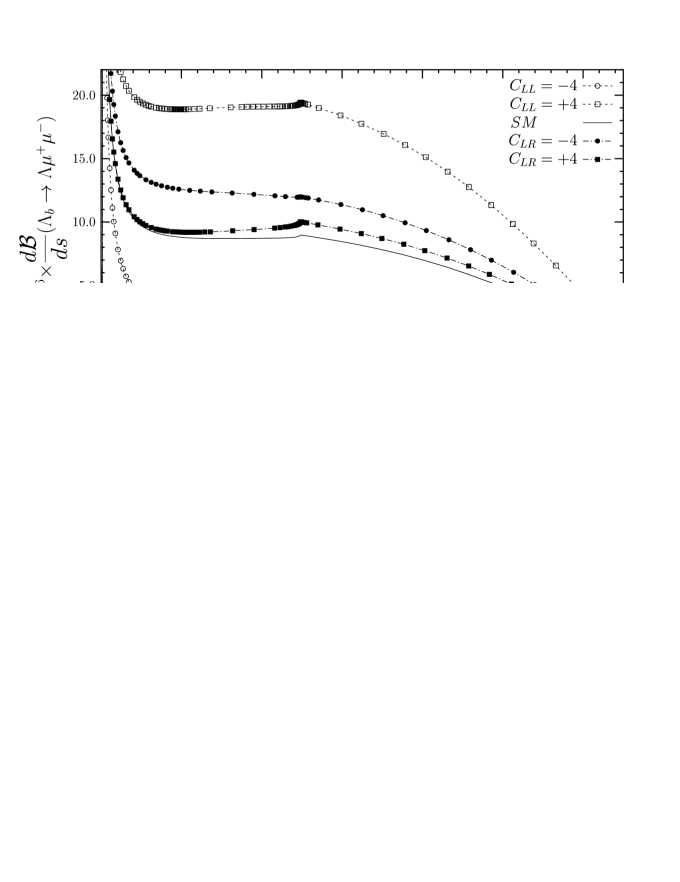
Figure 1:

Figure 2:

Figure 3:

Figure 4:

Figure 5:

Figure 6:

Figure 7:

Figure 8:

Figure 9:

Figure 10:

Figure 11:

Figure 12:

Figure 13:

Figure 14:

Figure 15:

Figure 16:

References

• [1] The BaBar Physics book, Eds: P. F. Harrison, H. R. Quinn, SLAC report, (1998) 504;
BELLE Collaboration, E. Drebys at. al, Nucl. Instrum. Methods A446 (2000) 89.
• [2] CLEO Collaboration, M. S. Alan at. al, Phys. Rev. Lett. 74 (1995) 2885.
• [3] W. S. Hou, R. S. Willey and A. Soni, Phys. Rev. Lett. 58, 1608 (1987).
• [4] N. G. Deshpande and J. Trampetic, Phys. Rev. Lett. 60, 2583 (1988).
• [5] C. S. Kim, T. Morozumi and A. I. Sanda, Phys. Lett. B218, 343 (1989).
• [6] B. Grinstein, M. J. Savage and M. B. Wise, Nucl. Phys. B319, 271 (1989).
• [7] C. Dominguez, N. Paver and Riazuddin, Phys. Lett. B214, 459 (1988).
• [8] N. G. Deshpande, J. Trampetic and K. Ponose, Phys. Rev. D39, 1461 (1989).
• [9] P. J. O’Donnell and H. K. Tung, Phys. Rev. D43, 2067 (1991).
• [10] N. Paver and Riazuddin, Phys. Rev. D45, 978 (1992).
• [11] A. Ali, T. Mannel and T. Morozumi, Phys. Lett. B273, 505 (1991).
• [12] A. Ali, G. F. Giudice and T. Mannel, Z. Phys. C67, 417 (1995).
• [13] C. Greub, A. Ioannissian and D. Wyler, Phys. Lett. B346, 145 (1995);
D. Liu, Phys. Lett. B346, 355 (1995);
G. Burdman, Phys. Rev. D52, 6400 (1995);
Y. Okada, Y. Shimizu and M. Tanaka, Phys.Lett. B405, 297 (1997).
• [14] A. J. Buras and M. MΓΌnz, Phys. Rev. D52, 186 (1995).
• [15] N. G. Deshpande, X. -G. He and J. Trampetic, Phys. Lett. B367, 362 (1996).
• [16] S. Bertolini, F. Borzumati, A. Masiero, G. Ridolfi,
Nucl.Phys. B353, 591 (1991).
• [17] F. KrΓΌger and L. M. Sehgal Phys. Rev. D55,2799 (1997).
• [18] F. KrΓΌger and L. M. Sehgal Phys. Rev. D56, 5452 (1997).
• [19] T. M. Aliev, A. Γ–zpineci, M. SavcΔ±, Phys. Rev. D56 (1997) 4260.
• [20] P. Ball, V. M. Braun, Phys. Rev. D58 (1998) 094016.
• [21] T. M. Aliev, C. S. Kim, Y. G. Kim, Phys. Rev. D62 (2000) 014026.
• [22] T. M. Aliev, D. A. Demir, M. SavcΔ±, Phys. Rev. D62 (2000) 074016.
• [23] Chuan–Hung Chen and C. Q. Geng, Phys. Rev. D63 (2001) 054005; Phys. Rev. D63 (2001) 114024; Phys. Rev. D64 (2001) 074001.
• [24] T. M. Aliev, M. SavcΔ±, J. Phys. G26 (2000) 997.
• [25] S. Fukae, C. S. Kim, T. Morozumi, T. Yoshikawa, Phys. Rev. D59 (1999) 074013.
• [26] S. Fukae, C. S. Kim, T. Yoshikawa, Phys. Rev. D61 (2000) 074015.
• [27] T. M. Aliev, A. Γ–zpineci, M. SavcΔ±, Phys. Lett. B511 (2001) 49; Phys. Lett. B506 (2001) 77; T. M. Aliev, M. K. Γ‡akmak, M. SavcΔ±, Nucl. Phys. B607 (2001) 305.
• [28] T. M. Aliev, A. Γ–zpineci, M. K. Γ‡akmak, M. SavcΔ±, Phys. Rev. D64 (2001) 055007.
• [29] T. Mannel, W. Roberts and Z. Ryzak, Nucl. Phys. B355 (1991) 38.
• [30] Chuan–Hung Chen and C. Q. Geng, Phys. Lett. B516 (2001) 327.
• [31] CDF Collaboration, T. Affolder at. al, Phys. Rev. Lett. 83 (1999) 3378; CLEO Collaboration, Yongsheng Gao, prep: hep–ex/0108005 (2001).