Abstract

An Effective String Rope Model (ESRM) for heavy ion collisions at RHIC energies is presented. Our model takes into account baryon recoil for both target and projectile, arising from the acceleration of partons in an effective field, produced in the collision. The typical field strength (string tension) for RHIC energies is about $5-12\ GeV/fm$, what allows us to talk about “string ropes”. Now we describe an ”expanding final streaks” scenario [7], in contrast to a ”non-expanding final streaks” discussed in Ref. [8]. The results show that a QGP forms a tilted disk, such that the direction of the largest pressure gradient stays in the reaction plane, but deviates from both the beam and the usual transverse flow directions. The produced initial state can be used as an initial condition for further hydrodynamical calculations. Such initial conditions lead to the creation of a third flow component.

The realistic and detailed description of an energetic heavy ion reaction requires a Multi Module Model, where the different stages of the reaction are each described with a suitable theoretical approach. It is important that these Modules are coupled to each other correctly: on the interface, which is a three dimensional hypersurface in space-time with normal $d\sigma^{\mu}$, all conservation laws should be satisfied, and entropy should not decrease. These matching conditions were worked out and studied for the matching at FO hypersurfaces in details in Refs. [1, 2].

In energetic collisions of large heavy ions, one-fluid dynamics is a valid and good description for the intermediate stages of the reaction. Here, interactions are strong and frequent, so that other models, (e.g. transport models, string models, etc., that assume binary collisions, with free propagation of constituents between collisions) have limited validity. On the other hand, the initial and final, Freeze Out (FO), stages of the reaction are outside the domain of applicability of the fluid dynamical model. For the highest energies achieved nowadays at RHIC, hydrodynamic calculations give a good description of the observed radial and elliptic flows [3, 4, 5, 6].

The initial stages for RHIC energies are the most problematic. Non of the theoretical models currently on the physics market can unambiguously describe the initial stages (see [7] for a discussion).

1 Expanding final streaks in ESRM

In Refs. [9, 10, 8] we assumed that the final result of the collision of two streaks, after stopping the string’s expansion and after its decay, is one streak of the length $\bigtriangleup l_{f}$ with homogeneous energy density distribution, $e_{f}$, moving like one object with rapidity $y_{f}$ ($e_{f}$ and $y_{f}$ can be easily found from conservation laws). The typical values of the string tension, $\sigma$, are of the order of $10\ GeV/fm$, and these may be treated as several parallel strings. We assumed that such a final state is due to string-string interactions and string decays, which we are not going to describe in our simple model. One of the simplest ways to quantitatively take into account string decays is presented in Ref. [11].

Now we would like to describe the scenario with expanding final streaks, which seems to be more realistic [7]. It is based on the solution for the one-dimensional expansion of the finite streak into the vacuum, which can be found [7] generalizing the description in [12].

The initial condition is

$$e(z,t_{0}) = \left\{\begin{array}[]{ll}0&~{}~{}-\infty<z<R_{-}~{},\\ e_{0}&,~{}~{}R_{-}\leq z\leq R_{+}\\ 0&,~{}~{}R_{+}<z<\infty~{},\end{array}\right.$$ (4)

$$v(z,t_{0}) = \left\{\begin{array}[]{ll}-1&,~{}~{}-\infty<z<R_{-}\\ \tanh y_{0}&,~{}~{}R_{-}\leq z\leq R_{+}\\ 1&,~{}~{}R_{+}<z<\infty~{},\end{array}\right.\ ,$$ (8)

where $R_{-}$, $R_{+}$ are the borders of the system.

For the forward-going rarefaction wave, $v>0$, generated on the right end of the initial streak, we infer that the head of this wave (the point where the rarefaction of matter starts, i.e., where the energy density $e$ starts to fall below $e_{0}$) travels with the velocity $(\tanh y_{0}-c_{0})/(1-c_{0}\tanh y_{0})$ to the left. On the other hand, the base of the rarefaction wave (the point where $e$ starts to acquire non-vanishing values) travels with light velocity $v=1$ to the right. The solution for a simple wave has a similarity form [12], i.e., the profile of the rarefaction wave does not change with time when plotted as a function of the similarity variable $\zeta_{\pm}\equiv\frac{z\mp-R_{\pm}}{t-t_{0}}$. Thus,

$$e(\zeta_{+})=e_{0}\cdot\left\{\begin{array}[]{ll}1&,~{}~{}-1\leq\zeta_{+}\leq\frac{\tanh y_{0}-c_{0}}{1-c_{0}\tanh y_{0}}\\ {\displaystyle\left[\frac{1+\tanh y_{0}}{1-\tanh y_{0}}~{}\frac{1-c_{0}}{1+c_{0}}~{}\frac{1-\zeta_{+}}{1+\zeta_{+}}\right]}^{(1+c_{0}^{2})/2c_{0}}&,~{}~{}\frac{\tanh y_{0}-c_{0}}{1-c_{0}\tanh y_{0}}<\zeta_{+}\leq 1~{}.\end{array}\right.$$ (9)

$$\tanh y(\zeta_{+})=\left\{\begin{array}[]{ll}\tanh y_{0}&,~{}~{}-1\leq\zeta_{+}\leq\frac{\tanh y_{0}-c_{0}}{1-c_{0}\tanh y_{0}}\\ {\displaystyle\frac{c_{0}+\zeta_{+}}{1+\zeta_{+}c_{0}}}&,~{}~{}\frac{\tanh y_{0}-c_{0}}{1-c_{0}\tanh y_{0}}<\zeta_{+}\leq 1~{}.\end{array}\right.$$ (10)

Similarly for the backward-going rarefaction wave, $v<0$, we get

$$e(\zeta_{-})=e_{0}\cdot\left\{\begin{array}[]{ll}1&,~{}~{}\frac{\tanh y_{0}+c_{0}}{1+c_{0}\tanh y_{0}}\leq\zeta_{-}\leq 1\\ {\displaystyle\left[\frac{1-\tanh y_{0}}{1+\tanh y_{0}}~{}\frac{1-c_{0}}{1+c_{0}}~{}\frac{1+\zeta_{-}}{1-\zeta_{-}}\right]}^{(1+c_{0}^{2})/2c_{0}}&,~{}~{}-1<\zeta_{-}\leq\frac{\tanh y_{0}+c_{0}}{1+c_{0}\tanh y_{0}}~{},\end{array}\right.$$ (11)

$$\tanh y(\zeta_{-})=\left\{\begin{array}[]{ll}\tanh y_{0}&,~{}~{}\frac{\tanh y_{0}+c_{0}}{1+c_{0}\tanh y_{0}}\leq\zeta_{-}\leq 1\\ {\displaystyle\frac{\zeta_{-}-c_{0}}{1-\zeta_{-}c_{0}}}&,~{}~{}-1<\zeta_{-}\leq\frac{\tanh y_{0}+c_{0}}{1+c_{0}\tanh y_{0}}~{}.\end{array}\right.$$ (12)

This simple analytical solution is valid as long as the two rarefaction waves did not overlap in the middle of the system. Further evolution becomes more complicated and doesn’t have a similarity form any more.

Thus, based on the solution presented above we can have a more advanced description of the final streaks. Let us assume that the homogeneous final streaks, with some $e_{f}$, $y_{f}$, are formed in the Center-of-Rapidity frame (CRF) when the larger of initial streaks reach the rapidity $y_{f}$. Up to this point the fluid cell trajectories are the same as those for non-expanding scenario [8], but after the homogeneous final streak is formed, it starts to expand according to the simple rarefaction wave solution, eqs. (9-12) [7]. Figure 1 (B) shows new trajectories of the streak ends (compare to (A) from Ref. [8]), and Figures 1 (C,D) present energy density and rapidity profile for this expanding streak.

Such an initial state with expanding streaks will also help to avoid the problem which may cause the development of numerical artifacts, namely a step-like in the beam direction initial energy density distribution (output of ESRM): it has a jump from $e_{f}=const$ inside the matter, to $0$ in the outside vacuum (of course, where there is also a jump of $e$ as a function of $x,y$, but it is much smoother and this is not the direction of the initial expansion). In order to avoid (or at least to suppress) this effect, it was proposed in Ref. [13] to smooth over initial energy density distribution, for example by a Gaussian shape. Our simple analytic solution smoothes out this jump in a natural way.

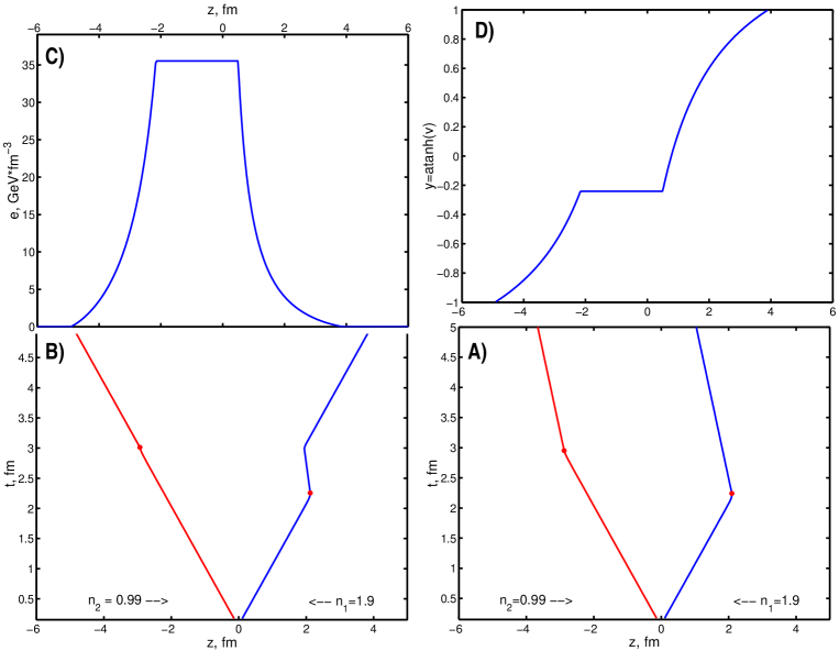
Figure 1: A) The typical trajectory of the ends of two initial streaks corresponding to the numbers of nucleons $n_{1}$ and $n_{2}$, $\varepsilon_{0}=65\ GeV/nucl$, $A=0.09$ (see ESRM description, for example [8]). Stars denote the points where $y_{1,2}=y_{f}$. From $t=t_{0}$ until these stars, the streak ends move according trajectories derived in Ref. [8] (see eqs. (37, 38)). Then the final streak starts to move like a single object with rapidity $y_{f}$ in CRF. B) The same situation as in subplot (A), but for expanding final streak. C) Shows $e(z)$ profiles of expanding final streak ($t_{h}=5\ fm$). We can clearly see three regions - two of forward and backward rarefaction waves and a middle where the initial energy density, $e_{f}$, is still preserved. D) Shows the rapidity profile of the expanding final streak ($t_{h}=5\ fm$). We can clearly see three regions - two of forward and backward rarefaction waves and a middle where the initial rapidity, $y_{f}$, is still preserved.

Fig. 2 shows the energy density distribution in the reaction plane for the RHIC collisions calculated in the scenario with expanding final streaks. The QGP forms a tilted disk for $b\not=0$. Thus, the direction of fastest expansion, the same as the largest pressure gradient, will be in the reaction plane, but will deviate from both the beam axis and the usual transverse flow direction. So, the new “third flow component” [14] appears in addition to the usual transverse flow component in the reaction plane. For non-expanding streaks this was shown in [15]. If we let final streaks expand, this smoothes out the picture, but most of the matter, nevertheless, keeps a similar energy density profile and velocity distribution.

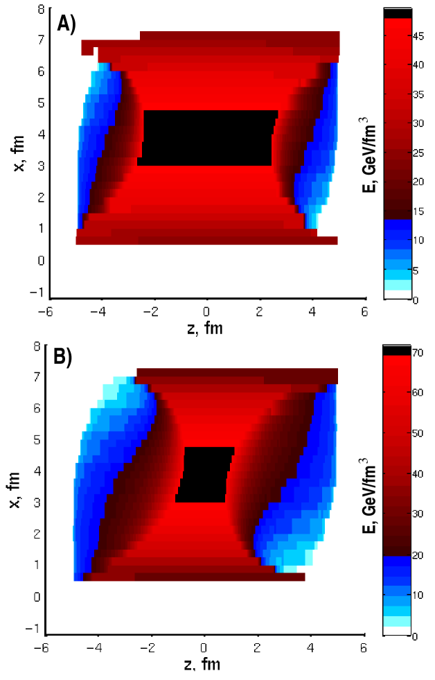
Figure 2: Au+Au collision at $\varepsilon_{0}=100\ GeV/nucl$, $\left(b=0.5\cdot 2\ R_{Au}\right)$ , $E=T^{00}$ is presented in the reaction plane as a function of $x$ and $z$ for $t_{h}=5\ fm/c$. Subplot A) $A=0.065$, subplot B) $A=0.08$. The QGP volume has a shape of a tilted disk and may produce a third flow component.

References

- [1] Cs. Anderlik et al, Phys. Rev. C 59 (1999) 388; Phys. Rev. C 59 (1999) 3309; Phys. Lett. B 459 (1999) 33.
- [2] V.K. Magas et al, Heavy Ion Phys. 9 (1999) 193, (nucl-th/9903045); Nucl. Phys. A 661 (1999) 596.
- [3] Josef Sollfrank et al, Phys. Rev C55, 392 (1997).
- [4] U. Ornik et al, Phys. Rev. C54 1381 (1996).
- [5] P. Huovinen et al, Phys. Lett B503, 58 (2001).
- [6] D. Teaney, J. Lauret, and E.V. Shuryak, Phys. Rev. Lett. 86, 4783 (2001).
- [7] V. Magas, L.P. Csernai, D. Strottman, hep-ph/0202085.
- [8] V. Magas, L.P. Csernai, D. Strottman, Phys. Rev. C 64 (2001) 014901.
- [9] V.K. Magas, L.P. Csernai, D.D. Strottman, nucl-th/0009049, hep-ph/0101125.
- [10] L.P. Csernai, Cs. Anderlik, V.K. Magas, nucl-th/0010023.
- [11] I.N. Mishustin, J.I. Kapusta, hep-ph/0110321.
- [12] D. Rischke, S. Bernard, J.A. Maruhn, Nucl. Phys. A 595 (1995) 346.
- [13] T. Hirano, nucl-th/0108004.
- [14] L.P. Csernai, D. Röhrich, Phys. Lett. B 458 (1999) 454.
- [15] V.K. Magas, L.P. Csernai and D. Strottman, hep-ph/0110347.