Asymmetric Chern-Simons number diffusion from CP-violation

Abstract

We study Chern-Simons number diffusion in a SU($2$)-Higgs model with CP-odd dimension-eight operators. We find that the thermal average of the magnitude of the velocity of the Chern-Simons number depends on the direction of the velocity. This implies that the distribution function of the Chern-Simons number will develop an asymmetry. It is argued that this asymmetry manifests itself through a linear growth of the expectation value of the third power of the Chern-Simons number. This linear behavior of the third power of a coordinate of a periodic direction is verified by a numerical solution of a one-dimensional Langevin equation. Further, we make some general remarks on thermal averages and on the possibility of the generation of the baryon asymmetry in a non-equilibrium situation due to asymmetric diffusion of the Chern-Simons number.

1 Introduction

An important cosmological observation is the matter-antimatter asymmetry in the present universe. This asymmetry may be quantified by the baryon-to-photon ratio, whose observational value is [1]

$$\frac{n_{B}}{n_{\gamma}}=(1.55-4.45)\times 10^{-10},$$ (1)

with $n_{B}$ the baryon number density and $n_{\gamma}$ the photon density. An interesting question is how this asymmetry was generated in the early universe. In his 1967 paper Sakharov [2] notes that baryon number can only be generated when
1) baryon number is not conserved,
2) the transformations C and CP are not symmetries,
3) there is a departure from equilibrium.

In 1976 ’t Hooft [3] showed that in the electroweak theory the first requirement is satisfied. The non-trivial vacuum structure of the SU($2$)-gauge theory in combination with the anomaly equation implies that a change in Chern-Simons number, $N_{\rm CS}$, is accompanied by a change in baryon number, $B$,

$$B(t)-B(0) = 3\left[N_{\rm CS}(t)-N_{\rm CS}(0)\right]$$ (2)

$$= \frac{3g^{2}}{32\pi^{2}}\int_{0}^{t}dt^{\prime}\int d^{3}xF_{\mu\nu}^{a}\tilde{F}^{\mu\nu a},$$

with $g$ the SU($2$)-gauge-coupling, $F_{\mu\nu}^{a}$ the field strength, and $\tilde{F}^{\mu\nu a}$ its dual. At zero temperature changes in the Chern-Simons number involve instanton processes. The rate of these processes is very small [3]. However, at high temperature the rate is much larger. As has long been recognized this opens up the possibility that the baryon asymmetry was generated at temperatures of about $100$ GeV [4], when the (elementary) particles that made up the plasma may be described by the electroweak theory.

However, within the standard model the amount of CP-violation is probably too small to account for the observed asymmetry (1) [5]. One way to deal with this is to include effective non-renormalizable operators that parameterize the CP-violation of a more fundamental theory. The lowest-dimensional operator in a SU($2$)-Higgs theory is $\phi^{\dagger}\phi F_{\mu\nu}^{a}\tilde{F}^{\mu\nu a}$, with $\phi$ the Higgs field. It may be included in the effective action as

$$S^{[6]}=\frac{3g^{2}\delta_{\rm CP}^{0}}{32\pi^{2}M^{2}}\int d^{4}x\phi^{\dagger}\phi F_{\mu\nu}^{a}\tilde{F}^{\mu\nu a},$$ (3)

with $M$ a mass and $\delta_{\rm CP}^{0}$ a coefficient that ideally may be derived from the fundamental theory. In the current investigation dimension-eight operators will play a more important role. They may be included in the action as

$$S^{[8]}=\frac{3g^{2}}{32\pi^{2}M^{4}}\int d^{4}x\left[\delta_{\rm CP}^{1}(D_{\rho}\phi)^{\dagger}(D^{\rho}\phi)-\delta_{\rm CP}^{2}F_{\rho\sigma}^{b}F^{\rho\sigma b}+\delta_{\rm CP}^{3}(\phi^{\dagger}\phi)^{2}\right]F_{\mu\nu}^{a}\tilde{F}^{\mu\nu a},$$ (4)

with $D_{\rho}$ the covariant derivative.

In this paper we study the combination of the first two of Sakharov’s requirements, although we were unable to refrain from making some remarks on the inclusion of the third one in our study. That is, we study the motion of the Chern-Simons number in the SU($2$)-Higgs action extended with (3) and (4). It is well known that in a pure SU($2$)-Higgs theory (without extra CP-odd operators and without fermions) the long-time behavior of the Chern-Simons number may be viewed as a diffusion process in one dimension, that can be specified by the expectation values

$$\langle N_{\rm CS}(t)-N_{\rm CS}(0)\rangle = 0,$$ (5)

$$\langle\left[N_{\rm CS}(t)-N_{\rm CS}(0)\right]^{2}\rangle = 2V\Gamma_{\rm sph}t,$$ (6)

with $V$ the volume and $\Gamma_{\rm sph}$ the sphaleron rate. The sphaleron rate plays an important role in scenarios for electroweak baryogenesis, since it determines the rate of the baryon-number violating processes. Much effort has gone into the determination of the sphaleron rate, both in the symmetric phase [6],[7],[8] as well as in the broken phase [9],[10],[11]. Here, only the broken-phase sphaleron-rate will be needed

$$\Gamma_{\rm sph}=\kappa T^{4}e^{-\beta E_{\rm sph}},$$ (7)

with the sphaleron energy $E_{\rm sph}$, and $\kappa$ a dimensionless coefficient that depends on the temperature, the Higgs mass and expectation value, and the gauge coupling. The physical picture that underlies (7) is that of classical transitions from one (classical) vacuum to the next over a potential barrier of height $E_{\rm sph}$. On the basis of this picture, the gauge-Higgs dynamics will be treated classically in this paper.

The idea that the inclusion of CP-violating operators may have an interesting effect on the diffusion of the Chern-Simons number stems from the fact that the Chern-Simons number itself is CP-odd. Therefore the motion over the barrier towards positive Chern-Simons numbers may differ from the motion in the direction of negative Chern-Simons numbers. It is clear then, that the distribution function of the Chern-Simons number does not need to develop symmetrically. Or put differently: there is no symmetry argument why expectation values of odd powers of $N_{\rm CS}(t)-N_{\rm CS}(0)$ should vanish. In fact, we will show that an asymmetry in the distribution function will develop indeed (as may have been inferred from the title). That is, an initially symmetric distribution function will develop an asymmetry. In the presence of the CP-odd operators in (4) an equation for the expectation value of the third power of $N_{\rm CS}(t)-N_{\rm CS}(0)$ needs to be added to equations (5) and (6) to characterize the diffusion. We will argue that this expectation value increases linearly in time in the broken phase:

$$\langle\left[N_{\rm CS}(t)-N_{\rm CS}(0)\right]^{3}\rangle\sim t,$$ (8)

A more detailed conjecture is given in equation (56).

We end the introduction with a short outline of the rest of the paper. In the next section the dynamics of the gauge-Higgs system will be projected on a one-dimensional path through the configuration space. This will simplify the analysis of the rest of the paper. In section 3 we will calculate the thermal average of the velocity when the system moves in the direction of positive or negative Chern-Simons numbers. In section 4 a conjecture for the time dependence of $\langle[N_{\rm CS}(t)-N_{\rm CS}(0)]^{3}\rangle$ is presented, where it is argued to grow linearly in time. This linear growth is also present in a simple random walk model as is shown in appendix B. Section 5 contains some general remarks on statistical averages. In the following section, we derive a simple stochastic equation that is useful to verify some of the analytic results. Also some numerical solutions are presented. In section 7 we discuss how asymmetric diffusion of the Chern-Simons number may yield a non-zero baryon number in a out-of-equilibrium situation. Also some comments are made on the constraints on such a model. We end with a summary in section 8.

2 Projection of the dynamics of the gauge and Higgs fields onto one special direction in configuration space

To simplify the later study of the effect of the CP-violating operators in (3) and (4) on the diffusion of the Chern-Simons number, the gauge-Higgs-field dynamics is projected on a single path through the configuration space. In order to include sphaleron transitions, we use a path that runs from a classical vacuum to the sphaleron configuration and further to the next vacuum. Manton [12] defined such a path in his proof that a non-contractible loop exists in configuration space of the SU($2$)-Higgs model. This is the path that will be used in the following. The path of Manton is not the minimal-energy path, which was constructed in [13]. But the precise path will not be important for the following rather general arguments and we expect that the results will suffice as order of magnitude estimates.

We parameterize the path of Manton by the time-dependent coordinate $\Theta$. The fields are given in the radial gauge ($\partial_{i}A^{ia}=0$) by

gauge $$A_{\mu}^{a}\sigma^{a}=\frac{-2i}{g}f(\rho)[\partial_{\mu}U(\Theta)]U^{-1}(\Theta),$$ (9)

Higgs $$\phi=\frac{1}{2}\sqrt{2}v\left\{h(\rho)U(\Theta)\left(\begin{array}[]{c}0\\ 1\end{array}\right)-i[1-h(\rho)]\cos\Theta\left(\begin{array}[]{c}0\\ 1\end{array}\right)\right\},$$ (14)

with $v$ the Higgs expectation value and $\rho=gvr$, where $r=|\vec{x}|$. The $\Theta$-dependent SU($2$)-matrix is given by

$$U(\Theta)=\frac{1}{r}\left(\begin{array}[]{cc}z&x+iy\\ -x+iy&z\end{array}\right)\sin\Theta+\left(\begin{array}[]{cc}i&0\\ 0&-i\end{array}\right)\cos\Theta.$$ (15)

The functions $f$ and $h$ satisfy the boundary conditions

$$f\rightarrow 0 h\rightarrow 0\;\;\;\;\;\;\;r\rightarrow 0,$$

$$f\rightarrow 1 h\rightarrow 1\;\;\;\;\;\;\;r\rightarrow\infty.$$ (16)

The form of the fields (9), (14) is a non-static generalization of the fields considered in [12]. When $\Theta$ is chosen to be time-independent the fields given by (9), (14) can be identified (up to a global U($1$) gauge transformation) with the fields ($3.17$) in [12] (the coordinate $\Theta$ corresponds to $\mu$ in [12]).

For the functions $f$ and $h$ the Ansatz b of Klinkhamer and Manton [14] will be used

$$f(\rho) = \left\{\begin{array}[]{llr}\frac{\rho^{2}}{A(A+4)}&\rho\leq A\\ 1-\frac{4}{A+4}\exp[\frac{1}{2}(A-\rho)]&\rho\geq A\end{array}\right.,$$ (19)

$$h(\rho) = \left\{\begin{array}[]{llr}\frac{\sigma B+1}{B(\sigma B+2)}\rho&\rho\leq B\\ 1-\frac{B}{\sigma B+2}\frac{1}{\rho}\exp[\frac{1}{2}(B-\rho)]&\rho\geq B\end{array}\right.,$$ (22)

with $\sigma=(\lambda/2g^{2})^{{\scriptstyle\frac{1}{2}}}$, where $\lambda$ is the Higgs self-coupling constant. The parameters $A,B$ were determined by minimizing the energy for the static field configuration at $\Theta=\pi/2$ in [14], in order to obtain an estimate for the sphaleron energy. In this way the parameters depend only on $\sigma$. We take $\sigma=1$, for which the parameters have the values $A=1.15$ and $B=1.25$ [14].

Now that the dynamics has been restricted to the path described by (9) and (14) we may rewrite the SU($2$)-Higgs action, $S$, in terms of the coordinate $\Theta$

$$S[\dot{\Theta},\Theta]=\frac{4\pi v}{g}\int dt\left[\left(a_{1}+a_{2}\sin^{2}\Theta\right)\frac{\dot{\Theta}^{2}}{(gv)^{2}}-\left(a_{3}\sin^{2}\Theta+a_{4}\sin^{4}\Theta\right)\right].$$ (23)

The CP-odd action (4) in terms of $\Theta$ reads

$$S^{[8]}[\dot{\Theta},\Theta]=\frac{4\pi v^{2}}{M^{4}}\int dt\left[b_{1}\delta_{\rm CP}^{1}+b_{2}\delta_{\rm CP}^{2}+(b_{3}\delta^{1}_{\rm CP}+b_{4}\delta^{2}_{\rm CP})\sin^{2}\Theta\right]\dot{\Theta}^{3}\sin^{2}\Theta,$$ (24)

where total time-derivatives have been neglected.

The action $S^{[6]}$ (3), that includes the dimension-six operator $\phi^{\dagger}\phi F\tilde{F}$, gives only a total time-derivative, just as the operator $(\phi^{\dagger}\phi)^{2}F_{\mu\nu}^{a}\tilde{F}^{\mu\nu a}$ in (4). Therefore the inclusion of $S^{[6]}$ will not affect the motion along the path parameterized above. When the full field-dynamics is considered, the dimension-six operator may have an effect on the motion along the Chern-Simons number direction in a non-equilibrium situation, see e.g. [15]. In equilibrium however, the system oscillates around one vacuum or, during a transition, around the minimal-energy path that connects two classical vacua (the path that we have approximated by (9) and (14)). Since, the oscillations average out in equilibrium, we do not expect the inclusion of $S^{[6]}$ to affect the diffusion of the Chern-Simons number.

The coefficients $a_{1}$, $a_{2}$, $a_{3}$, $a_{4}$, $b_{1}$, $b_{2}$, $b_{3}$ $b_{4}$ are given by the integrals

$$a_{1} = \int_{0}^{\infty}d\rho\,\rho^{2}\left[(\partial_{\rho}f)^{2}+\frac{1}{2}(h-f)^{2}\right]=2.03,$$ (25)

$$a_{2} = \int_{0}^{\infty}d\rho\,\left[8f^{2}(1-f)^{2}+\frac{1}{2}(1-h^{2})(1-f^{2})\rho^{2}\right]=2.53,$$ (26)

$$a_{3} = \int_{0}^{\infty}d\rho\left[4(\partial_{\rho}f)^{2}+\frac{1}{2}\rho^{2}(\partial_{\rho}h)^{2}+h^{2}(1-f)^{2}\right.$$ (27)

$$\hskip 28.45274pt\left.-2fh(1-f)(1-h)+f^{2}(1-h)^{2}\right]=1.41,$$

$$a_{4} = \int_{0}^{\infty}d\rho\left[8f^{2}(1-f)^{2}/\rho^{2}+2fh(1-f)(1-h)\phantom{\frac{1}{4}}\right.$$ (28)

$$\hskip 28.45274pt\left.-f^{2}(1-h)^{2}+\frac{1}{4}\rho^{2}(1-h^{2})^{2}\right]=0.70,$$

$$b_{1} = \frac{9}{2}\int_{0}^{\infty}d\rho\,(h-f)^{2}(\partial_{\rho}f)f(1-f)=0.09,$$ (29)

$$b_{2} = 9\int_{0}^{\infty}d\rho(\partial_{\rho}f)^{3}f(1-f)=0.10,$$ (30)

$$b_{3} = \frac{9}{2}\int_{0}^{\infty}d\rho(1-h^{2})(\partial_{\rho}f)f(1-f)(1-f^{2})=0.19,$$ (31)

$$b_{4} = 72\int_{0}^{\infty}d\rho\frac{1}{\rho^{2}}(\partial_{\rho}f)f^{3}(1-f)^{3}=0.16.$$ (32)

Let us shortly discuss the actions (23) and (24). In the action (23) we recognize the potential barrier [12],

$$V(\Theta)=\frac{4\pi v}{g}\left[a_{3}\sin^{2}\Theta+a_{4}\sin^{4}\Theta\right],$$ (33)

between different vacua. The sphaleron energy reads

$$E_{\rm sph}=V(\Theta=\frac{1}{2}\pi)=(a_{3}+a_{4})\frac{4\pi v}{g}=2.11\frac{4\pi v}{g}.$$ (34)

The sphaleron energy determines the exponential suppression of the sphaleron rate (7). Another quantity that enters the sphaleron rate is (the real part of) the frequency of the negative mode, $\omega_{-}$, at the sphaleron configuration [9]. From the action (23) it may be determined as

$$\omega_{-}^{2}=\frac{a_{3}+2a_{4}}{a_{1}+a_{2}}(gv)^{2}\approx 0.61(gv)^{2}.$$ (35)

In agreement with the order of magnitude estimate $\omega_{-}\sim gv$ in [9].

The action (24) is odd in $\Theta$. This can be understood by realizing that a CP-transformation in terms of $\Theta$ is

$$\Theta\rightarrow-\Theta,$$ (36)

since the action (4) is CP-odd, so should (24).

Now that the SU($2$)-Higgs action including the effective CP-odd operators has been immensely simplified, namely to the one-dimensional action (23) $+$ (24), the question: ”does the Chern-Simons number diffuse asymmetrically under the influence of the dimension-eight operators in the action (4)?” may be cast in the form: ”does the factor $\dot{\Theta}^{3}$ in (24) lead to an asymmetric diffusion of $\Theta$?”. What is meant by ”diffusion of $\Theta$” may require some explanation. From equations (9),(14), and (15), one sees that $\Theta=0$ and $\Theta=2\pi$ correspond to the same (static) gauge and Higgs field configuration. Even $\Theta=0$ and $\Theta=\pi$ correspond to the same physical state, since they are related by a simple gauge transformation. Hence, one may view configuration space as a circle with circumference $\pi$.

This is the same for the full gauge-Higgs fields. When a transition over the sphaleron barrier is considered, the system starts and ends in the same state (since the different vacua are related by a large gauge transformation). Nevertheless the winding number is changed: $\Delta N_{\rm CS}=1$. The (change in the) winding number is the physical quantity of interest, since it is related to the (change in the) baryon number through (2). The relation between a change in the Chern-Simons number and $\Theta$ is (see Appendix A)

$$N_{\rm CS}(t)-N_{\rm CS}(0)=\frac{2}{\pi}\int_{0}^{t}dt^{\prime}\dot{\Theta}\sin^{2}\Theta.$$ (37)

Instead of considering the system on a circle and keeping track of the winding number, it is convenient to ”unwind” the system and consider the system on an infinite line $\Theta\in]-\infty,\infty[$ and follow the dynamics of $\Theta$ (see figure 1). Thus, we consider the diffusion of $\Theta\in]-\infty,\infty[$, where we keep in mind that actually we consider the winding number on a circle.

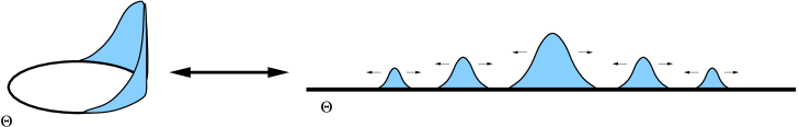
Figure 1: The distribution function of $\Theta$ in a periodic potential. On the left it is viewed on the circle $\Theta\in[0,\pi[$, then the distribution function is static. On the right it is unwound to the infinite line $\Theta\in]-\infty,\infty[$ accounting thus for the winding number naturally. On the infinite line the system is dynamical and the distribution function diffuses.

To discuss the diffusion of $\Theta$ in the next section it is convenient to derive the Hamiltonian. Firstly, we write the Langrangian corresponding to (23) and (24) as

$$L=z_{1}(\Theta)\dot{\Theta}^{2}+z_{2}(\Theta)\dot{\Theta}^{3}-V(\Theta),$$ (38)

with

$$z_{1}(\Theta) = \frac{4\pi}{g^{3}v}(a_{1}+a_{2}\sin^{2}\Theta),$$ (39)

$$z_{2}(\Theta) = \frac{4\pi v^{2}}{M^{4}}[b_{1}\delta^{1}_{\rm CP}+b_{2}\delta^{2}_{\rm CP}+(b_{3}\delta^{1}_{\rm CP}+b_{4}\delta^{2}_{\rm CP})\sin^{2}\Theta]\sin^{2}\Theta.$$ (40)

Clearly the kinetic energy in (38) is unbounded. And, for instance, a (CP-even) $\dot{\Theta}^{4}$ is required to put a lower bound on the kinetic energy. Such a $\dot{\Theta}^{4}$ term should come from a higher (non-renormalizable) operator, so it is expected to be suppressed compared to the other CP-even $\dot{\Theta}^{2}$-term. Therefore the details of the $\dot{\Theta}^{4}$-term are unimportant for the following calculations. In fact strictly to first order in $\delta_{\rm CP}^{1}$ and $\delta_{\rm CP}^{2}$ (which are assumed to be small), one can work with the unbounded Lagrangian (38) (and the unbounded Hamiltonian (42)), although it may be kept in mind that a $\dot{\Theta}^{4}$-term (or higher even powers of $\dot{\Theta}$) are required for a bounded energy. We assume that these higher-order CP-even terms will make the Lagrangian convex, so that we can go to a Hamiltonian description. The conjugate momentum then reads

$$p=2z_{1}(\Theta)\dot{\Theta}+3z_{2}(\Theta)\dot{\Theta}^{2},$$ (41)

and the Hamiltonian

$$H(p,\Theta)=\frac{1}{4z_{1}(\Theta)}p^{2}-\frac{z_{2}(\Theta)}{8[z_{1}(\Theta)]^{3}}p^{3}+V(\Theta).$$ (42)

This is the Hamiltonian that will be used for the calculation of statistical averages in the next section.

The point of this section was to show that the CP-odd operators in $S^{[8]}$ (4) projected onto the one-dimensional path in phase space gives a $p^{3}$-term in the Hamiltonian and a $\dot{\Theta}^{3}$-term in the Lagrangian, and to give reasonable estimates for the coefficients in the projected action and Hamiltonian. The main subject of this paper, the effect of the CP-odd terms on the dynamics, will be discussed in the next and following sections.

3 Velocity expectation values

We study the effect of the action (4) on the diffusion of the Chern-Simons number. For this the Hamiltonian (42) will be used. We will work to first order in the coefficients $\delta_{\rm CP}^{1}$ and $\delta_{\rm CP}^{2}$ (and hence, to first order in $z_{2}$). So the question is what does the diffusion of $\Theta$ look like to first order in $\delta_{\rm CP}^{1}$ and $\delta_{\rm CP}^{2}$. In particular, will the distribution function of $\Theta$ develop an asymmetry?

The first thing one may notice is that (the magnitude of) the velocity differs for positive or negative $\dot{\Theta}$. More precisely, at a given momentum ($p$) or at a given energy ($H$) the magnitude of the velocity depends on its direction. This implies that the motion over the barrier towards negative Chern-Simons number differs from the motion towards positive Chern-Simons number. Hence, an asymmetry is expected to develop.

It is useful to define a quantity that ”measures” the asymmetry. A simple and useful quantity is the mean velocity, at a certain position, when $\Theta$ moves either to the right or to the left. We define

$$v^{\uparrow}(\bar{\Theta}) = \langle|\dot{\Theta}|{\cal H}(\dot{\Theta})\delta(\Theta-\bar{\Theta})\rangle/\langle{\cal H}(\dot{\Theta})\delta(\Theta-\bar{\Theta})\rangle,$$ (43)

$$v^{\downarrow}(\bar{\Theta}) = \langle|\dot{\Theta}|{\cal H}(-\dot{\Theta})\delta(\Theta-\bar{\Theta})\rangle/\langle{\cal H}(-\dot{\Theta})\delta(\Theta-\bar{\Theta})\rangle,$$ (44)

where the brackets denote a thermal average, and ${\cal H}$ the Heaviside function. When the difference

$$\Delta v(\bar{\Theta})=v^{\uparrow}(\bar{\Theta})-v^{\downarrow}(\bar{\Theta})$$ (45)

is non-zero, an asymmetry will develop. Consider, for instance, the evolution of the distribution function of $\Theta$. When the particles that move to the left do it faster (slower) than the particles that move to the right, the tail of the distribution function to the left extends more (less) than to the right. Hence, the distribution function develops an asymmetry. In particular, we expect expectation values of odd powers of $\Theta$ to become negative (positive) when the distribution function is initially symmetric and thermal.

In the calculation of the velocities (43) and (44), firstly one may remark that their numerators are equal. This follows from the fact that the flux through a point

$$\langle\dot{\Theta}\delta(\Theta-\bar{\Theta})\rangle=\langle|\dot{\Theta}|{\cal H}(\dot{\Theta})\delta(\Theta-\bar{\Theta})\rangle-\langle|\dot{\Theta}|{\cal H}(-\dot{\Theta})\delta(\Theta-\bar{\Theta})\rangle$$ (46)

vanishes. This may be seen from

$$\langle\dot{\Theta}\delta(\Theta-\bar{\Theta})\rangle = \langle\partial_{p}H\delta(\Theta-\bar{\Theta})\rangle$$ (47)

$$= Z_{\pi}^{-1}\int_{\-\infty}^{\infty}dp\int_{-\pi/2}^{\pi/2}d\Theta\partial_{p}H\delta(\Theta-\bar{\Theta})e^{-\beta H}$$

$$= -Z_{\pi}^{-1}T\int_{\-\infty}^{\infty}dp\int_{-\pi/2}^{\pi/2}d\Theta\delta(\Theta-\bar{\Theta})\partial_{p}e^{-\beta H}=0.$$

Here we used that $\exp-\beta H$ vanishes at $p=\pm\infty$, for which we had to keep in mind that a $p^{4}$-term in the Hamiltonian is required to make it bounded and convex. (Alternatively, strictly working to first order in $\delta_{\rm CP}^{1}$ and $\delta_{\rm CP}^{2}$, the momentum integrations in (47) also vanish.) The normalization factor $Z_{\pi}$ is defined as usual, see (59). It will drop out of the calculation of the velocities $v^{\uparrow}$ and $v^{\downarrow}$. The fact that the flux vanishes, implies that the expectation value of $\Theta$ remains constant:

$$\langle\Theta(t)-\Theta(0)\rangle=0,$$ (48)

as will be discussed more fully in the section 5. Hence, asymmetric diffusion will affect only expectation values of higher odd powers of $\Theta$.

The result for the numerator on the r.h.s. of (43) (equal to the numerator on the r.h.s. of (44)) is

$$\langle|\dot{\Theta}|{\cal H}(\dot{\Theta})\delta(\Theta-\bar{\Theta})\rangle = Z_{\pi}^{-1}\int_{-\infty}^{\infty}dp\int_{-\pi/2}^{\pi/2}d\Theta\partial_{p}H{\cal H}(p)\delta(\Theta-\bar{\Theta})e^{-\beta H}$$ (49)

$$= Z_{\pi}^{-1}Te^{-\beta V(\bar{\Theta})}.$$

The denominator of (43) is given by

$$\langle{\cal H}(\dot{\Theta})\delta(\Theta-\bar{\Theta})\rangle = Z_{\pi}^{-1}e^{-\beta V(\bar{\Theta})}\int_{0}^{\infty}dp\,e^{-\beta\frac{1}{4z_{1}(\bar{\Theta})}p^{2}+\beta\frac{z_{2}(\bar{\Theta})}{8[z_{1}(\bar{\Theta})]^{3}}p^{3}}$$ (50)

$$= Z_{\pi}^{-1}\left[\sqrt{\pi z_{1}(\bar{\Theta})T}+T\frac{z_{2}(\bar{\Theta})}{z_{1}(\bar{\Theta})}\right]e^{-\beta V(\bar{\Theta})},$$

to first order in $z_{2}$. The denominator of (44) yields

$$\langle{\cal H}(-\dot{\Theta})\delta(\Theta-\bar{\Theta})\rangle=Z_{\pi}^{-1}\left[\sqrt{\pi z_{1}(\bar{\Theta})T}-T\frac{z_{2}(\bar{\Theta})}{z_{1}(\bar{\Theta})}\right]e^{-\beta V(\bar{\Theta})}.$$ (51)

Hence, up to first order in $\delta_{\rm CP}^{1}$ and $\delta_{\rm CP}^{2}$ we have

$$v^{\uparrow(\downarrow)}(\bar{\Theta})=\sqrt{\frac{T}{\pi z_{1}(\bar{\Theta})}}-(+)\frac{T}{\pi[z_{1}(\bar{\Theta})]^{2}}z_{2}(\bar{\Theta}),$$ (52)

and

$$\Delta v(\bar{\Theta})=-\frac{2T}{\pi[z_{1}(\bar{\Theta})]^{2}}z_{2}(\bar{\Theta}),$$ (53)

The relative velocity difference,

$$\Delta v_{\rm rel}(\bar{\Theta}) = \frac{\Delta v(\bar{\Theta})}{v^{\uparrow}(\bar{\Theta})+v^{\downarrow}(\bar{\Theta})}$$ (54)

$$= -\sqrt{\frac{T}{\pi}}\frac{z_{2}(\bar{\Theta})}{[z_{1}(\bar{\Theta})]^{3/2}},$$

gives a (dimensionless) measure for the effect of CP-violation on diffusion.

In conclusion, we have established that, when $\Theta\not=0$, the magnitude of the thermal expectation value of the velocity depends on the direction in which $\Theta$ moves.

Let us consider what the difference in thermal expectations values of the velocity implies for the evolution of the distribution function of $\Theta$ and $p$, $P(p,\Theta,t)$. When the momentum, $p$, is thermally distributed independent of the position $\Theta$, the velocity difference is present in the entire ($\Theta$-)space. Now it is not hard to imagine that, when the particles move faster to the left than to the right, the tail of an initially symmetric thermal distribution function will (start to) extend more to the left than to the right. Therefore, a symmetric thermal distribution function will not remain symmetric. The diffusion develops asymmetrically when CP-odd terms like $\dot{\Theta}^{3}$ are included in the lagrangian. When we translate this result back to the gauge-Higgs system it implies that the inclusion of the CP-odd operators in (4) leads to an asymmetric diffusion of the Chern-Simons number.

4 Asymmetric diffusion: a conjecture for large times

In the previous section, it was shown that there is an asymmetry in the average velocity (54), which implies that the distribution function will develop an asymmetry. Hence, for instance, the expectation value of the third power of the Chern-Simons number, $\langle[N_{\rm CS}(t)-N_{\rm CS}(0)]^{3}\rangle$, will be nonzero. In this section, we will argue that this expectation value will grow linearly in time in the broken phase of the SU($2$)-Higgs model.

We assume that after a transition over the sphaleron barrier the system thermalizes before a following transition. This implies that the transitions are uncorrelated. This assumption is reasonable when the height of the barrier, $E_{\rm sph}$, is large compared to the temperature, $T$, and the motion over the barrier is damped sufficiently. (In our description in terms of $\Theta$, this would require $\Theta$ to be not-too-weakly coupled to the other modes in the plasma.)

On the basis of this assumption we can establish the time-dependence of the third power of the Chern-Simons number. We have established in the previous section that an asymmetry will develop in the distribution function starting from an symmetric thermal initial distribution function. Hence, after a time $\Delta t$ the expectation value $\langle[N_{\rm CS}(\Delta t)-N_{\rm CS}(0)]^{3}\rangle$ has a nonzero value. During the time $\Delta t$ the distribution function has spread over different vacua. Since we assume that the distribution is thermal in each vacuum, during the time from $\Delta t$ to $2\Delta t$, from each vacuum the distribution will diffuse asymmetrically in the same way as it did in the time interval from time $0$ to time $\Delta t$. The thermalization in each vacuum implies that in each time interval $\Delta t$, from each vacuum the same diffusion process takes place (relative to that vacuum). From this argument follows the result that the expectation value of the third power of the Chern-Simons number in the presence of CP-odd dimension-eight operators in the broken phase of the SU($2$)-Higgs model grows linearly in time. That the repetition of the same asymmetry in the diffusion process in each time interval leads to a linear growth, may be seen, for instance, from a random walk model, as is shown in Appendix B.

In section 5.1, we show that in general (without the above asumption) the expectation value of a third power of a coordinate $x$, $\langle x^{3}\rangle$, either stays constant or grows linearly in time in thermal equilibrium. A stochastic model that will be introduced later, shows that, with potential barriers, $\langle x^{3}\rangle$ grows linearly in time, and that without barriers $\langle x^{3}\rangle$ goes to a constant. This supports the view that barriers are required to ensure that the asymmetry in the diffusion process is independent of the position (which vacuum the system is in) and time, from which the linear behavior follows. In the symmetric phase, different vacua are not well separated by a barrier, therefore it is for us not possible to determine the time-dependence of asymmetric Chern-Simons number diffusion.

To obtain a more detailed conjecture for diffusion in the broken phase, we extend our one-dimensional model by coupling $\Theta$ to the other modes (that form the heat bath at temperature $T$) as in the full SU($2$)-Higgs model. In this way the rate for transitions over the barrier is given by $(gv)^{-3}\Gamma_{\rm sph}$, with $(gv)^{-3}$ the volume of the sphaleron. Then, we expect

$$\langle\Theta^{3}(t)\rangle\sim(gv)^{-3}\Gamma_{\rm sph}t\Delta v_{\rm rel,sph},$$ (55)

with the relative velocity difference (52) at the sphaleron configuration $\Delta v_{\rm rel,sph}=\Delta v_{\rm rel}(\pi/2)$.

By viewing the entire space as made up of blocks of volume ($gv)^{-3}$ in each of which a $\Theta$-coordinate is diffusing, one can translate (55) into an expectation value for the third power of the Chern-Simons number

$$\langle\left[N_{\rm CS}(t)-N_{\rm CS}(0)\right]^{3}\rangle=cV\Gamma_{\rm sph}t\Delta v_{\rm rel,sph},$$ (56)

with $V$ the volume and $c$ a constant of order one. In going from (55) to (56) we have in a very non-sophisticated manner included the zero mode for translation invariance. (It is conventional to include rotational zero modes in $\Gamma_{\rm sph}$ and exclude the translational zero modes.) A better way would have been to include the zero modes in the parameterization (9) and (14). However our aim is to investigate the occurrence of asymmetries for which the zero modes play no essential role.

5 Remarks on statistical averages

The Chern-Simons number diffusion is a non-equilibrium process. Still we, as many others, see e.g. [9], use a thermal (equilibrium) average to calculate the mean or average velocity of the Chern-Simons number (of $\Theta$ actually). In this subsection, we will briefly consider the use of statistical averages. In the next subsection, we return to dynamical issues and consider the possible time-dependence that an expectation value can have.

Consider a particle in one dimension coupled to a heat bath. In general one expects that a probability distribution function, $P(p,x,t)$, of the position, $x$, and momentum, $p$, in the long time limit, goes to a thermal distribution function:

$$P(p,x,t)\stackrel{{\scriptstyle t\rightarrow\infty}}{{\rightarrow}}Z^{-1}e^{-\beta H(p,x)},$$ (57)

with $Z^{-1}$ the normalization factor. Then, the long-time limit of expectation values can be calculated using the thermal distribution function. However, in the case that the Hamiltonian is periodic, the thermal distribution function is not normalizable. A well-known consequence is that $\langle x^{2}(t)\rangle$ in a flat or periodic potential does not have a thermal limit-value at large times (since the thermal average is not defined). Instead it grows linearly in time. Also thermal averages of other positive powers of $x$ cannot be calculated. In particular, since $\langle x^{n}\rangle$ is not well-defined in equilibrium, one cannot conclude from a symmetric potential, $V(x)=V(-x)$, that for odd $n$ it should vanish.

Nevertheless there is still a lot that may be calculated using a thermal distribution. This is based on the notion that the long-time limit of the distribution function in a periodic potential with period $\pi$ satisfies

$$\sum_{n}P(p,x+n\pi,t)\stackrel{{\scriptstyle t\rightarrow\infty}}{{\rightarrow}}Z_{\pi}^{-1}e^{-\beta H(p,x)},$$ (58)

where $Z_{\pi}^{-1}$ is the normalization factor, with

$$Z_{\pi}=\int_{-\pi/2}^{\pi/2}dx\int_{-\infty}^{\infty}dp\,e^{-\beta H}.$$ (59)

Equation (58) expresses the fact that when the points $x+n\pi$ are identified, that is when we view the dynamics of the system on a circle with circumference $\pi$, the system thermalizes as usual. There are two different ways to look at a periodic system. When the system is considered in terms of the coordinate $x\in]-\infty,\infty[$, the system is dynamical. There is diffusion, transitions to other classical vacua, etc. Whereas, when we view the system as living on a circle, with coordinate $\phi=x\mbox{ mod}\pi$, the system is static after thermalization (of course, the dynamics returns when the winding number is considered).

Thermal averages can be calculated of functions, $f(p,x)$, that are either independent of $x$ or $\pi$-periodic in $x$. In the long-time limit these functions have a thermal limit value:

$$\int_{-\infty}^{\infty}dx\int_{-\infty}^{\infty}dp\;f(p,x)P(p,x,t)\stackrel{{\scriptstyle t\rightarrow\infty}}{{\rightarrow}}Z_{\pi}^{-1}\int_{-{\scriptstyle\frac{1}{2}}\pi}^{{\scriptstyle\frac{1}{2}}\pi}dx\int_{-\infty}^{\infty}dp\;f(p,x)e^{-\beta H(p,x)}.$$ (60)

In particular the average velocity can be calculated with a thermal distribution (as we did in section 3). Since the average velocity vanishes

$$\langle\dot{x}\rangle=0,$$ (61)

one expects that $\langle x(t)\rangle$ is constant (in the long-time limit). There exists no such argument for expectation values of other odd powers of $x$. For instance, the expectation value of the time-derivative of $x^{3}$, $\langle 3\dot{x}x^{2}\rangle$, is itself not well defined. Hence, $\langle x^{3}\rangle$ does not need to vanish and has no thermal limit-value. Indeed, as we have argued earlier, it may grow in time.

5.1 Possible power laws

Next, we will determine on general grounds the possible time-dependence of $\langle x^{3}(t)\rangle$ in a periodic potential in the long-time limit. We assume that it behaves as a power law

$$\langle x^{3}(t)\rangle=C[P_{\rm in}]t^{p},$$ (62)

with $C$ and $p$ constants. The brackets denote a classical average, that is, an average over initial conditions weighted by an initial distribution function $P_{\rm in}$. The constant $C$ may depend on the initial distribution.

We will use that

$$\langle x(t)-x(0)\rangle=0,$$ (63)

see (48). It is convenient to choose the origin such that $\langle x\rangle$ vanishes at the initial time. Since then $\langle x(t)\rangle=0$ for all times, and the disconnected contributions to $\langle x^{3}(t)\rangle$ vanish.

To determine the possible values for $p$ it is useful to consider

$$\langle[x(t_{2})-x(t_{1})]^{3}\rangle=\langle x^{3}(t_{2})\rangle-3\langle x^{2}(t_{2})x(t_{1})\rangle+3\langle x(t_{2})x^{2}(t_{1})\rangle-\langle x^{3}(t_{1})\rangle.$$ (64)

When $t_{2}-t_{1}\rightarrow\infty$, we can apply (62) to the left hand side

$$\langle[x(t_{2})-x(t_{1})]^{3}\rangle=C[P(t_{1})](t_{2}-t_{1})^{p}.$$ (65)

The constant $C[P(t_{1})]$ depends on the distribution function at time $t_{1}$ (instead of the initial distribution function). A small subtlety is that $P(t_{1})$ should be considered as a distribution function of the shifted coordinate $y(t)=x(t)-x(t_{1})$ instead of $x(t)$.

Consider the correlation functions $\langle x(t_{2})x^{2}(t_{1})\rangle$ and $\langle x^{2}(t_{2})x(t_{1})\rangle$ on the right hand side of (64) in the same limit $t_{2}-t_{1}\rightarrow\infty$. When the system thermalizes it follows from the fact that the expectation of $x$ goes to a constant (63) that the correlation functions $\langle[x(t_{2})-x(t_{1})]x^{2}(t_{1})\rangle$ and $\langle[x(t_{2})-x(t_{1})]^{2}x(t_{1})\rangle$ go to a (small) constant in the limit $t_{2}-t_{1}\rightarrow\infty$. Therefore, when $p>0$, we have in this limit

$$\langle x(t_{2})x^{2}(t_{1})\rangle \rightarrow \langle x^{3}(t_{1})\rangle,$$ (66)

$$\langle x^{2}(t_{2})x(t_{1})\rangle \rightarrow \langle x^{3}(t_{1})\rangle.$$ (67)

When both $t_{2}$ and $t_{1}$ are send to infinity also, (64) gives

$$C[P(t_{1}\rightarrow\infty)](t_{2}-t_{1})^{p}=C[P_{\rm in}]t_{2}^{p}-C[P_{\rm in}]t_{1}^{p}.$$ (68)

This equation has two possible solutions

$$p=1, \mbox{with }C[P(t_{1}\rightarrow\infty)]=C[P_{\rm in}]=C,$$ (69)

$$p=0.$$ (70)

Hence the expectation value $\langle x^{3}(t)\rangle$ either grows linearly in time or stays constant. When the expectation value $\langle x^{3}(t)\rangle$ goes to a constant in the long-time limit, it is not so that this constant should be zero. The constant can be non-zero when it depends on the initial distribution. (In appendix C we consider a stochastic equation where $\langle x^{3}\rangle$ indeed goes to a non-zero constant in the long-time limit.)

It is reasonable to expect that a similar reasoning can be applied to connected correlation function of higher powers of $x$, with the result that these too are either constant or linearly growing in the long-time limit. Then, in the case that $\langle x^{3}(t)\rangle$ grows linearly in time, the expectation values of higher powers of $x$ are dominated by their disconnected parts:

$$\langle x^{2n+1}(t)\rangle\approx\frac{(2n+1)!}{2^{n-1}3!(n-1)!}\langle x^{3}(t)\rangle[\langle x^{2}(t)\rangle]^{n-1}.$$ (71)

For a linearly growing expectation value of $x^{3}$, we get $\langle x^{2n+1}\rangle\sim t^{n}$.

To summarize, on general grounds it has been shown that the expectation value of $\langle x^{3}(t)\rangle$ goes to a constant or grows linearly in the long-time limit. As we have argued in section 4 we expect that, in the broken phase, the expectation value of the third power of the Chern-Simons number grows linearly in time. It is encouraging that the result of the argumentation in section 4 is consistent with the more general analysis presented in this section. Nevertheless, it is desirable to have a more realistic model that would enable one to test the conjecture that $\langle x^{3}\rangle$ in a periodic potential with high barriers grows linearly in time. In the next section we present such a model, namely a simple stochastic equation.

6 A stochastic equation

In section 2 a one-dimensional Lagrangian was derived for the motion of the Chern-Simons number. In this section we want to (re)introduce the effect of the (infinite number of) other modes [10]. They provide a heat bath at temperature $T$. The simplest way to mimic their effect is by the introduction of a damping term and a stochastic noise in the equations of motion. In fact, the motion of the Chern-Simons number in the symmetric phase is to leading order indeed determined by a stochastic (field) equation [7]. In the broken phase, the case that is of interest to us, a local damping term and stochastic force is probably only suitable for illustrative purposes, and not of direct quantitative interest for Chern-Simons number diffusion. Nevertheless the stochastic equation derived below will provide a simple and realistic model for asymmetric diffusion.

Consider the Lagrangian

$$L=\frac{1}{2}\left(\dot{x}^{2}+\delta\dot{x}^{3}+d\delta^{2}\dot{x}^{4}\right)-V(x),$$ (72)

with $\delta$ a small parameter and $d$ a dimensionless coefficient. The $\dot{x}^{3}$ is the time-reversal non-invariant term similar (but simpler) as the $\dot{\Theta}^{3}$ term in (38). The $\dot{x}^{4}$ has been added so that the kinetic energy is bounded from below. We will demand that the Lagrangian is convex, which requires $d>9/24$; we choose for the following $d=1$.

The equation of motion is

$$\ddot{x}\left(1+3\delta\dot{x}+6\delta^{2}\dot{x}^{2}\right)=-\partial_{x}V.$$ (73)

We now introduce damping and a stochastic force in the following way

$$\ddot{x}\left(1+3\delta\dot{x}+6\delta^{2}\dot{x}^{2}\right)=-\partial_{x}V-\gamma\dot{x}+\xi,$$ (74)

with $\gamma$ the damping coefficient and $\xi$ a Gaussian white noise

$$\langle\xi(t)\rangle = 0,$$ (75)

$$\langle\xi(t)\xi(t^{\prime})\rangle = 2\gamma T\delta(t-t^{\prime}).$$ (76)

The introduction of the damping term ($\gamma\dot{x}$) looks standard. However, there is one subtlety. This may be made clear by going to the Hamiltonian formulation. The Hamiltonian corresponding to (72) (with $d=1$) is

$$H=\frac{1}{2}\left(p^{2}-\delta p^{3}+\delta^{2}p^{4}\right)+V(x)+{\cal O}(\delta^{3}).$$ (77)

The Hamilton equations up to order $\delta^{2}$ including noise and damping in the same way as in (74) read

$$\dot{x} = v_{p}=p-\frac{3}{2}\delta p^{2}+2\delta^{2}p^{3},$$ (78)

$$\dot{p} = -\partial_{x}V-\gamma v_{p}+\xi.$$ (79)

However the introduction the damping term as $\gamma v_{p}$ instead of $\gamma p$ is arbitrary at this point, and requires an explanation.

One argument for the introduction of the damping term as $\gamma v_{p}$ goes as follows. In a microscopic derivation (for example using influence-functional techniques [19]), one would find that integrating out the modes of the heatbath yields a memory kernel of the form $\int_{0}^{t}dt^{\prime}\Sigma(t-t^{\prime})x(t^{\prime})$. In a short-time expansion, this memory kernel will reduce to $\gamma\dot{x}$. This reduction is independent of the (possible complicated) structure of the kinetic term in the Lagrangian or Hamiltonian. Therefore we expect that in time-reversal non-invariant theories with complicated kinetic terms, a derivation from first principles would yield a damping term of the form $\gamma\dot{x}$ as introduced in (74) and (78),(79).

Perhaps a more convincing argument is given by considering the equilibrium distribution function. The equation for the time evolution of distribution functions, the Fokker-Planck equation, may be derived in a standard manner, as for instance in [16]. It reads

$$\partial_{t}P=\partial_{p}\left[\gamma T\partial_{p}+(\partial_{x}V)+\gamma v_{p}\right]P-v_{p}\partial_{x}P,$$ (80)

with $P=P(p,x,t)$ the time-dependent distribution function. The static solution to this Fokker-Planck equation is found to be $\exp-\beta H$. This shows that damping is correctly introduced in (74) and (79).

The remarks of section 5 apply to the stochastic system (78) and (79). Namely, for periodic functions or functions that are only dependent on the momentum $p$, the thermal average determines the long-time limit (60). For instance odd powers of the velocity have the following limit

$$\langle v_{p}^{2n+1}\rangle\rightarrow-\frac{n(2n+2)!}{2^{n}(n+1)!}\delta T^{n+1},$$ (81)

with $n=0,1,2,...$. Similarly, it may be concluded that, for example, the long-time limit of odd powers of $\sin(2x)$ vanishes when the potential is symmetric and periodic with period $\pi$.

The stochastic equation (74) introduced here will be used in appendix C for some sample calculations with potentials $V=0$ and $V={\scriptstyle\frac{1}{2}}\omega^{2}x^{2}$.

6.1 Numerical simulations

Perhaps the most relevant case for the stochastic model described above is when the potential $V$ is a periodic function similar to (33) describing a potential barrier. For simplicity we take $V$ to be $V(x)=V_{\mbox{\tiny b}}\,\mbox{sin}^{2}(x)$ where $V_{\mbox{\tiny b}}$ is then the potential barrier height. The solution to this case is provided by numerical analysis of equations (78) and (79) for a considerable amount of realizations. Average quantities are then obtained by averaging over all those realizations. The results from a numerical simulation are displayed in figure 2 for the evolution of the system up to large times ($t\sim 2500$).

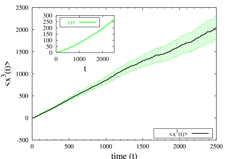
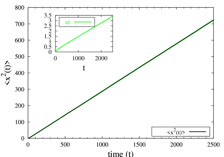
Figure 2: Evolution of $\langle x^{3}(t)\rangle$ (left) and $\langle x^{2}(t)\rangle$ (right) for $\delta=0.1$, $\gamma=0.3$ and $V_{\mbox{b}}=4$ (in units where $T=1$) with $8\cdot 10^{5}$ realizations. Statistical errors of one standard deviation are also included, together with their time evolution (small pictures). These grow as $t^{\frac{n}{2}}$ for $\langle x^{n}(t)\rangle$.

One immediately sees from figure 2 that $\langle x^{3}(t)\rangle$ grows linearly in time. In section 5 we obtained two possible long-time behaviours for $\langle x^{3}\rangle$, namely $\langle x^{3}\rangle=\mbox{constant}$ or $\langle x^{3}\rangle\sim t$. Therefore the numerical results support our arguments in favour of the latter for a periodic potential. The fact that it grows to a positive value is somewhat surprising since our equilibrium considerations showed that the velocity in the negative direction $v^{\downarrow}(\bar{\Theta})$ is larger than the velocity in the positive direction $v^{\uparrow}(\bar{\Theta})$ for $\delta_{\rm CP}>0$, so $\Delta v=v^{\uparrow}-v^{\downarrow}<0$. This behaviour for the asymmetry $\Delta v$ in the velocities is also found in our numerical simulations. It would seem to follow that $\langle x^{3}(t)\rangle$ evolves in time to a negative value. This is also supported by the random walk model considerations of appendix B. The numerical results however indicate the opposite, which means that probably non-equilibrium effects determine the sign of growth of $\langle x^{3}(t)\rangle$. It might also be that the sign depends on the details of the interactions, so that a different model could lead to a different sign.

Expectation values of higher powers of $x$ are dominated by their disconnected parts in the long time limit as argued in section 5. Therefore, according to equation (71) one has

$$f_{n}(t)\equiv\frac{\langle x^{2n+1}(t)\rangle}{\frac{(2n+1)!}{2^{n-1}\,3!(n-1)!}\langle x^{3}(t)\rangle\left[\langle x^{2}(t)\rangle\right]^{n-1}}\stackrel{{\scriptstyle t\rightarrow\infty}}{{\longrightarrow}}1.$$ (82)

We have explicitly checked this for $\langle x^{5}(t)\rangle$ and $\langle x^{7}(t)\rangle$ (figure (3) below).

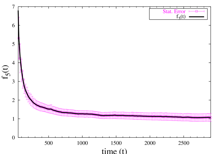
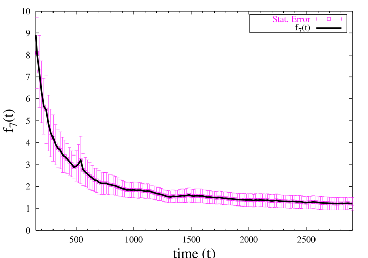
Figure 3: Evolution of $f_{5}(t)=\frac{\langle x^{5}(t)\rangle}{10\langle x^{3}(t)\rangle\langle x^{2}(t)\rangle}$ (left) and $f_{7}(t)=\frac{\langle x^{7}(t)\rangle}{105\langle x^{3}(t)\rangle\langle x^{2}(t)\rangle^{2}}$ (right).

In the case of $\langle x^{3}(t)\rangle$, its disconnected part $\langle x^{2}(t)\rangle\cdot\langle x(t)\rangle$ is negligible. This is because $\langle x(t)\rangle$ is constant in time and thus equal to $\langle x(0)\rangle$ which was chosen to be $\langle x(0)\rangle=0$ in our simulations. Actually in the numerical results $|\langle x\rangle|$ is of the order of $0.02\pm 0.1$. The large-time limit of $\langle x^{3}(t)\rangle$ in figure 2 corresponds therefore to its connected part.

We have also checked in the simulations that velocity expectation values $\langle v_{p}^{2n+1}\rangle$ have the limit given by (81). Thus we have verified that our stochastic model thermalizes in the way as expected in section 5.

7 On baryon-number generation from asymmetric Chern-Simons number diffusion

A natural question to ask is whether the asymmetric diffusion of the Chern-Simons number may yield a non-zero baryon number in some out-of-equilibrium situation. This section contains some remarks on this question. In particular, we will present a simple way in which asymmetric diffusion of a particle, with coordinate $x$, will lead to a (temporary) non-zero expectation value of $x$ itself. It is then argued that such a situation occurred during the electroweak phase-transition yielding a non-zero Chern-Simons number (and baryon number). In any electroweak baryogenesis scenario the two important questions are: Is the resulting baryon asymmetry sufficient to account for the observed asymmetry in the universe (1), and what are the requirements to prevent a wash out of the generated asymmetry? We will present some estimates to answer these questions.

Let us reconsider the diffusion of a particle in one dimension with coordinate $x$, that starts at $x=0$. As time evolves the distribution function will spread. In the long-time limit the distribution will become Gaussian with on top a small asymmetry (assuming that the symmetry-breaking terms are small). We have argued that $\langle x^{3}(t)\rangle$ grows linearly in time. To be definite, let us say it grows in the negative direction. Then the tail of the distribution in the negative-$x$ direction (-tail) will be larger than the tail of the distribution function in the positive-$x$ direction (+tail). This difference in the tails accounts for the negative values of $\langle x^{3}\rangle$ (and of expectation values of higher powers of $x$). That the expectation value of $x$ remains zero is due to an asymmetry in the distribution function closer to $x=0$. (A nice way to imagine this that the peak of the distribution function (the most probable position) moves in the positive-$x$ direction. The motion of the peak would give a growing $\langle x\rangle$ except that the contribution of the tails is precisely opposite. For higher powers of $x$ the tails dominate and a negative and growing value is the result.) With this picture of the evolution of the distribution function it is not hard to construct a system for which $\langle x\rangle$ itself becomes (temporarily) non-zero. All that one has to do is to prevent the -tail to compensate for the positive contribution of the peak moving in the positive-$x$ direction (if the peak does not move in the positive $x$-direction there is still a positive contribution from the region around $x=0$ and the argument goes through unchanged). Consider the diffusion of this particle in a box with symmetrically placed walls at $x=\pm a$. The -tail will hit the wall earlier than the +tail. Then the -tail can no longer compensate for the asymmetry of the distribution function close to $x=0$ (for instance the motion of the peak of the distribution function in the positive-$x$ direction). Hence, $\langle x\rangle$ will grow and become non-zero. Eventually, when the system goes to equilibrium, $\langle x\rangle$ relaxes back to zero.

Instead of putting the system in a box we could also have let the system evolve in a harmonic potential $V={\scriptstyle\frac{1}{2}}\omega^{2}x^{2}$ (to be superimposed on the periodic potential in which it diffuses). Basically by the same arguments as above it follows that the expectation value of $x$ becomes temporarily non-zero. A slightly more general case that may be considered, is a system that is initially in thermal equilibrium in the presence of a harmonic potential $V_{1}={\scriptstyle\frac{1}{2}}\omega_{1}^{2}x^{2}$ which changes at the initial time to $V_{2}={\scriptstyle\frac{1}{2}}\omega_{2}^{2}x^{2}$, with $\omega_{1}^{2}>\omega_{2}^{2}$. In the evolution towards the new equilibrium state, the expectation value $\langle x\rangle$ will temporarily become non-zero. In the next section we will show in a short-time expansion that $\langle x\rangle$ will become non-zero indeed, after such a change in a harmonic potential.

7.1 Short-time expansion

We show in the following that an instantaneous change from a potential $V_{1}=V_{\rm per}+{\scriptstyle\frac{1}{2}}\omega_{1}^{2}x^{2}$ to $V_{2}=V_{\rm per}+{\scriptstyle\frac{1}{2}}\omega_{2}^{2}x^{2}$, with $V_{\rm per}$ a periodic potential, will lead to a nonzero expectation value $\langle x\rangle$. We will use the Fokker-Planck equation (80), with $V_{2}$ as the potential, for the time evolution of the distribution function $P(p,x,t)$. The initial distribution function at time $t=t_{\rm in}$ is given by

$$P_{\rm in}(p,x)=Z^{-1}e^{-\beta[{\scriptstyle\frac{1}{2}}(p^{2}-\delta p^{3}+\delta^{2}p^{4})+V_{1}(x)]},$$ (83)

and the expectation value $\langle x\rangle$ by

$$\langle x(t)\rangle=\int dx\int dp\;x\,P(p,x,t).$$ (84)

We calculate this expectation value in a short-time expansion

$$\langle x(t)\rangle=\sum_{n}\frac{1}{n!}x_{n}t^{n},$$ (85)

with coefficients

$$x_{n}=\int dx\int dp\,x\,\left.\frac{\mbox{d}^{n}\mbox{ }}{\mbox{d}t^{n}}P(p,x,t)\right|_{t=t_{\rm in}}.$$ (86)

Define the operator

$$O=\partial_{p}\left[\gamma T\partial_{p}+\gamma v_{p}+(\partial_{x}V)\right]-v_{p}\partial_{x},$$ (87)

such that the Fokker-Planck equation (80) may be written as $\partial_{t}P=OP$, with potential $V=V_{2}$. The coefficients $x_{n}$ may be calculated by

$$x_{n}=\int dx\int dp\;x\,O^{n}P_{\rm in}(p,x).$$ (88)

The first three terms in the expansion (85) vanish

$$x_{0} = \langle x\rangle_{\rm in}=0,$$ (89)

$$x_{1} = \langle v_{p}\rangle_{\rm in}=0,$$ (90)

$$x_{2} = \langle(1-3\delta p)\partial_{x}V_{2}-\gamma v_{p}-3\delta\gamma(T-p^{2})\rangle_{\rm in}=0,$$ (91)

where

$$\langle\,..\,\rangle_{\rm in}=\int dx\int dp\,..\,P_{\rm in}(p,x).$$ (92)

For $x_{3}$ we find

$$x_{3}=3\delta\langle T\partial^{2}_{x}V_{2}-(\partial_{x}V_{2})^{2}\rangle_{\rm in}.$$ (93)

When $V_{2}=V_{1}$ this gives $x_{3}=0$. To first order in $\omega_{1}^{2}-\omega_{2}^{2}$ the result for $x_{3}$ is independent of the periodic potential, $V_{\rm per}$,

$$x_{3}=3\delta(\omega_{1}^{2}-\omega_{2}^{2})T.$$ (94)

This shows that a change in the potential will lead to a (temporary) non-zero value for $\langle x\rangle$, even if the initial and final potential is symmetric.

7.2 Numerical results

To obtain the behaviour of the evolution of $\langle x\rangle$ for longer times we numerically solve the stochastic model discussed in section 6, with the instantaneous potential change $V_{\rm{before}}=V_{\rm{b}}\sin^{2}(x)+{\scriptstyle\frac{1}{2}}\omega_{1}^{2}x^{2}\longrightarrow V_{\rm{after}}=V_{\rm{b}}\sin^{2}(x)+{\scriptstyle\frac{1}{2}}\omega_{2}^{2}x^{2}$ with $\omega_{1}^{2}$ and $\omega_{2}^{2}$ chosen to be equal to $0.1$ and $0.01$ respectively. The system is first let to be equilibrated in $V_{\rm{before}}$ and then the instantaneous potential quench is performed. The numerical results show that indeed a temporary non-zero value for $\langle x\rangle$ is obtained (see figure 4).

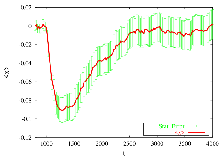
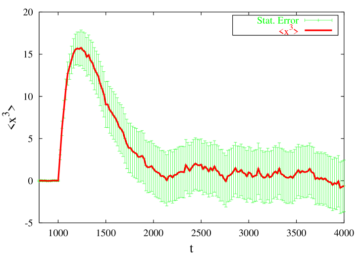
Figure 4: Evolution of $\langle x(t)\rangle$ (left) and $\langle x^{3}(t)\rangle$ (right) after the instantaneous potential change $V_{\rm{before}}\rightarrow V_{\rm{after}}$ (at $t\sim 1000$) with statistical errors included.

7.3 Baryon-number generation

We now turn to the problem of baryon-number generation. The back reaction of the generated baryons on the Chern-Simons number may be described by the effective potential given by the free energy at a given baryon-number $B$ [9, 10]

$$F(B)={\scriptstyle\frac{1}{2}}\omega_{B}^{2}B^{2}/V,$$ (95)

with $\omega_{B}^{2}=13/6T^{2}$ and $V$ the volume. Due to the relation between a change in the Chern-Simons number to a change in the baryon number, the effective potential generates a force on the Chern-Simons number. As a result a non-zero baryon number will be ”pushed back” to $B=0$ by the potential. This is the wash out of baryon number.

In terms of $\Theta$ the effective potential is given by

$$V_{\rm eff}(\Theta)=\frac{9}{2\pi^{2}}(gv)^{3}\omega_{B}^{2}\Theta^{2},$$ (96)

where the factor $(gv)^{3}$ is the inverse volume of a sphaleron.

Now consider the effect of a first-order electroweak phase-transition. Besides the complicated dynamics of bubble nucleation and moving bubble walls, the quarks will acquire a mass through the Higgs mechanism. This produces a small change in the back-reaction of the quarks on sphaleron transitions. In the description of this back-reaction in terms of an effective potential, this means that the potential (95) is changed by mass corrections: $\omega_{B}^{2}\rightarrow\omega_{B}^{2}(1-\sum_{i}c_{i}m_{i}^{2}/T^{2})$, with $m_{i}$ the masses of the different quark species and $c_{i}$ dimensionless coefficients. As argued before, a change in a (harmonic) potential will lead to a temporary non-zero value of the one-point function. Hence, the expectation value of the baryon and Chern-Simons number will acquire temporarily a non-zero value.

Before we discuss how ”temporarily” may become forever, we will turn to the question of how large we may expect the expectation value of the baryon number to grow. From the sample calculations in Appendix C, we learn that the asymmetry has typically a maximum value of $\sim(1-\omega_{2}^{2}/\omega_{1}^{2})\delta$, with $\delta$ a dimensionless measure of the amount of CP-violation and $\omega_{1}$ and $\omega_{2}$ the two frequencies of the potential before and after the phase transition. The factor $(1-\omega_{2}^{2}/\omega_{1}^{2})$, that is a measure of the amount of the departure from equilibrium, is of the order of the mass correction to the potential (95). Therefore, it is dominated by the top quark mass: $(1-\omega_{2}^{2}/\omega_{1}^{2})\sim m_{t}^{2}/6T^{2}$, with $m_{t}$ the top quark mass. In the case of Chern-Simons number diffusion we identify $\delta$ with the relative asymmetry in the velocity at the sphaleron configuration $\Delta v_{\rm rel,sph}$. Hence, when we consider the motion of $\Theta$ in this potential, we estimate for the maximum after the electroweak phase-transition

$$\langle\Theta\rangle_{\rm max}\sim\frac{m_{t}^{2}}{6T^{2}}|\Delta v_{\rm rel,sph}|.$$ (97)

Imagine the universe made up of blocks of size $(gv)^{-3}$ (the size of the sphaleron), with in each block a $\Theta$-variable. At the first-order electroweak phase-transition bubbles fill out the universe and in each block the harmonic potential for $\Theta$ changes. The time that the bubbles need to fill out the universe is much shorter than the time for a single sphaleron transition $(gv)^{3}\Gamma_{\rm sph}^{-1}$. Therefore, as far as the motion of $\Theta$ is concerned, the change in the potential occurs effectively at the same time in the whole universe. This implies that the expectation values of $\Theta$’s in different regions in the universe move simultaneously towards their maximum value. Then we get for the maximum baryon-number density, $n_{B}=\langle B\rangle/V$,

$$\left.\frac{n_{B}}{n_{\gamma}}\right|_{\rm max}\approx 4\frac{(gv)^{3}}{T^{3}}\langle\Theta\rangle_{\rm max},$$ (98)

with the photon density $n_{\gamma}=0.24\mbox{ }T^{3}$. In this estimate we used that $\Theta$’s in different blocks of space move independently, similar as in the case for pure diffusion in going from (55) to (56). This is only valid when the back reaction of the baryons on sphaleron transitions may be considered as arising from the potential (95) and non-localities may be neglected on the length scale $(gv)^{-1}$. This is what is usually done in the literature, see e.g. [18]. If this assumption is incorrect extra suppression factors may be expected.

When the generated baryon-number is not washed out, the asymmetry (98) results, at the present time, in an asymmetry

$$\left.\frac{n_{B}}{n_{\gamma}}\right|_{\rm max,now}\approx\left[7\,\delta^{1}_{\rm CP}+6\,\delta^{2}_{\rm CP}\right]10^{-4}\;\left(\frac{100\mbox{ GeV}}{M}\right)^{4},$$ (99)

where we used $g=0.6,m_{t}=170\mbox{ GeV},\mbox{ and }v\sim T\sim 100\mbox{ GeV}$. This rough estimate for the asymmetry may indicate that in the process considered here, sufficient baryons may have been generated, provided that the CP-violation is strong enough and occurs at a not-too-high energy-scale. It may be noted that the mass $M$, that gives the energy scale of new physics, may not be as large as in scenario’s for baryon generation based on CP-violation through CP-odd dimension-six operators, since (99) is suppressed by four powers of $M$ (instead of two). Other constraints for the scenario based on asymmetric diffusion may be more important and are discussed in the next section.

7.4 Constraints

The immediate question is whether a once created baryon asymmetry survive to present times. The decay of the baryon-number density, $n_{B}$, for small densities is given by [9]

$$\frac{\mbox{d}n_{B}}{\mbox{d}t}=-9\beta\omega_{B}^{2}\Gamma_{\rm sph}n_{B}$$ (100)

The formal solution is

$$n_{B}(t)=n_{B}(t_{\rm pt})e^{-R(t)},$$ (101)

with

$$R(t)=9\int_{t_{\rm pt}}^{t}dt^{\prime}\beta\omega_{B}^{2}\Gamma_{\rm sph}(t^{\prime}),$$ (102)

with $t_{\rm pt}$ the time of the electroweak phase-transition and $\Gamma_{\rm sph}(t)$ the time-dependent sphaleron rate (its time-dependence enters through the changing temperature and Higgs expectation value as the universe cools down). The requirement that a generated baryon asymmetry survives to present times is

$$R=R(\infty)\lesssim 1.$$ (103)

This may be translated into a bound on the phase transition strength

$$v_{\rm pt}>v_{\rm cr}\sim 100\mbox{ GeV},$$ (104)

with $v_{\rm pt}$ the Higgs expectation value just after the first-order electroweak phase transition.

In [20] one of the authors believed that the bound to prevent the wash out of baryon number could be much weaker. This was based on the realization that that the linear response result is not directly applicable to the situation where a non-zero expectation value of a coordinate is generated by asymmetric diffusion in a symmetric potential. (Since according to linear response this expectation value can never become non-zero, which as was seen in section 7.1, is not the case.) However the time scale for equilibration given by linear response (101) is still correct. Therefore, the bound (103) still applies.

In the scenario discussed there is another bound, since the asymmetry itself has to be generated after the phase transition. Therefore, to generate a large asymmetry sufficient sphaleron transitions must occur after the phase transition. This requires

$$R\gtrsim 1.$$ (105)

Hence, to generate sufficient baryons without a large wash out in the scenario that we discuss here, the number of sphaleron transitions after the phase transition has to lie in a small range around $1$. We expect typically something like

$$e^{-1}<R<e.$$ (106)

This requirement for the number of sphaleron transitions after the electroweak phase-transition may be translated into a requirement on the strength of the phase transition, that may be indicated by the Higgs expectation value just after the transition, $v_{\rm pt}$. In appendix D we show that from (106) it follows that this Higgs expectation value lies in the range

$$v_{\rm cr}\left(1-\frac{1}{\beta_{\rm pt}E_{\rm sph}}\right)<v_{\rm pt}<v_{\rm cr}\left(1+\frac{1}{\beta_{\rm pt}E_{\rm sph}}\right),$$ (107)

with the inverse inverse temperature at the phase transition $\beta_{\rm pt}\sim(100\mbox{ GeV})^{-1}$. Since, $\beta_{\rm pt}E_{\rm sph}\sim 45$ the range of allowed phase transition strengths is quite small. Hence, for the above scenario for the generation of matter to work, the strength of the electroweak phase transition has to satisfy strict bounds (107). For a given particle model these bounds may be translated into bounds for the Higgs mass, as has already been done for the bound (103) or (104) for the minimal supersymmetric standard model [21],[22],[23].

7.5 Discussion

Perhaps it is useful to consider the difference between the effect of the dimension-six operator $\phi^{\dagger}\phi F\tilde{F}$ (the lowest-dimensional CP-odd operator) and the dimension-eight operators $(D\phi)^{\dagger}(D\phi)F\tilde{F}$ and $(FF)(F\tilde{F})$ in the context of electroweak baryogenesis. As we have argued the dimension-six operator does not affect the diffusion of the Chern-Simons number in equilibrium. However in a non-equilibrium situation it may have an effect. In particular, when the Higgs expectation value changes in time the dimension-six operator introduces an effective force $F_{\rm eff}\sim\partial_{t}\langle\phi^{\dagger}\phi\rangle$ on the motion of the Chern-Simons number. This implies that in the case of a time-dependent Higgs expectation value the diffusion of the Chern-Simons number yields a non-zero expectation value of $N_{\rm CS}$ itself: $\langle[N_{\rm CS}(t)-N_{\rm CS}(0)]\rangle\sim\Gamma_{\rm sph}F_{\rm eff}t$. This in contrast to the asymmetry generated by the dimension-eight operators in equilibrium that affect only expectation values of third and higher powers of $N_{\rm CS}(t)-N_{\rm CS}(0)$.

It is well-known that the dimension-six operator may play a role in the generation of the baryon asymmetry. For instance, during the electroweak phase-transition when the Higgs expectation value grows the effective force can be used to push the Chern-Simons number and baryon number to some positive value. The problem is that during the growth of the Higgs expectation value the sphaleron rate decreases. Therefore it is difficult to generate a sufficient baryon asymmetry in the short time that the Higgs expectation grows. A way to circumvent this problem has been given in [15]. In that paper the situation was considered that the reheating temperature after inflation is below the temperature at which the electroweak phase-transition takes place. This means that there never was an electroweak phase-transition. The Higgs expectation value grows during the reheating of the universe. At this time the CP-odd dimension-six operator generates the earlier mentioned effective force. Further it has been argued in [15] that during the period of reheating the exponential suppression of the sphaleron rate is absent. Therefore sufficient sphaleron transitions can take place and a baryon asymmetry may be generated. Since the sphaleron rate becomes exponentially suppressed when the plasma thermalizes, a generated baryon asymmetry may be preserved.

When the asymmetric diffusion of the Chern-Simons number from CP-odd dimension-eight operators plays a role in the generation of a baryon asymmetry, as we have argued is possible, then the time-scales for the generation and the wash out of a baryon asymmetry are similar. Therefore there is no need to try to avoid the exponential suppression of the sphaleron rate. The price to pay is for these similar time scales is that the strength of the phase transition needs to be finely tuned in order to ensure sufficient sphaleron transitions after the phase-transition and avoid a subsequent wash out of baryon number (see section 7.4).

Of course, in section 7 we have neglected various important dynamical aspects of the problem. Such as the motion of the bubble walls of a first-order phase transition, the motion of the baryons and dynamical aspects of their back-reaction on the motion of the Chern-Simons number, the growth in energy of sphaleron configuration as a bubble wall passes a certain region in space (that is as the Higgs expectation value increases), the non-Brownian beginning of the motion of the Chern-Simons number [24] etc. These neglected aspects may well modify the here presented estimate for the final baryon asymmetry. It is even possible that, being non-equilibrium processes, one of these will provide, in combination the included CP-violation, a different mechanism for baryon number generation. If so, the dimension-eight operators in (4) may prove more effective than the dim-six operator in (3) in providing the necessary CP-violation when the Higgs expectation value is not rapidly changing. Although all these non-equilibrium phenomena could yield a non-zero baryon number in combination with CP-violation, we believe that the mechanism presented in section (7) is the most natural way to generate an asymmetry on the basis of the CP-odd dimension-eight operators.

8 Summary

We have argued that the inclusion of CP-odd operators, especially the dimension-eight operators in (4), in an effective action will result in an asymmetric diffusion of the Chern-Simons number (in the absence of fermions). That is, in thermal equilibrium the correlation function $\langle[N_{\rm CS}(t)-N_{\rm CS}(0)]^{3}\rangle$ becomes nonzero. In section 5, we noted that, on general grounds, the expectation value of the third power of a coordinate either grows linearly in time or goes to a constant in the long time limit. We have argued that in the broken phase $\langle[N_{\rm CS}(t)-N_{\rm CS}(0)]^{3}\rangle$ grows linearly in time. A more detailed conjecture was given in (56). Unfortunately, the study presented here did not allow us to determine the sign of the expectation value (the direction of the growth).

Further we noted that asymmetric diffusion may lead to a non-zero expectation value of the coordinate itself in a non-equilibrium situation. For instance when the potential is changed (even if before, during, and after the change the potential is symmetric). This may have implications for the generation of the baryon asymmetry in the early universe. Although there are severe constraints on the strength of the electroweak phase-transition, we found that the observed baryon asymmetry could be generated by asymmetric diffusion in combination with the electroweak phase-transition.

Acknowledgements

We would like to thank Jan Smit and Jeroen Vink for useful comments and discussions. A.A. was supported by Foundation FOM of the Netherlands.

Appendix A Relation between the Chern-Simons number and $\Theta$

The change in the Chern-Simons number is given by

$$N_{\rm CS}(t)-N_{\rm CS}(0)=\frac{g^{2}}{32\pi^{2}}\int_{0}^{t}dt^{\prime}\int d^{3}xF_{\mu\nu}^{a}\tilde{F}^{\mu\nu a}.$$ (108)

Using the parametrization (9) of the non-contractable loop in configuration space found by Manton [12], equation (108) may be rewritten in terms of $\Theta$:

$$N_{\rm CS}(t)-N_{\rm CS}(0)=\frac{12}{\pi}\int_{0}^{t}dt^{\prime}\dot{\Theta}\sin^{2}\Theta\int_{0}^{\infty}dr(\partial_{r}f)f(1-f).$$ (109)

The time and spatial integrations may be factorized. The spatial integration is completely determined by the boundary values of the function $f$ (it does therefore not depend on the Ansatz that is made for $f$, given the boundary conditions)

$$\int_{0}^{\infty}dr(\partial_{r}f)f(1-f)=\frac{1}{6}.$$ (110)

Hence, the relation between the change in Chern-Simons number and $\Theta$ is given by

$$N_{\rm CS}(t)-N_{\rm CS}(0)=\frac{2}{\pi}\int_{0}^{t}dt^{\prime}\dot{\Theta}\sin^{2}\Theta.$$ (111)

For instance when we change $\Theta$ from $\Theta(0)=0$ to $\Theta(t)=n\pi$, crossing $n$ barriers, the Chern-Simons changes as

$$N_{\rm CS}(t)-N_{\rm CS}(0)=n,$$ (112)

as expected.

Appendix B Random walk model

A random walk model is a convenient toy model to study diffusion. For asymmetric diffusion we consider a one-dimensional random walk model with probabilities

$$P_{R}=(1+\Delta)/2,\;P_{L}=(1-\Delta)/2,$$ (113)

of moving right ($R$) or left ($L$). The distance the particle moves in one time step differs also between the two different directions. When the particle moves to the right it travels a distance $\Delta x_{R}$ and when it moves to the left a distance $\Delta x_{L}$:

$$\Delta x_{R}=(1+\Delta)^{-1},\;\Delta x_{L}=(1-\Delta)^{-1}.$$ (114)

The relation

$$P_{R}\Delta x_{R}-P_{L}\Delta x_{L}=0,$$ (115)

implies that the flux vanishes.

Thus, the random walk model defined above contains the two important features of the motion of the Chern-Simons number established in section 3. The flux vanishes (at every point), see (47), and the left and right velocities differ, see (53), which translates in the different distances (114) travelled in one time step in the random walk model.

The distribution function of the number of steps to the right, $R$ and the number of steps to the left,$L$, after a total of $N=L+R$ steps, reads

$$P(L,R,N)=\delta_{L+R,N}\frac{N!}{L!R!}\frac{1}{2^{N}}(1-\Delta)^{L}(1+\Delta)^{R}.$$ (116)

When the particle starts at the initial time, $N=0$, at position $x=0$, $x$ is given by

$$x=R\Delta x_{R}-L\Delta x_{L}.$$ (117)

The relation $L+R=N$ and (117) can be used to convert (116) in a distribution function of $x$. Instead, we will calculate expectation values. Let us start with $\langle x\rangle$. As mentioned before, the vanishing of the flux should imply that $\langle x\rangle$ is constant and, since the particle starts at $x=0$, is zero. This may be checked for the random walk model. The expectation value of $x$ is given by

$$\langle x(N)\rangle = \sum_{L=0}^{N}\sum_{R=0}^{N}\delta_{L+R,N}\frac{N!}{L!R!}\frac{1}{2^{N}}(1-\Delta)^{L}(1+\Delta)^{R}$$ (118)

$$\times\left[R(1+\Delta)^{-1}-L(1-\Delta)^{-1}\right].$$

We define $R^{\prime}=R-1$ and $L^{\prime}=L-1$ and write (118) as

$$\langle x(N)\rangle = \sum_{L=0}^{N}\sum_{R^{\prime}=0}^{N-1}\delta_{L+R^{\prime},N-1}\frac{N!}{L!R^{\prime}!}\frac{1}{2^{N}}(1-\Delta)^{L}(1+\Delta)^{R^{\prime}}$$ (119)

$$- \sum_{L^{\prime}=0}^{N-1}\sum_{R=0}^{N}\delta_{L^{\prime}+R,N-1}\frac{N!}{L^{\prime}!R!}\frac{1}{2^{N}}(1-\Delta)^{L^{\prime}}(1+\Delta)^{R}.$$

Since in the first line on the right hand side of (119) the term $L=N$ in the sum over $L$ does not contribute due to the delta function, and similarly the term $R=N$ does not contribute in the second line, the sums in the first and second line cancel. Hence

$$\langle x(N)\rangle=0,$$ (120)

in accord with (47).

Next, consider the expectation value

$$\langle x^{3}(N)\rangle = \sum_{L=0}^{N}\sum_{R=0}^{N}\delta_{L+R,N}\frac{N!}{L!R!}\frac{1}{2^{N}}(1-\Delta)^{L}(1+\Delta)^{R}$$ (121)

$$\times\left[R(1+\Delta)^{-1}-L(1-\Delta)^{-1}\right]^{3}.$$

This expression may be evaluated in a similar manner as (118). The result is

$$\langle x^{3}(N)\rangle=\frac{1}{2}N\left[(1+\Delta)^{-2}-(1-\Delta)^{-2}\right].$$ (122)

Hence, for positive $\Delta$, the expectation value $\langle x^{3}\rangle$ is negative and grows linearly in time.

This calculation supports our argument that when the asymmetry is independent of space and constant in time the expectation value $\langle x^{3}\rangle$ grows linearly in time.

Appendix C Some solutions to the stochastic equation

In this appendix we present some calculations using the Langevin equation (74) with a constant potential or a harmonic potential.

We start with a calculation of $\langle x\rangle$ in the case $V=0$. The Langevin equation (74) with $V=0$ reads

$$\ddot{x}\left(1+3\delta\dot{x}+6\delta^{2}\dot{x}^{2}\right)=-\gamma\dot{x}+\xi,$$ (123)

with

$$\langle\xi(t)\rangle_{\xi} = 0,$$ (124)

$$\langle\xi(t)\xi(t^{\prime})\rangle_{\xi} = 2\gamma T\delta(t-t^{\prime}),$$ (125)

and initial conditions $x(0)=x_{\rm in}$, $\dot{x}=v_{\rm in}$.

We solve the equations of motion in an expansion in $\delta$:

$$x(t)=x_{0}(t)+\delta x_{1}(t)+...,$$ (126)

where $x_{0}$ and $x_{1}$ satisfy the equations

$$\ddot{x}_{0} = -\gamma\dot{x}_{0}+\xi,$$ (127)

$$\ddot{x}_{1} = -\gamma\dot{x}_{1}-3\dot{x}_{0}\ddot{x}_{0},$$ (128)

with initial conditions

$$x_{0}(0)=x_{\rm in}, \dot{x}_{0}(0)=v_{\rm in},$$ (129)

$$x_{1}(0)=0, \dot{x}_{1}(0)=0.$$ (130)

The solution for $x_{0}$ reads

$$x_{0}(t)=x_{\rm in}+\frac{v_{\rm in}}{\gamma}(1-e^{-\gamma t})+\int_{0}^{t}dt^{\prime}G(t-t^{\prime})\xi(t^{\prime}),$$ (131)

with the Green function $G(t-t^{\prime})=[1-e^{-\gamma(t-t^{\prime})}]/\gamma$. The solution for $x_{1}$ is

$$x_{1}(t)=-3\int_{0}^{t}dt^{\prime}G(t-t^{\prime})\dot{x}_{0}(t^{\prime})\ddot{x}_{0}(t^{\prime}).$$ (132)

When the average over the stochastic force is performed, we obtain

$$\langle x_{0}(t)\rangle_{\xi} = x_{\rm in}+\frac{v_{\rm in}}{\gamma}(1-e^{-\gamma t}),$$ (133)

$$\langle x_{1}(t)\rangle_{\xi} = \frac{3}{\gamma}[v_{\rm in}^{2}-T](\frac{1}{2}-e^{-\gamma t}+e^{-2\gamma t}).$$ (134)

We take thermal initial conditions: $x_{\rm in}=0$ and $v_{\rm in}$ is thermally distributed. The average over initial momenta gives for the initial velocity and velocity squared

$$\langle v_{\rm in}\rangle_{\rm in}=0,\;\langle v_{\rm in}^{2}\rangle=T+{\cal O}(\delta).$$ (135)

Hence the average over initial conditions of (133) and (134) gives

$$\langle\langle x_{0}(t)\rangle_{\xi}\rangle_{\rm in} = 0,$$ (136)

$$\langle\langle x_{1}(t)\rangle_{\xi}\rangle_{\rm in} = {\cal O}(\delta).$$ (137)

Therefore the combined thermal and stochastic average of $x$ vanishes,

$$\langle\langle x(t)\rangle_{\xi}\rangle_{\rm in}=0,$$ (138)

up to order $\delta$.

This is an explicit check that when the velocity is thermally distributed, and hence $\langle\dot{x}\rangle=0$, that then $\langle x(t)\rangle=\mbox{constant}$.

The second quantity that we have calculated is $\langle x^{3}(t)\rangle_{\xi}$. We find that it goes to a constant (that depends on the initial distribution) in the long time limit. For the initial conditions $x_{\rm in}=0$ and $v_{\rm in}$ thermally distributed, we find

$$\langle\langle x^{3}(t)\rangle_{\xi}\rangle_{\rm in}\rightarrow-\frac{21}{2\gamma}\delta\left(\frac{T}{\gamma}\right)^{2}.$$ (139)

Hence, differently than we have argued for the diffusion of the Chern-Simons number, in this case the expectation value of the third power does not grow linearly in time. Since there are no high barriers, we don’t expect the velocity to thermally distributed, independent of the position in space. Therefore the asymmetry in the velocities does not need to be independent of the position in space. In this way the argument for the linear growth of the expectation of $x^{3}(t)$ does not hold in this case. Hence, the fact that $\langle x^{3}(t)\rangle$ goes to a constant when $V=0$, does not contradict the expected linear growth of $\langle[N_{\rm CS}(t)-N_{\rm CS}(0)]^{3}\rangle$ in the long time limit. It does raise the following question. When we add a periodic potential $V_{\rm b}\sin^{2}(x)$, how does the long time behavior of $\langle x^{3}(t)\rangle$ depend on $V_{\rm b}$? We know that for $V_{\rm b}=0$ it goes to a constant, and we have argued that for $V_{\rm b}/T>>1$ it grows linearly in time. So, at what value of $V_{\rm b}$ does the behavior change?

Next, we consider the time-evolution in a harmonic potential $V={\scriptstyle\frac{1}{2}}\omega_{2}^{2}x^{2}$. As initial distribution we use for the position $\exp-\beta{\scriptstyle\frac{1}{2}}\omega_{1}^{2}x_{\rm in}^{2}$ and $v_{\rm in}$ is thermally distributed. This situation may be viewed as follows. The system is in thermal equilibrium before the initial time, $t=0$, with a potential $V={\scriptstyle\frac{1}{2}}\omega_{1}^{2}x^{2}$. At the initial time the harmonic potential changes ${\scriptstyle\frac{1}{2}}\omega_{1}^{2}x^{2}\rightarrow{\scriptstyle\frac{1}{2}}\omega_{2}^{2}x^{2}$. We calculate the following time evolution of $\langle x\rangle$. In the case without damping, $\gamma=0$, We get to first order in $\delta$

$$\langle x(t)\rangle=\frac{\delta T}{\omega_{2}}\left(1-\frac{\omega_{2}^{2}}{\omega_{1}^{2}}\right)\sin(\omega_{2}t)[1-\cos(\omega_{2}t)].$$ (140)

For the case $\gamma>>\omega$, we present only the contribution of the slowest decaying mode

$$\langle x(t)\rangle=-\frac{3\delta T\omega_{2}^{2}}{2\gamma^{3}}\left(1-\frac{\omega_{2}^{2}}{\omega_{1}^{2}}\right)e^{-(\omega_{2}^{2}/\gamma)t}+{\cal O}(e^{-2(\omega_{2}^{2}/\gamma)t}).$$ (141)

We learn from (140) and (141) that the expectation value $\langle x\rangle$ becomes non-zero after the potential is changed, as we have argued in section 7. And further that the magnitude of $\langle x\rangle$ is proportional to $(1-\omega_{2}^{2}/\omega_{1}^{2})$ and $\delta$.

Appendix D Bound on the strength of the phase transition

In this appendix we show how the bound (106)

$$e^{-1}<R<e,$$ (142)

with

$$R=9\int_{t_{\rm pt}}^{\infty}dt^{\prime}\beta\omega_{B}^{2}\Gamma(t^{\prime}),$$ (143)

may be translated into a bound on the Higgs expectation immediately after the electroweak phase transition, $v_{\rm pt}$.

In order to simplify the following calculations we take $\kappa$ in (7) to be constant, then

$$9\beta\omega_{B}^{2}\Gamma_{\rm sph}=\frac{39}{2}\kappa Te^{-\beta E_{\rm sph}}.$$ (144)

As a further simplifying approximation, we will assume that the Higgs expectation value stays constant after the phase transition and that the only time dependence enters through the temperature as [25]

$$T^{2}=0.03\frac{M_{\rm pl}}{t},$$ (145)

where $M_{\rm pl}=1.2\mbox{ }10^{19}$ GeV is the Planck mass.

When the Higgs expectation value, $v$, is time-independent so is the sphaleron energy $E_{\rm sph}$, and the integration in (143) can easily be performed. The result is

$$R=K\frac{M_{\rm pl}}{E_{\rm sph}}e^{-\beta_{\rm pt}E_{\rm sph}},$$ (146)

with $K=1.08\;\kappa$ and $\beta_{\rm pt}$ the inverse temperature at the electroweak phase-transition.

It is useful to determine the value $v_{\rm pt}=v_{\rm cr}$ for which

$$R=1.$$ (147)

Inserting the result (146) for $R$ and taking the natural logarithm gives

$$\ln R=\ln K\frac{M_{\rm pl}}{E_{\rm sph}}-\beta_{\rm pt}E_{\rm sph}=0.$$ (148)

From [9] we obtain the value for $\kappa=1.3\mbox{ }10^{4}$. Inserting this value for $\kappa$ in $K$ and then in (148) yields

$$\beta_{\rm pt}E_{\rm sph}=45.$$ (149)

This gives for the phase transition strength

$$v_{\rm cr}\sim T_{\rm pt}\sim 100\mbox{ GeV}.$$ (150)

In [11] the time- or temperature-dependence of the Higgs expectation value is taken into account in the derivation of $v_{\rm cr}$. We are more interested in the window of phase-transition strengths determined by (142).

A small shift of $v_{\rm pt}$ by an amount of $\delta v$, $v_{\rm pt}=v_{\rm cr}+\delta v$, saturates the lower bound in (142)

$$R(v_{\rm cr}+\delta v)=e^{-1}.$$ (151)

This equation gives for $\delta v$

$$\frac{\delta v}{v_{\rm cr}}(1-\beta_{\rm pt}E_{\rm sph})=-1.$$ (152)

Thus the bound (142) translates into the following bound for the phase-transition strength $v_{\rm pt}$

$$v_{\rm cr}\left(1-\frac{1}{\beta_{\rm pt}E_{\rm sph}}\right)<v_{\rm pt}<v_{\rm cr}\left(1+\frac{1}{\beta_{\rm pt}E_{\rm sph}}\right),$$ (153)

for $\beta_{\rm pt}E_{\rm sph}>>1$.

References

- [1] K. Olive, Nucl. Phys. Proc. Suppl. 80 (2000) 79.
- [2] A. D. Sakharov, JETP Lett. 5 (1967) 24.
- [3] G. ’t Hooft, Phys. Rev. Lett. 37 (1976) 8.
- [4] V. Kuzmin, V. Rubakov, and M. Shaposhnikov, Phys. Lett. B155 (1985) 36.
- [5] V. Rubakov and M. Shaposhnikov, Phys. Usp. 39 (1996) 461.
- [6] P. Arnold, D. Son, and L. Yaffe, Phys. Rev. D55 (1997) 6264.
- [7] D. Bödeker, Phys. Lett. B426 (1998) 169.
- [8] D. Bödeker, G. Moore, and K. Rummukainen, D61 (2000) 056003.
- [9] P. Arnold and L. McLerran, Phys. Rev. D36 (1987) 581.
- [10] S. Khlebnikov and M. Shaposhnikov, Nucl. Phys. B308 (1988) 885.
- [11] G.D. Moore, Phys. Rev. D59 (1999) 014503.
- [12] N. S. Manton, Phys. Rev. D28 (1983) 2019.
- [13] T. Akiba, H. Kikuchi, and T. Yanagida, Phys. Rev. D38 (1988) 1937.
- [14] F. Klinkhamer and N. S. Manton, Phys. Rev. D30 (1984) 2212.
- [15] J. Garcia-Bellido, D. Yu. Grigoriev, A. Kusenko, and M. Shaposhnikov, Phys Rev D60 (1999) 123504.
- [16] J. Zinn-Justin, Quantum Field Theory and Critical Phenomena (Clarendon, Oxford, 1989).
- [17] Ya. Sinai, Topics in Ergodic Theory, (Princeton University Press, 1994).
- [18] M. Joyce, T. Prokopec, and N. Turok, Phys. Rev. D53 (1996) 2930, Phys Rev D53 (1996) 2957.
- [19] R. P. Feynman and A. Hibbs, Quantum Mechanics and Path Integrals (McGraw-Hill, 1965)
- [20] B. J. Nauta, Phys. Lett. B478 (2000) 275.
- [21] J.M. Moreno, M. Quiros, and M. Seco, Nucl. Phys. B526 (1998) 489.
- [22] J.M. Cline and G. D. Moore, Phys. Rev. Lett. 81 (1998) 3315.
- [23] M. Laine and K. Rummukainen, Nucl. Phys. B597 (2001) 23.
- [24] A. Rajantie, P.M. Saffin, and E.J. Copeland, Phys. Rev. D63 (2001) 123512.
- [25] E. Kolb and M. Turner, The early universe, (Addison-Wesley, 1989).