Precision Test of Quark Mass Textures: A Model Independent Approach

Abstract

Using a Monte Carlo method, we have directly extracted from the available measurements, the hierarchies among the different elements of the quark mass matrices. To do that, we have first introduced a model independent parameterization for two generic class of models: those based on Abelian symmetries and those inspired by a $U(2)$ horizontal symmetry. So, matrix entries are proportional to some $\epsilon^{t}$, with $\epsilon<<1$ and the $t$’s are different free exponents that we determine from the data through a statistically well defined procedure. We have found that the experimental data poorly constrain the Abelian scenarios.

Instead, in non Abelian scenarios, these $t$-exponents are strongly constrained by the present data.We have found that contrary to a naive $U(2)$ horizontal symmetry expectation,  quark mass matrices turn out to be not symmetric. Two solutions emerge: one with $M_{32}^{{\rm down}}\gg M_{23}^{{\rm down}}$ and $M_{21}^{{\rm up}}\gg M_{12}^{{\rm up}}$ ; and a second one with slight asymmetries only in the light quark sector, namely $M_{21}^{{\rm up}}<M_{12}^{{\rm up}}$ and $M_{21}^{{\rm down}}>M_{12}^{{\rm down}}$ .

IFUM-702-FT

1 Introduction

Standard Model predictions have been tested so far with very high accuracy (at the permill level), and the agreement with the experimental measurements is very remarkable. However the Standard Model is unsatisfactory since all fermion masses and mixings are free and unpredictable parameters. Quark masses vary in a range of more than four order of magnitudes and the lack for an explanation is deceiving.
If the Higgs boson is a $SU(2)$ doublet, the four real components

$$\Phi=\pmatrix{\phi_{1}+\mathrm{i}\phi_{2}\cr\phi_{3}+\mathrm{i}\phi_{4}}$$ (1)

can be transformed by an $SO(4)\equiv SU(2)_{{\rm left}}\times SU(2)_{{\rm right}}$ symmetry. The unique $SU(2)$ invariant $\Phi^{\dagger}\Phi=\phi_{1}^{2}+\phi_{2}^{2}+\phi_{3}^{2}+\phi_{4}^{2}$ is also an $SO(4)$ invariant. The Higgs potential must be a $SO(4)$ invariant, and when the $SU(2)\times U(1)$ symmetry is broken into $U(1)_{em}$, the $SO(4)$ symmetry is broken into $SU(2)_{V}=SU(2)_{{\rm left+right}}$. The Goldstone bosons of the Higgs doublet transform as a triplet under the unbroken $SU(2)_{V}$ and this directly implies a fundamental relation between the mixing angle of the neutral gauge bosons and the charged/neutral boson masses [1]

$$1-\frac{M_{W}^{2}}{M_{Z}^{2}}=\sin^{2}\theta_{W}.$$ (2)

The remarkable experimental success of this relation which has been proved by the precision tests at $LEP$ and $SLD$, makes the above $SO(4)$ symmetry unique and unavoidable for any realistic description of the electroweak symmetry breaking. The same success is far from being achieved in the fermion sector, because there are too many models and symmetries which roughly give acceptable predictions (i.e. in terms of order of magnitudes). The large number of fermions and the lack of direct measurements of all the mass matrix entries make particularly hard to unambiguously select the underlying symmetries responsible for fermion mass hierarchies: measuring the CKM matrix elements, one fixes only the product of two unitary matrices, coming from the separate diagonalizations of the up and down $3\times 3$ quark mass, and not both of them.
To cope with these ambiguities, one usually assumes a fundamental symmetry and chooses a breaking pattern. The mass matrices obtained are diagonalized. Eigenvalues and eigenvectors are compared with the experimental data, ı.e. the CKM parameters and the quark masses. This procedure can be used to rule out a model or a symmetry if theoretical predictions and experimental data disagree. It is, of course, unable to prove that the assumed symmetry is the one which is preferred by the data. Ideally one could take a completely model independent approach and prove that a symmetry is among the best ones that can predict the correct mixings and masses spectrum. This goal is probably unachievable, but a step in this direction can be done if one accepts a certain amount of model dependence, selecting a large class of models, and then extracting directly from experimental results the preferred models within that class.

In the following, we explicitly discuss how to approach this goal, introducing model independent parameterizations for the up and down quark mass matrices. The needed number of free parameters  will be in general larger than the number of experimental constraints and this will be the main limitation for a direct fit of parameter values. Instead of minimizing the $\chi^{2}$  with respect to the full set of  free parameters (which is too large to be manageable), we get rid of several unknown parameters, treating them as real theoretical errors, through a Monte Carlo procedure.

To exemplify the proposed method, we will focus on two different parameterizations inspired by two classes of models: those based on Abelian symmetries and those exploiting a horizontal $U(2)$ symmetry.

2 The experimental constraints

Values of the six quark masses and of the four CKM matrix element parameters, used in the present analysis are given in Tables 1 and 2.

Quark flavour	Reference value	$\overline{m}_{q}(m_{W})$
	GeV/c2	GeV/c2
top	${\rm M}^{pole}_{t}=174.3\pm 5.1$	$175.3\pm 5.1\pm 0.2$
bottom	$\overline{m}_{b}(\overline{m}_{b})=4.19\pm 0.05$	$2.906\pm 0.035\pm 0.031$
charm	$\overline{m}_{c}(\overline{m}_{c})=1.304\pm 0.027$	$0.667\pm 0.014\pm 0.023$
strange	$\overline{m}_{s}(m_{\tau})=0.125\pm 0.030$	$0.072\pm 0.017\pm 0.002$
up and down quarks	Reference values	$\overline{m}_{q}(m_{W})~{}{\rm MeV/c^{2}}$
	$\frac{m_{u}}{m_{d}}=0.46\pm 0.09$	$\overline{m}_{d}(m_{W})=3.7\pm 0.9$
	$Q^{2}=\frac{4m_{s}^{2}-(m_{u}+m_{d})^{2}}{4(m_{d}^{2}-m_{u}^{2})}=22.0\pm 0.6$	$\overline{m}_{u}(m_{W})=1.7\pm 0.5$

Table 1: Values of quark masses used in this analysis. The second column gives the reference values from which they are evolved using the $\overline{{\rm MS}}$ scheme. For quarks heavier than $u$ and $d$ the last column gives the values extrapolated at the scale of the W boson mass, the first uncertainty corresponds to the uncertainty on the reference values and the second uncertainty is due to the extrapolation. Uncertainties quoted for $u$ and $d$-quark flavours are only indicative as mass ratios are directly determined.

CKM parameter	Reference value
$\lambda$	$0.2237\pm 0.0033$
$\left|{\rm V}_{cb}\right|$	$(41.0\pm 1.6)\times 10^{-3}$
$\rho$	$0.225\pm 0.038$
$\eta$	$0.317\pm 0.041$

Table 2:  Values of the CKM matrix parameters used in the present analysis [15].

2.1 Quark mass determinations

Values of quark masses span a large domain ranging from a few MeV/c², for $u$ and $d$ flavours, to more than 100 GeV/c² for the top quark. Current quark masses, defined in the $\overline{{\rm MS}}$ scheme have been used and their values have been given at the scale of the W mass. It can be noted that the present analysis depends on quark mass ratios and that these quantities are almost scale independent. The running of quark masses has been evaluated following the work of [3]. The value adopted for the strong coupling constant, at the scale of the ${\rm Z}$ boson mass is $\alpha_{s}(m_{Z})=0.1181\pm 0.0020$ which corresponds to $\Lambda^{(5)}=209.5^{+24.4}_{-22.6}$ MeV in the $\overline{{\rm MS}}$ scheme.

The top-quark mass has been measured from the direct reconstruction of its decay products [4]. It corresponds to the pole mass value:

$${\rm M}^{pole}_{t}=(174.3\pm 5.1)~{}{\rm GeV/c}^{2}.$$ (3)

The expression relating $\overline{m}_{t}({\rm M}^{pole}_{t})$ and ${\rm M}^{pole}_{t}$ can be found in [3].

Lattice determinations of the $b$ and $c$ quark masses can be found in [5]. The $b$-quark mass is obtained using QCD sum rules for the $\Upsilon$ masses and electronic widths following the work of [6]. Recent evaluations and complete references can be found in [7] giving:

$$\overline{m}_{b}(\overline{m}_{b})=(4.17\pm 0.05)~{}{\rm GeV/c}^{2}.$$ (4)

A new analysis [8] of the energy dependence of hadronic production near the threshold for $b$-quark production gives a similar value:

$$\overline{m}_{b}(\overline{m}_{b})=(4.209\pm 0.050)~{}{\rm GeV/c}^{2}.$$ (5)

In the following the value $\overline{m}_{b}(\overline{m}_{b})=(4.19\pm 0.05)~{}{\rm GeV/c}^{2}$ has been used.

The $c$-quark mass was also determined using QCD sum rules applied to the charmonium system, for a recent review see [9] in which they obtain:

$$\overline{m}_{c}(\overline{m}_{c})=(1.23\pm 0.09)~{}{\rm GeV/c}^{2}.$$ (6)

The same analysis [8] which was applied to the $b$-quark mass determination was done in the charm threshold region and gives:

$$\overline{m}_{c}(\overline{m}_{c})=(1.304\pm 0.027)~{}{\rm GeV/c}^{2}.$$ (7)

This value is compatible with Equation (6) and is more precise; it has been adopted in the following.

The value of the strange quark mass has been obtained [10] [11] from analyses of $\tau$ decays into final states with an odd number of kaons which give, respectively:

$$\overline{m}_{s}(m_{\tau})=(120\pm 11_{exp}\pm 8_{|V_{us}|}\pm 19_{th})~{}{\rm MeV/c}^{2}$$ (8)

and

$$\overline{m}_{s}(m_{\tau})=(130\pm 27_{exp}\pm 8_{|V_{us}|}\pm 9_{th})~{}{\rm MeV/c}^{2}.$$ (9)

The different values quoted for systematic uncertainties of theoretical origin depend on the order of the moments of the spectral function which have been used in the two analyses. In the following the value $\overline{m}_{s}(m_{\tau})=(125\pm 30)~{}{\rm MeV/c}^{2}$ has been used. It corresponds to a central value of $159$ MeV/c² when evaluated at the scale of 1 GeV.

Finally values for light quark masses can be obtained from chiral perturbation theory [12]. Recent developments have been included [13] in the values adopted in the following:

$$\frac{m_{u}}{m_{d}}=0.46\pm 0.09;~{}Q^{2}=\frac{4m_{s}^{2}-(m_{u}+m_{d})^{2}}{4(m_{d}^{2}-m_{u}^{2})}=22.0\pm 0.6$$ (10)

From these values, the ratio between the masses of the $s$ and $d$ quarks is obtained:$\frac{m_{s}}{m_{d}}=19.5\pm 1.2$. Using the determination of $\overline{m}_{s}(m_{W})$ given in Table 1, values are obtained for light quark masses at the scale of the W mass.

2.2 CKM matrix parameters

In the Wolfenstein parametrisation of the CKM matrix [14], the four parameters are designed, usually, as: $\lambda$, $A$, $\rho$ and $\eta$. In the following, in place of $A$, the quantity, $\left|{\rm V}_{cb}\right|=A\lambda^{2}$ has been used instead to avoid correlations.

Updated determinations of their values, which are given in Table 2, can be found in [15]. The values of $\rho$ and $\eta$ have been determined within the Standard Model framework using the constraints on these parameters coming from ${\rm{B^{0}_{d}}}$ and ${\rm{B^{0}_{s}}}$ oscillations, $b\rightarrow u$ semileptonic decays and from CP violation in K and B mesons .

2.3 Procedure adopted to apply constraints

To apply the constraints related to quark masses and CKM elements we have defined the function

$$\chi^{2}(O^{{\rm t}h})=\sum_{i}\left(\frac{O^{{\rm t}h}_{i}-O^{{\rm e}xp}_{i}}{\sigma^{{{\rm e}xp}}_{i}}\right)^{2}.$$ (11)

where $O^{{\rm e}xp}_{i}\pm\sigma^{{\rm e}xp}_{i}$ are the experimental inputs as shown in Tables 1 and 2. The function $\chi^{2}(O^{{\rm t}h})$ will be used afterwards: by means of a weight $\exp(-\chi^{2}/2)$, we will select models with predictions $O^{{\rm t}h}$, close to the experimental data. Note that for simplicity we have neglected correlations among different experimental data.

3 Looking for model independent parameterizations

Low energy fermion masses arise from the Yukawa interaction with the light Higgs bosons:

$$L_{Yuk}=Y_{u}^{ij}H_{u}\bar{Q}_{i}u_{j}+Y_{d}^{ij}H_{d}\bar{Q}_{i}d_{j}+{\rm h.c.}$$ (12)

In the Standard Model the Higgs bosons $H_{d}$ and $H_{u}$, are the same particle, namely $H_{d}={\rm i}\sigma_{2}H_{u}^{\ast}$ but, in general (e.g. in supersymmetry), they are two distinct fields. The Yukawa couplings $Y^{ij}$, unconstrained and incalculable in the Standard Model, arise from more fundamental high energy Lagrangians. The Lagrangian given in (12) is an effective Lagrangian, where only light particles appear as physical fields: at such low energy, heavy particles can only appear as virtual internal propagators of Feynman diagrams of the full theory. For example a process with $n$ light particles $\psi$ that goes into $k$ light particles $\phi$ through the virtual exchange of  one heavy field $F$  (with mass $m$) through the interaction $g_{1}\psi^{n}F+g_{2}\phi^{k}F$ can be described by one single operator $g_{1}g_{2}\;\psi^{n}\phi^{k}/M^{2}$ containing only the light particles. Similarly, the Yukawa interactions in equation (12) can arise from higher dimensional operators $H_{u}\bar{Q}_{i}u_{j}\phi^{k}/M^{k}$  where the field $\phi$ acquires a vev $\bar{\phi}$ and thus $Y_{u}^{ij}=\bar{\phi}^{k}/M^{k}$. In general the heavy particles content could be very complex,  but if  the original Lagrangian is invariant under some (flavor) symmetry, the above mentioned  low energy operators must obey the same symmetry. Having in mind this physical mechanism, we will show in the next section how some specific symmetries can lead to the observed fermion mass hierarchies.

3.1 Abelian symmetries

In the following we will introduce a parameterization for the quark mass matrices which is inspired by models with Abelian symmetries. To exemplify the physical origin of such parameterization we discuss the simplest case of one additional $U(1)_{X}$ at the (very high) scale $\Lambda_{new}$; after we will comment on the more general case.

This extra $U(1)_{X}$  must be broken, and thus we need at least one Higgs boson $h$ with $U(1)_{X}$-charge $q\neq 0$. This field $h$ must also be a $SU(2)_{{\rm weak}}\times U(1)$ singlet, otherwise the electroweak group would be broken at too high energies. In the quark sector we call $q_{iL}^{u}$, $q_{iR}^{u}$, $q_{iL}^{d}$ and $q_{iR}^{d}$ the $U(1)_{X}$-charges of, respectively, the up and down type quarks (left and right) of the $i$-th family. Also the light Higgs bosons (responsible for the electroweak symmetry breaking) can have non-zero charges $q^{H_{u,d}}$ with respect to the new $U(1)_{X}$ symmetry. At the very high energy scale, the Lagrangian includes some higher order effective operators

$${\it L}_{{\rm Yukawa}}={\rm\ }g_{u}^{ij}H_{u}\bar{Q}_{i}u_{j}h^{n_{ij}^{u}}+g_{d}^{ij}H_{d}\bar{Q}_{i}d_{j}h^{n_{ij}^{d}}+{\rm h.c.}$$ (13)

The constants $g^{ij}$ would be calculable if masses and interactions of the full theory were known, otherwise we can only estimate their order of magnitude by simple dimensional analysis

$$g^{ij}_{u,d}\simeq\frac{1}{M^{n_{ij}^{u,d}}}$$ (14)

where $M$ is the mass scale of heavy particles and the exponent ${n_{ij}}$ is such that the mass dimension of the Lagrangian (13) is equal to four (the field $h$ has mass dimension 1). In equation (13) we have listed all possible operators that are responsible for the generation of quark masses. Since the field $h$ is a $SU(3)_{{\rm color}}\times SU(2)_{{\rm weak}}\times U(1)$ singlet, these operators are invariant with respect to the ordinary gauge transformations for any value of ($n_{ij}^{u},~{}n_{ij}^{d}$), but if we also require the $U(1)_{X}$ invariance only few values of $n_{ij}^{u},~{}n_{ij}^{d}$ are allowed; namely those which satisfy the equations

$$q^{H_{u}}-q_{iL}^{u}+q_{jR}^{u}+n_{ij}^{u}q = 0$$ (15)

$$q^{H_{d}}-q_{iL}^{d}+q_{jR}^{d}+n_{ij}^{d}q = 0$$ (16)

in order to guarantee that the sum of field charges is zero for each Yukawa interaction in (13). For simplicity, in the following, we will consider only the case in which all solutions of the equations (15,16) correspond to non-negative integers, $n_{ij}>0$. Solving equations (15,16), one can build an invariant operator $\bar{Q}qh^{n_{ij}}$. In all other cases no invariant exists.

The breaking of the $U(1)_{X}$ symmetry is expected to occur at very high energy, where the field $h\$ acquires a vacuum expectation value (vev), i.e. $\langle h\rangle=v_{X}\gg M_{W}$ ; while it is at the weak scale that light Higgs(es)  take the vev’s $\langle H_{u}\rangle=v_{u}$ , $\langle H_{d}\rangle=v_{d}$ respectively.  As a consequence, the Lagrangian (13)  and the estimate (14) yield the following masses for the up sector

$$m_{ij}^{u}=g_{u}^{ij}\;v_{u}\left(v_{X}\right)^{\frac{q_{iL}^{u}-q_{jR}^{u}+q_{H}^{u}}{q}}\simeq v_{u}\;\epsilon^{\frac{q_{iL}^{u}-q_{jR}^{u}+q_{H}^{u}}{q}};{\rm\ \ \ with\ }\epsilon=\frac{v_{X}}{M}$$ (17)

and a similar expression for the down sector. We remind that $q_{iL}$ and $q_{jR}$ are respectively the left-handed and right-handed fermions $U(1)_{X}$-charges, which are in general different ($q_{iL}^{u,d}-q_{iR}^{u,d}\neq 0$). If $\epsilon=v_{X}/M\ll 1$, then equation (17) implies a definite hierarchical structure of the entries in the mass matrix, whose orders of magnitude are proportional to the difference between the quark $U(1)_{X}$-charges $q_{iL}^{u}-q_{jR}^{u}$. When all charges are known, applying (17), one predicts the order of magnitude of all masses and mixings. The converse statement is not true: even if all mass matrix entries are known, only some linear combination of the $q_{iL,R}^{u}$ can be derived from (17). It is preferable to replace the $q_{iL,R}^{u}$ by the following parameters

$$\matrix{u&=&\epsilon^{({q^{u}_{1L}-q^{u}_{1R}+q^{u}_{3R}-q^{u}_{3L}})/{q}},&c=&\epsilon^{({q^{u}_{2L}-q^{u}_{2R}+q^{u}_{3R}-q^{u}_{3L}})/{q}}\cr\cr t_{u}&=&\frac{q^{u}_{3L}-q^{u}_{1R}}{q^{u}_{1L}-q^{u}_{1R}+q^{u}_{3R}-q^{u}_{3L}}&k_{u}=&\frac{q^{u}_{3L}-q^{u}_{2R}}{q^{u}_{2L}-q^{u}_{2R}+q^{u}_{3R}-q^{u}_{3L}}}.$$ (18)

With these definitions, the up quark mass matrix becomes

$$v_{u}\epsilon^{\frac{q_{3L}^{u}-q_{3R}^{u}+q_{H}^{u}}{q}}\pmatrix{a_{1}^{u}\,u&&a_{2}^{u}\,u^{1-t_{u}}c^{k_{u}}&&a_{3}^{u}\,u^{1-t_{u}}\cr a_{4}^{u}\,u^{t_{u}}c^{1-k_{u}}&&a_{5}^{u}\,c&&a_{6}^{u}\,c^{1-k_{u}}\cr a_{7}^{u}\,u^{t_{u}}&&a_{8}^{u}\,c^{k_{u}}&&a_{9}^{u}}.$$ (19)

A similar matrix can be written for the down quarks, with four additional parameters defined from the down quark analogue of equation (18)

$$v_{d}\epsilon^{\frac{q_{3L}^{d}-q_{3R}^{d}+q_{H}^{d}}{q}}\pmatrix{a_{1}^{d}\,d&&a_{2}^{d}\,d^{1-t_{d}}s^{k_{d}}&&a_{3}^{d}\,d^{1-t_{d}}\cr a_{4}^{d}\,d^{t_{d}}s^{1-k_{d}}&&a_{5}^{d}\,s&&a_{6}^{d}\,s^{1-k_{d}}\cr a_{7}^{d}\,d^{t_{d}}&&a_{8}^{d}\,s^{k_{d}}&&a_{9}^{d}}$$ (20)

For each matrix entry in (19,20), a complex coefficient $a_{i}^{u,d}$ with $|a_{i}^{u,d}|\simeq 1$ has been included to take into account theoretical uncertainties coming from the very heavy particle states (see equation (17), and the discussion above), which are intrinsic of any low energy effective description. The matrix in equation (19) has three different eigenvalues; it is easy to prove that their order of magnitudes are equal to the three diagonal elements in (19). The variables $u$ and $c$ are consequently constrained to be of the order of the ratios $m_{up}/m_{top}$ and $m_{charm}/m_{top}$ respectively. The off-diagonal elements in equation (19) cannot be estimated by simple arguments; in fact deriving the exponents $t_{u}$ and $k_{u}$ in equation (19) requires a more complex and rigorous analysis and this will be done in the next section.

The parameterization (19) has been inspired by a model with just one additional $U(1)_{X}$ symmetry and one heavy Higgs $h$; its extent of validity is much wider but it does not cover the full set of models based on Abelian symmetries [16, 17, 18, 19, 20]. To simplify our analysis, we will restrict ourselves to the class of models defined by equation (19), which hereafter we will simply call Abelian symmetries. A physically interesting example is provided by the model studied in [18, 19], with three additional $U(1)$ factors and three new Higgses. Two of these $U(1)$ can be written as a linear combination of the $U(1)$’s in the Cartan sub-algebra of $E_{6}\supset SU(5)\times U(1)_{1}\times U(1)_{2}$, and they distinguish families. The third $U(1)_{3}$ is anomalous [18, 19]. The quark matrices that immediately descend from this symmetry choice are

$$M_{u}\simeq\pmatrix{{\lambda^{8}}&{\lambda^{5}}&{\lambda^{3}}\cr{\lambda^{7}}&{\lambda^{4}}&{\lambda^{2}}\cr{\lambda^{5}}&{\lambda^{2}}&1\cr}$$ (21)

and

$$M_{d}\simeq\pmatrix{{\lambda^{4}}&{\lambda^{3}}&{\lambda^{3}}\cr{\lambda^{3}}&{\lambda^{2}}&{\lambda^{2}}\cr{\lambda}&{1}&1\cr}$$ (22)

where $\lambda$ is an unknown parameter. One can check that these matrices agree with the parameterizations given in (19,20), once we fix

$$t_{u}=5/8,$$ , ,

(23)

Other authors [20] simply add to the usual SUSY SU(5), a U(1) flavour symmetry that leads to a better gauge coupling unification and neutrino phenomenology. They get

$$t_{u}=1/2,$$ , ,

(24)

3.1.1 Fitting the mass hierarchies in the Abelian case

The Method
The goal is to extract the values of $t_{u,d}$ and $k_{u,d}$ from the experimental measurements. A direct fit of the data is not possible, since the number of free parameters ($\sim 36$) in (19,20) is much larger than the number of observables, six mass eigenvalues plus four CKM parameters.

The main obstacle comes from the coefficients $a_{i}^{u,d}$, whose phases (and size) are not theoretically known. To cope with them, we will treat this uncertainty as a theoretical systematic error. Namely, we have assigned a flat probability to all the coefficients $a_{i}^{u,d}$ with

$$\matrix{\frac{1}{2}<|a_{i}^{u,d}|<2,&0<{\mathrm{arg}}(a_{i}^{u,d})<2\pi,\cr&\cr 0<t<1,&0<k<1.}$$ (25)

$u,c,s$ and $d$ are less than one and we randomly take them with a flat distribution in logarithmic scale. $t_{u,d}$ and $k_{u,d}$ must satisfy the above constraints since (by definition) we choose the entry (3,3) of the matrices in (19,20) to be the largest one. For any random choice of the coefficients $a_{i}^{u,d}$, of the exponents $t_{u,d},k_{u,d}$ and of the variables $u,c,d,s$ we get two numerical matrices for, respectively, the up and the down sectors. The diagonalization of these matrices gives six eigenvalues, corresponding to the physical quark masses, and two numerical unitary matrices whose multiplication yields the CKM matrix. We have collected a large statistical sample of events. Each one of these events can be compared with the experimental data (see section 2) through the $\chi^{2}$: the event is accepted with probability :

$$P(O^{{\rm t}h}_{i})={e^{-\frac{1}{2}\chi^{2}(O^{{\rm t}h}_{i})}}$$ (26)

where the $\chi^{2}$ is defined in (11). Before applying the experimental constraints, events are homogeneously distributed in the variables $t_{u,d},k_{u,d}$, and probability distributions are flat; but after, applying the weight corresponding to eq. (26), only points lying in well defined regions of the space $t_{u,d},k_{u,d}$ have a good chance to survive.
Let us better clarify the reason for such not uniform distributions and the physical interpretation of the density of points per unit area in Figures 1-2,4-7. Let us assume two different choices, of the exponents $t_{u,d}$ and $k_{u,d}$, that we call model 1 and model 2, lying in two different regions (1 and 2) of the $k_{u,d}$ vs $t_{u,d}$ plane (fig.1); the Monte Carlo generates two samples of up/down matrices, through equations (19,20). Only a fraction $p_{1}$ (and $p_{2}$) of matrices of the sample 1 (and 2) will pass the experimental constraints (that is eq. (26)): $p_{1}$ ($p_{2}$) is the probability that model 1 (2) predicts masses and mixings in a range compatible with the experiments. Then $p_{1}$ and $p_{2}$ are, respectively, proportional to the density of points in regions 1 and 2. From them we can argued that the model 1 is $p_{1}/p_{2}$ more (or less, if $p_{1}/p_{2}<1$ ) likely than model 2. Even if our Monte Carlo approach favours most predictive and accurate models, we also emphasize that one should not mistake these results with true experimental measurements. They only give us “natural” range of values for the exponents $t_{u,d}$ and $k_{u,d}$.
If $p_{max}$ is the density of points at the maximum, we call $R=p/p_{max}$ the ratio of the probability with respect to the value at the maximum. By definition $R<1$. We will show regions corresponding to different values of R.

The results

Figure 1: Abelian Symmetries. The exponent $k_{d}$ (vertical axis) vs $t_{d}$ of the parametrization given in (20). Points are blue (black) (green (light gray)) in regions where $R>0.1$ ($R<0.05$) respectively

Figure 2: Abelian Symmetries. The exponent $k_{u}$ (vertical axis) vs $t_{u}$ of the parametrization given in (19). Points are blue (black) (green (light gray)) in region where $R>0.1$ ($R<0.05$) respectively

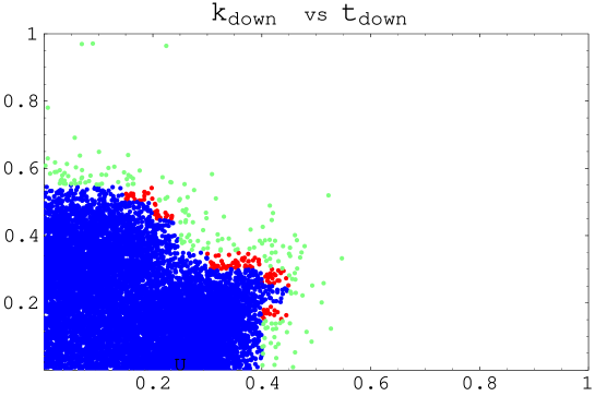
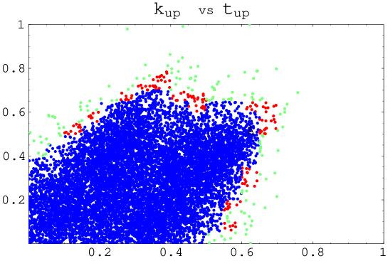
Figures 1 and 2 show the density of points in the planes $k_{d}$  vs $t_{d}$ and  $k_{u}$  vs $t_{u}.$ Points are blue (black) in regions where $R>0.1$ and green (light gray) where $R<0.05$.
A large fraction of the $t$ and $k$ space is essentially forbidden. We can put an upper bound to all the exponents. Namely, $t_{d}\lesssim 0.55$, $k_{d}\lesssim 0.4$ $t_{u}\lesssim 0.7$, $k_{d}\lesssim 0.65$. This is expected since large values for $t_{u,d}$ and $k_{u,d}$ increase the off-diagonal elements in the CKM matrix, in contrast with the experimental observation. The model previously mentioned [18, 19], prescribing eq. (23), lives on the border between the highly populated and the empty regions: in the up sector (fig.2) a slightly higher $t_{u}$ would fall in the not populated region. Similar conclusions, but in the down sector (fig. 1), apply for the model [20], with exponents given in equation (24). In these specific models, a closer study of the evolution of the Yukawa couplings (through the renormalization group equations) from the unification scale down to the weak scale could be desirable if one wishes a more definite conclusion.
One should also note that, even if the experiments put strong bounds on the CKM parameters,  the allowed regions for $t_{u,d}$ and $k_{u,d}$ are quite large; we have verified that a reduction on the errors of the $\bar{\rho}$ and $\bar{\eta}$  parameters would have a negligible impact on Figures 1 and 2. We conclude that errors coming from the  theoretical uncertainties (25) are dominant.

For the moment, a large range of possibilities exists: even a scenario with all exponents set to zero $t_{u,d}=k_{u,d}=0$ like in the following mass matrices gives acceptable predictions.

$$\ \ M_{u}\propto\left(\begin{tabular}[]{ccc}$u$&$u$&$u$\\ $c$&$c$&$c$\\ $1$&$1$&$1$\end{tabular}\right)$$

(27)

3.2 U(2) horizontal symmetry

Another class of models is based on a $U(2)$ horizontal symmetry. This symmetry acts on the known fermion families as follows. The light quarks transform as doublets ${\bf 2}$ under the $U(2)$ group

$$\matrix{{\bf 2}=\pmatrix{u_{L}\cr c_{L}\cr}&\pmatrix{u_{R}^{c}\cr c_{R}^{c}\cr}&\pmatrix{d_{L}\cr s_{L}\cr}&\pmatrix{d_{R}^{c}\cr s_{R}^{c}\cr}}.$$ (28)

$f_{L}$ are the lefthanded $SU(2)_{weak}$ doublets, while $f_{R}^{c}$ are the charge conjugated of the righthanded $SU(2)_{weak}$ singlets. The light Higgses (responsible for the electroweak breaking) are singlets as well as the quarks of the third generation. The $U(2)$ (differently from $SU(2)$) includes a $U(1)$ phase transformation: the ${\bf 2}$ and the ${\bf\bar{2}}$ are not equivalent representations; in particular such a $U(2)$ forbids Yukawa interactions like [24, 22]

$${\rm\ }g_{u}H_{u}\;\overline{u}_{L}u_{R}+g_{c}{\rm\ }H_{u}\;\overline{c}_{L}c_{R}$$ (29)

as well as all possible mass or mixing terms concerning the two lightest generations. On the contrary the top and bottom quarks can have mass since they are singlets under the above $U(2).$ To allow the lighter fermions acquiring a mass, we need to break the $U(2)$ symmetry in two steps. Firstly, the breaking of $U(2)\rightarrow U(1)$ can be induced by a $U(2)$-doublet $\phi_{a}$, the ${\bf 2}$, and a triplet $\Phi_{ab}$, the ${\bf 3}$. Exploiting the $U(2)$ symmetry we can always rotate their $vev$’s in order to obtain $\langle\phi_{2}\rangle=v_{1}$, $\langle\Phi_{22}\rangle=v_{2}$ and $\langle\phi_{1}\rangle=\langle\Phi_{11}\rangle=\langle\Phi_{12}\rangle=\langle\Phi_{21}\rangle=0$ which implies the following Yukawa couplings

$${\rm\ }gH_{u}\;\overline{c}_{L}t_{R}\;\phi_{2}+g^{\prime}{\rm\ }H_{u}\;\overline{c}_{R}t_{L}\;\phi_{2}^{\ast}+g^{\prime\prime}{\rm\ }H_{u}\;\overline{c}_{L}c_{R}\;\Phi_{22}+{\rm h.c.}$$ (30)

or in terms of the quark mass matrix

$$M_{up}\propto 1/M\;\pmatrix{0&0&0\cr 0&v_{2}&v_{1}\cr 0&v_{1}&M_{u}}.$$ (31)

An analogous matrix arises for the down sector. At lower energy also the $U(1)$ can be broken by a $U(2)$-singlet $A_{ab}$, antisymmetric under the exchange of the indices $a$ and $b$. This changes the matrix (31) into

$$M=\pmatrix{0&-v_{3}&0\cr v_{3}&v_{2}&v_{1}\cr 0&v_{1}&M_{u}}$$ (32)

where the scale of the $U(1)$ symmetry breaking is much smaller than the $U(2)$ symmetry breaking, i.e. $v_{3}\ll v_{1}\simeq v_{2}$. The zeros in the entries

$$M_{13}=M_{31}=M_{11}=0$$ (33)

are a generic consequence of this class of models: we will exploit the conditions (33) to parameterize the quark mass matrices (we make no assumption on the other entries); starting from the texture (33), we will considerably simplify the problem of extracting all mass hierarchies from the data; and at the same time, this will leave us with a reasonably large and assorted selection of models. To be more concrete, after the conditions (33) we are left with 6+6 non-zero entries that can be parametrized by 12 free complex variables as follows (to simplify the notation, we omit the up/down subscript in the exponents)

$$M_{up}=M_{u}\pmatrix{0&a_{1}^{u}\epsilon_{1}^{1-p_{u}}&0\cr a_{2}^{u}\epsilon_{1}^{p_{u}}&a_{3}^{u}\epsilon_{2}&a_{4}^{u}\epsilon_{2}^{r_{u}}\cr 0&a_{5}^{u}\epsilon_{2}^{d_{u}}&a_{6}^{u}},$$ (34)

and

$$M_{down}=M_{d}\pmatrix{0&a_{1}^{d}\epsilon_{3}^{1-p_{d}}&0\cr a_{2}^{d}\epsilon_{3}^{p_{d}}&a_{3}^{d}\epsilon_{4}&a_{4}^{d}\epsilon_{4}^{r_{d}}\cr 0&a_{5}^{d}\epsilon_{4}^{d_{d}}&a_{6}^{d}}.$$ (35)

Clearly one could choose a different reasonable parameterization with different parameters: nevertheless the needed 12 parameters would be in one to one correspondence with ours (shown in (34,35)) through well defined equations. Thus we do not loose in generality, choosing the above parameterization, here the only assumption is equation (33). The determinant of (34) gives the product of the three eigenvalues and thus $m_{up}m_{charm}m_{top}\sim\epsilon_{1}M_{u}^{3}.$ We also observe that $M_{u}\sim m_{top}$, and $\epsilon_{2}\sim m_{charm}/m_{top{\rm\ }}$(if $r+d\gtrsim 1$), then we also get that $\epsilon_{1}\sim m_{up}m_{charm}/m_{top}^{2}.$ A similar estimate holds for the down sector, where $\epsilon_{3}$ and $\epsilon_{4}$  are related to the down quark masses. The exponents $p_{u,d},r_{u,d},d_{u,d}$ need a more complex analysis that will be done in the next section.

The coefficients $a_{i}^{u,d}$ take into account the intrinsic theoretical uncertainties due to unknown fundamental parameters of the high energy physics. They are expected to be of order one : $|a_{i}^{u,d}|\simeq 1$ with $0<{\rm\arg}(a_{i}^{u,d})<2\pi$.

The $U(2)$ symmetry breaking, naively discussed above, implies definite values for the exponents

$$\begin{array}[]{ccc}p_{u}=1/2,&r_{u}=1,&d_{u}=1\\ p_{d}=1/2,&r_{d}=1,&d_{d}=1;\end{array}$$ (36)

however a more sophisticated theoretical study could lead to different scenarios, as for instance if one embeds the above picture into Grand Unified Theories. Our aim is to extract these exponents directly from the experimentally measured quantities, in the same line as shown in section (3.1). Before moving to this determination, we would like to show with an example the importance of the precise determination of the $\overline{\rho}$ and $\overline{\eta}$ parameters in excluding the above solution (36) for the exponents.

3.3 Importance of the precise determination of $\overline{\rho}$ and $\overline{\eta}$ parameters

In this example we use the values for the exponents that correspond to the U(2) symmetry breaking given in equation (36). This choice implies that [21, 24, 23] :

$$\begin{array}[]{ccc}\frac{V_{ub}}{V_{cb}}&=&\sqrt{\frac{{m_{u}}}{{m_{c}}}}\\ \frac{V_{td}}{V_{ts}}&=&\sqrt{\frac{{m_{d}}}{{m_{s}}}}\end{array}$$ (37)

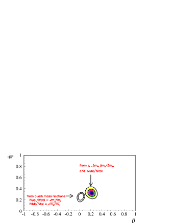
These relations are not exact due to the presence of the order-1 coefficients. On the other hand, as discussed in [24], the larger correction is on the first relation in (37) and is of order 10$\%$. Equation (37) can be used to define an allowed region in the ($\overline{\rho}$-$\overline{\eta}$) plane as shown in Figure (3). This region has been obtained by adding an extra 10$\%$ random correction to the first equation in (37) to take into account the above-mentioned effect [24]. In this Figure the $\overline{\rho}$-$\overline{\eta}$ allowed region is compared with the one selected by the measurements of $\left|\varepsilon_{K}\right|$, $\left|{\rm V}_{ub}/{\rm V}_{cb}\right|$, $\Delta m_{d}$ and from the limit on $\Delta m_{s}$. The two selected regions are far to be compatible (to be more quantitative see next paragraph). The significant improvement in the determination of the $\overline{\rho}$ and $\overline{\eta}$ parameters, obtained recently, allows to draw clear conclusions on the U(2) horizontal symmetries. As it was anticipated in [24] the high limit on the $B_{s}$-$\bar{B_{s}}$ mixing parameter, $\Delta m_{s}$, disfavours the naive U(2) symmetry breaking.

Figure 3: The allowed region for $\overline{\rho}$ and $\overline{\eta}$ (the contours at 68 $\%$ and 95 $\%$ probability are shown). Coloured contours : regions obtained using the constraints given by the measurements of $\left|V_{ub}\right|/\left|V_{cb}\right|$, $\left|\varepsilon_{K}\right|$, $\Delta m_{d}$ and $\Delta m_{s}$. Empty contours : regions obtained using the relation given in equation (37).

In the next section we extract the exponents of a generic U(2) horizontal symmetry directly from the experimentally measured quantities.

3.4 Fitting the mass hierarchies in the horizontal U(2) models

Figure 4: U(2) Horizontal Symmetries. The exponent $p_{d}$ (vertical axis) vs $p_{u}$. The letter “ U” marks the naive $U(2)$ prediction discussed in the text.

Figure 5: U(2) Horizontal Symmetries. The exponent $r_{d}$ (vertical axis) vs $r_{u}$

Figure 6: U(2) Horizontal Symmetries. The exponent $d_{d}$ (vertical axis) vs $p_{d}$. The letter “ U” marks the naive $U(2)$ prediction discussed in the text.

Figure 7: U(2) Horizontal Symmetries. The exponent $d_{d}$ (vertical axis) vs $p_{u}$

The $a^{u,d}\simeq 1$ coefficients in eq. (34,35) (differently from the Abelian case) are redundant: for example, if $|a_{4}^{u}|\neq 1$, one can reabsorb the norm $|a_{4}^{u}|$ in eq. (34) into a redefinition of $r_{u}\rightarrow r_{u}+\log|a_{4}^{u}|/\log\epsilon_{2}$ of the exponent $r_{u}$; thus one could set $|a_{i}^{u,d}|=1$ without loosing in generality.

Namely, we have assigned a flat probability to all the coefficients $a_{i}^{u,d}$ with

$$\matrix{|a_{i}^{u,d}|=1,&0<{\mathrm{arg}}(a_{i}^{u,d})<2\pi,\cr&\cr 0<t_{u,d}<1&0<d_{u,d},r_{u,d}<5}$$ (38)

As in the Abelian case, the range of variation of $t_{u,d}$ is fixed by the requirement that the entries (1,2) and (2,1) are smaller than the entry (3,3) in matrices (34,35). $d_{u,d}$ and $r_{u,d}$ could go from zero to infinity, but we have checked (see after) that for values greater than five the corresponding entries were absolutely negligible. In practice, the case $r_{u,d}>5$ (or $d_{u,d}>5$) is equivalent to $r_{u,d}=5$ (or $d_{u,d}=5$).

For any random choice of the coefficients $a_{i}^{u,d}$, of the exponents $p_{u,d},~{}r_{u,d},~{}d_{u,d}$ and the $vev$ $\epsilon$’s we get six physical quark masses and the CKM matrix. The large statistical sample of collected events has been compared with the experimental data (see section 2) and a weight defined for each event, corresponding to the probability distribution (26) . We have found that the overall probability distribution is maximal in regions shown in Table 3, even if it is still high and acceptable in a larger domain.

$p_{u}$ $\sim 0.33$ $d_{u}$ $\gtrsim 0.3$ $r_{u}$ $\sim 0.5$ $\ \ p_{d}$ $\sim 0.5$ $d_{d}$ $\sim 0.15\div 0.35$ $r_{d}$ $>1$	$p_{u}$ $\sim 0.33$ $d_{u}$ $\gtrsim 0$ $r_{u}$ $\gtrsim 1.$ $\ \ p_{d}$ $\sim 0.5$ $d_{d}$ $\sim 0.15\div 0.35$ $r_{d}$ $\sim 1$
$p_{u}$ $\sim 0.52$ $d_{u}$ $\gtrsim 0.5$ $r_{u}$ $\sim 0.5$ $\ \ p_{d}$ $\sim 0.48$ $d_{d}$ $0.6\div 1.2$ $r_{d}$ $>1$	$p_{u}$ $\sim 0.52$ $d_{u}$ $\gtrsim 0.3$ $r_{u}$ $\gtrsim 1$ $\ \ p_{d}$ $\sim 0.48$ $d_{d}$ $0.6\div 0.9$ $r_{d}$ $0.6\div 0.9$

Table 3: Four regions in the space of the exponents $p_{u,d},~{}r_{u,d},~{}d_{u,d}$ that maximize the probability distribution.

The two solutions on top of Table 3, prefer asymmetric quark mass matrices: $p_{u}\sim 0.33$ implies that the entry $(1,2)$ (in the up sector) is roughly the square of the entry $(2,1)$; also $d_{d}<r_{d}$ gives an entry (3,2) much larger than the (2,3) (in the down sector).

The remaining two solutions (bottom row of Table 3) appears more symmetric: a slight asymmetry is due to the exponents $p_{u}=0.52$ and $p_{d}=0.48$. But these are very close to 1/2, thus giving approximately symmetric matrices.

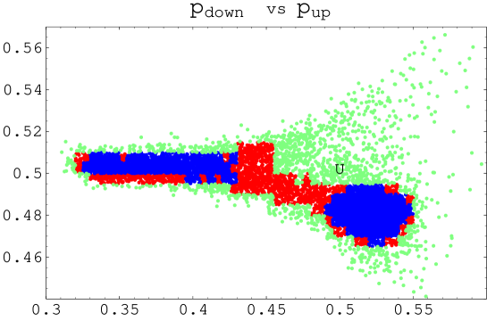
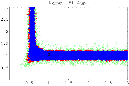
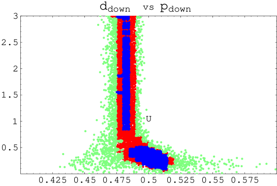
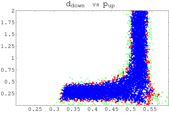
The six exponents show a significant statistical correlation; unfortunately we can only project the sample of events on two dimensional plots, thus in Figures 4-7, the number of points per unit area tells us the probability distribution as function of  each pair  of the variables $p_{u,d},~{}r_{u,d},~{}d_{u,d}$ (while the remaining four variables are integrated out); In the Figures , points are blue (black) in regions where $R>0.1$, red (gray) in regions where $0.05<R<0.1$, and green (light gray) where $R<0.05$. In Figure 4 we see the points distribution in the plane $p_{d}$ vs $p_{u}$. Note that the allowed region is small, in particular $p_{d}$ is very well determined and $R>0.05$ only if $0.46\lesssim p_{d}\lesssim 0.51$. The exponent in the down sector $p_{d}$ is better measured than the up one, and its value is close to $1/2$ which yields the well known relation

$$\sqrt{m_{d}/m_{s}}\simeq\sin\theta_{c}.$$ (39)

The parameterization for the up and the down sector are completely equivalent but experimental data prefer to constrain the down sector, while $p_{u}$ can vary from 0.32 to 0.55. With U we have marked the special case of a naive $U(2)$ symmetry as in (36).
In Figure 5 $r_{d}$ and $\ r_{u}$ are strongly correlated: either $r_{d}\sim 1$  or $r_{u}\sim 0.5.$   In fact if $r_{d}\sim 1$  and $r_{u}\gg 0.5$ one would have $V_{cb}\sim m_{s}/m_{b}$; instead $r_{u}\sim 0.5$  and  $r_{d}\gg 1$ yield $V_{cb}\sim\sqrt{m_{c}/m_{t}}.$ Both are possible and at least one of them must hold. In Figure 6 ($d_{d}$ vs $p_{d}$)  one clearly sees that the point U (referring to the model (36)) is outside the populated region. One can overcome this problem decreasing $d_{d}$ towards the region with maximal density $d_{d}\lesssim 0.5.$  Note, however, that $r_{d}\gtrsim 1$ (fig.5) and $d_{d}\lesssim 0.5$ imply  [23] an asymmetric down quark matrix  (35). In addition, decreasing $d_{d}$  one also pushes $p_{d}$ very close to 0.5, and (from Figure 4) this solution slightly prefers $p_{u}\lesssim 0.4,$ that is the region with maximal density, as also shown in Table 3. Also Figure 7 put in evidence a similar behavior: $\ p_{u}$ can easily range from 0.32 to 0.55, for low values of $d_{d}$; instead points with $d_{d}\gtrsim 0.5$ live in a much more restricted area  with $0.5\lesssim p_{u}\lesssim 0.55.$   Before concluding this section it is worthwhile to note that our approach can be used to test if a zero entry is favoured or disfavoured by data. For example, in Figure 6  one can see that for $d_{d}\gtrsim 1$  the shape of the point distribution no longer depends from $d_{d}$ and remains constant  even for $d_{d}$ going to infinity. This clearly indicates that when the entry $M_{32}=\epsilon_{4}^{d}$  becomes negligible (i.e. zero) few acceptable models still survive, thus $M^{{\rm d}own}_{32}=0$ is not excluded by data (provided that $p_{d}$ is slightly reduced).

4 Conclusions

The aim of particle physics is to describe all existing phenomena with the smallest number of free parameters. In fact one usually expects that a deeper understanding of the foundations of the theory automatically implies a reduction of the number of free parameters. For the same reason, but in  a different context, we await for grand unification of forces, which replaces three gauge couplings with just one gauge coupling of the embedding (simple) group.

Differently from the electroweak boson masses, in the fermion sector there are several free parameters. Understanding their origin in terms of new broken symmetries is difficult because the number of measurements is much less than the number of such parameters. The consequent ambiguity in extracting the eighteen complex entries of the quark mass matrices makes very difficult to disentangle the true underlying (broken) symmetry of the fermion sector. An approximate analytical approach,  like those based on estimates of the observables in terms of powers of the Cabibbo angle, can become inaccurate when several physical observables are involved: if  a fine tuning of the coefficients $a$’s of order 1/3 is required  to get the right $V_{cb}$ , one can safely conclude that the model is acceptable; but  if this tuning has to be repeated for  each observable,  the model becomes unacceptable. We have concluded that a global analysis based on a Monte Carlo  procedure with model independent parameterizations can give us more clear and trustable conclusions. We have shown how such an approach can be successfully implemented, achieving more information with less theoretical prejudice.  The progress brought by this Bayesian approach is the fact that we can put some confidence levels to some important parameters which otherwise would be unknown.We can test how precise are the determinations of the different exponents, and this makes clear to model builders which one of the theoretical ingredients is essential and which is not.

In case of Abelian symmetries we have found that the exponents $t$ and $k$ are poorly constrained. Still, an upper bound can be given to the four exponents: $t_{{\rm d}}\lesssim 0.55$, $k_{{\rm d}}\lesssim 0.4$ $t_{{\rm u}}\lesssim 0.7$, $k_{{\rm d}}\lesssim 0.65$. On the contrary, no lower bound arises from our analysis. The models explicitly discussed in the text lie in the highly populated region, even if near its boundary.

In the non Abelian scenario, namely when we (only) assume the (1,1), (1,3) and (3,1) entries to be zero, much stronger constraints can be set; also strong correlations between exponents of the down and up sectors arise. The naive $U(2)$ predictions appear ruled out. Instead, two alternative scenarios are suggested by current data: one where $d_{{\rm d}}$ is preferably around $0.25$. This value contradicts the naive $U(2)$ prediction $d_{{\rm d}}=1$. At the same time $r_{{\rm d}}\gtrsim 1,$ and  that requires an asymmetric texture $M_{32}^{{\rm d}}\gg M_{23}^{{\rm d}}$. This agrees with the analysis [23] . Such large $M_{32}^{{\rm d}}$ , in GUT theories [26],  implies a large (2,3) entry in the neutrino Dirac mass which, in turn, favours a large mixing in the atmospheric neutrinos [20, 23, 25].

A second scenario allows us to keep the same hierachies as in the naive $U(2)$ , but with   a slight (left-right) asymmetry in the (1,2) (2,1) entries (both in the up sector and in the down sector).  Namely $|M_{12}^{{\rm u}}|\sim 2|M_{21}^{{\rm u}}|$ and $|M_{12}^{{\rm d}}|\sim 0.7|M_{21}^{{\rm d}}|$ .

References

- [1] M. E. Peskin and D. V. Schroeder, “An Introduction To Quantum Field Theory,” Reading, USA: Addison-Wesley (1995) 842 p.
- [2] G. Altarelli, F. Caravaglios, G. F. Giudice, P. Gambino and G. Ridolfi, JHEP 0106 (2001) 018
- [3] H. Fusaoka and Y. Koide, Phys. Rev. D57 (1998) 3986.
-
[4]
F. Abe et al., CDF Collaboration, Phys. Rev. Lett.
74 (1995) 2626;
S. Abachi et al., D0 Collaboration, Phys. Rev. Lett. 74 (1995) 2632. - [5] V. Gimenez, L. Giusti, G. Martinelli, F. Rapuano, JHEP 0003:018,2000; D. Becirevic, V. Lubicz, G. Martinelli, Phys.Lett.B524:115-122,2002; J. Rolf, S. Sint, Nucl.Phys.Proc.Suppl.106:239-241,2002.
- [6] M.B. Voloshin, Int. J. Mod. Phys. A10 (1995) 2865; hep-ph/9502224.
- [7] A.H. Hoang, CERN-TH-2000-227; hep-ph/0008102.
- [8] J.H. Kühn and M. Steinhauser, hep-ph/0109084.
- [9] M. Eidemuller and M. Jamin, QCD 00, Montpellier, France, 6-13 Jul 2000; Nucl. Phys. Proc. Suppl. 96 (2001) 404.
- [10] S. Chen, M. Davier, E. Gámiz, A. Höcker, A. Pich and F. Prades, hep-ph/0105253.
- [11] J. G. Körner, F. Krajewski and A. A. Pivovarov, Eur. Phys. J. C20 (2001) 259.
- [12] H. Leutwyler, Phys. Lett. B378 (1996) 313.
- [13] G. Amoros, J. Bijnens and P. Talavera, Nucl. Phys. B602 (2001) 87.
- [14] L. Wolfenstein, Phys. Rev. Lett. 51 (1983) 1945.
- [15] M. Ciuchini, G. D’Agostini, E. Franco, V. Lubicz, G. Martinelli, F. Parodi, P. Roudeau and A. Stocchi, JHEP 0107 (2001) 013; hep-ph/0012308.
- [16] L. E. Ibanez and G. G. Ross, Phys. Lett. B 332 (1994) 100.
- [17] E. Dudas, C. Grojean, S. Pokorski and C. A. Savoy, Nucl. Phys. B 481 (1996) 85.
- [18] P.Binetruy and P.Ramond, Phys. Lett. B 350 (1995) 49; P. Binetruy, S. Lavignac and P. Ramond, Nucl. Phys. B 477 (1996) 353.
- [19] N. Irges, S. Lavignac and P. Ramond, Phys. Rev. D 58 (1998) 035.
- [20] G. Altarelli, F. Feruglio and I. Masina, JHEP 0011 (2000) 040
- [21] P.Ramond, R.G. Roberts and G.G. Ross , Nucl. Phys. B406 (1993) 19; L.J. Hall and A. Rasin, Phys. Lett. B315 (1993) 164; H. Fritzsch, Nucl. Phys. B155 (1979) 189; R. Gatto, G. Sartori and M. Tonin, Phys. Lett. B28 (1968) 128; R.J. Oakes, Phys. Lett. B29 (1969) 683 [Erratum B31(1970) 630]; Phys. Lett. B30 (1970) 26.
- [22] K. S. Babu and R. N. Mohapatra, Phys. Rev. Lett. 83 (1999) 2522.
- [23] R. G. Roberts, A. Romanino, G. G. Ross and L. Velasco-Sevilla, Nucl. Phys. B 615 (2001) 358; A. Masiero, M. Piai, A. Romanino and L. Silvestrini, Phys. Rev. D 64 (2001) 075005.
- [24] R. Barbieri, L. J. Hall and A. Romanino, Nucl. Phys. B551 (1999) 93 and references therein.
- [25] Z. Berezhiani and A. Rossi, JHEP 9903 (1999) 002.
- [26] G. Anderson, S. Raby, S. Dimopoulos, L. J. Hall and G. D. Starkman, Phys. Rev. D 49 (1994) 3660.