Scanning of the $e^{+}e^{-}\rightarrow\pi^{+}\pi^{-}$ cross–section below 1 GeV by radiative events with untagged photon

Abstract

We discuss an inclusive approach to the measurement of the $e^{+}e^{-}\rightarrow\pi^{+}\pi^{-}$ cross–section by the radiative return method without photon tagging. The essential part of this approach is the choice of rules for event selection which provide rejection of events with 3 (or more) pions and decrease the final–state radiation background. The radiative corrections to the initial–state radiation process are computed for DA$\Phi$NE conditions, using the quasi–real electron approximation for both, the cross–section and the underlying kinematics. The two cases of restricted and unrestricted pion phase space are considered. Some numerical calculations illustrate our analytical results.

¹ Department of Physics and Institute for Particle Physics Phenomenology, University of Durham, DH1 3LE, UK and Petersburg Nuclear Physics Institute, Gatchina, 188350, Russia

² National Science Centre Kharkov Institute of Physics and Technology, 61108 Akademicheskaya 1, Kharkov, Ukraine

³ INFN Laboratori Nazionali di Frascati, P.O. Box 13, 00044 Frascati, Italy

⁴ Dipartimento di Fisica, Universita’ di Parma and INFN, Gruppo Collegato di Parma, 43100 Parma, Italy

PACS: 12.20.-m, 13.40.-f, 13.60.-Hb,

13.88.+e

1 Introduction

The recent high precision measurement of the muon anomalous magnetic moment $(g-2)_{\mu}$ [1] has boosted interest in renewed theoretical calculations of this quantity [2], since any difference between the experimental value and the theoretical evaluations based on the Standard Model (SM) may open a window into possible new physics [3]. While conclusions about posssible discrepancy with the SM are premature [4], the Brookhaven based experiment is now planning a new measurement with three times better accuracy, which may create further challenges to the theory. Presently, there are two main sources of theoretical uncertainty in the calculation, namely the impact of the light-by-light contribution [5, 6, 7] and the estimate of the error from the hadronic vacuum polarization contribution to $(g-2)_{\mu}$. In this paper we address the question of this error, for which different groups give different results [8, 9].

The problem of the hadronic vacuum polarization contribution is that it cannot be calculated analytically because perturbative QCD loses its predictive power at low and intermediate energies, where, on the other hand, the effect is the largest. However one can evaluate this hadronic term from the data on electron-positron annihilation into hadrons by using a dispersion relation [10]. The necessary condition for a theoretical error matching the experimental accuracy reached in the $(g-2)_{\mu}$ measurement, is the knowledge of the total hadronic cross section with better than one per cent accuracy. The recent precision measurements of the total hadronic cross-section by the CMD-2 [11] and BESII [12] collaborations were included in the new analysis of Refs. [13, 14]. While this reduces the error in the hadronic contribution to the shift in the running electromagnetic coupling, for the muon (g-2) value it is mandatory to perform new measurements of the total cross section at energies below 1.4 GeV (in particular, in the $e^{+}e^{-}\rightarrow\pi^{+}\pi^{-}$- channel) with at least one per cent accuracy. Such accurate measurement will then be important not just for the muon anomalous magnetic moment but also for testing the effective fine structure constant.

In the last years, the idea to use radiative events in electron-positron collisions for scanning of the total hadronic cross section has become quite attractive. The radiative return approach was first discussed long ago, and the lowest-order cross sections for the radiative process of electron-positron annihilation into a pair of charged fermions or scalar bosons were calculated [15]. This subject was subsequently studied in several papers (see, for example, [16, 17, 18, 19, 20]), where higher-order radiative corrections were taken into account.

Due to differences in the systematic uncertainties in the measurement, the radiative return approach has several advantages when compared to the conventional energy scan : for example, luminosity and beam energy effects are accounted for only once. For variable total hadronic energies from the $2m_{\pi}$ threshold up to 1.02 GeV, the ideal machine for scanning the total cross section, using the radiative return method, appears to be the DA$\Phi$NE accelerator, operating at the $\Phi$ resonance, together with the KLOE detector[18, 21, 22]. DA$\Phi$NE measurements can become quite competitive to the conventional direct cross section scan, and, as mentioned, have certain advantages due to the systematics. The radiative return method allows to perform precise measurements of the hadronic cross sections in the $\rho$ resonance region. The high accuracy of scanning is provided by the high resolution measurement of the pion 3-momenta (and consequently the invariant mass) with the KLOE drift chamber. Recently the first preliminary results of such measurements of $\pi^{+}\pi^{-}$ production cross section below 1 GeV have been reported [22].

In our previous paper [20] the analysis of Initial State Radiation (ISR) effects, which provide the basis for the radiative return strategy, has been performed for the realistic conditions of the KLOE detector. It was assumed that both the energy of the photon in the calorimeter, and the invariant mass of the $\pi^{+}\pi^{-}$ - system were measured.

Notice that the KLOE detector allows to register photons only outside two narrow cones along the beam directions (the so-called blind zones ). Because of this geometrical restriction, most of the ISR events become inaccessible for tagging and cannot be recorded by the photon detector. This decreases the statistics and, thus, results in lesser precision. In order to avoid this problem and, moreover, to fully exploit the possibility of high precision measurement of the two charged pions with the drift chamber [18, 21], it was proposed to make the photon tagging redundant. The idea is to use an Inclusive Event Selection (IES) approach, in which only the invariant mass of the final pions is measured, and the ISR photon remains untagged.

As briefly discussed in [20], one of the main advantages of the IES strategy is the rise of the corresponding cross section caused by the $\ln(E^{2}/m^{2})$ enhancement (here $E$ is the beam energy and $m$ is the electron mass) due to the possibility to include events with ISR collinear photons which, otherwise, belong to the blind zones. As shown in [23], the number of such untagged photon events exceeds by about a factor three the number of events with the tagged photon (if the opening angle of the blind zone equals to $10^{o}$).

Of course, in order to avoid uncertainties in the interpretation of IES approach and to have the possibility to describe IES in terms of ISR events, some additional event selection criteria should be imposed. The corresponding additional restrictions should make the photon tagging redundant, but at the same time should guarantee the suppression of the main background caused by events from $\Phi\rightarrow\pi^{+}\pi^{-}\pi^{0}$ decay.

In this paper we present the analytical calculation of the Born cross section of ISR process

$$e^{-}(p_{1})+e^{+}(p_{2})\rightarrow\gamma(k)+\pi^{+}(p_{+})+\pi^{-}(p_{-})$$ (1)

and the QED radiative corrections (RC) to it for IES setup, accounting for the additional kinematical constraints on the event selection, which can be realized at KLOE. The physics motivation for these constraints is discussed in Section 2.

The Born IES cross section is calculated in Section 3. Note that for a chosen set of selection rules, IES cross section at the Born level coincides with the tagged photon events cross section as given in Ref. [16], provided that the final pion phase space is unrestricted. But we consider also the realistic case when the pion phase space is restricted.

In Section 4 we discuss the RC to the Born cross section caused by the emission of real and virtual photons. At the RC level, the IES cross section differs from the tagged photon result because of the contribution of double photon bremsstrahlung. The situation here is similar to the case of radiative corrections in DIS with detected lepton (the analogue of the tagged photon events) or hadrons (analogous to the IES). In the latter case, the radiative corrections factorize while in the former they include by necessity some integrals over hadronic cross section that have to be extracted from experimental data. This fact certainly makes the IES approach more advantageous. In Section 5 the cancellation of the infrared and collinear parameters, used in the calculations of radiative corrections, is demonstrated, and the expression for the total photonic contribution to the radiative corrections is given. In Section 6 we discuss also possible contribution of the $e^{+}e^{-}$–pair production into the IES cross section if the $e^{+}e^{-}\pi^{+}\pi^{-}$ final state is not rejected by the analysis procedure. Our Conclusion contains a brief summary and the discussion of the background processes which may contribute into the IES cross section.

2 IES selection rules

As mentioned in the Introduction, the main condition of the IES approach is the precise measurement of the di–pion invariant mass in process (1). In addition, restrictions must be imposed in order to select final states with only $\pi^{+}\pi^{-}+n\gamma$ , excluding $\pi^{+}\pi^{-}\pi^{0}$. Finally, we have to add some constraints in order to reduce contributions from final state radiation (FSR). As an added bonus, such contraints also simplify the theoretical calculation of the radiative corrections.

Rejection of the 3–pion final state in process (1) can be done selecting events with an appropriately small difference between the lost (undetected) energy and the modulus of the lost 3–momentum in process (1). In terms of the measured pion 3–momenta, this restriction reads [18, 20, 21]

$$2E-E_{+}-E_{-}-|{\bf P}_{\Phi}-{\bf p_{+}-p_{-}}|<\eta E\ ,\ \ \eta\ll 1,$$ (2)

where $E$ is the beam energy, $E_{\pm}=\sqrt{{\bf p}_{\pm}^{2}-m_{\pi}^{2}}$ is the energy of $\pi^{\pm}$, and $m_{\pi}$ is the pion mass. ${\bf P}_{\Phi}$ is the total initial–state 3–momentum which, at DA$\Phi$NE, is non-zero, due to a small acollinearity in the beams, $|{\bf P}_{\Phi}|=12.5MeV.$ If the chosen parameter $\eta$ is small enough ($\leq(m_{\pi}/E)^{2})$, constraint (2) allows to avoid the undetected $\pi^{0}$ and to retain only the undetected $n\gamma$ system. Inequality (2) can be rewritten in terms of the total energy $\Omega$ and modulus of the total 3–momentum $|{\bf K}|$ of all photons in the reaction $e^{+}+e^{-}\rightarrow\pi^{+}+\pi^{-}+n\gamma$ as

$$\Omega-|{\bf K}|<\eta E.$$ (3)

The optimal value $\eta=0.02$ decreases also the FSR background [18].

The next constraint selects such events, where at $n=1$ the undetected photon is collinear with the emitting electron (or positron). The collinear events considered here are those in which the photon belongs to a narrow cone with opening angle $2\theta_{0}\ (\theta_{0}\ll 1)$ along the electron beam direction (the blind zone for the KLOE detector). This constraint reads

$${\bf Kp_{1}>|K|}Ec_{0},\ \ c_{0}=\cos{\theta_{0}}\ ,$$ (4)

where ${\bf p_{1}}$ is the 3–momentum of the electron and $\theta_{0}$ can be chosen to be $5^{o}\div 6^{o}$. Due to this constraint, the collinear photon radiated by the initial electron contributes to the observed IES cross section and induces a $\ln(E^{2}\theta_{0}^{2}/m^{2})$ enhancement, which, at DA$\Phi$NE, makes the IES cross section a few times larger than in the tagged photon case. Moreover, the collinear constraint provides the possibility to apply the well known quasi–real electron (QRE) method [24] to calculate radiative corrections. Even at the Born level, the difference between the exact result and the corresponding QRE approximation is negligible (see for details Section 3). Selection rules (2), (3) and (4) imply precise measurements of the pion 3–momentum that can be provided by the KLOE drift chamber.

Note also that in the Born approximation ($n=1$) inequality (3) is always satisfied, and, therefore, the selection rules (3) and (4) imply non–trivial consequences only through the contribution to the radiative corrections from two hard photon emission.

Because of the existence of the blind zones, the KLOE detector cannot provide the detection of the final $\pi^{+}$ and $\pi^{-}$ inside the full phase space, picking out events with pion polar angles in the region

$$\theta_{m}<\theta_{\pm}<\pi-\theta_{m}\ .$$ (5)

In principle, $\theta_{m}$ can be taken to be about $10^{o}$, but, as shown by the Monte Carlo calculations [17, 18], the choice of $\theta_{m}$ influences also the value of the FRS background. The optimal value of $\theta_{m}$ for DA$\Phi$NE conditions is $20^{o}.$ [18]

Usually, the restricted pion phase space can be taken into account by introducing an acceptance factor $A(\theta_{m}).$ The calculation of this factor is very simple for a nonradiative process, but for the ISR process, and the RC to its cross section, it is non–trivial. The analytical form of $A(\theta_{m})$ can be derived in the framework of QRE approximation. To illustrate the problem, in the following we perform calculations for both unrestricted and restricted pion phase space.

3 Born approximation

To lowest order in $\alpha,$ the differential cross section of process (1) can be written in terms of the leptonic $L_{\mu\nu}$ and hadronic $H_{\mu\nu}$ tensors as (see Ref. [15])

$$d\sigma^{B}=\frac{8\pi^{2}\alpha^{2}}{sq^{4}}L^{\gamma}_{\mu\nu}(p_{1},p_{2},k)H_{\mu\nu}\frac{\alpha}{4\pi^{2}}\frac{d^{3}k}{\omega}\frac{d^{3}p_{+}d^{3}p_{-}}{16\pi^{2}E_{+}E_{-}}\delta(q-p_{+}-p_{-})\ ,$$ (6)

where $\omega$ is the energy of photon, and the hadronic tensor is expressed via the pion electromagnetic form factor $F_{\pi}(q^{2})$ as follows

$$H_{\mu\nu}=-4|F_{\pi}(q^{2})|^{2}\tilde{p}_{-\mu}\tilde{p}_{-\nu}\ ,\ \ \tilde{p}_{-\mu}=p_{-\mu}-\frac{1}{2}q_{\mu}\ ,\ \ q=p_{1}+p_{2}-k=p_{+}+p_{-}\ .$$

The pion electromagnetic form factor defines the total cross section $\sigma(q^{2})$ of the process $e^{+}+e^{-}\rightarrow\pi^{+}+\pi^{-}$, by means of relation

$$|F_{\pi}(q^{2})|^{2}=\frac{3q^{2}\sigma(q^{2})}{\pi\alpha^{2}\zeta},\ \ \zeta=\Bigl{(}1-\frac{4m_{\pi}^{2}}{q^{2}}\Bigr{)}^{\frac{3}{2}}\ .$$ (7)

In the case of unrestricted (full) pion phase space, the integration of the hadronic tensor can be performed in invariant form [15]

$$\frac{1}{16\pi^{2}}\int H_{\mu\nu}\frac{d^{3}p_{+}d^{3}p_{-}}{E_{+}E_{-}}\delta(q-p_{+}-p_{-})=\frac{q^{4}}{8\pi^{2}\alpha^{2}}\sigma(q^{2})\tilde{g}_{\mu\nu},\ \ \tilde{g}_{\mu\nu}=g_{\mu\nu}-\frac{q_{\mu}q_{\nu}}{q^{2}}\ ,$$ (8)

whereas for the restricted case we have first to contract the tensors in Eq. (6) and then to integrate the result over the pion phase space.

The leptonic tensor on the right–hand side of Eq. (6) for the case of collinear ISR along the electron beam direction is well known [15, 25]

$$L^{\gamma}_{\mu\nu}(p_{1},p_{2},k)=\Bigl{[}\frac{(q^{2}-t_{1})^{2}+(q^{2}-t_{2})^{2}}{t_{1}t_{2}}-\frac{2m^{2}q^{2}}{t_{1}^{2}}\Bigr{]}\tilde{g}_{\mu\nu}+\frac{4q^{2}}{t_{1}t_{2}}\tilde{p}_{1\mu}\tilde{p}_{1\nu}+\Bigl{(}\frac{4q^{2}}{t_{1}t_{2}}-\frac{8m^{2}}{t_{1}^{2}}\Bigr{)}\tilde{p}_{2\mu}\tilde{p}_{2\nu},$$ (9)

where

$$\tilde{p}_{1,2\mu}=p_{1,2\mu}-\frac{p_{1,2}q}{q^{2}}q_{\mu}\ ,\ t_{1}=-2kp_{1},\ t_{2}=-2kp_{2},\ s=2p_{1}p_{2},\ q^{2}=s+t_{1}+t_{2},$$

and we neglect terms of the order $|m^{2}/t_{2}|$ which are always below the required accuracy. The contraction of the leptonic tensor with $\tilde{g}_{\mu\nu}$ that is necessary to use in the case of unrestricted pion phase space reads

$$L^{\gamma}_{\mu\nu}(p_{1},p_{2},k)\tilde{g}_{\mu\nu}=2F\ ,\ \ F=\frac{(q^{2}-t_{1})^{2}+(q^{2}-t_{2})^{2}}{t_{1}t_{2}}-\frac{2q^{2}m^{2}}{t_{1}^{2}}\ .$$ (10)

In the case of restricted phase space we have to use the following relation

$$L^{\gamma}_{\mu\nu}(p_{1},p_{2},k)H_{\mu\nu}=4q^{2}|F_{\pi}(q^{2})|^{2}R\ ,$$ (11)

$$R=-\frac{m_{\pi}^{2}}{q^{2}}F+\frac{q^{2}(\chi_{1}+\chi_{2})-\chi_{1}^{2}-\chi_{2}^{2}}{t_{1}t_{2}}-\frac{\chi_{1}}{t_{1}}-\frac{\chi_{2}}{t_{2}}+\frac{2m^{2}\chi_{2}}{t_{1}^{2}}\Bigl{(}\frac{\chi_{2}}{q^{2}}-1\Bigr{)}\ ,\ \ \chi_{1,2}=2p_{1,2}p_{-}\ .$$

Therefore, the differential cross section of the process (1) in the Born approximation can be written as

$$d\sigma^{B}_{F}=\sigma(q^{2})\frac{\alpha}{2\pi^{2}}F\frac{d^{3}k}{\omega}\ ,$$ (12)

$$d\sigma^{B}_{R}=\frac{3\sigma(q^{2})R}{s\zeta}\frac{\alpha}{4\pi^{2}}\frac{d^{3}k}{\omega}\frac{|{\bf p}_{-}|dE_{-}dc_{-}}{E_{+}}\frac{d\varphi_{-}}{2\pi}\delta(2E-\omega-E_{+}-E_{-})\ ,$$ (13)

where $c_{-}=\cos{\theta_{-}}$ and $\theta_{-},\ \varphi_{-}$ are polar and azimuthal angles of the negative pion respectively (we take Z axis along the ${\bf p_{1}}$ direction).

It seems at first sight that one can perform the trivial integration with respect to the azimuthal angle $\varphi_{-}$ on the right–hand side of Eq. (13) because the quantity $R$ does not contain any $\varphi_{-}$–depending term. But in the general case the pion energies $E_{+}$ and $E_{-}$ depend on $\varphi_{-}.$ Moreover, the upper limit of integration over $c_{-}$ for the ISR events with collinear photon along the electron beam direction is smaller than $c_{m}=\cos{\theta_{m}}$ and depends on $\varphi_{-}$ as well, i.e.

$$-c_{m}<c_{-}<c_{max}\ ,\ \ \ c_{max}<c_{m}\ ,$$ (14)

where $c_{max}$ must be determined from the 3–momentum conservation, provided that $c_{+}=\cos{\theta_{+}}=-c_{m}.$ Therefore, in the case of the restricted pion phase space, it is necessary to first integrate over $c_{-}$ and then over $\varphi_{-}$.

Let us now perform the integration with respect to the photon angular phase space on the right–hand side of Eq. (12). It is convenient to choose $X$ axis along the ${\bf P}_{\Phi}$ direction. In the laboratory frame

$$p_{1}=(E,0,0,|{\bf p_{1}}|)\ ,\ \ p_{2}=(E,|{\bf P}_{\Phi}|,0,-p_{2z})\ ,\ \ p_{2z}=E\bigl{(}1-\frac{{\bf P}_{\Phi}^{2}}{2E^{2}}\bigr{)}$$ (15)

and

$$t_{1}=-2\omega(E-|{\bf p_{1}}|\cos{\theta})\ ,\ \ t_{2}=-2\omega E\bigl{[}1+\bigl{(}1-\frac{{\bf P}_{\Phi}^{2}}{2E^{2}}\big{)}\cos{\theta}\bigr{]}+2\omega|{\bf P}_{\Phi}|\sin{\theta}\cos{\phi}\bigr{]}\ ,$$

$$s=4E^{2}-{\bf P}_{\Phi}^{2},\ \ q^{2}=4E^{2}-4E\omega-{\bf P}_{\Phi}^{2}\bigl{(}1-\frac{\omega}{E}\cos{\theta}\bigr{)}+2\omega|{\bf P}_{\Phi}|\sin{\theta}\cos{\phi}\ ,$$ (16)

where $\theta$ and $\phi$ are polar and azimuthal angles of the photon radiated in the initial state. Keeping terms of the order ${\bf P}_{\Phi}^{2}/E^{2}$ and $\theta_{0}^{2},$ we can use the following list of integrals

$$\int\frac{d\,O}{-t_{2}}=\frac{\pi\theta_{0}^{2}}{4\omega_{0}E}\ ,\ \int\frac{d\,O}{-t_{1}}=\frac{\pi}{\omega_{0}E}\Bigl{[}\Bigl{(}1-\frac{{\bf P}_{\Phi}^{2}}{4E^{2}}\Bigr{)}L_{0}-\frac{\theta_{0}^{2}}{12}\Bigr{]}\ ,\ \int\frac{d\,Om^{2}}{t_{1}^{2}}=\frac{\pi}{\omega_{0}^{2}}\Bigl{(}1-\frac{{\bf P}_{\Phi}^{2}}{2E^{2}}\Bigr{)}\ ,$$

$$\int\frac{d\,Ot_{2}}{t_{1}}=4\pi\Bigl{[}\Bigl{(}1-\frac{{\bf P}_{\Phi}^{2}}{4E^{2}}\Bigr{)}L_{0}-\frac{\theta_{0}^{2}}{3}\Bigr{]}\ ,\ \ \ \int\frac{d\,O}{t_{1}t_{2}}=\frac{\pi}{4\omega_{0}^{2}E^{2}}\Bigl{[}\Bigl{(}1-\frac{{\bf P}_{\Phi}^{2}}{4E^{2}}\Bigr{)}L_{0}+\frac{\theta_{0}^{2}}{6}\Bigr{]}\ ,$$ (17)

$$\omega_{0}=\frac{4E^{2}-q^{2}-{\bf P}_{\Phi}^{2}}{4E}\ ,\ \ L_{0}=\ln{\frac{E^{2}\theta_{0}^{2}}{m^{2}}}\ ,\ \ d\,O=d\cos{\theta}d\phi\ .$$

When evaluating these integrals we systematically neglected small terms of order ${\bf P}_{\Phi}^{2}\theta_{0}^{2}/E^{2}.$ Within such approximation we can use the substitution

$$|{\bf P}_{\Phi}|\sin{\theta}\cos{\phi}\rightarrow 0,\ \ \ {\bf P}_{\Phi}^{2}\cos{\theta}\rightarrow{\bf P}_{\Phi}^{2}\ ,$$ (18)

in the expressions for the invariants $t_{1}$ and $t_{2}$ in Eqs. (17). With the same accuracy we can write

$$\omega d\omega=\frac{\omega_{0}dq^{2}}{4E}\Bigl{(}1+\frac{{\bf P}_{\Phi}^{2}}{2E^{2}}\Bigr{)}\ .$$ (19)

Combining (12), (17) and (19), we arrive at the distribution over the pion squared invariant mass $q^{2}$, for unrestricted pion phase space

$$\frac{d\sigma^{{}^{B}}_{F}}{dq^{2}}=\frac{\sigma(q^{2})}{4E^{2}}\frac{\alpha}{2\pi}\Bigl{[}\Bigl{(}\frac{q^{4}}{8\omega_{0}E}+\frac{q^{2}}{2E^{2}}+\frac{\omega_{0}}{E}\Bigr{)}\Bigl{(}1+\frac{{\bf P}_{\Phi}^{2}}{4E^{2}}\Bigr{)}L_{0}-\frac{q^{2}}{2\omega_{0}E}+\frac{\theta_{0}^{2}}{6}\Bigl{(}\frac{q^{4}}{8\omega_{0}E}+\frac{q^{2}}{2E^{2}}-\frac{2\omega_{0}}{E}\Bigr{)}\Bigr{]}\ .$$ (20)

To guarantee only one per cent accuracy one can neglect terms proportional to ${\bf P}_{\Phi}^{2}/4E^{2}$ and $\theta_{0}^{2}/6$ in (20) because their contribution into the IES cross section is of the relative order $10^{-4}.$ Such procedure leads to the well known result corresponding to the QRE approximation [24]

$$\frac{d\sigma^{{}^{B}}_{F}}{dq^{2}}=\frac{\sigma(q^{2})}{4E^{2}}\frac{\alpha}{2\pi}P(z,L_{0})\ ,\ P(z,L_{0})=\frac{1+z^{2}}{1-z}L_{0}-\frac{2z}{1-z}\ ,\ z=\frac{q^{2}}{4E^{2}}\ .$$ (21)

Thus, the QRE approximation appears to be sufficient for a description of the IES cross section and corresponds to a one per cent precision even at the Born level.

Consider now the case of the restricted pion phase space. First, the $\delta$–function on the right–hand side of Eq. (13) has to be used to perform the integration with respect to $E_{-}.$ Then within chosen accuracy we obtain

$$\frac{|{\bf p}_{-}|d\,E_{-}}{E_{+}}\delta(2E-\omega-E_{+}-E_{-})=\frac{|{\bf p}_{-}|^{2}}{|{\bf p}_{-}|(2E-\omega)+E_{-}(\omega c_{\gamma_{-}}-|{\bf P}_{\Phi}|s_{-}\cos{\varphi_{-}})}\ ,$$ (22)

where

$$c_{\gamma_{-}}=\cos{\theta}c_{-}+\sin{\theta}s_{-}\cos{(\phi-\varphi_{-})}\ ,\ \ s_{-}=\sin{\theta_{-}}\ ,\ \ \omega=\omega_{0}\Bigl{(}1+\frac{{\bf P}_{\Phi}^{2}}{4E^{2}}\Bigr{)}\ .$$

Now let us express $E_{-}$ in terms of the photon energy $\omega$ and angles of the photon and negative pion, using the energy–momentum conservation. The result can be written in the following form

$$E_{-}=\frac{AB-C\sqrt{B^{2}-4m_{\pi}^{2}(A^{2}-C^{2})}}{2(A^{2}-C^{2})}\ ,\ \ A=2E-\omega,\ \ B=4E(E-\omega)-|{\bf P}_{\Phi}|^{2}\ ,$$ (23)

$$C=\omega c_{\gamma_{-}}-|{\bf P}_{\Phi}|s_{-}\cos{\varphi_{-}}\ .$$

To find the energy of the positive pion it is necessary to use the relation $2E-\omega=E_{+}+E_{-}.$ Having expressions for the pion energies, we can apply conservation of the Z–component of 3–momentum at $c_{+}=-c_{m}$

$$-|{\bf p}_{+}|c_{m}+|{\bf p}_{-}|c_{-}+\omega\cos{\theta}=0$$ (24)

to derive the upper limit $c_{max}$ of the variable $c_{-}.$ In Eq. (24) both $|{\bf p}_{-}|$ and $|{\bf p}_{+}|$ are functions of $\omega,\ c_{-},\ \cos{\theta}$ and $\cos{(\phi-\varphi_{-})}.$ Therefore, to reach the same accuracy as in Eq. (20) for the case of the restricted pion phase space, the differential distribution over the pion invariant mass squared has to be taken in the form

$$\frac{d\sigma^{{}^{B}}_{R}}{d\,q^{2}}=\frac{12\sigma(q^{2})}{4E^{2}\xi}\frac{\alpha}{2\pi}\frac{\omega_{0}}{E}\Bigl{(}1+\frac{{\bf P}_{\Phi}^{2}}{2E^{2}}\Bigr{)}\int\limits_{c_{0}}^{1}d\cos{\theta}\int\limits_{0}^{2\pi}\frac{d\phi}{2\pi}\int\limits_{0}^{2\pi}\frac{d\varphi_{-}}{2\pi}\int\limits_{-c_{m}}^{c_{max}}d\,c_{-}\frac{R|{\bf p}_{-}|^{2}}{A|{\bf p}_{-}|+CE_{-}}\ ,$$ (25)

where $c_{0}=\cos{\theta_{0}}$ and the quantities $A,\ C$ are defined in (23). The analytical integration on the right–hand side of Eq. (25) is not available and the task of integration can be left for numerical calculation.

The result is very much simplified if one neglects terms of the order $|{\bf P}_{\Phi}^{2}|/E^{2}$ and use the QRE approximation, assuming $\cos{\theta}=1$ in expressions (22), (23) and (24). This leads to the IES cross section

$$\frac{d\sigma^{{}^{B}}_{R}}{d\,q^{2}}=\frac{\sigma(q^{2})}{4E^{2}}\frac{\alpha}{2\pi}P(z,L_{0})A(z,c_{m})\ ,$$ (26)

where $z$ is defined in (21) and

$$A(z,c_{m})=\frac{12}{\zeta}\int\limits_{-c_{m}}^{c_{max}}d\,c_{-}U\frac{z[(1+z)K-(1-z)c_{-}]^{2}}{K[(1+z)^{2}-(1-z)^{2}c_{-}^{2}]^{2}}\ ,\ U=\frac{\chi_{1}}{4E^{2}}-\frac{\chi_{1}^{2}}{16E^{4}}-\frac{m_{\pi}^{2}}{4zE^{2}}$$ (27)

represents the acceptance factor (see the end of the previous Section) as it follows from the comparison between the IES cross sections (21) and (26). To write down $A(z,c_{m})$ the following notations were used:

$$K=\sqrt{1-\frac{\delta^{2}}{z^{2}}[(1+z)^{2}-(1-z)^{2}c_{-}^{2}]}\ ,\ \ \frac{\chi_{1}}{4E^{2}}=\frac{z[1+z-2Kc_{-}+(1-z)c_{-}^{2}]}{(1+z)^{2}-(1-z)^{2}c_{-}^{2}}\ ,\ \delta^{2}=\frac{m_{\pi}^{2}}{4E^{2}}\ ,$$

$$c_{max}(z,c_{m})=\frac{(1+z)g}{\sqrt{(z-(1-z)g)^{2}-(1+z)^{2}\delta^{2}}}\ ,\ g=\frac{zc_{m}[(1+z)K(c_{m})+(1-z)c_{m}]}{(1+z)^{2}-(1-z)^{2}c_{m}^{2}}-\frac{1-z}{2}\ .$$ (28)

At fixed values of $c_{m}$, the quantity $c_{max}$ depends on the squared pion invariant mass $q^{2}=4E^{2}z.$ If $z$ is small enough (this situation corresponds to the radiation of a very hard collinear photon with the energy fraction $(1-z)$ by the electron) $c_{max}$, as formally defined by (28), can approach $-c_{m}$ and became even smaller. Because selection rule (5) forbids any values of $c_{max}$ smaller than $c_{m},$ it is necessary to substitute the upper limit of integration on the right–hand side of Eq. (27) by $max[c_{max},\ -c_{m}].$ If not, the formal calculation in (27) leads to negative values for the acceptance factor at small $z,$ as one can see from from Fig. 1 for $c_{m}=\cos{20^{o}}$ and $z\approx 0.1$, while really it equals to zero at such $z$–values. Note that in the framework of the QRE approximation one can use also energy conservation for events with $\theta_{+}=\pi-\theta_{m}$

$$E(1+z)=E_{-}(c_{max})+E_{+}(c_{+}=-c_{m})$$

in order to obtain the analytical form of $c_{max}$ on the Born level.

If $c_{m}=1$, 3–momentum conservation in process (1) requires $c_{max}(z,1)=1$ as well. In this case

$$K(c_{m})=\sqrt{1-\frac{4\delta^{2}}{z}}\ ,\ \ g=\frac{(1+z)K(c_{m})-1+z}{4},$$

and it is easy to see that $c_{max}(z,c_{m})$, as given by (28), satisfies this requirement.

In principle, the acceptance factor $A(z,c_{m})$ may be computed analytically by means of Euler’s substitution on the right–hand side of Eq.(27)

$$c_{-}=\frac{t^{2}-a^{2}}{2t},\ \ K=\frac{\delta(1-z)(t^{2}+a^{2})}{2zt},\ \ dc_{-}=\frac{(t^{2}+a^{2})dt}{2t^{2}},\ \ a^{2}=\frac{z^{2}-\delta^{2}(1+z)^{2}}{\delta^{2}(1-z)^{2}}.$$

By definition, $A(z,1)=1$ and for $c_{m}<1$ always $A(z,m)<1.$

We leave the task of the analytical integration of the acceptance factor in general case aside and first only note that the limit $\delta\rightarrow 0$ (that is, of course, not the case for DA$\Phi$NE) can be used to control our calculations. In this limiting case

$$A(z,K=1,1)=12z^{2}\int\limits_{-1}^{1}\frac{dx(1-x^{2})}{[1+z+(1-z)x]^{4}}=1\ .$$

The acceptance factor as a function of the pion squared invariant mass is shown in Fig. 1 for $\theta_{m}=10^{o}$ and $\theta_{m}=20^{o}.$ We see that the acceptance factor $A(z,c_{m})$ is close to unity in a wide z-range, but decreases very rapidly with the pion invariant mass.

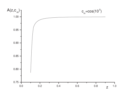
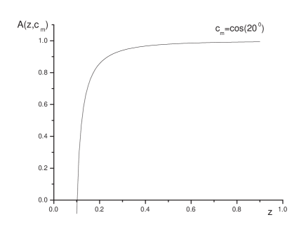
Figure 1: Acceptance factor defined by Eq. (27) for different values of $c_{m}$

Finally, let us note that two representations (21) and (26) for the IES cross section can be obtained also by inserting the QRE form of the leptonic tensor

$$\frac{\alpha}{4\pi^{2}}\frac{d^{3}k}{\omega}L^{\gamma}_{\mu\nu}(p_{1},p_{2},k)\rightarrow\frac{\alpha}{2\pi}P(z,L_{0})\frac{dz}{z}q^{2}\bigl{(}\frac{1}{2}\tilde{g}_{\mu\nu}+\frac{2z^{2}}{q^{2}}\tilde{p}_{1\mu}\tilde{p}_{1\nu}\bigr{)}$$

into Eq. (6).

4 Radiative corrections

If events with $e^{+}e^{-}\pi^{+}\pi^{-}$ final state are rejected, only photonic RC have to be taken into account. These corrections include contributions due to virtual and real soft and hard photon emission. To calculate them we use the QRE approximation from the very beginning.

4.1 Soft and virtual corrections

The soft and virtual corrections are the same for both, unrestricted and restricted pion phase space, and the corresponding contribution can be found by the simple substitution

$$\frac{\alpha}{2\pi}P(z,L_{0})\rightarrow\Bigl{(}\frac{\alpha}{2\pi}\Bigr{)}^{2}C^{S+V}\ ,\ \ C^{S+V}=\rho P(z,L_{0})+D(L_{s},L_{0},z)+N(z)$$ (29)

in the right–hand sides of Eqs. (21) and (26). As a result, we have

$$\frac{d\sigma^{{}^{S+V}}_{F}}{dq^{2}}=\frac{\sigma(q^{2})}{4E^{2}}\Bigl{(}\frac{\alpha}{2\pi}\Bigr{)}^{2}C^{S+V}\ ,\ \ \frac{d\sigma^{{}^{S+V}}_{R}}{dq^{2}}=\frac{d\sigma^{{}^{S+V}}_{F}}{dq^{2}}A(z,c_{m})\ .$$ (30)

All the logarithmically enhanced contributions to $C^{S+V}$ are contained in the first two terms in Eq.(29) and were first found in Ref. [16]. The third term in (29) describes the non–logarithmic contributions [26]. Finally, we obtain

$$\rho=4(L_{s}-1)\ln{\Delta}+3(L_{s}+\ln{z})+\frac{2\pi^{2}}{3}-\frac{9}{2}\ ,L_{s}=\ln{\frac{4E^{2}}{m^{2}}}\ ,$$ (31)

$$D(L_{s},L_{0},z)=\frac{1+z^{2}}{1-z}L_{0}\bigl{[}(L_{0}-2L_{s}-\ln{z})\ln{z}+\frac{\pi^{2}}{3}-2Li_{2}(z)\bigr{]}+\frac{1+2z-z^{2}}{2(1-z)}L_{0}+\frac{4z\ln{z}}{1-z}L_{s}\ ,$$

$$N(z)=-\frac{1}{1-z}-\frac{8z\ln{z}}{1-z}+2z\bigl{[}\ln^{2}(1-z)+\frac{\ln^{2}{z}}{1-z}\bigr{]}+\frac{\pi^{2}}{6}\bigl{(}4z+6-\frac{5}{1-z}\bigr{)}+\bigl{(}4z-6+\frac{5}{1-z}\bigr{)}Li_{2}(z)\ ,$$

where $\Delta E\ (\Delta\ll 1)$ is the maximum energy of a soft photon, and

$$Li_{2}(x)=-\int\limits_{0}^{x}\frac{dy}{y}\ln(1-y)\ .$$

4.2 Two hard photon emission along the electron and positron direction

Concerning the contribution from additional hard photon emission, we divide it into three pieces. The first one is responsible for the radiation of an additional photon with energy $\omega_{2}$ along the positron beam direction (provided that a collinear photon with energy $\omega_{1}$ is emitted along the electron beam direction). To calculate it we introduce the angular auxiliary parameter $\theta_{0}^{\prime}\ll 1$ and use the QRE approximation to describe the radiation of both photons. The calculations are the same for restricted and unrestricted pion phase space and do not affect the acceptance factor (as in the case of virtual and soft corrections). Using the subscript F to indicate the cross-section for the unrestricted phase space, the result reads

$$\frac{d\sigma^{H}_{1F}}{dq^{2}}=\frac{\sigma(q^{2})}{4E^{2}}\int_{y_{0}}^{1-\Delta}\Bigl{(}\frac{\alpha}{2\pi}\Bigr{)}^{2}P(x,L_{0})P(y,L_{0}^{\prime})\frac{dy}{y}\ ,\ L_{0}^{\prime}=\ln{\frac{E^{2}{\theta^{\prime}}_{0}^{2}}{m^{2}}},\ x=1-\frac{\omega_{1}}{E},\ y=1-\frac{\omega_{2}}{E},$$ (32)

where $q^{2}=4E^{2}xy$ is fixed. The maximum value of the photon energy $\omega_{2}$ can be obtained from restriction (3), taking into account that, for the events under consideration, the QRE kinematics $(\cos{\theta_{1}}=1,\ \cos{\theta_{2}}=-1,\ \theta_{1,2}$ are polar angles of photons) gives

$$\Omega=\omega_{1}+\omega_{2},\ \ |{\bf K}|=\omega_{1}-\omega_{2},\ \rightarrow\omega_{2}<\frac{\eta E}{2},\ \ y_{0}=1-\frac{\eta}{2}.$$ (33)

Because of the smallness of the parameter $\eta$, only terms singular at $y=1$ contribute to the integral on the right–hand side of Eq. (32). Moreover, we can substitute $x$ with $z$, neglecting terms of order $\eta$ as compared with unity (because $q^{2}=4E^{2}z=4E^{2}xy)$, and perform an elementary integration over $y$, obtaining

$$\frac{d\sigma^{{}^{H}}_{1F}}{dq^{2}}=\frac{\sigma(q^{2})}{4E^{2}}\Bigl{(}\frac{\alpha}{2\pi}\Bigr{)}^{2}P(z,L_{0})2(L_{0}^{\prime}-1)\ln{\frac{\eta}{2\Delta}}\ ,\ \ \frac{d\sigma^{{}^{H}}_{1R}}{dq^{2}}=\frac{d\sigma^{{}^{H}}_{1F}}{dq^{2}}A(z,c_{m}).$$ (34)

4.3 Two hard photons emitted along the electron directions

The second contribution to the radiative corrections caused by an additional hard photon emission corresponds to the radiation of two hard collinear photons (each of them with energy larger than $\Delta E$) by the electron, provided both are emitted within the narrow cone of opening angle $2\theta_{0}$ along the electron beam direction. This contribution also does not affect the acceptance factor, and the result can be written with the same accuracy as (30) and (32)

$$\frac{d\sigma^{{}^{H}}_{2F}}{dq^{2}}=\frac{\sigma(q^{2})}{4E^{2}}\Bigl{(}\frac{\alpha}{2\pi}\Bigr{)}^{2}C^{{}^{H}}\ ,\ \ \frac{d\sigma^{{}^{H}}_{2R}}{dq^{2}}=\frac{d\sigma^{{}^{H}}_{2F}}{dq^{2}}A(z,c_{m})\ ,$$ (35)

$$C^{{}^{H}}=B_{1}(z,\Delta)L_{0}^{2}+B_{2}(z,\Delta)L_{0}+B_{3}(z,\Delta)\ .$$

Functions $B_{1}(z,\Delta)$ and $B_{2}(z,\Delta)$ were first calculated in Ref. [27]

$$B_{1}(z,\Delta)=\frac{1}{2}P_{2\theta}(z)+\frac{1+z^{2}}{1-z}\bigl{(}\ln z-\frac{3}{2}-2\ln\Delta\bigr{)},$$

$$B_{2}(z,\Delta)=3(1-z)+\frac{(3+z^{2})\ln^{2}z}{2(1-z)}-\frac{2(1+z)^{2}}{1-z}\ln\frac{1-z}{\Delta}\ ,$$ (36)

where $P_{2\theta}(z)$ is the $\theta$–term of the second order electron structure function (see, for example, [28])

$$P_{2\theta}(z)=2\Bigl{[}\frac{1+z^{2}}{1-z}\Bigl{(}2\ln(1-z)-\ln{z}+\frac{3}{2}\Bigr{)}+\frac{1}{2}(1+z)\ln{z}-1+z\Bigr{]}\ .$$

Function $B_{3}(z,\Delta)$ was calculated in Ref. [26] and reads

$$B_{3}(z,\Delta)=\frac{4z}{1-z}\ln\frac{1-z}{\Delta}-\frac{4z}{3(1-z)}-\frac{\pi^{2}}{6}\frac{4z}{3}+\Bigl{(}-\frac{17}{3}+\frac{28}{3(1-z)}-\frac{8}{3(1-z)^{2}}\Bigr{)}\ln{z}+$$ (37)

$$+\frac{3-24z+54z^{2}-48z^{3}+7z^{4}}{6(1-z)^{3}}\ln^{2}z+\bigl{(}1-\frac{7z}{3}\bigr{)}Li_{2}(1-z)+J\ ,$$

$$J=\int\limits_{0}^{1-z}\Bigl{[}\frac{z^{2}+(1-x)^{4}}{x\lambda(1-x)^{2}}\int\limits_{0}^{1}\frac{dt}{t}L(t,x,z)+\frac{z+x}{2(1-x)}L_{1}(x,z)+\frac{x\lambda-3z}{2(1-x)^{2}}L_{2}(x,z)\Bigr{]}dx,$$

where the logarithmic functions $L,\ L_{1}$ and $L_{2}$ are defined as follows

$$L(t,x,z)=\ln{\frac{(1-x)\sqrt{F(t,x,z)}+tx(z-x\lambda)+\lambda(1-x)^{2}}{2\bigl{(}1+\frac{\lambda t}{xz}\bigr{)}\lambda(1-x)^{2}}}\ ,\ \ \lambda=1-x-z,$$

$$L_{1}(x,z)=\ln{\frac{(x+z))\sqrt{F(1,x,z)}+\lambda(z-x\lambda)+x(x+z)^{2}}{2z\lambda}}\ ,$$

$$L_{2}(x,z)=\ln{\frac{(1-x)\sqrt{F(1,x,z)}+x(z-x\lambda)+\lambda(1-x)^{2}}{2\lambda(1-x)^{2}}}\ ,$$

$$F(t,x,z)=\lambda^{2}(1-x)^{2}+2tx\lambda(z-x\lambda)+t^{2}x^{2}(x+z)^{2}\ .$$

The integral over $x$ in the expression for $J$ diverges when $x\rightarrow 0$ and $x\rightarrow 1-z.$ But the structure of the integral is such that these divergences compensate each other, and this can be seen by taking into account that:

i)  integral over $t$ converges,

$$ii)\ \lim\limits_{x\to 0}\ \frac{z^{2}+(1-x)^{4}}{x\lambda(1-x)^{2}}L(t,x,z)=-\frac{1+z^{2}}{x(1-z)}\ln{\frac{t(1-z)}{xz}}\ ,$$

$$iii)\ \lim\limits_{x\to 1-z}\ \frac{z^{2}+(1-x)^{4}}{x\lambda(1-x)^{2}}L(t,x,z)=\frac{1+z^{2}}{\lambda(1-z)}\ln{\frac{t(1-z)}{(1-x-z)z}}\ .$$ (38)

The quantity $J$ can then be computed numerically with appropriate precision. Note also that the integral over $t$ on the right–hand side of Eq. (37) can be computed analytically (see also [29]). i.e.

$$\int\limits_{0}^{1}\frac{dt}{t}L(t,x,z)=\frac{1}{2}L_{2}^{2}(x,z)+Li_{2}\Bigl{(}\frac{2xz}{h}\Bigr{)}+Li_{2}\Bigl{(}-\frac{2x^{2}\lambda}{h}\Bigr{)}+Li_{2}\Bigl{(}-\frac{\lambda}{xz}\Bigr{)}\ ,$$

$$h=\lambda(1-x)^{2}+x(z-x\lambda)+(1-x)\sqrt{F(1,x,z)}\ .$$

4.4 Emission of one hard collinear and one hard wide angle photon with unrestricted pion phase space

The third, least trivial, contribution into the RC caused by two hard photon emission is connected with events when one photon with energy $\omega_{1}$ is collinear and the other (with energy $\omega_{2}$) is radiated at angles between $\pi-\theta_{0}^{\prime}$ and $\theta_{0}.$ For such events, constraints (3) and (4) are somewhat tangled, and one needs to choose convenient variables to disentangle them and to determine the photon phase space. In spite of the obvious fact that these constraints concern only the photons, their respective contribution to the RC affects the acceptance factor given by Eq. (27). The physical reason for such a behaviour is that now (in contrast with previous cases) the 3–momenta of photons and pions do not lie in the same plane even if the QRE kinematics ($k_{1}=(1-x)p_{1})$ is applied.

Nevertheless, the QRE approach for the description of collinear photons allows to simplify the form of the cross section and to disentangle all the kinematical restrictions. In accordance with this approach, the starting point for our calculation of the differential cross section, suitable for the unrestricted pion phase space case, is the following

$$d\sigma^{{}^{H}}_{3F}=\frac{\sigma(q^{2})}{4E^{2}}\frac{\alpha}{2\pi}P(x,L_{0})L^{\gamma}_{\mu\nu}(xp_{1},p_{2},k_{2})\tilde{g}_{\mu\nu}\frac{\alpha}{4\pi^{2}}\frac{dxd^{3}k_{2}}{x\omega_{2}}\ ,$$ (39)

$$\frac{d^{3}k_{2}}{\omega_{2}}=2\pi\omega_{2}d\omega_{2}dc_{2}\ ,\ \ c_{2}=\cos{\theta_{2}}\ ,\ \ x=1-\frac{\omega_{1}}{E}\ ,$$

where $\theta_{2}$ is the polar angle of the non–collinear photon. Since our aim is to derive the differential distribution in the squared pion invariant mass $q^{2}$, it is convenient to use the relation between $q^{2}$ and $c_{2}$ to avoid the integration over $c_{2}$ on the right–hand side of Eq. (39). In addition, it is convenient to introduce the total photon energy $\Omega$ instead of $\omega_{2}$

$$q^{2}=4E(E-\Omega)+2\omega_{1}\omega_{2}(1-c_{2}),\ \ \omega_{2}=\Omega-\omega_{1},\ dc_{2}\rightarrow\frac{dq^{2}}{2\omega_{1}\omega_{2}},\ \ d\omega_{2}=d\Omega\ .$$ (40)

In this case in the lepton tensor $L^{\gamma}_{\mu\nu}$ the electron mass can be neglected. Thus, the differential cross–section has the following form

$$\frac{d\sigma^{H}_{3F}}{dq^{2}}=\frac{\sigma(q^{2})}{4E^{2}}\Bigl{(}\frac{\alpha}{2\pi}\Bigr{)}^{2}\Bigl{\{}P(x,L_{0})\Bigl{[}\frac{2q^{4}}{xu_{1}u_{2}}-2q^{2}\Bigl{(}\frac{1}{xu_{1}}+\frac{1}{u_{2}}\Bigr{)}+\frac{xu_{1}}{u_{2}}+\frac{u_{2}}{xu_{1}}\Bigr{]}\frac{d\omega_{1}d\Omega}{\omega_{1}(E-\omega_{1})}\Bigr{\}}\ ,$$ (41)

$$u_{1}=-2k_{2}p_{1}=-\frac{4E^{2}\Omega_{z}}{\omega_{1}},\ \ u_{2}=-2k_{2}p_{2}=-\frac{4E}{\omega_{1}}[\omega_{1}(\Omega-\omega_{1})-E\Omega_{z}],\ \ \Omega_{z}=\Omega-E(1-z)\ .$$

It is useful to rewrite the expression in curly brackets in a form which is convenient for the integration over $\omega_{1}$ and $\Omega$

$$\Bigl{\{}-L_{0}-\frac{zE^{2}L_{0}}{(E-\omega_{1})^{2}}+\frac{[2z-(1+z)L_{0}]E}{E-\omega_{1}}+\\ \frac{[2(1+z^{2})L_{0}-4z-(1-z)^{2}]E^{2}-(1-z)(\Omega-2\omega_{1})E}{\omega_{1}(\Omega-\omega_{1})-E\Omega_{z}}\Bigr{\}}\frac{d\omega_{1}d\Omega}{E\Omega_{z}}\ ,$$

where we neglect terms which do not contain in the denominator the small quantity $\Omega_{z}$, which is of order $\eta E$, as one can see below from the expressions for $\Omega_{min}$ and $\Omega_{max}.$

Our task now is to define the integration region on the right–hand side of Eq. (41), which is determined by restrictions (3) and (4) for the event selection, as well as by the inequalities

$$-c_{0}^{\prime}<c_{2}<c_{0}\ ,\ \ E\Delta<\omega_{1}<\Omega-E\Delta,\ \ c_{0}^{\prime}=\cos{\theta_{0}^{\prime}},$$ (42)

limiting the possible angles of the non-collinear photon and energies of the collinear one. Restriction (3) defines the maximum value of $\Omega$, whereas restriction (4) defines the minimum value of $\omega_{1}$ at fixed $\Omega$

$$\Omega_{max}=E(1-z)\bigl{(}1+\frac{\eta}{2}\bigr{)}\ ,\ \ \omega_{min}=\frac{2E\Omega_{z}}{\Omega-|{\bf K}|c_{0}}\ ,\ \ |{\bf K}|=\sqrt{\Omega^{2}-4E\Omega_{z}}.$$ (43)

To obtain the minimum value of $\Omega$ we use the first relation in (40) at the minimum possible value of $\omega_{2}=\Delta E$ and $c_{2}=c_{0}$

$$\Omega_{min}\Delta(1-c_{0})=2E[\Omega_{min}-E(1-z)]$$

which leads to

$$\Omega_{min}=E(1-z)\bigl{(}1+\frac{\Delta(1-c_{0})}{2}\bigr{)}\ .$$ (44)

From the condition $c_{2}>-c_{0}^{\prime}$ it follows also that

$$\omega^{-}<\omega_{1}<\omega^{+},\ \ \omega^{\pm}=\frac{\Omega}{2}\bigl{[}1\pm\sqrt{1-\frac{4E\Omega_{z}}{\Omega^{2}}\bigl{(}1+\frac{1-c_{0}^{\prime}}{2}\bigr{)}}\bigr{]}\ .$$ (45)

Finally, inequality $c_{2}<c_{0}$ reads: if the values of $\Omega^{\prime}$s are such that

$$\Omega\leq\Omega_{c}\ ,\ \ \Omega_{c}=E(1-z)\Bigl{(}1+\frac{(1-c_{0})(1-z)}{8}\Bigr{)}$$

then

$$\omega_{1}>\omega_{+}\ \ or\ \ \omega_{1}<\omega_{-},\ \ \omega_{\pm}=\frac{\Omega}{2}\bigl{[}1\pm\sqrt{1-\frac{8E\Omega_{z}}{\Omega^{2}(1-c_{0})}}\bigr{]}.$$ (46)

To derive the integration region we have to combine consistently all constraints (42)–(46) on $\omega_{1}$ and $\Omega$, and such combination leads to

$$\omega_{min}<\omega_{1}<\omega_{-}\ \ and\ \ \omega_{+}<\omega_{1}<\Omega-\Delta E,\ \ \Omega_{min}<\Omega<\Omega_{\Delta}\ ,\ \ \Omega_{\Delta}=E(1-z)(1+\Delta)\ ,$$

$$\omega_{min}<\omega_{1}<\omega_{-}\ \ and\ \ \omega_{+}<\omega_{1}<\omega^{+},\ \Omega_{\Delta}<\Omega<\Omega_{c},$$ (47)

$$\omega_{min}<\omega_{1}<\omega^{+},\ \ \Omega_{c}<\Omega<\Omega_{max}.$$

The integration region defined by the inequalities (47) is shown in Fig. 2.

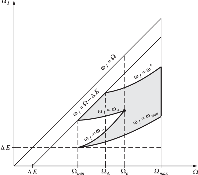
Figure 2: The integration region with respect to $\omega_{1}$ and $\Omega$, as given by inequalities (47)

The integration with respect to $\omega_{1}$ and $\Omega$ on the right–hand side Eq. (40) over the region (47) can be performed analytically, and the list of necessary integrals is

$$\int\frac{d\omega_{1}d\Omega}{E\Omega_{z}}=(1-z)\bigl{(}2-\ln\frac{1+\xi}{\xi}\bigr{)},\ \ \ \xi=\frac{\eta}{(1-c_{0})(1-z)},$$

$$\int\frac{d\omega_{1}d\Omega}{(E-\omega_{1})\Omega_{z}}=-\ln{z}\ln\xi+Li_{2}(1-z)-Li_{2}(-\xi z)+Li_{2}(-\xi)-Li_{2}\bigl{(}-\frac{1-z}{z}\bigr{)},$$

$$\int\frac{Ed\omega_{1}d\Omega}{(E-\omega_{1})^{2}\Omega_{z}}=\frac{1}{z}\bigl{[}-(1+z)\ln{z}-(1-z)\ln\frac{1+\xi z}{\xi}\bigr{]},$$ (48)

$$\int\frac{(\Omega-2\omega_{1})d\omega_{1}d\Omega}{[\omega_{1}(\Omega-\omega_{1})-E\Omega_{z}]\Omega_{z}}=-\frac{\pi^{2}}{6}-\frac{1}{2}\ln^{2}\frac{1-c_{0}}{2}+\ln\frac{\eta}{2\Delta}\ln\frac{(1-c_{0})(1-c_{0}^{\prime})}{4}-2Li_{2}(-\xi),$$

$$\int\frac{Ed\omega_{1}d\Omega}{[\omega_{1}(\Omega-\omega_{1})-E\Omega_{z}]\Omega_{z}}=\frac{1}{1-z}\bigl{[}\frac{\pi^{2}}{2}+\frac{1}{2}\ln^{2}\frac{1-c_{0}}{2}-\ln\frac{\eta}{2\Delta}\ln\frac{(1-c_{0})(1-c_{0}^{\prime})}{4}-\ln^{2}\xi\bigr{]}\ .$$

Using these integrals we can write the corresponding contribution to the IES cross-section from the events presently considered, as follows

$$\frac{d\sigma^{{}^{H}}_{3F}}{dq^{2}}=\frac{\sigma(q^{2})}{4E^{2}}\Bigl{(}\frac{\alpha}{2\pi}\Bigr{)}^{2}\bigl{[}2P(z,L_{0})G_{1}+L_{0}G_{2}+G_{3}\bigr{]}\ ,$$ (49)

$$G_{1}=\frac{\pi^{2}}{2}+\frac{1}{2}\ln^{2}\frac{1-c_{0}}{2}-\ln\frac{\eta}{2\Delta}\ln\frac{(1-c_{0})(1-c_{0}^{\prime})}{4}-\ln^{2}\xi\ ,$$

$$G_{2}=(1-z)\bigl{[}-2+\ln\frac{(1+\xi)(1+\xi z)}{\xi^{2}}\bigr{]}+$$

$$+(1+z)\bigl{[}(1+\ln\xi)\ln{z}+Li_{2}(-\xi z)+Li_{2}\bigl{(}-\frac{1-z}{z}\bigr{)}-Li_{2}(-\xi)-Li_{2}(1-z)\bigr{]},$$

$$G_{3}=-(1-z)\bigl{(}\frac{\pi^{2}}{3}-\ln^{2}\xi\bigr{)}+2Li_{2}(-\xi)+2z\bigl{[}Li_{2}(1-z)-Li_{2}(-\xi z)-Li_{2}\bigl{(}-\frac{1-z}{z}\bigr{)}\bigr{]}.$$

We would like to emphasize that only the part of the IES cross section, defined by Eq. (49), has a non–trivial dependence on the physical parameters $\theta_{0}$ and $\eta$, which determine the main requirements for the event selection.

4.5 Emission of one hard collinear and one hard wide angle photon with restricted pion phase space

Consider now the situation with restricted pion phase space. Unfortunately, the calculations in this case are not so simple and cannot be performed analytically. Nevertheless, the dependence on the unphysical auxiliary parameters $\Delta$ and $\theta_{0}^{\prime}$, which have to vanish in final result for total RC, can be extracted.

Our starting point is the following representation for the differential cross section corresponding to the QRE approximation (by analogy with (39))

$$d\sigma^{{}^{H}}_{3R}=\frac{12\sigma(q^{2})}{4E^{2}q^{2}\zeta}\frac{\alpha^{2}}{8\pi^{2}}P(x,L_{0})\frac{dx}{x}L^{\gamma}_{\mu\nu}(xp_{1},p_{2},k_{2})(-\tilde{p}_{-\mu}\tilde{p}_{-\nu})\frac{d^{3}k_{2}}{\omega_{2}}\frac{d\varphi_{-}}{2\pi}Hdc_{-}\ ,$$ (50)

$$H=\frac{|{\bf p}_{-}|^{2}}{(2E-\Omega)|{\bf p}_{-}|+E_{-}[\omega_{1}c_{-}+(\Omega-\omega_{1})c_{2_{-}}]}\ ,\ \ c_{2_{-}}=c_{2}c_{-}+s_{2}s_{-}\cos{(\varphi_{2}-\varphi_{-})}\ ,\ s_{2}=\sin{\theta_{2}},$$

where $\varphi_{2}$ is the azimuthal angle of the non–collinear photon.

The experience of previous calculations in the case of unrestricted pion phase space suggests that, in order to express the pion energy via angles and photon energies, we can use $\Omega=E(1-z),$ neglecting only small terms of order $\eta$ as compared with unity. Therefore, we have

$$E_{-}=\frac{2Ez(\bar{A}-\bar{K}\bar{B})}{\bar{A}^{2}-\bar{B}^{2}}\ ,\ \ \bar{K}=\sqrt{1-\frac{\delta^{2}}{z^{2}}(\bar{A}^{2}-\bar{B}^{2})}\ ,\ \ \bar{A}=1+z\ ,\ \ \bar{B}=(1-x)c_{-}+(x-z)c_{2-}\ ,$$ (51)

and with the same accuracy

$$H=\frac{2z(\bar{A}\bar{K}-\bar{B})^{2}}{\bar{K}(\bar{A}^{2}-\bar{B}^{2})^{2}}\ ,\ \ E_{+}=E(1+z)-E_{-}\ .$$ (52)

In the limiting case when the energy of the non–collinear photon approaches zero $(x=z),$ $H$ becomes twice the corresponding value entering, under integral sign, into the expression for the acceptance factor (27)

$$\lim\limits_{x\to z}H=H_{s}=\frac{2z[(1+z)K-(1-z)c_{-}]^{2}}{K[(1+z)^{2}-(1-z)^{2}c_{-}^{2}]^{2}}\ .$$ (53)

The upper limit of the $c_{-}$ variation has to be determined from the 3–momentum conservation, provided that $\theta_{+}=\pi-\theta_{m},$ that is

$$-|{\bf p}_{+}|c_{m}+|{\bf p}_{-}|c_{-}+E[1-x+(x-z)c_{2}]=0\ ,$$ (54)

where one has to use expressions for $E_{-}$ and $E_{+}$ to find $|{\bf p}_{+}|$ and $|{\bf p}_{-}|$ as given by (51) and (52).

Contracting the indices on the right–hand side of Eq. (50) and using relations (40) we arrive at the distribution over the squared di–pion invariant mass

$$\frac{d\sigma^{{}^{H}}_{3R}}{dq^{2}}=\frac{12\sigma(q^{2})}{4E^{2}\zeta}\Bigl{(}\frac{\alpha}{2\pi}\Bigr{)}^{2}P(x,L_{0})\frac{d\omega_{1}d\Omega}{(E-\omega_{1})\omega_{1}}\frac{TH}{2}\frac{d(\varphi_{2}-\varphi_{-})}{2\pi}dc_{-}\ ,\ \ x=1-\frac{\omega_{1}}{E}\ ,$$ (55)

$$T=-\frac{\delta^{2}}{z}\Bigl{[}\frac{(q^{2}-xu_{1})^{2}+(q^{2}-u_{2})^{2}}{xu_{1}u_{2}}\Bigr{]}+\frac{\chi_{1}(q^{2}-u_{2})}{u_{1}u_{2}}+\frac{\chi_{2}(q^{2}-xu_{1})}{xu_{1}u_{2}}-\frac{x^{2}\chi_{1}^{2}+\chi_{2}^{2}}{xu_{1}u_{2}}\ .$$

To advance further, one must integrate first over $c_{-}$ because the upper limit $c_{max}$ depends on $c_{2}$ (as it follows from (54)), and in its turn $c_{2}$ is a function of $q^{2}$ and of the variables $\omega_{1}$ and $\Omega.$ In the general case we cannot integrate analytically, even to write the analytical expression for $c_{max}$ is a problem. But it is necessary to prepare the expressions which can then be integrated numerically. Therefore, the dependence on the unphysical parameters $\Delta$ and $\theta_{0}^{\prime}$ has to be extracted.

For this goal, note first that $\Delta E$ is the minimum possible energy for the non–collinear photon. Therefore, in order to extract the $\Delta$–dependence it is sufficient to investigate the limit $\omega_{2}\rightarrow 0.$ In this limiting case $x=z$, and we can use Eq. (53) for the term $H$. Moreover, the 3–momentum conservation (54) becomes the same as in the Born approximation, and its solution $c_{max}(\omega_{2}\rightarrow 0)$ coincides with the expression given in (28).

Next, we select terms in the expression for $T$ that are singular in this soft limit, because only such terms lead to the $\Delta$–dependence via $\ln{\Delta}.$ From the list of integrals (48) and the expression for $u_{1},\ u_{2}$ (see (41)), it is easy to understand that only the terms containing the product $u_{1}u_{2}$ in the denominator can induce such a dependence. Taking into account also that, in this limiting case, $\chi_{2}=q^{2}-z\chi_{1},$ the necessary terms can be written in the following form

$$T_{s}=\frac{2U16E^{2}}{u_{1}u_{2}}=\frac{2E^{3}z(1-z)^{2}U}{\Omega_{z}[\omega_{1}(\Omega-\omega_{1})-E\Omega_{z}]}$$ (56)

(for the definition of $U$ see Eq. (27)). To extract the $\ln{\Delta}$–dependence we apply the standard subtraction procedure and rewrite the cross section (55) as the sum of its hard and soft parts

$$\frac{d\sigma^{{}^{H}}_{3R}}{dq^{2}}=\frac{d\sigma^{{}^{H_{h}}}_{3R}}{dq^{2}}+\frac{d\sigma^{{}^{H_{s}}}_{3R}}{dq^{2}}\ ,$$ (57)

where

$$\frac{d\sigma^{{}^{H_{s}}}_{3R}}{dq^{2}}=\frac{12\sigma(q^{2})}{4E^{2}\zeta}\Bigl{(}\frac{\alpha}{2\pi}\Bigr{)}^{2}P(z,L_{0})\frac{d\omega_{1}d\Omega T_{s}H_{s}}{2E^{2}z(1-z)}dc_{-}\ ,$$ (58)

and the upper limit of $c_{-}$ variation in Eq. (58) is defined by Eq. (28). The hard part of the cross section on the right–hand side of Eq. (57) is not singular at $\omega_{2}\rightarrow 0$, whereas the integration of the soft part over the region (47) induces all $\Delta$–dependence. Using the corresponding formula in the list of integrals (48) we present the soft part of cross section (55) in the form

$$\frac{d\sigma^{{}^{H_{s}}}_{3R}}{dq^{2}}=\frac{\sigma(q^{2})}{4E^{2}}\Bigl{(}\frac{\alpha}{2\pi}\Bigr{)}^{2}P(z,L_{0})G_{1}A(z,c_{m})\ ,$$ (59)

where $G_{1}$ is defined in Eq. (49).

It is worth noting that this soft part absorbs also all the dependence on the angular auxiliary parameter $\theta_{0}^{\prime}.$ That is the reason why the hard part of the cross section depends on the physical parameters only and can be computed numerically. The soft part (58) of the cross section has to be added to the other contributions into the RC to eliminate the dependence on the unphysical parameters in the total RC.

5 Total radiative correction

The total contribution from radiative corrections to the Born cross section in the case of unrestricted pion phase space is represented by the sum

$$\frac{d\sigma^{{}^{RC}}_{F}}{dq^{2}}=\frac{d\sigma^{{}^{S+V}}_{F}}{dq^{2}}+\frac{d\sigma^{{}^{H}}_{1F}}{dq^{2}}+\frac{d\sigma^{{}^{H}}_{2F}}{dq^{2}}+\frac{d\sigma^{{}^{H}}_{3F}}{dq^{2}}\ ,$$ (60)

whereas for the case of restricted phase space we have

$$\frac{d\sigma^{{}^{RC}}_{R}}{dq^{2}}=\frac{d\sigma^{{}^{S+V}}_{R}}{dq^{2}}+\frac{d\sigma^{{}^{H}}_{1R}}{dq^{2}}+\frac{d\sigma^{{}^{H}}_{2R}}{dq^{2}}+\frac{d\sigma^{{}^{H_{s}}}_{3R}}{dq^{2}}+\frac{d\sigma^{{}^{H_{h}}}_{3R}}{dq^{2}}\ .$$ (61)

The two auxiliary parameters, the infrared cut–off $\Delta$ and the collinearity angle $\theta_{0}^{\prime},$ enter into the individual terms on the right–hand sides of Eq. (60) and (61) in the same combination

$$2P(z,L_{0})\ln\Delta\bigl{[}2(L_{s}-1)-(L_{0}^{\prime}-1)-(L_{0}-1)+\ln\frac{\theta_{0}^{2}{\theta^{\prime}}_{0}^{2}}{16}\bigr{]}\ ,$$ (62)

(here and below we use the expansion of $c_{0}$ and $c_{0}^{\prime}$). According to the definition of the large logarithms $L_{0},\ L_{s}$ and $L_{0}^{\prime}$ (see Eqs. (17), (31) and (32)), the expression in square brackets in Eq. (62) equals to zero, and, therefore, the total RC depends only on physical parameters and can be written, in the case of unrestricted phase space, as

$$\frac{d\sigma^{{}^{RC}}_{F}}{dq^{2}}=\frac{\sigma(q^{2})}{4E^{2}}\frac{\alpha}{2\pi}P(z,L_{0})\delta^{{}^{RC}}_{F},\ \ \delta^{{}^{RC}}_{F}=\frac{\alpha}{2\pi}\frac{F_{0}+L_{0}F_{1}+F_{2}}{P(z,L_{0})}\ ,$$ (63)

$$F_{0}=\frac{1}{2}L_{0}^{2}P_{2\theta}(z)+P(z,L_{0})\bigl{[}L_{s}\bigl{(}\frac{3}{2}+2\ln\frac{\eta}{2}\bigr{)}+\ln\frac{4}{\theta_{0}^{2}}\bigl{(}\frac{3}{2}+2\ln\frac{\eta}{z\theta_{0}}\bigr{)}-2\ln^{2}\xi-2\ln\frac{\eta}{2}+3\ln{z}+\frac{5\pi^{2}}{3}-\frac{9}{2}\bigr{]}\ ,$$

$$F_{1}=\frac{3-8z+z^{2}}{2(1-z)}-\frac{2(1+z)^{2}}{1-z}\ln(1-z)+\bigl{[}\frac{4z}{1-z}+(1+z)(1+\ln\xi)\bigr{]}\ln{z}+\frac{1}{2}(1+z)\ln^{2}z+\frac{1+z^{2}}{1-z}\bigl{(}\frac{\pi^{2}}{3}-$$

$$-2Li_{2}(z)\bigr{)}+(1-z)\ln\frac{(1+\xi)(1+\xi z)}{\xi^{2}}+(1+z)\bigl{[}Li_{2}(-\xi z)+Li_{2}\bigl{(}-\frac{1-z}{z}\bigr{)}-Li_{2}(-\xi)-Li_{2}(1-z)\bigr{]},$$

$$F_{2}=(1-z)\ln^{2}\xi-\frac{3+4z}{3(1-z)}+\frac{4z}{1-z}\ln(1-z)+\bigl{[}-2z\ln\xi+\frac{3-18z+7z^{2}}{3(1-z)^{2}}\bigr{]}\ln{z}+2z\ln^{2}(1-z)+$$

$$+\frac{3-12z+30z^{2}-36z^{3}+7z^{4}}{6(1-z)^{3}}\ln^{2}z+\frac{\pi^{2}}{6}\bigl{(}4+\frac{14z}{3}-\frac{5}{1-z}\bigr{)}+Li_{2}(z)\bigl{(}4z-6+\frac{5}{1-z}\bigr{)}+$$

$$+\bigl{(}1-\frac{z}{3}\bigr{)}Li_{2}(1-z)+2Li_{2}(-\xi)-2z\bigl{[}Li_{2}(-\xi z)+Li_{2}\bigl{(}-\frac{1-z}{z}\bigr{)}\bigr{]}+J\ .$$

As mentioned in the Introduction, the IES Born cross section and its RC factorize into the low energy pion pair production cross–section, $\sigma(q^{2}),$ and a term of a pure electrodynamical origin. This latter term depends on the measured pion invariant mass $q^{2}$ and on the physical parameters $\eta$ and $\theta_{0}$ which define the rules for the IES.

Figure 3: The full first order radiative correction to the Born cross section (21) for the case of unrestricted pion phase space, as defined by Eq. (63)

The $z$–dependence of the total radiative correction to the Born cross section (21),$\delta^{{}^{RC}}_{F}$, is shown in Fig. 3. Note that the contribution of the non–logarithmic terms to $\delta^{{}^{RC}}_{F}$ equals parametrically to $\alpha/(2\pi L_{0})$, which is of order $10^{-4}$, as the relative contribution of terms proportional to ${\bf P}_{\Phi}^{2}/4E^{2}$ and $\theta_{0}^{2}/6$ in the Born cross section (see Eq. (20)). That is why the exact calculation of the Born IES cross-section should be complemented with the radiative corrections calculated with the inclusion of non–logarithmic contributions.

Similarly to (63), we can write the complete radiatively corrected cross-section for the case of restricted pion phase space in the form

$$\frac{d\sigma^{{}^{RC}}_{R}}{dq^{2}}=\frac{\sigma(q^{2})}{4E^{2}}\frac{\alpha}{2\pi}P(z,L_{0})A(z,c_{m})\delta^{{}^{RC}}_{R}+\frac{d\sigma^{{}^{H_{h}}}_{3R}}{dq^{2}}\ ,$$ (64)

where

$$\delta^{{}^{RC}}_{R}=\frac{\alpha}{2\pi}\frac{F_{0}+L_{0}F_{1R}+F_{2R}}{P(z,L_{0})}\ \ ,F_{1R}=F_{1}-G_{2}\ ,\ \ F_{2R}=F_{2}-G_{3}\ .$$ (65)

Because the factor $\sigma(q^{2})/4E^{2}$ enters into the last term at the right–hand side of Eq. (64) also, the total RC in this case has a factorized form as well.

There exists one more contribution caused by two hard photon emission when neither photon is emitted within the narrow cone along the the electron beam direction but, nevertheless, the collinear condition (4) is satisfied. This contribution cannot be calculated by the QER approach and has to be evaluated by other methods. In particular, the double bremsstrahlung lepton current tensor can be taken in limit $m\rightarrow 0.$ To our understanding, due to the strong constraint (3) on the event selection, the corresponding contribution is small enough and does not affect the IES cross section on the one per cent level. Nevertheless, the theoretical evaluation of this contribution should be done and we hope to compute it elsewhere.

6 Pair production contribution into the IES cross section

The above considerations for the photonic radiative corrections to the IES cross section are appropriate if $e^{+}e^{-}\pi^{+}\pi^{-}$ final states are excluded from the analysis. If not, there is an additional contribution caused by hard initial–state radiation with $e^{+}e^{-}$ pair production [16]. The main part of this contribution arises due to collinear kinematics. In the framework of the NLO approximation, where only logarithmically enhanced terms are kept, the corresponding cross section can be written as

$$\frac{d\sigma^{e^{+}e^{-}(c)}_{F}}{dq^{2}}=\frac{\sigma(q^{2})}{4E^{2}}\Bigl{(}\frac{\alpha}{2\pi}\Bigr{)}^{2}\bigl{[}P_{1}(z)L_{0}^{2}+P_{2}(z)L_{0}\bigr{]}\ ,\ \ \frac{d\sigma^{e^{+}e^{-}(c)}_{R}}{dq^{2}}=\frac{d\sigma^{e^{+}e^{-}(c)}_{F}}{dq^{2}}A(z,c_{m})\ ,$$ (66)

where the functions $P_{1}(z)$ and $P_{2}(z)$ can be extracted from the corresponding results for small–angle Bhabha scattering cross–section, given in Ref. [30]. We present them here for completeness, i.e.

$$P_{1}(z)=\frac{1+z^{2}}{3(1-z)}+\frac{(1-z)(4+7z+4z^{2})}{6z}+(1+z)\ln{z}\ ,$$

$$P_{2}(z)=-\frac{107}{9}+\frac{136}{9}z-\frac{2}{3}z^{2}-\frac{4}{3z}-\frac{20}{9(1-z)}+\frac{2}{3}\Bigl{(}-4z^{2}+5z+1+\frac{4}{z(1-z)}\Bigr{)}\ln(1-z)$$

$$+\frac{1}{3}\Bigl{(}8z^{2}+5z-7-\frac{13}{1-z}\Bigr{)}\ln{z}-\frac{2}{1-z}\ln^{2}z+4(1+z)\ln{z}\ln(1-z)-\frac{2(3z^{2}-1)}{1-z}Li_{2}(1-z)\ .$$

Within the NLO accuracy, one has to compute also the contribution caused by the semicollinear kinematics of the $e^{+}e^{-}$ pair production, when the final state electron belongs to the narrow cone along the electron beam direction while the positron does not. The corresponding part of the leptonic tensor was derived in [31], and has the form

$$L_{\mu\nu}^{e+e-}=-\frac{\alpha^{2}}{4\pi^{3}}\frac{d^{3}k_{+}d\,x(1+x^{2})}{\varepsilon_{+}(1-x)^{2}sv_{1}}L_{0}\Bigl{\{}\Bigl{[}\frac{s^{2}+v_{1}^{2}}{2}+\frac{q^{2}v_{2}}{(1-x)^{2}}\Bigr{]}\tilde{g}_{\mu\nu}+\frac{2q^{2}}{(1-x)^{2}}(\tilde{p}_{2\mu}\tilde{p}_{2\nu}+\tilde{k}_{+\mu}\tilde{k}_{+\nu})\Bigr{\}}\ ,$$

where $k_{+}\ (\varepsilon_{+})$ is the 4 – momentum (energy) of the non–collinear positron, $x$ is the energy fraction of the collinear electron and $v_{1,2}=-2p_{1,2}k_{+}.$

For unrestricted pion phase space, the differential cross section can be written as follows

$$\frac{d\sigma^{e+e-(s)}_{F}}{dq^{2}}=\frac{\sigma(q^{2})}{4E^{2}}\Bigl{(}\frac{\alpha}{2\pi}\Bigr{)}^{2}L_{0}\frac{d\Omega dx}{\Omega_{z}}\frac{(1+x^{2})[(1-x-z)^{2}+z^{2}]}{(1-x)^{4}}\ ,$$ (67)

Neglecting terms of order $m/E,$ we can integrate over the region shown in Fig. 2 with the substitution $\omega/E\rightarrow x.$ In addition to the list of integrals (48), it is necessary to compute the following ones

$$\int\frac{dx\,d\Omega}{(1-x)^{3}\Omega_{z}}=\frac{(1-z)^{2}\xi}{2z(1+z\xi)}+\frac{1-z^{2}}{2z^{2}}\Bigl{(}1+\ln\frac{1+z\xi}{\xi}\Bigr{)}-\frac{1+z^{2}}{2z^{2}}\ln{z}\ ,$$

$$\int\frac{dx\,d\Omega}{(1-x)^{4}\Omega_{z}}=\frac{(1-z)(3+z)}{3z^{3}}+\frac{(1-z)^{3}}{6z^{3}(1+z\xi)^{2}}-\frac{(1-z)^{2}(2+z)}{3z^{3}(1+z\xi)}-$$ (68)

$$-\frac{1+z^{3}}{3z^{3}}\ln{z}-\frac{1-z^{3}}{3z^{3}}\ln\frac{1+z\xi}{\xi}\ .$$

Figure 4: The radiative correction to the IES Born cross section caused by $e^{+}e^{-}$–pair production

Using integrals (48), (68) and the definition (67), the contribution of the semicollinear kinematics of pair production into the IES cross section can be written in the form

$$\frac{d\sigma^{e+e-(s)}_{F}}{dq^{2}}=\frac{\sigma(q^{2})}{4E^{2}}\Bigl{(}\frac{\alpha}{2\pi}\Bigr{)}^{2}L_{0}S(z,\xi)\ ,$$ (69)

$$S(z,\xi))=(1-z)\Bigl{\{}\ln\frac{\xi}{1+\xi}-\frac{2}{3}\Bigl{[}1+\frac{(1-z)^{2}\xi}{(1+z\xi)^{2}}+\frac{2(1+z+z^{2})}{z}\ln\frac{1+z\xi}{\xi}\Bigr{]}\Bigr{\}}+$$

$$2(1+z)\Bigl{[}\Bigl{(}\ln{\xi}-\frac{2}{3z}(1-z+z^{2})\Bigr{)}\ln{z}+Li_{2}(-z\xi)+Li_{2}\bigl{(}-\frac{1-z}{z}\bigr{)}-Li_{2}(1-z)-Li_{2}(-\xi)\Bigr{]}\ .$$

The contribution of $e^{+}e^{-}$ pair production into the IES cross section for the case of unrestricted pion phase space now reads

$$\frac{d\sigma^{{}^{e+e-}}_{F}}{dq^{2}}=\frac{\sigma(q^{2})}{4E^{2}}\frac{\alpha}{2\pi}P(z,L_{0})\delta^{{}^{e+e-}}_{F},\ \ \delta^{{}^{e+e-}}_{F}=\frac{\alpha}{2\pi}\frac{P_{1}(z)L_{0}^{2}+(P_{2}(z)+S(z,\xi))L_{0}}{P(z,L_{0})}\ .$$ (70)

with the function $\delta^{{}^{e+e-}}_{F}$ shown in Figure 4. In the case of restricted pion phase space, the differential distribution over the pion squared invariant mass can be written, in analogy with Eq. (55), in the following form

$$\frac{d\sigma^{e^{+}e^{-}(s)}_{R}}{dq^{2}}=\frac{12\sigma(q^{2})}{4E^{2}\zeta}\Bigl{(}\frac{\alpha}{2\pi}\Bigr{)}^{2}L_{0}\frac{(1+x^{2})d\,xd\Omega}{(1-x)^{4}\Omega_{z}}\frac{T_{p}H_{p}}{2}dc_{-}\frac{d(\tilde{\varphi}_{+}-\varphi_{-})}{2\pi}\ ,$$ (71)

where the integration region in $x$ and $\Omega$ is the same as in (67). Here, we use the following notation

$$T_{p}=-\frac{\delta^{2}}{z^{2}}[z^{2}+(1-x-z)^{2}]+x\tilde{\chi}_{2}+(1-x-z)\tilde{\chi}_{+}+\tilde{\chi}_{2}^{2}+\tilde{\chi}_{+}^{2}\ ,\ \ \tilde{\chi_{2}}=\frac{\chi_{2}}{4E^{2}}\ ,\ \ \tilde{\chi}_{+}=\frac{2k_{+}p_{-}}{4E^{2}}\ ,$$

$$H_{p}=\frac{2z(\widetilde{A}\widetilde{K}-\widetilde{B})^{2}}{\widetilde{K}(\widetilde{A}^{2}-\widetilde{B}^{2})^{2}}\ ,\ \ \widetilde{A}=A,\ \ \widetilde{B}=xc_{-}=(1-x-z)c_{+-}\ ,$$

$$c_{+-}=\tilde{c}_{+}c_{-}+\tilde{s}_{+}s_{-}\cos{(\tilde{\varphi}_{+}-\varphi_{-})}\ ,\ \ \tilde{c}_{+}=\cos{\tilde{\theta}_{+}}\ ,\ \ \tilde{s}_{+}=\sin{\tilde{\theta}_{+}}\ ,$$

and $\tilde{\theta}_{+},\ \tilde{\varphi}_{+}$ are polar and azimuthal angles of the final non-colinear positron.

For the further integration on the right–hand side of Eq. (71) with respect to the angular pion phase space, one must determine the upper limit of $c_{-}$ variation. It depends on $q^{2},\ x,\ \Omega$ and $\cos{(\tilde{\varphi}_{+}-\varphi_{-})}$ and can be obtained as a solution of the equation

$$-|{\bf p}_{+}|c_{m}+|{\bf p}_{-}|c_{-}+E(x+(1-x-z)\tilde{c_{+}})=0\ ,$$ (72)

taking into account that

$$E_{-}=\frac{2Ez(\widetilde{A}-\widetilde{K}\widetilde{B})}{\widetilde{A}^{2}-\widetilde{B}^{2}}\ ,\ \ E_{+}=E(1+z)-E_{-}\ .$$

The total contribution of $e^{+}e^{-}$–pair production into IES cross section for the case of restricted pion phase space

$$\frac{d\sigma^{e+e-}_{R}}{dq^{2}}=\frac{d\sigma^{e+e-(c)}_{R}}{dq^{2}}+\frac{d\sigma^{e+e-(s)}_{R}}{dq^{2}}$$ (73)

has no singularity and can be calculated numerically.

We have considered in the above the contribution of kinematic regions where at least one collinear photon or an electron–positron pair is radiated by the initial electron. DA$\Phi$NE conditions allow to select and detect also the same events when the collinear particles are emitted by the initial positron. Therefore, all the cross sections derived above have to be doubled.

7 Conclusion

The success of precision studies of the hadronic cross section in electron–positron annihilation through the measurement of radiative events [18, 21, 22] relies on the matching level of reliability of the theoretical expectations. The principal problem is the analysis of radiative corrections corresponding to realistic conditions for event selection.

In previous work [20] we discussed briefly an inclusive approach to the measurement of the hadronic cross section at DA$\Phi$NE in the region below $1\ GeV$ by the radiative return method, for the case in which the radiated photon remains untagged. This approach requires an exact knowledge of the final hadronic state and a precise determination of its invariant mass. Some additional constraints have to be imposed to make the detection of the ISR photon redundant and to avoid any uncertanties in the interpretation of the selected events. These additional constraints imply also the precise measurement of the pion 3–momenta. The KLOE detector at DA$\Phi$NE offers a very promising possibility to realize such an inclusive approach to the scanning of the hadronic cross section by the ISR events.

In this paper we compute the corresponding ISR Born cross section and the radiative corrections to it in the framework of the QRE approximation. It is shown that this approximation is quite appropriate, even at the Born level, and provides high accuracy for the IES cross section. The cases of unrestricted and restricted pion phase space are considered. In the first case the photonic contribution to the RC is calculated analytically with the NNLO accuracy and the contribution caused by $e^{+}e^{-}$–pair production within the NLO. The photonic RC is large and negative in a wide range of pion invariant masses. The physical reason for such behaviour of the photonic RC is very transparent: the phase space of additional real photon is restricted considerably by the constraints (3) and (4), and the respective positive contribution cannot compensate the negative contribution due to the virtual correction. The large absolute value of the first order photonic correction indicates unambiguously that the second order RC has to be evaluated. Moreover, the increase of the soft part of the RC (when $z$ grows and approaches unity) requires summation of the leading RC to all orders.

If the entire phase space for photons and $e^{+}e^{-}$–pairs is allowed, this problem is solved by the ordinary Drell–Yan–like representation in electrodynamics [32, 33] with the exponential form of the electron structure functions [28, 34]. For the tagged collinear photon events without any constraints on the phase space of additional particles, the corresponding representation was derived in Ref. [16], but the case considered here requires special investigation because of two non–trivial constraints (3) and (4) on the event selection. We hope to consider this problem elsewhere.

The RC caused by $e^{+}e^{-}$–pair production is positive and small, as compared with the absolute value of the photonic correction. Only in the region near threshold (small $z$), where the cross section is very small, it approaches approximately the same value. So, we conclude that the RC due to pair production described by Eq. (70) is adequate, and it must be taken into account to guarantee the one per cent accuracy.

In the case of restricted pion phase space, we derived the analytical form of the acceptance factor for the Born cross section and the part of RC which includes contributions due to vitrual and real collinear photons and $e^{+}e^{-}$ pair. Even the choice of the detected pion angles between $20^{o}$ and $160^{o}$ gives a value of the acceptance factor very close to unity, providing good statistics at all values of the hadron invariant mass. Concerning the contribution into the IES cross section caused by the semicollinear kinematics for the double photon emission and pair production, the respective acceptance factor cannot be calculated analytically. In this case formulae suitable for numerical calculation are given.

One of the advantages of the IES approach discussed in this paper is a considerable decrease of the FSR background. The corresponding contribution into the IES cross section is suppressed by factors of order $\theta_{0}^{2}$ due to the collinear restriction (4) on event selection, therefore we can ignore any RC to the FSR events and evaluate this background only at the Born level. The same is valid for the contribution caused by the ISR–FSR interference. Note that, for the tagged photon setup, the corresponding background is quite large and, in order to obtain the one per cent accuracy [19], one needs evaluate the radiative corrections to it. If events with $e^{+}e^{-}\pi^{+}\pi^{-}$ final state cannot be excluded by the experimental selection, the background due to the double photon mechanism of $\pi^{+}\pi^{-}$–pair production has to be evaluated as well. To our understanding, this background contains the same suppression factor $\theta_{0}^{2}$. In addition, restriction (3) selects very specific kinematics and does not allow to reach the region where the virtualities of both intermediate photons are small, and the corresponding cross section is the largest. In fact, due to this restriction, at least, one of the photons becomes far off-shell (with virtuality of the order $-q^{2}$). Thus, we expect that double photon mechanism contributes at the level of the RC to the FRS and cannot affect the IES cross section at the one per cent level.

Authors thank G. Venanzoni for fruitful discussion. V.A.K. is grateful to The Leverhulme Trust for a Fellowship. N.P.M. thanks INFN and Parma University for the hospitality. G. P., acknowledges support from EEC Contract TMR98-0169.

References

- [1] R.M. Carey et al., (g-2) Collaboration, Phys. Rev. Lett. 82, 1632 (1999); H.M. Brown et al., (g-2) Collaboration, Phys. Rev. D 62, 0901101 (2000); Phys. Rev. Lett. 86, 2227 (2001); B. Lee Roberts et al., (g-2) Collaboration, hep-ex/0111046.
- [2] For recent reviews see, for example, A.H. Hőcker, hep–ph/0111243; J.F. de Trocóniz, F.J. Yndurain, hep–ph/0111258.
- [3] V.W. Hugles and T. Kinoshita, Rev. Mod. Phys. 71, 133 (1999).
- [4] A.Czarnecki, W.J. Marciano, hep–ph/0102122; W.J. Marciano, B.L. Roberts, hep–ph/0105056; K. Melnikov, SLUC–PUB–8844, hep–ph/0105267; F.J. Yndurain, hep–ph/0102312; F.Jegerlehner, hep–ph/0001386, hep–ph/0104304; A. Widom and Y. Srivastava, hep–ph/011135v1.
- [5] M.Knecht and A.Nyffeler,hep-ph/0111058; M. Knecht, A Nyffeler, M. Perrotet and E. de Rafael, hep–ph/0111059.
- [6] M.Hayakawa and T.Kinoshita, hep-ph/0112102.
- [7] J. Bijnens, E.Pallante and J.Prades, hep-ph/0112255.
- [8] M.Davier and H. Hőcker, Phys. Lett. B 419, 419 (1998), B 435, 427 (1998).
- [9] S. Eidelman, F. Jegerlehner, Z. Phys. C 67, 585 (1995); F. Jegerlehner, Preprint DESY 99–07, hep–ph/9901386.
- [10] N. Cabibbo, R. Gatto, Phys. Rev 124, 1577 (1961).
- [11] R.R. Akhmetshin et al., hep–ex/9904027; Nucl. Phys. A 675, 424 (2000); Phys. Lett. B 475, 190 (2000).
- [12] D. Kong, hep-ph/9903521; J.Z.Bai et al., BES Collaboration, Phys. Rev. Lett. 84, 594 (2000); hep–ex/0102003.
- [13] F. Jegerlehner, LC-TH-2001-035, DESY-01-029, in: 2nd ECFA/DESY Study 1998-2001, 1851, (hep-ph/0105283).
- [14] F. Jegerlehner, hep–ph/0104304.
- [15] V.N. Baier, V.A. Khoze, Sov. Phys. JETP, 21, 629 (1965); Sov. Phys. JETP, 21, 1145 (1965).
- [16] A.B. Arbuzov, E.A. Kuraev, N.P. Merenkov, L. Trentadue, JHEP 12 (1998) 009.
- [17] S. Binner, J.H. Kűhn and K. Melnikov, Phys. Lett. B 459, 279 (1999); M. Konchatnij, N.P. Merenkov, JETP. Lett. 69, 811 (1999); S. Spagnolo, Eur. Phys. J. C 6, 637 (1999); J.Kűhn , Nucl. Phys. Proc. Suppl. 98, 289-296 (2001).
- [18] G. Cataldi, A. Denig, W. Kluge, G. Venanzoni, KLOE MEMO 195, August 13, 1999.
- [19] A. Hoefer, J. Gluza, F. Jegerlehner, hep-ph/0107154.
- [20] V.A. Khoze, M.I. Konchatnij, N.P. Merenkov, G. Pancheri, L. Trentadue, O.N. Shekhovzova, Eur. Phys. J. C 18, 481 (2001).
- [21] G. Cataldi et al., Physics and Detectors at DANE, 569 (1999).
- [22] A.Aloisio et al, KLOE Collaboration, hep-ex/0107023; A. Denig (on behalf of KLOE Collaboration), hep-ex/0106100.
- [23] G.Rodrigo et al, hep-ph/0106132; G. Rodrigo, hep–ph/0111151.
- [24] V.N. Baier, V.S. Fadin, V.A. Khoze, Nucl. Phys. B 65, 381 (1973).
- [25] E.A. Kuraev, N.P. Merenkov, V.S. Fadin, Sov. J. Nucl. Phys. 45, 486 (1987).
- [26] G.I. Gakh, M.I. Konchatnij, N.P. Merenkov, O.N. Shekhovzova, Ukr. Fiz. Zh. 46, 652 (2001).
- [27] N.P. Merenkov, Sov. J. Nucl. Phys. 48, 1073 (1988).
- [28] S. Jadach, M. Skrzypek, B.F.L. Ward, Phys. Rev. D 47, 3733 (1993); S. Catani, L. Trentadue, JETP Lett. 51, 83 (1990).
- [29] H. Anlauf, hep–ph/0110120.
- [30] A.B. Arbuzov, E.A. Kuraev, N.P. Merenkov, L. Trentadue, JETP 81, 638 (1995).
- [31] M.I. Konchatnij, N.P. Merenkov, O.N. Shekhovzova, JETP 91, 1 (2000).
- [32] E.A. Kuraev, V.S. Fadin, Sov. J. Nucl. Phys. 41, 466 (1985); O. Nicrosini, L. Trentadue, Phys. Lett. B 196, 551 (1987).
- [33] E.A. Berends, W.L. van Neervan, and G.J.H. Burgers, Nucl. Phys. B 297, 429 (1988).
- [34] V.N. Gribov, L.N. Lipatov, Sov. J. Nucl. Phys. 15, 438, (1972).