Charmless Non-Leptonic $B$ Decays and
R-parity Violating Supersymmetry

Abstract

We examine the charmless hadronic $B$ decay modes in the context of $R$-parity violating ($R_{p}\!\!\!\!\!\!/~{}~{}$) supersymmetry. We try to explain the large branching ratio (compared to the Standard Model (SM) prediction) of the decay $B^{\pm}\rightarrow\eta^{\prime}K^{\pm}$. There exist data for other observed $\eta^{(\prime)}$ modes and among these modes, the decay $B^{0}\rightarrow\eta K^{*0}$ is also found to be large compared to the SM prediction. We investigate all these modes and find that only two pairs of $R_{p}\!\!\!\!\!\!/~{}~{}$ coupling can satisfy the requirements without affecting the other $B\rightarrow PP$ and $B\rightarrow VP$ decay modes barring the decay $B\rightarrow\phi K$. From this analysis, we determine the preferred values of the $R_{p}\!\!\!\!\!\!/~{}~{}$ couplings and the effective number of color $N_{c}$. We also calculate the CP asymmetry for the observed decay modes affected by these new couplings.

I Introduction

For the last few years, different exeperimental groups have been accumulating plenty of data for the charmless hadronic B decay modes. The CLEO [1, 2, 3, 4, 5], the Belle [6, 7, 8] and the BaBar collaboration [9, 10, 11, 12] are providing us with the information on the branching ratio (BR) and the CP asymmetry for different decay modes. A clear picture is about to emerge from these information.

Among the $B\rightarrow PP$ ($P$ denotes a pseudoscalar meson) decay modes, the branching ratio for the decay $B^{\pm}\rightarrow\eta^{\prime}K^{\pm}$ is found to be still larger than that expected within the Standard Model (SM). The SM contribution is about $3\sigma$ smaller than the experimental world average (see Fig.1). Among the $B\rightarrow VP$ ($V$ denotes a vector meson) decay modes, the experimentally observed BR for the decay $B^{0}\rightarrow\eta K^{*0}$ has been aloso found to be $2\sigma$ larger than the SM. The decay $B^{\pm}\rightarrow\phi K^{\pm}$ has been observed recently, and the BR for the newly observed decay $B^{\pm}\rightarrow\eta K^{*\pm}$ is also now available.

In this paper, we address these large BR problems of $B^{\pm(0)}\rightarrow\eta^{(\prime)}K^{\pm(*0)}$ systems using $R$-parity violating ($R_{p}\!\!\!\!\!\!/~{}~{}$) supersymmetric theories (SUSY). The effects of $R_{p}\!\!\!\!\!\!/~{}~{}$ couplings on $B$ decays have been investigated previously in the literatures [13, 14], where attempts were made to fit just the large BR for $B^{\pm}\rightarrow\eta^{\prime}K^{\pm}$[14]. At present, we have many more available results. Some of these results are concerned with decay modes involving $\eta^{(^{\prime})}$ and these modes are influenced by the same $R_{p}\!\!\!\!\!\!/~{}~{}$ coupling that affects $B^{\pm}\rightarrow\eta^{\prime}K^{\pm}$. For example, the decay modes $B^{\pm}\rightarrow\eta K^{*\pm}$, $B^{0}\rightarrow\eta K^{*0}$, $B^{0}\rightarrow\eta^{\prime}K^{0}$ are affected by the new couplings which cure the large BR problem of $B^{\pm}\rightarrow\eta^{\prime}K^{\pm}$. Hence, it is natural to investigate these newly observed decay modes and try to see whether all the available data can be explained simultaneously. We also need to be concerned about the other observed (not involving $\eta^{(\prime)}$) $B\rightarrow PP$ and $B\rightarrow VP$ decay modes, which could be influenced by these new couplings. Our effort is not to affect the other modes as much as possible, since except for $B\rightarrow\eta^{(\prime)}K^{(*)}$ decay modes, the other observed modes fit the available data well[15, 16] within the SM. Further, using the preferred values of different parameters (e.g., new couplings etc.), we also make predictions for CP asymmetrey for these observed modes which will be verified in the near future.

We organize this letter as follows. In section II, we give a very brief introduction to the SM and $R_{p}\!\!\!\!\!\!/~{}~{}$ Hamiltonian, and list the possible $R_{p}\!\!\!\!\!\!/~{}~{}$ operators that can contribute to charmless $B$ decays. We discuss the $B\rightarrow PP$ and $B\rightarrow PV$ decay modes in section III. The new physics contributions to different decay modes are also discussed. In section IV, we show how $R_{p}\!\!\!\!\!\!/~{}~{}$ can explain the branching ratio of $B\rightarrow\eta^{(\prime)}K^{(*)}$ decay modes without jeopardizing many other $B\rightarrow PP$ and $B\rightarrow VP$ decay modes. We also discuss the CP asymmetry of these decay modes. We conclude in section V.

II Effective Hamiltonian for charmless decays

The effective Hamiltonian for charmless nonleptonic $B$ decays can be written as

$${\cal H}={G_{F}\over\sqrt{2}}\Big{[}V_{ub}V^{*}_{uq}\sum_{i=1,2}c_{i}O_{i}-V_{tb}V^{*}_{tq}\sum_{i=3}^{12}c_{i}O_{i}\Big{]}+h.c.$$ (1)

The Wilson coefficients (WCs), $c_{i}$, contain the short-distance QCD corrections. We find all our expressions in terms of the effective WCs and refer the reader to the papers [17, 18, 19, 20] for a detailed discussion. We use the effective WCs for the processes $b\rightarrow s\bar{q}q^{\prime}$ and $b\rightarrow d\bar{q}q^{\prime}$ from Ref. [19]. The regularization scale is taken to be $\mu=m_{b}$. In our discussion, we will neglect small effects of the electromagnetic moment operator $O_{12}$, but will take into account effects from the four-fermion operators $O_{1}-O_{10}$ as well as the chromomagnetic operator $O_{11}$.

The $R_{p}\!\!\!\!\!\!/~{}~{}$ part of the superpotential of the minimal supersymmetric standard model (MSSM) can contain terms of the form

$${\cal W}_{R_{p}\!\!\!\!\!\!/~{}~{}}=\kappa_{i}L_{i}H_{2}+\lambda_{ijk}L_{i}L_{j}E_{k}^{c}+\lambda^{\prime}_{ijk}L_{i}Q_{j}D_{k}^{c}+\lambda^{\prime\prime}_{ijk}U_{i}^{c}D_{j}^{c}D_{k}^{c}\,$$ (2)

where $E_{i}$, $U_{i}$ and $D_{i}$ are respectively the $i$-th type of lepton, up-quark and down-quark singlet superfields, $L_{i}$ and $Q_{i}$ are the SU$(2)_{L}$ doublet lepton and quark superfields, and $H_{2}$ is the Higgs doublet with the appropriate hypercharge. From the symmetry reason, we need $\lambda_{ijk}=-\lambda_{jik}$ and $\lambda^{\prime\prime}_{ijk}=-\lambda^{\prime\prime}_{ikj}$. The bilinear terms can be rotated away with redefinition of lepton and Higgs superfields, but the effect reappears as $\lambda$s, $\lambda^{\prime}$s and lepton-number violating soft terms [21]. The first three terms of Eq.(2) violate the lepton number, whereas the fourth term violates the baryon number. We do not want all these terms to be present simultaneously due to catastrophic rates for proton decay. In order to prevent proton decay, one set needs to be forbidden.

For our purpose, we will assume only $\lambda^{\prime}-$type couplings to be present. Then, the effective Hamiltonian for charmless nonleptonic $B$ decay can be written as

$$\begin{array}[]{rcl}\displaystyle H_{eff}^{\lambda^{\prime}}(b\rightarrow\bar{d}_{j}d_{k}d_{n})&=&\displaystyle d^{R}_{jkn}[\bar{d}_{n\alpha}\gamma^{\mu}_{L}d_{j\beta}\;\bar{d}_{k\beta}\gamma_{\mu R}b_{\alpha}]+d^{L}_{jkn}[\bar{d}_{n\alpha}\gamma^{\mu}_{L}b_{\beta}\;\bar{d}_{k\beta}\gamma_{\mu R}d_{j\alpha}]\ ,\\[6.45831pt] \displaystyle H_{eff}^{\lambda^{\prime}}(b\rightarrow\bar{u}_{j}u_{k}d_{n})&=&\displaystyle u^{R}_{jkn}[\bar{u}_{k\alpha}\gamma^{\mu}_{L}u_{j\beta}\;\bar{d}_{n\beta}\gamma_{\mu R}b_{\alpha}]\ ,\\[6.45831pt] \end{array}$$ (3)

with

$$\begin{array}[]{rclcrclcl}d^{R}_{jkn}&=&\displaystyle\sum_{i=1}^{3}{\lambda^{\prime}_{ijk}\lambda^{\prime\ast}_{in3}\over 8m_{\tilde{\nu}_{iL}}^{2}},&&d^{L}_{jkn}&=&\displaystyle\sum_{i=1}^{3}{\lambda^{\prime}_{i3k}\lambda^{\prime\ast}_{inj}\over 8m_{\tilde{\nu}_{iL}}^{2}},&&(j,k,n=1,2)\\[6.45831pt] u^{R}_{jkn}&=&\displaystyle\sum_{i=1}^{3}{\lambda^{\prime}_{ijn}\lambda^{\prime\ast}_{ik3}\over 8m_{\tilde{e}_{iL}}^{2}},&&&&&&(j,k=1,\ n=2),\end{array}$$ (4)

where $\alpha$ and $\beta$ are color indices and $\gamma^{\mu}_{R,L}\equiv\gamma^{\mu}(1\pm\gamma_{5})$. The leading order QCD correction to this operator is given by a scaling factor $f\simeq 2$ for $m_{\tilde{\nu}}=200$ GeV.

The available data on low energy processes can be used to impose rather strict constraints on many of these couplings [22, 23, 24]. Most such bounds have been calculated under the assumption of there being only one non-zero $R_{p}\!\!\!\!\!\!/~{}~{}$ coupling. There is no strong argument to have only one $R_{p}\!\!\!\!\!\!/~{}~{}$ coupling being nonzero. In fact, a hierarchy of couplings may be naturally obtained [23] on account of the mixings in either of the quark and squark sectors. In this paper, we try to find out the values of such $R_{p}\!\!\!\!\!\!/~{}~{}$ couplings for which all available data are simultaneously satisfied. An important role will be played by the $\lambda^{\prime}_{32i}$ -type couplings, the constraints on which are relatively weak.

III $B\rightarrow PP$ and $B\rightarrow VP$ decay modes

We consider next the matrix elements of the various vector ($V_{\mu}$) and axial vector ($A_{\mu}$) quark currents between generic meson states. For the decay constants of a pseudoscalar or a vector meson defined through

$$\begin{array}[]{rcl}\langle 0|A_{\mu}|P(p)\rangle&=&\displaystyle if_{P}p_{\mu}\\ \langle 0|V_{\mu}|V(\epsilon,p)\rangle&=&f_{V}m_{V}\epsilon_{\mu}\ ,\end{array}$$ (5)

we use the followings (all values in MeV):

$$f_{\omega}=215,\ f_{K^{*}}=225,\ f_{\rho}=215,\ f_{\pi}=132,\ f_{K}=162,\ f_{\eta_{1}}=146,\ f_{\eta_{8}}=180.$$ (6)

The decay constants of the mass eigenstates $\eta$ and $\eta^{\prime}$ are related to those for the weak eigenstates through the relations

$\displaystyle\begin{array}[]{rclcrcl}f^{u}_{\eta^{\prime}}&=&\displaystyle{f_{8}\over\sqrt{6}}\sin\theta+{f_{1}\over\sqrt{3}}\cos\theta,&&f^{s}_{\eta^{\prime}}&=&\displaystyle-2{f_{8}\over\sqrt{6}}\sin\theta+{f_{1}\over\sqrt{3}}\cos\theta,\\ f^{u}_{\eta}&=&\displaystyle{f_{8}\over\sqrt{6}}\cos\theta-{f_{1}\over\sqrt{3}}\sin\theta,&&f^{s}_{\eta}&=&\displaystyle-2{f_{8}\over\sqrt{6}}\cos\theta-{f_{1}\over\sqrt{3}}\sin\theta.\end{array}$

The mixing angle can be inferred from the data on the $\gamma\gamma$ decay modes[25] to be $\theta\approx-22^{\circ}$.

The $B\rightarrow P$ matrix element can be parameterized as

$$\langle P(p^{\prime})|V_{\mu}|B(p)\rangle=\Big{[}(p^{\prime}+p)_{\mu}-{m_{B}^{2}-m_{P}^{2}\over q^{2}}q_{\mu}\Big{]}F_{1}^{B\rightarrow P}+{m_{B}^{2}-m_{P}^{2}\over q^{2}}q_{\mu}F_{0}^{B\rightarrow P}\ ,$$ (7)

and the $B\rightarrow V$ transition is given by

$$\begin{array}[]{l}\langle V(\epsilon,p^{\prime})|(V_{\mu}-A_{\mu})|B(p)\rangle\\ \displaystyle\hskip 10.00002pt={2V\over{m_{B}+m_{V}}}\epsilon_{\mu\nu\alpha\beta}\epsilon^{*\nu}p^{\alpha}p^{\prime\beta}\\ \displaystyle\hskip 10.00002pt+i\left[(m_{B}+m_{V})A_{1}\>\epsilon^{*}_{\mu}+\epsilon^{*}\cdot q\>\left\{-A_{2}\frac{(p+p^{\prime})_{\mu}}{m_{B}+m_{V}}+2m_{V}\frac{q_{\mu}}{q^{2}}\left(A_{0}-A_{3}\right)\right\}\right]~{},\end{array}$$ (8)

with

$$2m_{V}A_{3}\equiv(m_{B}+m_{V})A_{1}-(m_{B}-m_{V})A_{2}.$$

The quantities $F_{0,1}^{B\rightarrow P}$, $V$ and $A_{0,1,2,3}$ are the hadronic form factors and their values are given in the next section.

The $R_{p}\!\!\!\!\!\!/~{}~{}$ part of the amplitude of $B^{\pm}\rightarrow\eta^{\prime}K^{\pm}$ decay is

$$\begin{array}[]{rcl}{\cal M}_{\eta^{\prime}K}^{\lambda^{\prime}}&=&\displaystyle\left(d^{R}_{121}-d^{L}_{112}\right)\xi A_{\eta^{\prime}}^{u}+\left(d^{L}_{222}-d^{R}_{222}\right)\>\left[\frac{\bar{m}}{m_{s}}\left(A_{\eta^{\prime}}^{s}-A_{\eta^{\prime}}^{u}\right)-\xi A_{\eta^{\prime}}^{s}\right]\\[6.45831pt] &+&\displaystyle\left(d^{L}_{121}-d^{R}_{112}\right)\frac{\bar{m}}{m_{d}}A_{\eta^{\prime}}^{u}+u^{R}_{112}\left[\xi A_{\eta^{\prime}}^{u}-{2m_{K}^{2}A_{K}\over(m_{s}+m_{u})(m_{b}-m_{u})}\right],\end{array}$$ (9)

where $\xi\equiv 1/N_{c}$ ($N_{c}$ denotes the effective number of color), $\bar{m}\equiv m^{2}_{\eta^{\prime}}/(m_{b}-m_{s})$ and

$\displaystyle\begin{array}[]{rcl}A_{M_{1}}&=&\langle M_{2}|J_{b}^{\mu}|B\rangle\;\langle M_{1}|J_{l\mu}|0\rangle,\\ A_{M_{2}}&=&\langle M_{1}|J_{b}^{{}^{\prime}\mu}|B\rangle\;\langle M_{2}|J^{\prime}_{l\mu}|0\rangle.\end{array}$

$J$ and $J^{\prime}$ stand for quark currents and the subscripts $b$ and $l$ indicate whether the current involves a $b$ quark or only the light quarks. Analogous expressions hold for $B^{\pm}\rightarrow\eta K^{\pm}$ where we have to replace $A^{u}_{\eta^{\prime}}$ by $A^{u}_{\eta}$, $A^{s}_{\eta^{\prime}}$ by $A^{s}_{\eta}$ and $m_{\eta^{\prime}}$ by $m_{\eta}$. Replacing a pseudoscalar meson by a vector meson, we also get similar expressions for the amplitudes of $B^{\pm(0)}\rightarrow\eta^{\prime}K^{*\pm(0)}$ modes. The $R_{p}\!\!\!\!\!\!/~{}~{}$ part of the amplitude of $B\rightarrow\phi K$ decay mode involves only $d^{L}_{222}$ and $d^{R}_{222}$, and

$$\begin{array}[]{rcl}{\cal M^{\lambda^{\prime}}_{\phi K}}&=&\displaystyle\par\left(d^{L}_{222}+d^{R}_{222}\right)\>\left[\xi A_{\phi}\right],\end{array}$$ (10)

where $A_{\phi}=\langle K|J_{b}^{\mu}|B\rangle\;\langle\phi|J_{l\mu}|0\rangle$.

IV Results

In our calculation, we use the following input for the Cabibbo-Kobayashi-Maskawa (CKM) angles:

$$|V_{cb}| = |V_{ts}|=0.04,~{}~{}|V_{ub}|=0.087|V_{cb}|,~{}~{}|V_{us}|=|V_{cd}|=0.218,$$ (11)

$$|V_{ud}| = 0.9722,~{}~{}|V_{cs}|=0.9740,~{}~{}|V_{tb}|=0.9988,$$ (12)

$$\beta = 26^{0},~{}~{}~{}\gamma=110^{0}~{}(80^{0})~{}.$$ (13)

We first try to explain the large branching ratio of $B^{\pm}\rightarrow\eta^{\prime}K^{\pm}$. The observed BR for this mode in three different experiments are [4, 7, 12]

$${\mathcal{B}}(B^{\pm}\rightarrow\eta^{\prime}K^{\pm})\times 10^{6}=80^{+10}_{-9}\pm 7\,({\rm CLEO}),~{}~{}70\pm 8\pm 5\,({\rm BaBar}),~{}~{}79^{+12}_{-11}\pm 9\,({\rm Belle}).$$ (14)

The three results are close and we use the world average of them: $(75\pm 7)\times 10^{-6}$. The maximum BR in SM that we find is $42\times 10^{-6}$ (Fig. 1). In the $R_{p}\!\!\!\!\!\!/~{}~{}$ SUSY framework, we find that the positive values of $d^{R}_{222}$ and negative values of $d^{L}_{222}$ can increase the BR, keeping most of the other $B\rightarrow PP$ and $B\rightarrow VP$ modes unaffected. The other $R_{p}\!\!\!\!\!\!/~{}~{}$ combinations are either not enough to increase in the BR or affect too many other modes. We divide our results into two cases;
Case 1: we use only $d^{R}_{222}$ (positive values) and
Case 2: we use a combination of $d^{R}_{222}$ (positive values) and $d^{L}_{222}$ (negative values).

Let us start with Case 1. We first discuss the case of $\gamma=110^{0}$. In this scenario we use $m_{s}~{}({\rm at}~{}m_{b}~{}{\rm scale})=85$ MeV. In Fig. 1, we plot the BR for the decay $B^{\pm}\rightarrow\eta^{\prime}K^{\pm}$ as a function of $\xi$. We have used $|\lambda^{\prime}_{323}|=|\lambda^{\prime}_{322}|=0.04$, 0.06, 0.08 and $m_{\rm susy}=200$ GeV. We take $d^{R}_{222}$ to be positive. The large branching ratio can be explained for $\lambda^{\prime}\geq 0.05$. In our calculation, we use the following form factors:

$$A_{0}^{B\rightarrow\omega}=A_{0}^{B\rightarrow\rho}=A_{0}^{B\rightarrow K^{*}}=0.45,\,\,\,\,\,\,F^{B\rightarrow K}_{0,1}=F^{B\rightarrow\eta_{1}}_{0,1}=F^{B\rightarrow\eta_{8}}_{0,1}=0.29,\,\,\,F^{B\rightarrow\pi^{\pm}}_{0,1}=0.26.$$ (15)

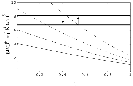
FIG. 1.: The BR for the decay $B^{\pm}\rightarrow\eta^{\prime}K^{\pm}$ vs $\xi$. The solid line is for the SM. The dashed, dotted and dot-dashed lines correspond to $|\lambda^{\prime}_{323}|=|\lambda^{\prime}_{322}|=0.04$, 0.06, 0.08, respectively. The bold solid lines indicate the experimental world average bound.

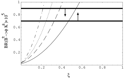
FIG. 2.: The BR for the deacy $B^{\pm}\rightarrow\phi K^{\pm}$ vs $\xi$. The solid line is for the SM. The dashed, dotted and dot-dashed lines correspond to $|\lambda^{\prime}_{323}|=|\lambda^{\prime}_{322}|=0.04$, 0.06, 0.08, respectively. The bold solid lines indicate the experimental world average bound.

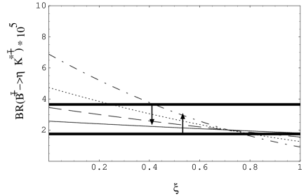
FIG. 3.: The BR for the deacy $B^{\pm}\rightarrow\eta K^{*\pm}$ vs $\xi$. The solid line is for the SM. The dashed, dotted and dot-dashed lines correspond to $|\lambda^{\prime}_{323}|=|\lambda^{\prime}_{322}|=0.04$, 0.06, 0.08, respectively. The bold solid lines indicate the experimental bound.

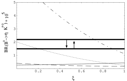
FIG. 4.: The BR for the deacy $B^{0}\rightarrow\eta K^{*0}$ vs $\xi$. The solid line is for the SM. The dashed, dotted and dot-dashed lines correspond to $|\lambda^{\prime}_{323}|=|\lambda^{\prime}_{322}|=0.04$, 0.06, 0.08, respectively. The bold solid lines indicate the experimental bound.

In Fig. 2, we plot the BR for the deacy $B^{\pm}\rightarrow\phi K^{\pm}$ for the same set of couplings. The observed BR of this mode by the CLEO [5] is (in $10^{-6}$) $5.5^{+2.1}_{-1.8}\pm 0.6$. The Belle and the BaBar collaboration have also observed this mode [8, 11] with BRs (in $10^{-6}$) $11.2^{+2.2}_{-2.0}\pm 1.4$ and $7.7^{+1.6}_{-1.4}\pm 0.8$, respectively. From the figure we see that the BR is increasing with $|\lambda^{\prime}|$. The BR for $|\lambda^{\prime}_{323}|=|\lambda^{\prime}_{322}|=0.06$ and $\xi\simeq 0.25-0.3$ is consistent with the world average bound $(7-9)\times 10^{-6}$. Now combining Fig. 1 and Fig. 2, we find that $|\lambda^{\prime}_{323}|=|\lambda^{\prime}_{322}|=0.06$ is allowed by both decay modes for $\xi\sim 0.25$. We note that the BaBar’s number for this mode is quite close to the value observed by the CLEO, but the Belle’s number is more than 2$\sigma$ away from the CLEO’s central value. We hope that this discrepancy will be sorted out in the near future.

In Fig. 3, we exhibit the BR for the deacy $B^{\pm}\rightarrow\eta K^{*\pm}$ as a function of $\xi$. The observed BR of this mode [4] is ${\mathcal{B}}(B^{\pm}\rightarrow\eta K^{*\pm})\times 10^{-6}=26.4^{+9.6}_{-8.2}\pm 3.3$. We find that the solution we have got from our previous two decay modes holds in this case: i.e., $|\lambda^{\prime}_{323}|=|\lambda^{\prime}_{322}|=0.06$ is allowed for $\xi\sim 0.15-0.25$.

Since all the parameters are fixed, now it is interesting to see whether the decay $B^{0}\rightarrow\eta K^{*0}$ fits in the allowed region. The observed BR for this mode by CLEO collaboration [4] is (in $10^{-6}$) $13.8^{+5.5}_{-4.6}\pm 1.6$. The Belle and the BaBar collaboration have also observed this mode [8, 10] with BRs (in $10^{-6}$) $19.8^{+6.5}_{-5.6}\pm 1.7$ and $21.2^{+5.4}_{-4.7}\pm 2.0$, respectively. The SM BR is very small and cannot explain the experimental data. In Fig. 4, we plot $B^{0}\rightarrow\eta K^{*0}$, where the world average value of the data is expressed as the bold solid line. We find that the dotted line ($|\lambda^{\prime}|=0.06$) is allowed for $\xi\lesssim 0.2$. But, the estimated BR for $|\lambda^{\prime}_{323}|=|\lambda^{\prime}_{322}|=0.06$ at $\xi\simeq 0.25$ is just below and very close to the lower bound of the average data. In fact, $|\lambda^{\prime}_{323}|=|\lambda^{\prime}_{322}|=0.06$ is allowed by both the CLEO and the Belle data for $\xi\lesssim 0.25$. Only the BaBar’s number is a little bit larger than our estimated BR at $0.2<\xi\lesssim 0.25$.

There exists a result for another decay mode involving $\eta^{\prime}$, i.e., $B^{0}\rightarrow\eta^{\prime}K^{0}$. For $|\lambda^{\prime}|=0.06$ and $\xi=0.25$ we find the BR is $88.3\times 10^{-6}$. The CLEO bound is (in $10^{-6}$) $89^{+18}_{-16}\pm 9$. The Belle and the BaBar collaboration also have reported observation of this mode but with less significance, and their results are (in $10^{-6}$) $55^{+19}_{-16}\pm 8$ and $42^{+13}_{-12}\pm 4$, respectively. We see that the results for this mode from the three experiments are not consistent. Our result in this scenario can be taken as a prediction which is in agreement with the CLEO result.

TABLE I.: The branching ratios $({\mathcal{B}})$ for $B$ decays into $PP$ and $VP$ final states at $\xi=0.25$.

Decay modes	${\mathcal{B}}$ $(10^{-6})$	${\mathcal{B}}$ $(10^{-6})$	Experimental ${\mathcal{B}}$ $(10^{-6})$
	$\gamma=110^{0}$	$\gamma=80^{0}$
$B^{0}\rightarrow\pi^{+}\pi^{-}$	5.96	6.0	$4.3^{+1.6}_{-1.4}\pm 0.5$ (CLEO[1]), $5^{+2.3+0.4}_{-2.0-0.5}$ (Belle[6])
			$4.1\pm 1\pm 0.7$ (BaBar[9])
$B^{+}\rightarrow K^{+}\pi^{0}$	9.59	9.19	$11.6^{+3.0+1.4}_{-2.7-1.3}$[1], $16.3^{+3.5+1.6}_{-3.3-1.8}$ [6]
			$10.8^{+2.1}_{-1.9}\pm 1.0$[9]
$B^{+}\rightarrow K^{0}\pi^{+}$	13.6	15.63	$18.2^{+4.6}_{-4.0}\pm 1.6$[1], $13.7^{+5.7+1.9}_{-4.8-1.8}$ [6]
			$18.2^{+3.3}_{-3.0}\pm 2.0$[9]
$B^{0}\rightarrow K^{+}\pi^{-}$	15.10	14.50	$17.2^{+2.5}_{-2.4}\pm 1.2$[1], $19.3^{+3.4+1.5}_{-3.2-0.6}$ [6]
			$16.7\pm 1.6\pm 1.3$[9]
$B^{0}\rightarrow K^{0}\pi^{0}$	8.68	9.87	$14.6^{+5.9+2.4}_{-5.1-3.3}$[1], $16.0^{+7.2+2.5}_{-5.9-2.7}$ [6]
			$8.2^{+3.1}_{-2.7}\pm 1.2$[9]
$B^{+}\rightarrow\omega\pi^{+}$	9.518	9.0	$11.3^{+3.3}_{-2.9}\pm 1.5$ (CLEO[2]), $6.6^{+2.1}_{-1.8}\pm 0.7$(BaBar[10])
$B^{+}\rightarrow\rho^{0}\pi^{+}$	9.418	9.45	$10.4^{+3.3}_{-3.4}\pm 2.1$[2], $24\pm 8\pm 3$[10]
$B^{0}\rightarrow\rho^{\mp}\pi^{\pm}$ (sum)	35.23	35.03	$27.6^{+8.4}_{-7.4}\pm 4.2$[2]
$B^{+}\rightarrow\omega h$	10.87	12.18	$14.3^{+3.6+2.1}_{-3.2-2.1}$ (CLEO[3])
$B^{0}\rightarrow K^{*+}\pi^{-}$	5.93	4.15	$22^{+8+4}_{-6-5}$[3]

The ${\cal B}(B\rightarrow X_{s}\nu\nu)$ can put bound on $\lambda^{\prime}_{322}\lambda^{\prime\ast}_{323}$ in certain limits. Using the Refs. [26] and the experimental limit (BR$<6.4\times 10^{-4}$) on the above BR [27], we find that $\lambda^{\prime}\leq 0.07$. However, if we go to any realistic scenario, for example grand unified models (with $R$ parity violation), we find a natural hierarchy among the sneutrino and squark masses. The squark masses are much heavier than the sneutrino masses and the bound does not apply any more.

The other observed $B\rightarrow PP$ and $B\rightarrow VP$ decay modes are listed in Table I for $\xi=0.25$ and we find that the BRs are within the experimental limits. Our result on $B^{0}\rightarrow K^{*+}\pi^{-}$ is compatible within 2$\sigma$ range, but this measurement still involves large error.

We can use smaller value of $\gamma$, e.g., $\gamma=80^{0}$ to fit the $B\rightarrow\eta^{(\prime)}K^{(*)}$ data. In this scenario we use $m_{s}~{}({\rm at}~{}m_{b}~{}{\rm scale})=75$ MeV. In Table II we show the BRs for $B\rightarrow\eta^{(\prime)}K^{(*)}$ and in Table I we show the BRs for the other observed $B\rightarrow PP$ and $B\rightarrow VP$ decay modes in the case of $\gamma=80^{0}$. Again, we find the fit is reasonable. In this case, we use $A_{0}^{B\rightarrow K^{*}}=0.4$ and keep the other inputs unchanged.

TABLE II.: The branching ratios $({\cal B})$ and the CP asymmetries for $B\rightarrow\eta^{(\prime)}K^{(*)}$ and $B\rightarrow\phi K$.

	$\delta=0$,		$\delta=15^{0}$		$\delta=0$,		$\delta=55^{0}$
	$\gamma=110^{0}$,		$\gamma=110^{0}$		$\gamma=80^{0}$,		$\gamma=80^{0}$
mode	${\cal B}\times 10^{6}$	${\cal A}_{CP}$	${\cal B}\times 10^{6}$	${\cal A}_{CP}$	${\cal B}\times 10^{6}$	${\cal A}_{CP}$	${\cal B}\times 10^{6}$	${\cal A}_{CP}$
$B^{+}\to\eta^{\prime}K^{+}$	68.9	0.01	68.3	0.04	82.1	0.01	68.3	0.11
$B^{+}\to\eta K^{*+}$	36.4	0.03	36.4	0.04	36.5	0.03	32.7	0.09
$B^{0}\to\eta^{\prime}K^{0}$	88.3	0.00	86.8	0.03	110.2	0.00	87.1	0.12
$B^{0}\to\eta K^{*0}$	14.0	$-0.39$	14.6	$-0.42$	14.8	$-0.28$	20.4	$-0.56$
$B^{+}\to\phi K^{+}$	7.11	0.00	6.97	0.04	7.10	0.00	5.76	0.14

We now calculate the CP asymmetry for different $B\rightarrow\eta^{(\prime)}K^{(*)}$ modes. The CP asymmetry, ${\mathcal{A}}_{CP}$, is defined by

$${\mathcal{A}}_{CP}={{\mathcal{B}}(B\rightarrow f)-{\mathcal{B}}(\overline{B}\rightarrow\bar{f})\over{\mathcal{B}}(B\rightarrow f)+{\mathcal{B}}(\overline{B}\rightarrow\bar{f})}~{},$$ (16)

where $B$ and $f$ denote a $B$ meson and a generic final state, respectively. Let us define

$$\lambda^{\prime}_{323}\lambda^{\prime\ast}_{322}=|\lambda^{\prime}_{323}\lambda^{\prime\ast}_{322}|e^{i\delta},$$ (17)

where $\delta$ denotes the phase difference between $\lambda_{323}^{\prime}$ and $\lambda_{322}^{\prime}$. So far we have discussed the $\delta=0^{0}$ situation. In Table II, we calculate the CP asymmetries for $B\rightarrow\eta K$ modes for different values of $\delta$ and $\gamma$. The maximum values of $\delta$ allowed by the BR of $B^{\pm}\rightarrow\eta^{\prime}K^{\pm}$ are $\delta=15^{0}$ for $\gamma=110^{0}$ and $\delta=55^{0}$ for $\gamma=80^{0}$. We find that ${\cal A}_{CP}$ is very large for $B^{0}\to\eta K^{*0}$ mode and is predicted to be $-39\%~{}(-42\%)$ for $\delta=0^{0}~{}(15^{0})$, $\gamma=110^{0}$, and $-28\%~{}(-56\%)$ for $\delta=0^{0}~{}(55^{0})$, $\gamma=80^{0}$. ${\cal A}_{CP}$ for $B^{\pm}\rightarrow\phi K^{\pm}$ is large ($14\%$) for $\delta=55^{0}$ and $\gamma=80^{0}$. The other $\eta^{(\prime)}$ modes are also found to be large ($\sim 10\%$) for the above set of parameters.

Case 2: We use the same form factors as in the case $\gamma=80^{0}$ of Case 1 and we use $m_{s}~{}({\rm at}~{}m_{b}~{}{\rm scale})=85$ MeV and $\gamma=110^{0}$. We now use the combination of $d^{R}_{222}$ and $d^{L}_{222}$. We assume $d^{R}_{222}=-d^{L}_{222}$. In this scenario, the $R_{p}\!\!\!\!\!\!/~{}~{}$ coupling part of the amplitude in $B\rightarrow\phi K$ decay mode canceled exactly (Eq. 10). (In fact, our solution still works when the cancellation is incomplete by about 5$\%$.) But we still have contributions to $B^{\pm}\rightarrow\eta^{\prime}K^{\pm}$ (Eq. 9) and to increase the BR we choose $d^{R}_{222}$ to be positive. There is no $R_{p}\!\!\!\!\!\!/~{}~{}$ contribution to the other $B\rightarrow PP$ and $B\rightarrow VP$ modes in this case as well.

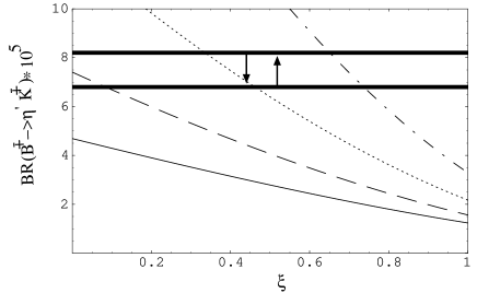
FIG. 5.: The BR for the deacy $B^{\pm}\rightarrow\eta^{\prime}K^{\pm}$ vs $\xi$. The solid line is for the SM. The dashed, dotted and dot-dashed lines correspond to $|\lambda^{\prime}|=0.035$, 0.052, 0.07, respectively. The bold solid lines indicate the experimental bound.

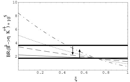
FIG. 6.: The BR for the deacy $B^{\pm}\rightarrow\eta K^{*\pm}$ vs $\xi$. The solid line is for the SM. The dashed, dotted and dot-dashed lines correspond to $|\lambda^{\prime}|=0.035$, 0.052, 0.07, respectively. The bold solid lines indicate the experimental bound.

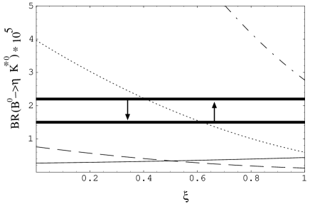
FIG. 7.: The BR for the deacy $B^{0}\rightarrow\eta K^{*0}$ vs $\xi$. The solid line is for the SM. The dashed, dotted and dot-dashed lines correspond to $|\lambda^{\prime}|=0.035$, 0.052, 0.07, respectively. The bold solid lines indicate the experimental bound.

In Fig. 5, we plot the BR for the deacy $B^{\pm}\rightarrow\eta^{\prime}K^{\pm}$ as a function of $\xi$. We have used $|\lambda^{\prime}|=0.035$, 0.052, 0.07, and $m_{\rm susy}=200$ GeV. In this case, the large branching ratio can be explained for $\lambda^{\prime}\geq 0.05$.

In Fig. 6 and Fig. 7, we plot the BRs for $B^{\pm}\rightarrow\eta K^{*\pm}$ and $B^{0}\rightarrow\eta K^{*0}$. Combining Figs. 5, 6 and 7, we find that $|\lambda^{\prime}|$=0.052 and $\xi\simeq 0.4-0.6$ can explain all the data. In this scenario our result on $B^{0}\to\eta K^{*0}$ is allowed by the world average bound. The BR of $B^{0}\rightarrow\eta^{\prime}K^{0}$ is $107.4\times 10^{-6}$ for $|\lambda^{\prime}|=0.052$ and $\xi=0.45$ and is allowed by the CLEO data.

The BR for the deacy $B^{\pm}\rightarrow\phi K^{\pm}$ does not have a $R_{p}\!\!\!\!\!\!/~{}~{}$ contribution due to the cancellation. The SM line (solid) in Fig. 2 needs to be used in this case and we find that $\xi\simeq 0.45$ is allowed. The BRs of the other observed $B\rightarrow PP$ and $B\rightarrow VP$ modes do not get affected by the new couplings and these modes seem to fit the data reasonably well for $\xi\simeq 0.3-0.5$ [16]. We also calculate the ${\cal A}_{CP}$ for this case. Since we have assumed that $d^{R}_{222}=-d^{L}_{222}$, the phase difference between $\lambda^{\prime}_{322}$ and $\lambda^{\prime}_{332}$ is ($\delta+\pi$), where $\delta$ is the phase difference between $\lambda^{\prime}_{323}$ and $\lambda^{\prime}_{322}$.

TABLE III.: The branching ratios $({\cal B})$ and the CP asymmetries for $B\rightarrow\eta^{(\prime)}K^{(*)}$ and $B\rightarrow\phi K$.

	$\delta=0$		$\delta=20^{0}$
mode	${\cal B}\times 10^{6}$	${\cal A}_{CP}$	${\cal B}\times 10^{6}$	${\cal A}_{CP}$
$B^{+}\to\eta^{\prime}K^{+}$	69.3	0.01	68.0	0.05
$B^{+}\to\eta K^{*+}$	27.9	0.04	27.8	0.05
$B^{0}\to\eta^{\prime}K^{0}$	107.4	0.00	104.5	0.05
$B^{0}\to\eta K^{*0}$	20.5	$-0.71$	21.1	$-0.72$
$B^{+}\to\phi K^{+}$	6.56	0.00	6.56	0.00

In Table III, we calculate the BRs and the CP asymmetries for $B\rightarrow\eta^{(\prime)}K^{(*)}$ and $B\rightarrow\phi K$ for different values of $\delta$. The maximum value of $\delta$ allowed by the BR for $B^{\pm}\rightarrow\eta^{\prime}K^{\pm}$ is $\delta=20^{0}$ for $\gamma=110^{0}$. As in $\bf Case1$, we find that ${\cal A}_{CP}$ is very large for $B^{0}\to\eta K^{*0}$ mode and is predicted to be $-71\%~{}(-72\%)$ for $\delta=0^{0}~{}(20^{0})$. The other $\eta^{(\prime)}$ modes are found to be $\sim 5\%$ for the above set of parameters.

V Conclusion

We have studied $B\rightarrow\eta^{(\prime)}K^{(*)}$ modes in the context of $R_{p}\!\!\!\!\!\!/~{}~{}$ supersymmetric theories. We have isolated the necessary $R_{p}\!\!\!\!\!\!/~{}~{}$ couplings ($\lambda^{\prime}_{323}\lambda^{\prime*}_{322}$ and $\lambda^{\prime}_{322}\lambda^{\prime*}_{332}$) that satisfy the experimental results for the BRs of these modes reasonably well. The Standard Model contribution is less than $2\sigma$ for some of these modes. These new couplings do not affect any other $B\rightarrow PP$ and $B\rightarrow VP$ modes except for the decay $B^{\pm}\rightarrow\phi K^{\pm}$. We have shown that the calculated BR for $B^{\pm}\rightarrow\phi K^{\pm}$ agrees with the experimental data.

We found solutions for both large and small values of $\gamma=110^{0},\,80^{0}$ and two different values of $\xi(=1/N_{c})\simeq 0.25,\,0.45$ for two different scenarios. For our solutions, we need $|\lambda^{\prime}|\sim 0.05-0.06$ for $m_{\rm susy}=200$ GeV. Using these preferred values of the parameters, we calculated the CP asymmetry of different observed modes affected by the new couplings and found that the CP asymmetry of $B^{0}\to\eta K^{*0}$ is large ($\sim 28\%-72\%$) and the CP asymmetry of other modes also can be around $10-15\%$.

These new coupling can be also examined in the RUN II through the associated production of the lightest chargino ($\chi^{\pm}_{1}$) and the second lightest neutralino ($\chi^{0}_{2}$). $\chi^{\pm}_{1}$ and $\chi^{0}_{2}$ decay into lepton plus 2 jets (for example), where one of the jets is a $b$ jet. The final state of this production process contains 2 leptons plus 4 jets. So the signal is quite interesting and unique.

ACKNOWLEDGMENTS

The work of C.S.K. was supported in part by CHEP-SRC Program, Grant No. 20015-111-02-2 and Grant No. R03-2001-00010 of the KOSEF, in part by BK21 Program and Grant No. 2001-042-D00022 of the KRF, and in part by Yonsei Research Fund, Project No. 2001-1-0057. The work of B.D. was supported in part by National Science Foundation grant No. PHY-0070964. The work of S.O. was supported by Grant No. 2001-042-D00022 of the KRF.

REFERENCES

[1]D. Cronin-Hennessy et al. (CLEO collaboration), Phys. Rev. Lett 85, 515 (2000).
[2]C.P. Jessop et al. (CLEO collaboration), Phys. Rev. Lett 85, 2881 (2000).
[3]M. Bishai et al. (CLEO collaboration), CLEO-Conf 99-13,
hep-ex/9908018.
[4]S.J. Richichi et al. (CLEO collaboration), Phys. Rev. Lett 85, 520 (2000).
[5]R.A. Brieri et al. (CLEO collaboration), Phys. Rev. Lett 86,
3718 (2001).
[6]K. Abe et al. (Belle collaboration), Phys. Rev. Lett. 87,
1081 (2001).
[7]K. Abe et al. (Belle collaboration), Phys. Lett. B517,
309 (2000).
[9]B. Aubert et al. (BaBar collaboration), Phys. Rev. Lett. 87,
151802 (2001).
[10]B. Aubert et al. (BaBar collaboration), SLAC-PUB-8981,
hep-ex/01070378.
[11]B. Aubert et al. (BaBar collaboration), Phys. Rev. Lett. 87,
151801 (2001).
[12]B. Aubert et al. (BaBar collaboration), Phys. Rev. Lett. 87,
221802 (2001).
[13]D.K. Ghosh, X-G. He, B.H.J. McKellar, J-Q. Shi,
hep-ph/0111106; G. Bhattacharyya, A. Datta and
A. Kundu, Phys. Lett. B514, 47 (2001); K. Huitu, D.X. Zhang,
C.D. Lu and P. Singer, Phys. Rev. Lett. 81, 4313 (1998);
C-h. Chang and T.-f. Feng, hep-ph/9908295; Eur. Phys. J. C12, 137 (2000);
D. Guetta, Phys. Rev. D58, 116008 (1998).
[14]D. Choudhury, B. Dutta and A. Kundu, Phys. Lett. B456,
185(1999).
[15]H.-Y. Cheng and K.-C. Yang, Phys. Rev. D62, 054029 (2000).
[16]B. Dutta and S. Oh, Phys. Rev. D63, 054016 (2001).
[17] A.J. Buras et al., Nucl. Phys. B400, 37 (1993); A.J. Buras,
M. Jamin and M.E. Lautenbacher, ibid. B400, 75 (1993).
[18] M. Ciuchini et al., Nucl. Phys. B415, 403, (1994).
[19] N.G. Deshpande, B. Dutta and S. Oh, Phys. Rev. D57, 5723 (1998);
N. G. Deshpande, B. Dutta and S. Oh, Phys. Lett. B473, 141 (2000).
[20] A. Ali, G. Kramer, C.-D. Lu, Phys. Rev. D58, 094009 (1998).
[21] I.-H. Lee, Phys. Lett. B138, 121 (1984); Nucl. Phys.
B246, 120 (1984); F. de Campos et al., Nucl. Phys. B451, 3 (1995);
M.A. Diaz, Univ. of Valencia report no. IFIC-98-11 (1998), hep-ph/9802407, and
references therein; S. Roy and B. Mukhopadhyaya, Phys. Rev. D55, 7020,
(1996).
[22] V. Barger, G.F. Giudice and T. Han, Phys. Rev. D40,
2987 (1989); G. Bhattacharyya and D. Choudhury, Mod. Phys. Lett. 10, 1669
(1995); M. Hirsch, H.V. Klapdor-Kleingrothaus and S.G. Kovalenko, Phys. Rev.
Lett. 75, 17 (1995); K.S. Babu and R.N.Mohapatra, Phys. Rev. Lett.
75, 2276 (1995).
[23] C.E. Carlson, P. Roy and M. Sher, Phys. Lett. B357, 94
(1995); K. Agashe and M. Graesser, Phys. Rev. D54, 4445 (1996); A.Y.
Smirnov and F. Vissani, Phys. Lett. B380, 317 (1996); D. Choudhury and P.
Roy, Phys. Lett. B378, 153 (1996).
[24] H. Dreiner, in ‘Perspectives on Supersymmetry’, ed. G.L. Kane
(World Scientific), hep-ph/9707435;
G. Bhattacharyya, hep-ph/9709395.
[25]
P. Ball, J.M. Frère and M. Tytgat, Phys Lett. B365, 367 (1996);
For a different parametrization of the mixing, see
T. Feldmann, P. Kroll and B. Stech, Phys. Rev. D58, 114006 (1998);
T. Feldmann, Int. J. Mod. Phys. A15, 159 (2000).
[26]Y. Grossman and Z. Ligeti, Nucl. Phys. B465, 369 (1996);
Erratum-ibid. B480, 753 (1996).
[27] R. Barate etal, ALEPH collaboration, Eur. Phys. J. C19,
213 (2001).