Electromagnetic Form Factors of Nucleons in a Light-cone Diquark Model

Abstract

We investigate the electromagnetic form factors of nucleons within a simple relativistic quark spectator-diquark model using the light-cone formalism. Melosh rotations are applied to both quark and vector diquark. It is shown that the difference between vector and scalar spectator diquarks reproduces the right electric form factor of neutrons, and both the form factors $G_{E}\left(Q^{2}\right)$ and $G_{M}\left(Q^{2}\right)$ of the proton and neutron agree with experimental data well up to $Q^{2}=2~{}\rm{GeV}^{2}$ in this simple model.

I Introduction

Since the photon is a particularly clean probe, the electromagnetic interactions are unique tools for investigating hadronic physics. Different electromagnetic processes are described by different transition form factors. For example, in the case of electron-nucleon elastic scattering processes, the Sachs form factors $G^{N}_{E}$ (electric) and $G^{N}_{M}$ (magnetic) contain all the information. At low momentum transfers, $G^{N}_{E}$ and $G^{N}_{M}$ are related to the spatial Fourier transform of the nucleon’s charge and magnetization distributions; while at high momentum transfers, these form factors give important information about the quark structure within the nucleon and also about the short-range behavior of the strong interactions. In fact, precise knowledge of the elastic electromagnetic form factors not only discloses the internal substructure of nucleons, but is also important for other processes, such as the experimental measurement of nucleon strangeness form factors Muller et al. (1997) and also for the nucleon spin problemBrodsky (1994a).

Theoretically, the very high $Q^{2}$ behavior of the nucleon form factors can be well described by perturbative quantum chromodynamics (QCD) Brodsky (1980a). However, as QCD bound states, and due to the large coupling constant of QCD in the non-perturbative region, the nucleons have to be explored in phenomenological QCD models or in lattice QCD. The non-relativistic constituent quark model is quite successful in explaining the static properties of baryons, but with increasing transfer momentum, it must fail in explaining the nucleon form factors because the intrinsic momentum of the quarks within a nucleon has the same order of magnitude as the quark mass. Thus, recently, many studies of nucleon form factors have been extended to relativistic quark models Dong et al. (1999), and also to light-cone Schlumpf (1993); Cardarelli and Simula (1999) and point-form Wagenbrunn et al. (2001) models. These relativistic quark models partially solved the shortcomings of its non-relativistic counterparts.

The purpose of this work is to show that both the electric and magnetic form factors of the proton and neutron can be reproduced in a simple relativistic quark spectator-diquark model which is formulated in the light-cone frame. This model was originally proposed in order to study deep inelastic lepton nucleon scattering Close (1973), based on the quark-parton model picture Feynman (1969) that deep inelastic scattering is well described by the impulse approximation, in which the incident lepton scatters incoherently off a quark in the nucleon, with the remaining nucleon constituents treated as a quasi-particle spectator. After taking into account Melosh rotation effects, this model is in good agreement with the experimental data of polarized deep inelastic scattering, and the mass difference between the scalar and vector spectators reproduces the up and down valence quark asymmetry Ma (1991). In this work we extend the relativistic quark spectator-diquark model in order to investigate electron-nucleon elastic scattering processes, where the single quark is the struck constituent and the non-interacting diquark serves to provide the quantum numbers of the spectator system. Recently, a covariant quark-diquark model was proposed in order to describe the nucleon properties Oettel and a d L. von Smekal (2000), but it was not formulated in light-cone quantization. The light-cone Fock representation of composite systems has a number of remarkable properties. The matrix elements of local operators such as electromagnetic currents have exact representation in terms of light-cone wave functions of Fock states Brodsky et al. (2000). If one chooses the special frame Drell and Yan (1970) $q^{+}=0$ for the space-like momentum transfer and takes the matrix elements of plus components of currents, the contribution from pair creation or annihilation is forbidden and the matrix elements of space-like currents can be expressed as overlaps of light-cone wave functions with the same number of Fock constituents.

This paper is organized as follows. In section II, the relativistic quark-diquark model formulated in the light-cone frame is introduced. The specific light-cone form is obtained by transforming instant into light-cone states using Melosh rotations. The detailed matrix elements of electromagnetic currents are given in section III. In section IV, we present the results for the nucleon electromagnetic properties calculated in the light-cone diquark model. Finally, a brief summary is given in section V.

II The light-cone quark spectator-diquark model

The proton wave function in the conventional $SU\left(6\right)$ quark model is given by

$$\left.\left.\right|p^{\uparrow}\right\rangle=\frac{1}{\sqrt{18}}\left[\left(u^{\downarrow}d^{\uparrow}-u^{\uparrow}d^{\downarrow}\right)u^{\uparrow}+({\rm cyclic\;permutation})\right].$$ (1)

In the impulse approximation, the incident lepton strikes incoherently a single constituent quark in the nucleon, with the remain nucleon constituents treated as a quasi-particle spectator to provide the other quantum numbers of nucleons. Thus, it is more convenient to rewrite the wave function of the conventional $SU\left(6\right)$ quark model in the quark spectator-diquark form. In fact, in the quark spectator-diquark form, some non-perturbative effects between the two spectator quarks or other non-perturbative gluon effects in the nucleon can be effectively taken into account by the mass of the diquark spectator. Starting from Eq. (1), the proton wave function of the quark-diquark model in the instant form can be written as Ma (1991); Pavković (1976)

$$\Psi_{p}^{\uparrow,\downarrow}\left(qD\right)=\sin\theta\,\varphi_{V}\,\left.\left.\right|qV\right\rangle^{\uparrow,\downarrow}+\cos\theta\,\varphi_{S}\,\left.\left.\right|qS\right\rangle^{\uparrow,\downarrow},$$ (2)

with

$$\left.\left.\right|qV\right\rangle^{\uparrow,\downarrow} = \pm\frac{1}{3}\left[V^{0}\left(ud\right)u^{\uparrow,\downarrow}-\sqrt{2}V^{\pm 1}\left(ud\right)u^{\downarrow,\uparrow}-\sqrt{2}V^{0}\left(uu\right)d^{\uparrow,\downarrow}+2V^{\pm 1}\left(uu\right)d^{\downarrow,\uparrow}\right],$$

$$\left.\left.\right|qS\right\rangle^{\uparrow,\downarrow} = S\left(ud\right)u^{\uparrow,\downarrow},$$ (3)

where $\theta$ is the mixing angle that breaks SU(6) symmetry at $\theta\neq\pi/4$, $V^{s_{z}}(q_{1}q_{2})$ is the $q_{1}q_{2}$ instant form vector diquark Fock state with third spin component $s_{z}$, $S(ud)$ is the $ud$ scalar diquark Fock state, and $\varphi_{D}$ stands for the momentum space wave function of the quark-diquark, with $D$ representing the vector ($V$) or scalar ($S$) diquarks. In this paper we choose the $SU\left(6\right)$ symmetry case $\theta=\pi/4$. The neutron wave function can be obtained simply by exchanging the $u$ and $d$ quarks.

Since the light-cone Fock representation of composite systems has a number of remarkable properties, we will calculate the electromagnetic properties of nucleons in this formalism. The light-cone momentum space wave function of the quark-spectator is assumed to be a harmonic oscillator wave function (the Brodsky-Huang-Lepage (BHL) prescription Brodsky et al. (1981); Huang (1994))

$$\varphi_{D}\left(x,\bm{k}_{\perp}\right)=A_{D}exp\left\{-\frac{1}{8\beta_{D}^{2}}\left[\frac{m_{q}^{2}+\bm{k}_{\perp}^{2}}{x}+\frac{m_{D}^{2}+\bm{k}_{\perp}^{2}}{1-x}\right]\right\},$$ (4)

where $m_{q}$ and $m_{D}$ are the masses for the quark $q$ and spectator $D$ respectively, $x$ and ${\bm{k}}_{\perp}$ are the light-cone momentum fraction and internal transversal momentum of quarks respectively, and $\beta_{D}$ is the harmonic oscillator scale parameter.

The spin part of the light-cone wave functions of nucleons can be obtained by transforming instant into light-cone states using Melosh rotations. For a spin-$\frac{1}{2}$ particle, the Melosh transformations are known to be Melosh (1974)

$$\chi^{\uparrow}_{T} = w\left[\left(k^{+}+m\right)\chi^{\uparrow}_{F}-k^{R}\chi^{\downarrow}_{F}\right],$$

$$\chi^{\downarrow}_{T} = w\left[\left(k^{+}+m\right)\chi^{\downarrow}_{F}-k^{L}\chi^{\uparrow}_{F}\right],$$ (5)

where $\chi_{T}$ and $\chi_{F}$ are instant and light-cone spinors respectively, $w=\left[2k^{+}\left(k^{0}+m_{q}\right)\right]^{-\frac{1}{2}}$, $k^{R,L}=k^{1}\pm ik^{2}$, and $k^{+}=k^{0}+k^{3}$. In this work, for simplicity we treat the diquark as a point particle. The scalar diquark does not transform, since it has zero spin. For the spin-$1$ vector diquark, the Melosh transformations are given by Ahluwalia and Sawicki as Ahluwalia and Sawicki (1993)

$$V^{1}_{T} = w^{2}\left[\left(k^{+}+m\right)^{2}V^{1}_{F}-\sqrt{2}\left(k^{+}+m\right)k^{R}V^{0}_{F}+{k^{R}}^{2}V^{-1}_{F}\right],$$

$$V^{0}_{T} = w^{2}\left[\sqrt{2}\left(k^{+}+m\right)k^{L}V^{1}_{F}+2\left(\left(k^{0}+m\right)k^{+}-k^{R}k^{L}\right)V^{0}_{F}-\sqrt{2}\left(k^{+}+m\right)k^{R}V^{-1}_{F}\right],$$

$$V^{-1}_{T} = w^{2}\left[{k^{L}}^{2}V^{1}_{F}+\sqrt{2}\left(k^{+}+m\right)k^{L}V^{0}_{F}+\left(k^{+}+m\right)^{2}V^{-1}_{F}\right].$$ (6)

Here, $V_{T}$ and $V_{F}$ are the instant and light-cone spin-$1$ spinors respectively, which are constructed within the Weinberg-Soper formalism Weinberg (1964). Ahluwalia and Sawicki Ahluwalia and Sawicki (1993) used this formalism in order to construct explicit hadronic spinors for arbitrary spin in the light-cone form, and obtained general Melosh rotations for spinors of arbitrary spin. In the case of spin-$\frac{1}{2}$, these spinors are in agreement with the results of Lepage and Brodsky Brodsky (1980a), and also the Melosh rotations are the same as in Eq. (II), which were introduced originally by Melosh. The Melosh rotations for spin-$1$ particles have a similar form as Eq. (II), if the spin-$1$ particle is treated as a composite state of two spin-$\frac{1}{2}$ particles.

III The calculation of electromagnetic form factors

The nucleon Sachs form factors are defined as combinations of the Dirac and Pauli form factors Sachs (1962)

$$G_{E}^{N}\left(Q^{2}\right) = F_{1}^{N}\left(Q^{2}\right)-\frac{Q^{2}}{4M^{2}}F_{2}^{N}\left(Q^{2}\right),$$

$$G_{M}^{N}\left(Q^{2}\right) = F_{1}^{N}\left(Q^{2}\right)+F_{2}^{N}\left(Q^{2}\right).$$ (7)

As a spin-$\frac{1}{2}$ composite system, the nucleon has Dirac and Pauli form factors $F_{1}\left(Q^{2}\right)$ and $F_{2}\left(Q^{2}\right)$ defined by

$$\left\langle P^{\prime}\left|J^{\mu}\left(0\right)\right|P\right\rangle=\bar{u}\left(P^{\prime}\right)\left[F_{1}^{N}\left(Q^{2}\right)\gamma^{\mu}+F_{2}^{N}\left(Q^{2}\right)\frac{i\sigma^{\mu\nu}q_{\nu}}{2M}\right]u\left(P\right),$$ (8)

where $q^{\mu}=\left(P^{\prime}-P\right)^{\mu}$ is four-momentum transfer, $Q^{2}=-q^{2}$, and $u\left(P\right)$ is the nucleon spinor. In the light-cone formalism, it is well known that the Dirac and Pauli form factors are equal to the helicity-conserving and helicity-flip matrix elements of the plus component of electromagnetic current operators Brodsky and Drell (1980):

$$\left\langle P^{\prime},\uparrow\left|\frac{J^{+}\left(0\right)}{2P^{+}}\right|P,\uparrow\right\rangle = F_{1}^{N}\left(Q^{2}\right),$$

$$\left\langle P^{\prime},\uparrow\left|\frac{J^{+}\left(0\right)}{2P^{+}}\right|P,\downarrow\right\rangle = -(q_{1}-iq_{2})\frac{F_{2}^{N}\left(Q^{2}\right)}{2M}.$$ (9)

In the $Q^{2}\rightarrow 0$ limit, the nucleon magnetic form factor is just the magnetic moment of the nucleon:

$$\mu_{N}=G_{M}^{N}\left(0\right).$$ (10)

Other important static electromagnetic properties of nucleons are the charge and magnetic radii, which can be obtained via the $Q^{2}\rightarrow 0$ limit of the electromagnetic form factors as:

$$r_{EN}^{2} = -6\,\lim_{Q^{2}\rightarrow 0}\frac{dG_{E}^{N}\left(Q^{2}\right)}{dQ^{2}},$$

$$r_{MN}^{2} = -6\,\lim_{Q^{2}\rightarrow 0}\frac{1}{\mu_{N}}\frac{dG_{M}^{N}\left(Q^{2}\right)}{dQ^{2}}.$$ (11)

In these calculations, we choose the Drell-Yan assignment Drell and Yan (1970):

$$q = \left(q^{+},q^{-},\bm{q}_{\perp}\right)=\left(0,\frac{-q^{2}}{P^{+}},\bm{q}_{\perp}\right),$$

$$P = \left(P^{+},P^{-},\bm{P}_{\perp}\right)=\left(P^{+},\frac{M^{2}}{P^{+}},\bm{0}_{\perp}\right).$$ (12)

As pointed out in the introduction, the matrix elements of space-like currents can be expressed as overlaps of light-cone wave functions with the same number of Fock constituents. In particular, for the form factors we have

$$F_{1}^{N}\left(Q^{2}\right) = \sum_{a}\int\frac{d^{2}\bm{k}_{\perp}dx}{16\pi^{3}}\sum_{j}e_{j}\psi^{\uparrow\star}_{a}\left(x_{i},\bm{k}^{\prime}_{\perp i},\lambda_{i}\right)\psi^{\uparrow}_{a}\left(x_{i},\bm{k}_{\perp i},\lambda_{i}\right),$$

$$-q^{L}\frac{F_{2}^{N}\left(Q^{2}\right)}{2M} = \sum_{a}\int\frac{d^{2}\bm{k}_{\perp}dx}{16\pi^{3}}\sum_{j}e_{j}\psi^{\uparrow\star}_{a}\left(x_{i},\bm{k}^{\prime}_{\perp i},\lambda_{i}\right)\psi^{\downarrow}_{a}\left(x_{i},\bm{k}_{\perp i},\lambda_{i}\right),$$ (13)

where $e_{j}$ is the charge of struck constituents, $\psi_{a}\left(x_{i},\bm{k}_{\perp i},\lambda_{i}\right)$ is the light-cone Fock expansion wave function, and $\lambda_{i}$, $x_{i}$ and $\bm{k}_{\perp i}$ are the spin projections along the quantization direction, light-cone momentum fractions and relative momentum coordinates of the QCD constituents, respectively. Here, for the final state light-cone wave function, the relative momentum coordinates are

$$\bm{k}^{\prime}_{\perp i}=\bm{k}_{\perp i}+\left(1-x_{i}\right)\bm{q}_{\perp}$$ (14)

for the struck quark and

$$\bm{k}^{\prime}_{\perp i}=\bm{k}_{\perp i}-x_{i}\bm{q}_{\perp}$$ (15)

for each spectator. This treatment is similar to that for the pion form factor with a quark-antiquark pair as constituents in the light-cone formalism Ma (1993).

Thus, in terms of the wave functions Eqs. (2, II, II) and (II), it is easy to obtain the expressions for the Dirac and Pauli form factors in our light-cone quark model. Explicit expressions for the proton form factors are:

$$F_{1}^{p}\left(Q^{2}\right) = 3\int\frac{d^{2}k_{\perp}dx}{16\pi^{3}}\frac{2}{3}\cos^{2}\theta w^{\prime}_{q}w_{q}\left[\left(k^{\prime+}_{q}+m_{q}\right)\left(k^{+}_{q}+m_{q}\right)+k^{\prime L}_{\perp}k^{R}_{\perp}\right]\varphi_{S}\left(x,\bm{k}^{\prime}_{\perp}\right)\varphi_{S}\left(x,\bm{k}_{\perp}\right),$$

$$F_{2}^{p}\left(Q^{2}\right) = \frac{6M}{-q^{L}}\int\frac{d^{2}k_{\perp}dx}{16\pi^{3}}\frac{2}{3}\cos^{2}\theta w^{\prime}_{q}w_{q}\left[\left(k^{\prime+}_{q}+m_{q}\right)k^{L}_{\perp}-\left(k^{+}_{q}+m_{q}\right)k^{\prime L}_{\perp}\right]$$ (16)

$$\,\,\times\varphi_{S}\left(x,\bm{k}^{\prime}_{\perp}\right)\varphi_{S}\left(x,\bm{k}_{\perp}\right).$$

It is interesting to notice that in the proton case the contributions of the vector diquark cancel each other exactly due to the spin-flavor structure of the proton wave functions. In the case of neutrons, the expressions are similar, but the contributions of vector diquarks do not cancel. For completion, we also present them in the Appendix.

IV Results and discussions

In our model there are five parameters: the quark mass $m_{q}$, the scalar and vector diquark masses $m_{S}$ and $m_{V}$, and the harmonic oscillator scale parameter $\beta_{S}$ and $\beta_{V}$, which are fixed by six static electromagnetic properties: the charge radii, magnetic radii and magnetic moments of both proton and neutron. This is given in Table 1. As we already noticed, in the proton case the vector diquark contributions to the form factors cancel each other exactly. Therefore, the three static electromagnetic properties of protons can fix completely the quark mass and the parameters corresponding to the scalar diquark. The other parameters are fixed by the neutron static properties. We calculate the static electromagnetic properties and form factors of nucleons using three different sets of parameters in order to show their dependence on the difference between the scalar and vector diquarks. We find that the electromagnetic properties of neutrons, specially the charge radius, are sensitive to the values of the parameters. When the value of the vector diquark harmonic oscillator scale parameter is less than that of the scalar diquark, we obtain a much larger positive squared charge radius for the neutron, although the neutron magnetic moment is in good agreement with experiment. In our calculations, the quark mass $m_{q}=0.220\,{\rm GeV}$ is much less than that used in the non-relativistic quark model $(m_{q}\sim M_{N}/3=0.313\,{\rm GeV})$. This is due to the fact that although in the non-relativistic quark model the proton magnetic moment has a simple relation with the quark mass, $\mu_{p}=\frac{M_{N}}{m_{q}}\sim 3$, in relativistic quark models, for example our model, this relation is more complicated, and it depends on both the mass and the intrinsic momentum of quarks within the nucleon. In fact, the value of the quark mass used in our model is comparable with that used in other relativistic quark model Capstick and Keister (1986). The model parameters used here are slightly different from those used in previous calculations of valence quark distributions, but these previous results are not sensitive to the actual values of the parameters and therefore the present parameters will give similar results.

The static electromagnetic properties of nucleons are shown in Table 2 for three different sets of parameters. In the first set we use the same mass and scale parameters for the scalar and vector diquarks in order to keep the $SU\left(6\right)$ symmetry of nucleon wave functions, but get nearly zero charge radius for the neutron and also the proton anomalous magnetic is close to that of the neutron. This choice of parameters is compatible with the naive $SU\left(6\right)$ symmetric quark model. However, the experimental negative squared charge radius of neutrons as well as the ratio $\mu_{p}/\mu_{n}=-1.46$ indicate that the $SU\left(6\right)$ symmetry is broken. In our model the $SU\left(6\right)$ breaking effect is introduced by the difference between the scalar and vector diquarks parameters, as it is shown with the third set of parameters. Except for the fact that the neutron magnetic moment is slightly off, the results of set III are in good agreement with experiment, through the difference between the scalar and vector diquarks parameters, which breaks the $SU\left(6\right)$ symmetry and gives the right neutron charge radius. Although the Melosh rotations already break the $SU\left(6\right)$ symmetry of nucleon wave functions, it is not enough to produce the right neutron charge radius Cardarelli and Simula (1999). In set II, we try to fix the neutron magnetic moment. However, we obtain a bad result for the neutron charge radius.

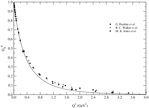
Figure 1: Electric form factor of protons. The experimental data are from Hoehler et al. (1976); Walker et al. (1994); Jones et al. (2000)

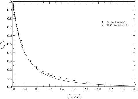
Figure 2: Magnetic form factor of protons. The experimental data are from Hoehler et al. (1976); Walker et al. (1994).

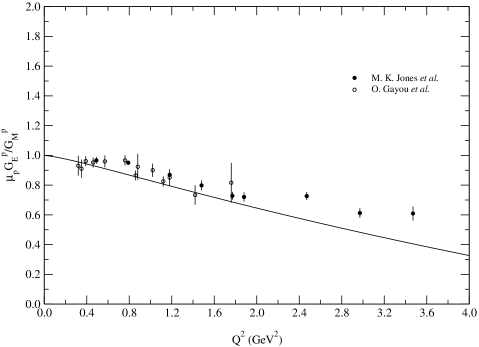
Figure 3: The ratio $\left(\mu_{p}G_{E}/G_{M}\right)$ of protons compared with the data from ref. Jones et al. (2000).

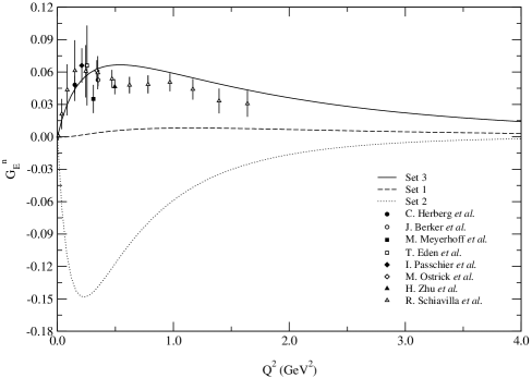
Figure 4: Electric form factor of neutrons. The experimental data are from Meyerhoff et al. (1994).

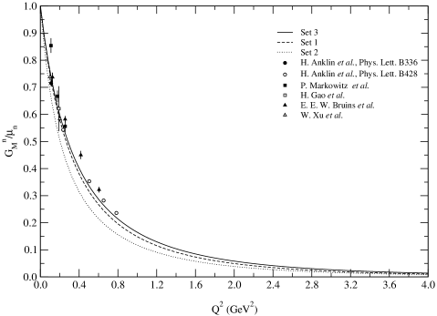
Figure 5: Magnetic form factor of neutrons. The experimental data are from Anklin et al. (1994).

In Figs. 1 and 2 we show the electromagnetic form factors of protons up to $Q^{2}=4\,{\rm GeV}^{2}$. Since as pointed out in Ref. Jones et al. (2000) the results for the electric form factor of protons from Ref. Hoehler et al. (1976); Walker et al. (1994) are too high, in Fig  1 we also present the results from Ref. Jones et al. (2000) for $G_{E}^{p}$, which are obtained by assuming that the proton magnetic form factor $G_{M}^{p}/\mu_{p}$ satisfies a dipole behaviour $G_{D}=1/\left[1+Q^{2}/0.71\right]^{2}$. Both form factors are in good agreement with experiment even up to $Q^{2}=4\,{\rm GeV}^{2}$. However, because of the harmonic oscillator wave functions used in our calculations, it is important to keep in mind that we expect our model to be valid essentially for $Q^{2}$ up to $2\,{\rm GeV}^{2}$. Recently, the JLab data Jones et al. (2000) showed that the $Q^{2}$ dependence of $G_{E}^{p}$ and of $G_{M}^{p}$ is significantly different, in contrast to the non-relativistic quark model prediction, in which both have the same behavior. In the light-cone frame, however, after taking into account the Melosh rotations, the $Q^{2}$ dependence is naturally different because the Dirac form factor is obtained from the helicity-conserving matrix element of the plus component of electromagnetic current operator while the Pauli form factor is obtained from the helicity-flip matrix element. Our results for the ratio between $G_{E}^{p}$ and $G_{M}^{p}$, together with the JLab data, are shown in Fig. 3, and the neutron electromagnetic form factors are shown in Figs. 4 and 5. In contrast to the proton case, the experimental data for the neutron has fewer points, and our results also agree with the available experimental data. Once again it is the difference between the scalar and vector diquarks which breaks the $SU\left(6\right)$ symmetry and reproduces the non-zero neutron electromagnetic form factor.

V summary

We have calculated the electromagnetic form factors of nucleons in a simple quark spectator-diquark model which is formulated in the light-cone formalism. The wave functions of the model are obtained by transforming the instant states into the light-cone states using Melosh rotations which are applied to both the quark and vector diquark. The model parameters are fixed by the six static electromagnetic properties of nucleons. We find that the calculated form factors are in good agreement with the experimental data, and that the ratio between the electric and magnetic form factors of protons also agrees with recent JLab data. The difference between the scalar and vector diquarks breaks the $SU\left(6\right)$ symmetry of the nucleon wave functions and it is essential in order to reproduce the correct electromagnetic nucleon properties. This framework is certainly applicable to calculate other processes such as nucleon-delta transitions and nucleon axial form factors, and would therefore be interesting to extend and check it in its application to these processes and also to reactions involving other baryons.

Appendix A

Using Eqs. (2,II,II, II) and (III), we obtain the explicit expressions of neutron form factors as:

$$F_{1}^{n}\left(Q^{2}\right) = 3\int\frac{d^{2}k_{\perp}dx}{16\pi^{3}}w^{\prime}_{q}w_{q}\left\{\frac{1}{9}\sin^{2}\theta\left\{\left[\left(k^{\prime+}_{q}+m_{q}\right)\left(k^{+}_{q}+m_{q}\right)+k^{\prime L}_{\perp}k^{R}_{\perp}\right]O_{V^{0,0}}\right.\right.$$ (17)

$$-\left.\left.\sqrt{2}\left[\left(k^{\prime+}_{q}+m_{q}\right)k^{L}_{\perp}-\left(k^{+}_{q}+m_{q}\right)k^{\prime L}_{\perp}\right]O_{V^{0,1}}\right.\right.$$

$$-\left.\left.\sqrt{2}\left[\left(k^{+}_{q}+m_{q}\right)k^{\prime R}_{\perp}-\left(k^{\prime+}_{q}+m_{q}\right)k^{R}_{\perp}\right]O_{V^{1,0}}\right.\right.$$

$$+\left.\left.2\left[\left(k^{\prime+}_{q}+m_{q}\right)\left(k^{+}_{q}+m_{q}\right)+k^{\prime R}_{\perp}k^{L}_{\perp}\right]O_{V^{1,1}}\right\}\varphi_{V}\left(x,\bm{k}^{\prime}_{\perp}\right)\varphi_{V}\left(x,\bm{k}_{\perp}\right)\right.$$

$$\left.-\frac{1}{3}\cos^{2}\theta\left[\left(k^{\prime+}_{q}+m_{q}\right)\left(k^{+}_{q}+m_{q}\right)+k^{\prime L}_{\perp}k^{R}_{\perp}\right]\varphi_{S}\left(x,\bm{k}^{\prime}_{\perp}\right)\varphi_{S}\left(x,\bm{k}_{\perp}\right)\right\},$$

and

$$F_{2}^{n}\left(Q^{2}\right) = \frac{6M}{-q^{L}}\int\frac{d^{2}k_{\perp}dx}{16\pi^{3}}w^{\prime}_{q}w_{q}\left\{-\frac{1}{9}\sin^{2}\theta\left\{\left[\left(k^{\prime+}_{q}+m_{q}\right)k^{L}_{\perp}-\left(k^{+}_{q}+m_{q}\right)k^{\prime L}_{\perp}\right]O_{V^{0,0}}\right.\right.$$ (18)

$$\left.\left.-\sqrt{2}\left[\left(k^{\prime+}_{q}+m_{q}\right)\left(k^{+}_{q}+m_{q}\right)+k^{\prime L}_{\perp}k^{R}_{\perp}\right]O_{V^{0,-1}}\right.\right.$$

$$\left.\left.-\sqrt{2}\left[\left(k^{\prime+}_{q}+m_{q}\right)\left(k^{+}_{q}+m_{q}\right)+k^{\prime R}_{\perp}k^{L}_{\perp}\right]O_{V^{1,0}}\right.\right.$$

$$\left.\left.+2\left[\left(k^{+}_{q}+m_{q}\right)k^{\prime R}_{\perp}-\left(k^{\prime+}_{q}+m_{q}\right)k^{R}_{\perp}\right]O_{V^{1,-1}}\right\}\varphi_{V}\left(x,\bm{k}^{\prime}_{\perp}\right)\varphi_{V}\left(x,\bm{k}_{\perp}\right)\right.$$

$$\left.-\frac{1}{3}\cos^{2}\theta\left[\left(k^{\prime+}_{q}+m_{q}\right)k^{L}_{\perp}-\left(k^{+}_{q}+m_{q}\right)k^{\prime L}_{\perp}\right]\varphi_{S}\left(x,\bm{k}^{\prime}_{\perp}\right)\varphi_{S}\left(x,\bm{k}_{\perp}\right)\right\},$$

where

$$O_{V^{0,0}} = {w^{\prime}}^{2}_{D}w^{2}_{D}\left[4\left(k^{\prime+}_{D}+m_{D}\right)\left(k^{+}_{D}+m_{D}\right){\bm{k}}^{\prime}_{\perp}\cdot{\bm{k}}_{\perp}+\left(\left(k^{\prime+}_{D}+m_{D}\right)^{2}-{{\bm{k}}^{\prime}}^{2}_{\perp}\right)\right.$$

$$\left.\times\left(\left(k^{+}_{D}+m_{D}\right)^{2}-{\bm{k}}^{2}_{\perp}\right)\right],$$

$$O_{V^{0,1}} = {w^{\prime}}^{2}_{D}w^{2}_{D}\left[-\sqrt{2}\left(k^{\prime+}_{D}+m_{D}\right)\left(k^{+}_{D}+m_{D}\right)^{2}k^{\prime R}_{\perp}+\sqrt{2}\left(\left(k^{\prime+}_{D}+m_{D}\right)^{2}-{{\bm{k}}^{\prime}}^{2}_{\perp}\right)\right.$$

$$\left.\times\left(k^{+}_{D}+m_{D}\right)k^{R}_{\perp}+\sqrt{2}\left(k^{\prime+}_{D}+m_{D}\right)k^{\prime L}_{\perp}{k^{R}_{\perp}}^{2}\right],$$

$$O_{V^{1,0}} = {w^{\prime}}^{2}_{D}w^{2}_{D}\left[-\sqrt{2}\left(k^{\prime+}_{D}+m_{D}\right)^{2}\left(k^{+}_{D}+m_{D}\right)k^{L}_{\perp}+\sqrt{2}\left(k^{\prime+}_{D}+m_{D}\right)\right.$$

$$\left.\times\left(\left(k^{+}_{D}+m_{D}\right)^{2}-{\bm{k}}^{2}_{\perp}\right)k^{\prime L}_{\perp}+\sqrt{2}\left(k^{+}_{D}+m_{D}\right){k^{\prime L}_{\perp}}^{2}k^{R}_{\perp}\right],$$

$$O_{V^{1,1}} = {w^{\prime}}^{2}_{D}w^{2}_{D}\left[\left(k^{\prime+}_{D}+m_{D}\right)^{2}\left(k^{+}_{D}+m_{D}\right)^{2}+2\left(k^{\prime+}_{D}+m_{D}\right)\left(k^{+}_{D}+m_{D}\right)\right.$$

$$\left.\times k^{\prime L}_{\perp}k^{R}_{\perp}+{k^{\prime L}_{\perp}}^{2}{k^{R}_{\perp}}^{2}\right],$$

$$O_{V^{0,-1}} = {w^{\prime}}^{2}_{D}w^{2}_{D}\left[-\sqrt{2}\left(k^{\prime+}_{D}+m_{D}\right)k^{\prime R}_{\perp}{k^{L}_{\perp}}^{2}-\sqrt{2}\left(\left(k^{\prime+}_{D}+m_{D}\right)^{2}-{{\bm{k}}^{\prime}}^{2}_{\perp}\right)\left(k^{+}_{D}+m_{D}\right)k^{L}_{\perp}\right.$$ (19)

$$\left.+\sqrt{2}\left(k^{\prime+}_{D}+m_{D}\right)\left(k^{+}_{D}+m_{D}\right)^{2}k^{\prime L}_{\perp}\right],$$

and

$$O_{V^{0,-1}} = {w^{\prime}}^{2}_{D}w^{2}_{D}\left[\left(k^{\prime+}_{D}+m_{D}\right)^{2}{k^{L}_{\perp}}^{2}-2\left(k^{\prime+}_{D}+m_{D}\right)\left(k^{+}_{D}+m_{D}\right)\right.$$ (20)

$$\left.\times k^{\prime L}_{\perp}k^{L}_{\perp}+\left(k^{+}_{D}+m_{D}\right)^{2}{k^{\prime L}_{\perp}}^{2}\right]$$

come from the Melosh rotations of vector diquarks, in which the superscript $\left(i,j\right)$ of $V$ indicates the third spin component of initial and final state vector diquarks.

Table 1: The three sets of parameters used in the calculations.

	Set I	Set II	Set III
$m_{q}$ (GeV)	0.220	0.220	0.220
$m_{s}$ (GeV)	0.500	0.500	0.500
$m_{v}$ (GeV)	0.500	0.700	0.700
$\beta_{s}$ (GeV)	0.250	0.250	0.250
$\beta_{v}$ (GeV)	0.250	0.170	0.330

Table 2: The static electromagnetic properties of nucleons for the three sets of parameters.

	Set I	Set II	Set III	Experimental
$\left(r_{p}\right)_{el}\left({\rm fm}\right)$	0.864	0.864	0.864	0.883(14)Melnikov and van Ritbergen (2000),0.880(15)Rosenfelder (2000)
$\left(r^{2}_{n}\right)_{el}\left({\rm fm}^{2}\right)$	0.003	0.514	$-$0.110	$-$0.113(7)Kopecky et al. (1995)
$\left(r_{p}\right)_{mag}\left({\rm fm}\right)$	0.853	0.853	0.853	0.843(13)Hoehler et al. (1976)
$\left(r_{n}\right)_{mag}\left({\rm fm}\right)$	0.873	1.016	0.847	0.840(42)Hoehler et al. (1976)
$\mu_{p}$	2.797	2.797	2.797	2.793Groom et al. (2000)
$\mu_{n}$	$-$1.840	-1.903	-1.664	$-$1.913Groom et al. (2000)

References

- (1)
- Muller et al. (1997) B. Muller et al., Phys. Rev. Lett. 78, 3824 (1997); K. A. Aniol et al., ibid. 82, 1096 (1999); Phys. Lett. B 509, 211 (2001).
- Brodsky (1994a) S. J. Brodsky and F. Schlumpf, Phys. Lett. B 329, 111 (1994a).
- Brodsky (1980a) G. P. Lepage and S. J. Brodsky, Phys. Rev. D 22, 2157 (1980a); S. J. Brodsky, H.-C. Pauli, and S. S. Pinsky, Phys. Rep. 301, 299 (1998b).
- Dong et al. (1999) Y. B. Dong, K. Shimizu, A. Faessler, and A. J. Buchmann, Phys. Rev. C 60, 035203 (1999).
- Schlumpf (1993) F. Schlumpf, Phys. Rev. D 47, 4114 (1993); W. Konen and H. J. Weber, ibid. 41, 2201 (1990); S. Capstick and B. D. Keister, ibid. 51, 3598 (1995).
- Cardarelli and Simula (1999) F. Cardarelli and S. Simula, Phys. Lett. B 467, 1 (1999); Phys. Rev. C 62, 065201 (2000).
- Wagenbrunn et al. (2001) R. F. Wagenbrunn, S. Boffi, W. Klink, W. Plessas, and M. Radici, Phys. Lett. B 511, 33 (2001).
- Close (1973) F. E. Close, Phys. Lett. 43B, 422 (1973); R. D. Field and R. P. Feynman, Phys. Rev. D 15, 2590 (1977).
- Feynman (1969) R. P. Feynman, Phys. Rev. Lett. 23, 1415 (1969); J. D. Bjorken, Phys. Rev. 179, 1547 (1969); J. D. Bjorken and E. A. Paschos, ibid. 185, 1975 (1969).
- Ma (1991) B.-Q. Ma, J. Phys. G 17, L53 (1991); Phys. Lett. B 375, 320 (1996).
- Oettel and a d L. von Smekal (2000) M. Oettel and R. Alkofer, Eur. Phys. J. A 8, 553 (2000).
- Brodsky et al. (2000) S. J. Brodsky, D. S. Hwang, B.-Q. Ma, and I. Schmidt, Nucl. Phys. B593, 311 (2001).
- Drell and Yan (1970) S. D. Drell and T. M. Yan, Phys. Rev. Lett. 24, 181 (1970).
- Pavković (1976) M. I. Pavković, Phys. Rev. D 13, 2128 (1976).
- Brodsky et al. (1981) S. J. Brodsky, T. Huang, and G. P. Lepage, in Particles and Fields-2, edited by A. Z. Capri and A. N. Kamal (Plenum, New York, 1983), Proceedings of the Banff Summer Institute, Banff, Alberta, 1981, p. 143.
- Huang (1994) T. Huang, B.-Q. Ma, and Q.-X. Shen, Phys. Rev. D 49, 1490 (1994).
- Melosh (1974) H. J. Melosh, Phys. Rev. D 9, 1095 (1974).
- Ahluwalia and Sawicki (1993) D. V. Ahluwalia and M. Sawicki, Phys. Rev. D 47, 299 (1993).
- Weinberg (1964) S. Weinberg, Phys. Rev. B133, 1318 (1964); D. E. Soper, Ph.D. thesis, SLAC (1971).
- Sachs (1962) R. G. Sachs, Phys. Rev. 126, 2256 (1962).
- Brodsky and Drell (1980) S. J. Brodsky and S. D. Drell, Phys. Rev. D 22, 2236 (1980).
- Ma (1993) B.-Q. Ma, Z. Phys. A 345, 321 (1993).
- Capstick and Keister (1986) S. Capstick and B. D. Keister, Phys. Rev. D 34, 2809 (1986).
- Jones et al. (2000) M. K. Jones et al., Phys. Rev. Lett. 84, 1398 (2000); O. Gayou et al., Phys. Rev. C 64, 038202 (2001).
- Melnikov and van Ritbergen (2000) K. Melnikov and T. van Ritbergen, Phys. Rev. Lett. 84, 1673 (2000).
- Rosenfelder (2000) R. Rosenfelder, Phys. Lett. B 479, 381 (2000).
- Kopecky et al. (1995) S. Kopecky, P. Riehs, J. A. Harvey, and N. W. Hill, Phys. Rev. Lett. 74, 2427 (1995).
- Hoehler et al. (1976) G. Hoehler et al., Nucl. Phys. B126, 505 (1976).
- Groom et al. (2000) D. E. Groom et al., Eur. Phys. J. C 15, 1 (2000), URL http://pdg.lbl.gov.
- Walker et al. (1994) R. C. Walker et al., Phys. Rev. D 49, 5671 (1994).
- Meyerhoff et al. (1994) M. Meyerhoff et al., Phys. Lett. B 327, 201 (1994); T. Eden et al., Phys. Rev. C 50, R1749 (1994); C. Herberg et al., Eur. Phys. J. A 5, 131 (1999); J. Becker et al., ibid. 6, 329 (1999); I. Passchier et al., Phys. Rev. Lett. 82, 4988 (1999); M. Ostrick et al., ibid. 83, 276 (1999); H. Zhu et al., ibid. 87, 081801 (2001); R. Schiavilla and I. Sick, Phys. Rev. C 64, 041002(R) (2001).
- Anklin et al. (1994) H. Anklin et al., Phys. Lett. B 336, 313 (1994); 428, 248 (1998); P. Markowitz et al., Phys. Rev. C 48, R5 (1993); H. Gao et al., ibid. 50, R546 (1994); E. E. W. Bruins et al., Phys. Rev. Lett. 75, 21 (1995); W. Xu et al., ibid. 85, 2900 (2000).