HD-THEP-02-04
hep-ph/0202012
$S$-Matrix Unitarity, Impact Parameter Profiles,
Gluon Saturation and High-Energy Scattering

Abstract

A model combining perturbative and non-perturbative QCD is developed to compute high-energy reactions of hadrons and photons and to investigate saturation effects that manifest the $S$-matrix unitarity. Following a functional integral approach, the $S$-matrix factorizes into light-cone wave functions and the universal amplitude for the scattering of two color-dipoles which are represented by Wegner-Wilson loops. In the framework of the non-perturbative stochastic vacuum model of QCD supplemented by perturbative gluon exchange, the loop-loop correlation is calculated and related to lattice QCD investigations. With a universal energy dependence motivated by the two-pomeron (soft + hard) picture that respects the unitarity condition in impact parameter space, a unified description of $pp$, $\pi p$, $Kp$, $\gamma^{*}p$, and $\gamma\gamma$ reactions is achieved in good agreement with experimental data for cross sections, slope parameters, and structure functions. Impact parameter profiles for $pp$ and $\gamma^{*}_{L}p$ reactions and the gluon distribution of the proton $xG(x,Q^{2},|\vec{b}_{\!\perp}|)$ are calculated and found to saturate in accordance with $S$-matrix unitarity. The c.m. energies and Bjorken $x$ at which saturation sets in are determined.

Keywords: Gluon Saturation, High-Energy Scattering, Impact Parameter Profiles, Loop-Loop Scattering, Multiple-Gluon Exchange, Pomeron, QCD, Stochastic Vacuum Model, Unitarity

PACS numbers: 11.80.Fv, 12.38.-t, 12.40.-y, 12.40.Nn, 13.60.-r, 13.85.-t

1 Introduction

One of the challenges in quantum chromodynamics (QCD) is the description and understanding of hadronic high-energy scattering. Since the momentum transfers can be small, the QCD coupling constant is too large for a reliable perturbative treatment. Non-perturbative QCD is needed which is rigorously only available as a computer simulation on Euclidean lattices. Since lattice QCD is limited to Euclidean space-time, it cannot be applied in Minkowski space-time to describe particles moving near the light-cone. Only static properties of hadrons such as the hadron spectrum or the phenomenon of confinement can be accessed within lattice QCD until now.

An interesting phenomenon observed in hadronic high-energy scattering is the rise of the total cross sections with increasing c.m. energy. While the rise is slow in hadronic reactions of large particles such as protons, pions, kaons, or real photons [1], it is steep if only one small particle is involved such as an incoming virtual photon [2, 3] or an outgoing charmonium [4].

This energy behavior is best displayed in the proton structure function $F_{2}(x,Q^{2})$ that is equivalent to the total $\gamma^{*}p$ cross section. With increasing photon virtuality $Q^{2}$, the increase of $F_{2}(x,Q^{2})$ towards small Bjorken $x$ becomes significantly stronger. Together with the steep rise of the gluon distribution in the proton $xG(x,Q^{2})$ with decreasing $x$, the rise of the structure function $F_{2}(x,Q^{2})$ towards small $x$ [3, 2] is one of the most exciting results of HERA.

Postulating the unitarity of the $S$-matrix, $SS^{\dagger}=S^{\dagger}S={1\!\rm l}$, asymptotic limits on the growth of total hadronic cross sections have been derived such as the Froissart-Lukaszuk-Martin bound [5]. This limit allows at most a logarithmic energy dependence at asymptotic energies. Analogously, the rise of the total $\gamma^{*}p$ cross section is expected to slow down due to parton saturation effects reflecting $S$-matrix unitarity. In fact, it is a key issue to determine the energy at which unitarity limits become significant.

A phenomenologically very successful and economical description of the energy dependence in both hadron-hadron reactions and $\gamma^{*}p$ reactions is given by the two-pomeron model of Donnachie and Landshoff [6]. In this picture, the energy dependence of the cross sections at high energies results from the exchange of a soft and a hard pomeron, the first of which dominates in hadron-hadron and $\gamma^{*}p$ reactions at low $Q^{2}$ [7] and the second one in $\gamma^{*}p$ reactions at high $Q^{2}$ [6]. Both pomerons carry by definition the quantum numbers of the vacuum and may be related to a glueball trajectory [6] or a gluon ladder [8]. The two-pomeron model, however, explicitly violates the Froissart-Lukaszuk-Martin bound [5] at asymptotic energies and does not contain parton saturation. A model motivated by the concept of parton saturation is the one of Golec-Biernat and Wüsthoff [9] which allows very successful fits to $\gamma^{*}p$ data but cannot be applied to hadron-hadron reactions.

In this work, we develop a model combining perturbative and non-perturbative QCD to compute high-energy reactions of hadrons and photons with special emphasis on saturation effects that manifest the $S$-matrix unitarity. Aiming at a unified description of hadron-hadron, photon-hadron, and photon-photon reactions involving real and virtual photons as well, we follow the functional integral approach to high-energy scattering in the eikonal approximation [10, 11, 12, 13], in which the $S$-matrix element factorizes into the universal correlation of two light-like Wegner-Wilson loops $S_{DD}$ and reaction-specific light-cone wave functions. The light-like Wegner-Wilson loops describe color-dipoles given by the quark and antiquark in the meson or photon and in a simplified picture by a quark and diquark in the baryon. Consequently, hadrons and photons are described as color-dipoles with size and orientation determined by appropriate light-cone wave functions [12, 13]. Thus, the loop-loop correlation function $S_{DD}$ is the basis for our unified description.

We evaluate the loop-loop correlation function $S_{DD}$ in the approach of Berger and Nachtmann [14]. In this approach, the $S$-matrix unitarity condition is respected as a consequence of a matrix cumulant expansion and the Gaussian approximation of the functional integrals. We explicitly review the Berger-Nachtmann approach as it is crucial for our loop-loop correlation model and our investigation of saturation effects.

We express the loop-loop correlation function $S_{DD}$ in terms of the gauge-invariant bilocal gluon field strength correlator integrated over two connected surfaces. These surfaces enter from an application of the non-Abelian Stokes’ theorem, in which the line integrals are transformed into integrals over surfaces bounded by the loops. We use for the first time explicitly minimal surfaces. This surface choice is usually used to obtain Wilson’s area law in Euclidean space [15, 16]. The simplicity of the minimal surfaces is appealing. It allows us to present the explicit computation of $S_{DD}$ compactly in this work and to extract an analytic structure of the non-perturbative contribution to the dipole-dipole cross section in [17].

We decompose the gluon field strength correlator into a non-perturbative and a perturbative component. The stochastic vacuum model (SVM) [15] is used for the non-perturbative low frequency background field and perturbative gluon exchange for the additional high frequency contributions. This combination allows us to describe long and short distance correlations in agreement with Euclidean lattice calculations of the gluon field strength correlator [18, 19]. Moreover, if applied with the minimal surface in Euclidean space-time, this two component ansatz leads to the static quark-antiquark potential with color-Coulomb behavior at short distances and confining linear rise at long distances [16]. In this way, a connection of high-energy scattering to lattice simulations of QCD and the QCD string tension is established.

We use in the non-perturbative component the exponential correlation function directly from lattice QCD investigations of the correlator [19]. This correlation function stays positive for all Euclidean distances and, thus, is compatible with a spectral representation of the correlation function [20]. This means a conceptual improvement since the correlation function that has been used in earlier applications of the SVM becomes negative at large distances [12, 21, 22, 23, 24, 14, 25]. Besides the conceptual and computational advantages, the new combination — exponential correlation function and minimal surfaces — allows a successful phenomenological description of the slope parameter $B(s)$, the differential elastic cross section $d\sigma^{el}/dt(s,t)$, and the elastic cross section $\sigma^{el}(s)$ as shown in this work.

We introduce the energy dependence into the loop-loop correlation function $S_{DD}$ in order to describe simultaneously the energy behavior in hadron-hadron, photon-hadron, and photon-photon reactions involving real and virtual photons as well. Motivated by the two-pomeron picture of Donnachie and Landshoff [6], we ascribe to the soft and hard component a weak and strong energy dependence, respectively. Including multiple gluonic interactions, we obtain an $S$-matrix element with a universal energy dependence that respects unitarity in impact parameter space.

We adjust the model parameters to reproduce a wealth of high-energy scattering data, i.e. total, differential, and elastic cross sections, structure functions, and slope parameters for many different reactions over a large range of c.m. energies. In this way, we have confidence in our model predictions for future experiments (LHC, THERA) and for energies beyond the experimentally accessible range.

To study saturation effects that manifest the $S$-matrix unitarity, we consider the scattering amplitudes in impact parameter space, where the $S$-matrix unitarity imposes rigid limits on the impact parameter profiles such as the black disc limit. Having confirmed that our model respects the unitarity condition in impact parameter space, we compute profile functions for proton-proton and longitudinal photon-proton scattering that explicitly saturate at the black disc limit at high energies. These profiles provide also an intuitive geometrical picture for the energy dependence of the cross sections.

Using a leading twist, next-to-leading order DGLAP relation, we estimate the impact parameter dependent gluon distribution of the proton $xG(x,Q^{2},|\vec{b}_{\perp}|)$ from the profile function for longitudinal photon-proton scattering. We find low-$x$ saturation of $xG(x,Q^{2},|\vec{b}_{\perp}|)$ as a manifestation of the $S$-matrix unitarity. The implications on the integrated gluon distribution $xG(x,Q^{2})$ are studied and compared with complementary investigations of gluon saturation.

With the profile function saturation and the intuitive geometrical picture gained in impact parameter space, we turn to experimental observables to localize saturation effects in the cross sections and to interpret the energy dependence of the cross sections. We compare the model results with the experimental data and provide predictions for future experiments and saturation effects. Total cross sections $\sigma^{tot}$, the structure function of the proton $F_{2}$, slope parameters $B$, differential elastic cross sections $d\sigma^{el}/dt$, elastic cross sections $\sigma^{el}$, and the ratios $\sigma^{el}/\sigma^{tot}$ and $\sigma^{tot}/B$ are considered for proton-proton, pion-proton, kaon-proton, photon-proton, and photon-photon reactions involving real and virtual photons as well.

The outline of the paper is as follows: In Sec. 2, the model is developed and the model parameters are given. Going to impact parameter space in Sec. 3, we confirm the unitarity condition in our model and study the impact parameter profiles for proton-proton and photon-proton scattering. The impact parameter dependent gluon distribution of the proton $xG(x,Q^{2},|\vec{b}_{\perp}|)$ and gluon saturation are discussed in Sec. 4. Finally, in Sec. 5, we present the phenomenological performance of the model and the saturation effects in the experimental observables. The appendices present explicitly the used hadron and photon light-cone wave functions and the analytic continuation of the non-perturbative correlation functions from Euclidean to Minkowski space-time.

2 The Loop-Loop Correlation Model

The $T$-matrix is the central quantity in scattering processes. It enters every observable we intend to look at and is obtained from the $S$-matrix by subtracting the trivial case in which the final state equals the initial state,

$$S_{fi}=\delta_{fi}+i(2\pi)^{4}\delta^{4}(P_{f}-P_{i})T_{fi}\ ,$$ (2.1)

where $P_{i}$ and $P_{f}$ represent the sum of incoming and outgoing momenta, respectively. We compute the $T$-matrix in a functional integral approach developed for parton-parton scattering [10] in the eikonal approximation and extended to gauge-invariant loop-loop scattering [11, 12, 13]. In this approach, the $T$-matrix element for the reaction $ab\rightarrow cd$ factorizes as follows

$$T_{ab\rightarrow cd}(s,t)=2is\int\!\!d^{2}b_{\!\perp}e^{i{\vec{q}}_{\!\perp}{\vec{b}}_{\!\perp}}\int\!\!dz_{1}d^{2}r_{1}\!\int\!\!dz_{2}d^{2}r_{2}\hphantom{\hskip 142.26378pt}$$ (2.2)

$$\!\!\times\!\! \psi_{c}^{*}(z_{1},{\vec{r}}_{1})\,\psi_{d}^{*}(z_{2},{\vec{r}}_{2})\left[1-S_{DD}({\vec{b}}_{\!\perp},z_{1},{\vec{r}}_{1},z_{2},{\vec{r}}_{2})\right]\psi_{a}(z_{1},{\vec{r}}_{1})\,\psi_{b}(z_{2},{\vec{r}}_{2})\ ,$$

where the loop-loop correlation function

$$S_{DD}({\vec{b}}_{\!\perp},z_{1},{\vec{r}}_{1},z_{2},{\vec{r}}_{2})=\Big{\langle}W[C_{1}]W[C_{2}]\Big{\rangle}_{G}$$ (2.3)

describes the elastic scattering of two color-dipoles (DD) with transverse size and orientation ${\vec{r}}_{i}$ and longitudinal quark momentum fraction $z_{i}$ at impact parameter ${\vec{b}}_{\!\perp}$, transverse momentum transfer ${\vec{q}}_{\!\perp}$ ($t=-{\vec{q}}_{\!\perp}^{\,\,2}$) and c.m. energy squared $s$. In this framework, the color-dipoles are given by the quark and antiquark in the meson or photon and in a simplified picture by a quark and diquark in the baryon. Consequently, the hadrons and photons are characterized by the light-cone wave functions $\psi_{a,b}$ and $\psi_{c,d}$ that describe the ${\vec{r}}_{i}$ and $z_{i}$ distribution of the color-dipoles. Concentrating in this work on reactions with $a=c$ and $b=d$, only squared wave functions $|\psi_{1}(z_{1},\vec{r}_{1})|^{2}:=\psi_{c}^{*}(z_{1},{\vec{r}}_{1})\,\psi_{a}(z_{1},{\vec{r}}_{1})$ and $|\psi_{2}(z_{2},\vec{r}_{2})|^{2}:=\psi_{d}^{*}(z_{2},{\vec{r}}_{2})\,\psi_{b}(z_{2},{\vec{r}}_{2})$ are needed. We use for hadrons the phenomenological Gaussian wave function [25, 26] and for photons the perturbatively derived wave function with running quark masses $m_{f}(Q^{2})$ to account for the non-perturbative region of low photon virtuality $Q^{2}$ [22], as discussed explicitly in Appendix A.

The path of each color-dipole is represented by a light-like QCD Wegner-Wilson loop [27]

$$W[C_{1,2}]=\frac{1}{N_{c}}\mbox{Tr}\,{\cal P}\exp\!\left[-ig\!\oint_{\scriptsize C_{1,2}}\!\!dz^{\mu}{\cal G}_{\mu}(z)\right]\ ,$$ (2.4)

where $N_{c}$ is the number of colors, Tr the trace in color space, $g$ the strong coupling, and ${\cal G}_{\mu}(z)={\cal G}_{\mu}^{a}(z)t^{a}$ the gluon field with the $SU(N_{c})$ group generators $t^{a}$ that demand the path ordering indicated by ${\cal P}$. Quark-antiquark dipoles are represented by loops in the fundamental $SU(N_{c}=3)$ representation. In the eikonal approximation to high-energy scattering the $q$ and ${\bar{q}}$ paths form straight light-like trajectories. Figure 1 illustrates the space-time (a) and transversal (b) arrangement of these loops. The world line $C_{1}$ ($C_{2}$) is characterized by its light-cone coordinate $x^{-}=x^{0}-x^{3}=0$ ($x^{+}=x^{0}+x^{3}=0$), the transverse size and orientation ${\vec{r}}_{1}$ (${\vec{r}}_{2}$) and the longitudinal quark momentum fraction $z_{1}$($z_{2}$) of the corresponding dipole. The impact parameter between the loops is

$${\vec{b}}_{\!\perp}\,=\,{\vec{r}}_{1q}+(1-z_{1}){\vec{r}}_{1}-{\vec{r}}_{2q}-(1-z_{2}){\vec{r}}_{2}\,=\,{\vec{r}}_{1\,cm}-{\vec{r}}_{2\,cm}\ ,$$ (2.5)

as shown in Fig. 1b, where ${\vec{r}}_{iq}$ (${\vec{r}}_{i{\bar{q}}}$) is the transverse position of the quark (antiquark) in loop $i$, ${\vec{r}}_{i}={\vec{r}}_{i{\bar{q}}}-{\vec{r}}_{iq}$, and ${\vec{r}}_{i\,cm}=z_{i}{\vec{r}}_{iq}+(1-z_{i}){\vec{r}}_{i{\bar{q}}}$.

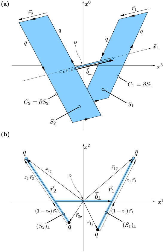
Figure 1: Space-time (a) and transverse (b) arrangement of the Wegner-Wilson loops.

The QCD vacuum expectation value $\langle\ldots\rangle_{G}$ in the loop-loop correlation function (2.3) represents functional integrals [13] in which the functional integration over the fermion fields has already been carried out as indicated by the subscript $G$. The model we use for the QCD vacuum (see Sec. 2.2) describes only gluon dynamics and, thus, implies the quenched approximation that does not allow string breaking through dynamical quark-antiquark production.

2.1 The Loop-Loop Correlation Function

To compute the loop-loop correlation function (2.3), we transform the line integrals over the loops $C_{1,2}$ into integrals over surfaces $S_{1,2}$ with $\partial S_{1,2}=C_{1,2}$ by applying the non-Abelian Stokes’ theorem [28, 13]

$$\Big{\langle}W[C_{1}]W[C_{2}]\Big{\rangle}_{G}=\Big{\langle}\frac{1}{N_{c}}\mbox{Tr}\,{\cal P}_{S}\exp\left[-i\frac{g}{2}\int_{S_{1}}\!d\sigma^{\mu\nu}(x_{1}){\cal G}^{a}_{\mu\nu}(o_{1},x_{1};C_{x_{1}o_{1}})\,t^{a}\right]$$

$$\hphantom{\langle W[C_{1}]W[C_{2}]\rangle_{G}=}\times\frac{1}{N_{c}}\mbox{Tr}\,{\cal P}_{S}\exp\left[-i\frac{g}{2}\int_{S_{2}}\!d\sigma^{\rho\sigma}(x_{2}){\cal G}^{b}_{\rho\sigma}(o_{2},x_{2};C_{x_{2}o_{2}})\,t^{b}\right]\Big{\rangle}_{G}\ ,$$ (2.6)

where the gluon field strength tensors, ${\cal G}_{\mu\nu}(x)={\cal G}_{\mu\nu}^{a}(x)t^{a}$, are parallel transported to the point $o$ along the path $C_{xo}$

$${\cal G}_{\mu\nu}(o,x;C_{xo})=\Phi(x,o;C_{xo})^{-1}{\cal G}_{\mu\nu}(x)\Phi(x,o;C_{xo})$$ (2.7)

with the QCD Schwinger string

$$\Phi(x,o;C_{xo})={\cal P}\exp\left[-ig\int_{C_{xo}}dz^{\mu}{\cal G}_{\mu}(z)\right]\ .$$ (2.8)

In (2.6), ${\cal P}_{S}$ indicates surface ordering and $o_{1}$ and $o_{2}$ are the reference points on the surfaces $S_{1}$ and $S_{2}$, respectively, that enter through the non-Abelian Stokes’ theorem. In order to ensure gauge invariance in our model, the gluon field strengths associated with the loops must be compared at one reference point $o$. Therefore, we require the surfaces $S_{1}$ and $S_{2}$ to touch at a common reference point $o_{1}=o_{2}=o$.

Following the approach of Berger and Nachtmann [14], the product of the two traces (Tr) over $N_{c}\times N_{c}$ matrices in (2.6) is expressed as one trace ($\mbox{Tr}_{2}$) that acts in the $N_{c}^{2}$-dimensional tensor product space of two fundamental $SU(N_{c})$ representations

$$\Big{\langle}W[C_{1}]W[C_{2}]\Big{\rangle}_{G} \!\!\!=\!\!\! \Big{\langle}\frac{1}{N_{c}^{2}}\mbox{Tr}_{2}\left\{\Big{[}\,\,{\cal P}_{S}\exp\big{[}-i\frac{g}{2}\int_{S_{1}}\!d\sigma^{\mu\nu}(x_{1}){\cal G}^{a}_{\mu\nu}(o,x_{1};C_{x_{1}o})\,t^{a}\big{]}\,\,\otimes\,\,{1\!\rm l}\,\,\Big{]}\right.$$ (2.9)

$$\!\!\!\!\times\!\!\!\! \!\!\left.\Big{[}\,\,{1\!\rm l}\,\,\otimes\,\,{\cal P}_{S}\exp\big{[}-i\frac{g}{2}\int_{S_{2}}\!d\sigma^{\rho\sigma}(x_{2}){\cal G}^{b}_{\rho\sigma}(o,x_{2};C_{x_{2}o})\,t^{b}\big{]}\,\,\Big{]}\right\}\Big{\rangle}_{G}.$$

Using the identities

$$\exp\left(\,t^{a}\,\right)\,\otimes\,{1\!\rm l} = \exp\left(\,t^{a}\,\otimes\,{1\!\rm l}\,\right),$$ (2.10)

$${1\!\rm l}\,\otimes\,\exp\left(\,t^{a}\,\right) = \exp\left(\,{1\!\rm l}\,\otimes\,t^{a}\,\right),$$ (2.11)

the tensor products can be shifted into the exponents. With the matrix multiplication in the tensor product space

$$\big{(}t^{a}\,\otimes\,{1\!\rm l}\big{)}\big{(}t^{b}\,\otimes\,{1\!\rm l}\big{)} = t^{a}t^{b}\,\otimes\,{1\!\rm l}\ ,$$

$$\big{(}t^{a}\,\otimes\,{1\!\rm l}\big{)}\big{(}{1\!\rm l}\,\otimes\,t^{b}\big{)} = t^{a}\,\otimes\,t^{b}\ ,$$ (2.12)

and the vanishing commutator

$$\left[t^{a}\otimes{1\!\rm l},{1\!\rm l}\otimes t^{b}\right]=0\ ,$$ (2.13)

the two exponentials in (2.9) commute and can be written as one exponential

$$\Big{\langle}W[C_{1}]W[C_{2}]\Big{\rangle}_{G}=\Big{\langle}\frac{1}{N_{c}^{2}}\mbox{Tr}_{2}\,{\cal P}_{S}\exp\!\left[-i\frac{g}{2}\int_{S}\!d\sigma^{\mu\nu}(x)\hat{\cal{G}}_{\mu\nu}(o,x;C_{xo})\right]\Big{\rangle}_{G}$$ (2.14)

with the following gluon field strength tensor acting in the $N_{c}^{2}$-dimensional tensor product space

$$\hat{\cal{G}}_{\mu\nu}(o,x;C_{xo}):=\left\{\begin{array}[]{cc}{\cal G}_{\mu\nu}^{a}(o,x;C_{xo})\big{(}t^{a}\,\otimes\,{1\!\rm l}\big{)}&\mbox{for $\,\,\,x\,\,\,\in\,\,\,S_{1}$}\\ {\cal G}_{\mu\nu}^{a}(o,x;C_{xo})\big{(}{1\!\rm l}\,\otimes\,t^{b}\big{)}&\mbox{for $\,\,\,x\,\,\,\in\,\,\,S_{2}$}\end{array}\right.\ .$$ (2.15)

In (2.14), the surface integrals over $S_{1}$ and $S_{2}$ are written as one integral over the combined surface $S=S_{1}+S_{2}$. For the evaluation of (2.14), the linearity of the functional integral, $\langle\mbox{Tr}\cdots\rangle=\mbox{Tr}\langle\cdots\rangle$, and a matrix cumulant expansion is used as explained in [13] (cf. also [29])

$$\Big{\langle}{\cal P}_{S}\,\exp\left[-i\frac{g}{2}\int_{S}\!d\sigma(x)\hat{\cal{G}}(o,x;C_{xo})\right]\Big{\rangle}_{G}$$

$$=\exp[\,\,\sum_{n=1}^{\infty}\frac{1}{n!}(-i\frac{g}{2})^{n}\int d\sigma(x_{1})\cdots d\sigma(x_{n})\,K_{n}(x_{1},\cdots,x_{n})]\ ,$$ (2.16)

where Lorentz indices are suppressed to lighten notation. The cumulants $K_{n}$ consist of expectation values of ordered products of the non-commuting matrices $\hat{\cal{G}}(o,z;C_{zo})$. The leading matrix cumulants are

$$K_{1}(x) = \langle\hat{\cal{G}}(o,x;C_{x})\rangle_{G},$$ (2.17)

$$K_{2}(x_{1},x_{2}) = \langle{\cal P}_{S}\,\hat{\cal{G}}(o,x_{1};C_{x_{1}})\hat{\cal{G}}(o,x_{2};C_{x_{2}})\rangle_{G}$$ (2.18)

$$-\frac{1}{2}\left(\langle\hat{\cal{G}}(o,x_{1};C_{x_{1}})\rangle_{G}\langle\hat{\cal{G}}(o,x_{2};C_{x_{2}})\rangle_{G}+(1\leftrightarrow 2)\,\right)\ .$$

Since the vacuum does not prefer a specific color direction, $K_{1}$ vanishes and $K_{2}$ becomes

$$K_{2}(x_{1},x_{2})=\langle{\cal P}_{S}\,\hat{\cal{G}}(o,x_{1};C_{x_{1}})\hat{\cal{G}}(o,x_{2};C_{x_{2}})\rangle_{G}\ .$$ (2.19)

Now, we restrict the functional integral associated with the expectation values $\langle\ldots\rangle_{G}$ to be a Gaussian functional integral. Consequently, all higher cumulants, $K_{n}$ with $n>2$, vanish and the loop-loop correlation function can be expressed in terms of $K_{2}$

$$\!\!\!\!\!\!\!\!\!\!\!\Big{\langle}W[C_{1}]W[C_{2}]\Big{\rangle}_{G}$$

$$\!\!\!\!\!\!\!\!\!\!\!=\frac{1}{N_{c}^{2}}\mbox{Tr}_{2}\exp\!\left[-\frac{g^{2}}{8}\!\int_{S}\!d\sigma^{\mu\nu}(x_{1})\!\int_{S}\!d\sigma^{\rho\sigma}(x_{2})\Big{\langle}{\cal P}_{S}\,\hat{\cal{G}}_{\mu\nu}(o,x_{1};C_{x_{1}o})\hat{\cal{G}}_{\rho\sigma}(o,x_{2};C_{x_{2}o})\Big{\rangle}_{G}\right].$$

(2.20)

Using definition (2.15) and the relations (2.12), we now redivide the exponent in (2.20) into integrals of the ordinary parallel transported gluon field strengths over the separate surfaces $S_{1}$ and $S_{2}$

$$\Big{\langle}W[C_{1}]W[C_{2}]\Big{\rangle}_{G}=\frac{1}{N_{c}^{2}}\mbox{Tr}_{2}\exp\Bigg{[}$$

$$-\frac{g^{2}}{8}\int_{S_{1}}\!d\sigma^{\mu\nu}(x_{1})\int_{S_{2}}\!d\sigma^{\rho\sigma}(x_{2})\,{\cal P}_{S}\,\Big{\langle}{\cal G}^{a}_{\mu\nu}(o,x_{1};C_{x_{1}o}){\cal G}^{b}_{\rho\sigma}(o,x_{2};C_{x_{2}o})\Big{\rangle}_{G}\big{(}t^{a}\,\otimes\,t^{b}\big{)}$$

$$-\frac{g^{2}}{8}\int_{S_{2}}\!d\sigma^{\mu\nu}(x_{1})\int_{S_{1}}\!d\sigma^{\rho\sigma}(x_{2})\,{\cal P}_{S}\,\Big{\langle}{\cal G}^{a}_{\mu\nu}(o,x_{1};C_{x_{1}o}){\cal G}^{b}_{\rho\sigma}(o,x_{2};C_{x_{2}o})\Big{\rangle}_{G}\big{(}t^{a}\,\otimes\,t^{b}\big{)}$$

$$-\frac{g^{2}}{8}\int_{S_{1}}\!d\sigma^{\mu\nu}(x_{1})\int_{S_{1}}\!d\sigma^{\rho\sigma}(x_{2})\,{\cal P}_{S}\,\Big{\langle}{\cal G}^{a}_{\mu\nu}(o,x_{1};C_{x_{1}o}){\cal G}^{b}_{\rho\sigma}(o,x_{2};C_{x_{2}o})\Big{\rangle}_{G}\big{(}t^{a}t^{b}\,\otimes\,{1\!\rm l}\big{)}$$

$$\left.-\frac{g^{2}}{8}\int_{S_{2}}\!d\sigma^{\mu\nu}(x_{1})\int_{S_{2}}\!d\sigma^{\rho\sigma}(x_{2})\,{\cal P}_{S}\,\Big{\langle}{\cal G}^{a}_{\mu\nu}(o,x_{1};C_{x_{1}o}){\cal G}^{b}_{\rho\sigma}(o,x_{2};C_{x_{2}o})\Big{\rangle}_{G}\big{(}{1\!\rm l}\,\otimes\,t^{a}t^{b}\big{)}\,\right]\!.$$

(2.21)

Due to the color-neutrality of the vacuum, the gauge-invariant bilocal gluon field strength correlator contains a $\delta$-function in color-space,

$$\Big{\langle}\frac{g^{2}}{4\pi^{2}}\,{\cal G}^{a}_{\mu\nu}(o,x_{1};C_{x_{1}o}){\cal G}^{b}_{\rho\sigma}(o,x_{2};C_{x_{2}o})\Big{\rangle}_{G}=:\frac{1}{4}\delta^{ab}F_{\mu\nu\rho\sigma}(x_{1},x_{2},o;C_{x_{1}o},C_{x_{2}o})\ ,$$ (2.22)

which makes the surface ordering ${\cal P}_{S}$ in (2.21) irrelevant. The quantity $F_{\mu\nu\rho\sigma}$ will be specified below. With ansatz (2.22) and the definition

$$\chi_{S_{i}S_{j}}:=-\,i\frac{\pi^{2}}{4}\int_{S_{i}}\!d\sigma^{\mu\nu}(x_{1})\int_{S_{j}}\!d\sigma^{\rho\sigma}(x_{2})F_{\mu\nu\rho\sigma}(x_{1},x_{2},o;C_{x_{1}o},C_{x_{2}o})\ ,$$ (2.23)

Eq. (2.21) reads

$$\Big{\langle}W[C_{1}]W[C_{2}]\Big{\rangle}_{G} = \frac{1}{N_{c}^{2}}\mbox{Tr}_{2}\exp\!\Bigg{[}-i\,\frac{1}{2}\Big{\{}\,\left(\chi_{S_{1}S_{2}}+\chi_{S_{2}S_{1}}\right)\big{(}t^{a}\,\otimes\,t^{a}\big{)}$$ (2.24)

$$+\,\chi_{S_{1}S_{1}}\big{(}t^{a}t^{a}\,\otimes\,{1\!\rm l}\big{)}+\chi_{S_{2}S_{2}}\big{(}{1\!\rm l}\,\otimes\,t^{a}t^{a}\big{)}\,\Big{\}}\,\Bigg{]}\ .$$

Our ansatz for the tensor structure of $F_{\mu\nu\rho\sigma}$ — see (2.31), (2.32), and (LABEL:Eq_PGE_Ansatz_F) — leads to $\chi_{S_{1}S_{1}}=\chi_{S_{2}S_{2}}=0$ for light-like loops, as explained in Sec. 2.3, and also to $\chi_{S_{1}S_{2}}=\chi_{S_{2}S_{1}}=:\chi$. For the evaluation of the trace of the remaining exponential, we employ the projectors

$$(P_{s})_{(\alpha_{1}\alpha_{2})(\beta_{1}\beta_{2})}=\frac{1}{2}(\delta_{\alpha_{1}\beta_{1}}\delta_{\alpha_{2}\beta_{2}}+\delta_{\alpha_{1}\beta_{2}}\delta_{\alpha_{2}\beta_{1}}),$$ (2.25)

$$(P_{a})_{(\alpha_{1}\alpha_{2})(\beta_{1}\beta_{2})}=\frac{1}{2}(\delta_{\alpha_{1}\beta_{1}}\delta_{\alpha_{2}\beta_{2}}-\delta_{\alpha_{1}\beta_{2}}\delta_{\alpha_{2}\beta_{1}}),$$ (2.26)

that decompose the direct product space of two fundamental $SU(N_{c})$ representations, in short $\mbox{N}_{c}$, into the irreducible representations

$$\mbox{N}_{c}\,\otimes\,\mbox{N}_{c}=(\mbox{N}_{c}+1)\mbox{N}_{c}/2\,\oplus\,\overline{\mbox{N}_{c}(\mbox{N}_{c}-1)/2}\ .$$ (2.27)

With the identity

$$t^{a}\,\otimes\,t^{a}=\frac{N_{c}-1}{2N_{c}}P_{s}-\frac{N_{c}+1}{2N_{c}}P_{a}\ ,$$ (2.28)

and the projector properties

$$P^{2}_{s,a}=P_{s,a}\ ,\quad\mbox{Tr}_{2}\,P_{s}=(N_{c}+1)N_{c}/2\ ,\quad\mbox{and}\quad\mbox{Tr}_{2}\,P_{a}=(N_{c}-1)N_{c}/2\ ,$$ (2.29)

we find for the loop-loop correlation function in the fundamental $SU(N_{c})$ representation

$$\Big{\langle}W[C_{1}]W[C_{2}]\Big{\rangle}_{G}=\frac{N_{c}+1}{2N_{c}}\exp\!\left[-i\frac{N_{c}-1}{2N_{c}}\chi\right]+\frac{N_{c}-1}{2N_{c}}\exp\!\left[i\frac{N_{c}+1}{2N_{c}}\chi\right]\$$ (2.30)

and recover, of course, for $N_{c}=3$ the result from [14].

2.2 Perturbative and Non-Perturbative QCD Components

We decompose the gauge-invariant bilocal gluon field strength correlator (2.22) into a perturbative ($P$) and non-perturbative ($N\!P$) component

$$F_{\mu\nu\rho\sigma}=F_{\mu\nu\rho\sigma}^{N\!P}+F_{\mu\nu\rho\sigma}^{P}\ .$$ (2.31)

Here, $F_{\mu\nu\rho\sigma}^{N\!P}$ gives the low frequency background field contribution modelled by the non-perturbative stochastic vacuum model (SVM) [15] and $F_{\mu\nu\rho\sigma}^{P}$ the additional high frequency contributions described by perturbative gluon exchange. Such a decomposition is supported by lattice QCD computations of the Euclidean field strength correlator [18, 19].

In the SVM, one makes the approximation that the correlator $F_{\mu\nu\rho\sigma}^{N\!P}$ depends only on the difference $z:=x_{1}-x_{2}$ but not on the reference point $o$ and the curves $C_{x_{1}o}$ and $C_{x_{2}o}$ [15]. Then, the most general form of the correlator that respects translational, Lorentz, and parity invariance reads in four-dimensional Minkowski space-time [11, 12]

$$F_{\mu\nu\rho\sigma}^{N\!P}(z) := F_{\mu\nu\rho\sigma}^{N\!P_{(c)}}(z)+F_{\mu\nu\rho\sigma}^{N\!P_{(nc)}}(z)$$ (2.32)

$$= \frac{1}{3(N_{c}^{2}-1)}\,G_{2}\,\Bigl{\{}\kappa\,\left(g_{\mu\rho}g_{\nu\sigma}-g_{\mu\sigma}g_{\nu\rho}\right)\,D(z^{2}/a^{2})$$

$$+\,(1-\kappa)\,\frac{1}{2}\Bigl{[}\frac{\partial}{\partial z_{\nu}}\left(z_{\sigma}g_{\mu\rho}-z_{\rho}g_{\mu\sigma}\right)+\frac{\partial}{\partial z_{\mu}}\left(z_{\rho}g_{\nu\sigma}-z_{\sigma}g_{\nu\rho}\right)\Bigr{]}\,D_{1}(z^{2}/a^{2})\Bigr{\}}$$

$$= \frac{1}{3(N_{c}^{2}-1)}\,G_{2}\int\frac{d^{4}k}{(2\pi)^{4}}\,e^{-ikz}\,\Bigl{\{}\kappa\,\left(g_{\mu\rho}g_{\nu\sigma}-g_{\mu\sigma}g_{\nu\rho}\right)\,\tilde{D}(k^{2})$$

$$-\,(1-\kappa)\,\Bigl{[}k_{\nu}k_{\sigma}g_{\mu\rho}-k_{\nu}k_{\rho}g_{\mu\sigma}+k_{\mu}k_{\rho}g_{\nu\sigma}-k_{\mu}k_{\sigma}g_{\nu\rho}\Bigr{]}\,\tilde{D}_{1}^{\prime}(k^{2})\Bigr{\}}\ .$$

Here, $a$ is the correlation length, $G_{2}:=\langle\frac{g^{2}}{4\pi^{2}}{\cal G}^{a}_{\mu\nu}(0){\cal G}^{a}_{\mu\nu}(0)\rangle$ is the gluon condensate [30], $\kappa$ determines the non-Abelian character of the correlator, $D$ and $D_{1}$ are correlation functions in four dimensional Minkowski space-time, and

$$\tilde{D}_{1}^{\prime}(k^{2}):=\frac{d}{dk^{2}}\int d^{4}zD_{1}(z^{2}/a^{2})\ e^{ikz}\ .$$ (2.33)

In the case of $\kappa\neq 0$, the Euclidean version of $F_{\mu\nu\rho\sigma}^{N\!P_{(c)}}(z)$ in (2.32) leads to confinement and does not fulfill the Bianchi identity. In contrast, the Euclidean version of $F_{\mu\nu\rho\sigma}^{N\!P_{(nc)}}(z)$ fulfills the Bianchi identity but does not lead to confinement [15]. Therefore, we call the tensor structure multiplied by $\kappa$ non-Abelian or confining ($c$) and the one multiplied by $(1-\kappa)$ Abelian or non-confining ($nc$).

The non-perturbative correlator was originally constructed in Euclidean space-time [15]. The transition to Minkowski space-time is performed by the substitution $\delta_{\mu\rho}\rightarrow-g_{\mu\rho}$ and the analytic continuation of the Euclidean correlation functions to real time, $D^{E}\rightarrow D$ and $D_{1}^{E}\rightarrow D_{1}$ [11, 12]. Euclidean correlation functions are accessible together with the Euclidean correlator in lattice QCD [18, 19]. We adopt for our calculations the simple exponential correlation functions specified in four dimensional Euclidean space-time

$$D^{E}(Z^{2}/a^{2})=D^{E}_{1}(Z^{2}/a^{2})=\exp(-|Z|/a)\ ,$$ (2.34)

that are motivated by lattice QCD measurements of the gluon field strength correlator [18, 19]. These correlation functions stay positive for all Euclidean distances $Z$. In earlier applications of the SVM, a different correlation function $D^{E}$ has been used that becomes negative at large distances [12, 21, 22, 23, 24, 14, 25]. Such a negative part is not compatible with a spectral representation of the correlation function [20]. By analytic continuation of (2.34) we obtain the Minkowski correlation functions in (2.32) as shown in Appendix B.

Treating the vacuum fluctuations as a Gaussian random process, the non-perturbative Euclidean correlator leads to the following explicit expression for the QCD string tension [15]

$$\sigma=\frac{\pi^{3}\kappa G_{2}}{36}\int_{0}^{\infty}dZ^{2}D^{E}(Z^{2}/a^{2})=\frac{\pi^{3}\kappa\,G_{2}\,a^{2}}{18}$$ (2.35)

with the exponential correlation function (2.34) used in the final step. The QCD string tension $\sigma$ characterizes the confining quark-antiquark potential and can be computed from first principles within lattice QCD [31]. Thus, relation (2.35) puts an important constraint on the three fundamental parameters of the non-perturbative QCD vacuum — $a$, $G_{2}$, and $\kappa$ — and eliminates one degree of freedom.

While a non-perturbative model must be used to describe the low frequency contributions, the perturbative component $F_{\mu\nu\rho\sigma}^{P}$ is computed from the gluon propagator in Feynman-’t Hooft gauge

$$\Big{\langle}{\cal G}^{a}_{\mu}(x_{1}){\cal G}^{b}_{\nu}(x_{2})\Big{\rangle}=\int\frac{d^{4}k}{(2\pi)^{4}}\,\frac{-i\delta^{ab}g_{\mu\nu}}{k^{2}-m_{G}^{2}}\,e^{-ik(x_{1}-x_{2})}\ ,$$ (2.36)

with an effective gluon mass $m_{G}$ introduced to limit the range of the perturbative interaction in the infrared (IR) region.

In leading order in the strong coupling $g$, the bilocal gluon field strength correlator is gauge-invariant already without the parallel transport to a common reference point so that $F_{\mu\nu\rho\sigma}^{P}$ depends only on the difference $z:=x_{1}-x_{2}$. In this order, ${\cal O}(g^{2})$, we obtain

$$F_{\mu\nu\rho\sigma}^{P}(z)\!\! = \!\!\frac{g^{2}}{\pi^{2}}\,\frac{1}{2}\Bigl{[}\frac{\partial}{\partial z_{\nu}}\left(z_{\sigma}g_{\mu\rho}-z_{\rho}g_{\mu\sigma}\right)+\frac{\partial}{\partial z_{\mu}}\left(z_{\rho}g_{\nu\sigma}-z_{\sigma}g_{\nu\rho}\right)\Bigr{]}\,D_{P}(z^{2})$$

$$= \!\!-\,\frac{g^{2}}{\pi^{2}}\!\int\!\!\frac{d^{4}k}{(2\pi)^{4}}\,e^{-ikz}\,\Bigl{[}k_{\nu}k_{\sigma}g_{\mu\rho}-k_{\nu}k_{\rho}g_{\mu\sigma}+k_{\mu}k_{\rho}g_{\nu\sigma}-k_{\mu}k_{\sigma}g_{\nu\rho}\Bigr{]}\,\tilde{D}_{P}^{\prime}(k^{2})$$

with the perturbative correlation function

$$\tilde{D}_{P}^{\prime}(k^{2}):=\frac{d}{dk^{2}}\int d^{4}z\,D_{P}(z^{2})\,e^{ikz}=\frac{i}{k^{2}-m_{G}^{2}}\ .$$ (2.38)

The tensor structure in (LABEL:Eq_PGE_Ansatz_F) is identical to the non-confining tensor structure in the non-perturbative component (2.32). Together with the perturbative correlation function in Euclidean space-time, it leads to the non-confining color-Coulomb potential that is dominant for small quark-antiquark separations [32].

In the final step of the computation of $\chi$ in the next section, the constant coupling $g^{2}$ is replaced by the running coupling

$$g^{2}(\vec{z}_{\!\perp})=4\pi\alpha_{s}(\vec{z}_{\!\perp})=\frac{12\pi}{(33-2N_{f})\ln\left[(|\vec{z}_{\!\perp}|^{-2}+M^{2})/\Lambda_{QCD}^{2}\right]}$$ (2.39)

with the renormalization scale provided by $|\vec{z}_{\!\perp}|$ that represents the spatial separation of the interacting dipoles in transverse space. In (2.39), $N_{f}$ denotes the number of dynamical quark flavors, which is set to $N_{f}=0$ in agreement with the quenched approximation, $\Lambda_{QCD}=0.25\;\mbox{GeV}$, and $M^{2}$ allows us to freeze $g^{2}$ for $|\vec{z}_{\!\perp}|\rightarrow\infty$. Relying on a low energy theorem [33], we freeze $g^{2}$ at the value at which the results for the potential and the total flux tube energy of a static quark-antiquark pair coincide in our model [16].

2.3 Evaluation of the $\chi$-Function with Minimal Surfaces

For the computation of the $\chi$-function (2.23)

$$\chi := \chi^{N\!P}_{c}+\chi^{N\!P}_{nc}+\chi^{P}$$ (2.40)

$$= -\,i\,\frac{\pi^{2}}{4}\!\int_{S_{1}}\!d\sigma^{\mu\nu}(x_{1})\int_{S_{2}}\!d\sigma^{\rho\sigma}(x_{2})\left(F_{\mu\nu\rho\sigma}^{N\!P_{(c)}}+F_{\mu\nu\rho\sigma}^{N\!P_{(nc)}}+F_{\mu\nu\rho\sigma}^{P}\right)\ ,$$

one has to specify surfaces $S_{1,2}$ with the restriction $\partial S_{1,2}=C_{1,2}$ according to the non-Abelian Stokes’ theorem. As illustrated in Fig. 1, we put the reference point $o$ at the origin of the coordinate system and choose for $S_{1,2}$ the minimal surfaces that are built from the areas spanned by the corresponding loops $C_{1,2}$ and the infinitesimally thin tube which connects the two surfaces $S_{1}$ and $S_{2}$. Since the tube contributions cancel mutually, this choice makes the calculation explicitly independent of the reference point $o$ and of the paths $C_{x_{1}o}$ and $C_{x_{2}o}$.

The minimal surfaces $S_{1}$ and $S_{2}$ shown in Fig. 1 can be parametrized with the upper (lower) subscripts and signs referring to $S_{1}$ ($S_{2}$) as follows

$$S_{\!\!{1\atop(2)}}=\left\{\Big{(}x^{\mu}_{\!\!\!\!{1\atop(2)}}(u,v)\Big{)}=\Big{(}r^{\mu}_{\!\!\!\!{1q\atop(2q)}}+u\,n^{\mu}_{\!\!\!{\oplus\atop(\ominus)}}+v\,r^{\mu}_{\!\!\!{1\atop(2)}}\Big{)},\;u\in[-T,T],\;v\in[0,1]\right\}\ ,$$ (2.41)

where

$$\Big{(}n^{\mu}_{\!\!\!{\oplus\atop(\ominus)}}\Big{)}:=\left(\begin{array}[]{c}1\\ \vec{0}\\ {\scriptscriptstyle{+\atop(-)}}\!1\end{array}\right),\quad\Big{(}r^{\mu}_{\!\!\!\!{1q\atop(2q)}}\Big{)}:=\left(\begin{array}[]{c}0\\ \vec{r}_{\!\!\!{1q\atop(2q)}}\\ 0\end{array}\right),\quad\mbox{and}\quad\Big{(}r^{\mu}_{\!\!\!{1\atop(2)}}\Big{)}:=\left(\begin{array}[]{c}0\\ \vec{r}_{\!\!\!{1\atop(2)}}\\ 0\end{array}\right)\ .$$ (2.42)

The infinitesimally thin tube is neglected since it does not contribute to the $\chi$-function as already mentioned. The computation of the $\chi$-function requires only the parametrized parts of the minimal surfaces (2.41), the corresponding infinitesimal surface elements

$$d\sigma^{\mu\nu}=\left(\frac{\partial x^{\mu}}{\partial u}\frac{\partial x^{\nu}}{\partial v}-\frac{\partial x^{\mu}}{\partial v}\frac{\partial x^{\nu}}{\partial u}\right)\,du\,dv=\left(n^{\mu}_{\!\!\!{\oplus\atop(\ominus)}}r^{\nu}_{\!\!\!{1\atop(2)}}-r^{\mu}_{\!\!\!{1\atop(2)}}n^{\nu}_{\!\!\!{\oplus\atop(\ominus)}}\right)\,du\,dv\ ,$$ (2.43)

and the limit $T\to\infty$ which is appropriate since the correlation length $a$ is much smaller (see Sec. 2.5) than the longitudinal extension of the loops.

Starting with the confining component

$$\!\!\!\!\!\chi_{c}^{N\!P}:=-\,i\,\frac{\pi^{2}}{4}\int_{S_{1}}\!\!d\sigma^{\mu\nu}(x_{1})\int_{S_{2}}\!\!d\sigma^{\rho\sigma}(x_{2})\,F_{\mu\nu\rho\sigma}^{N\!P_{(c)}}(z=x_{1}-x_{2})$$

$$=-\,\frac{\pi^{2}G_{2}\kappa}{12(N_{c}^{2}-1)}\int_{S_{1}}\!\!d\sigma^{\mu\nu}(x_{1})\int_{S_{2}}\!\!d\sigma^{\rho\sigma}(x_{2})\left(g_{\mu\rho}g_{\nu\sigma}-g_{\mu\sigma}g_{\nu\rho}\right)iD(z^{2}/a^{2})\ ,$$ (2.44)

one exploits the anti-symmetry of the surface elements, $d\sigma^{\mu\nu}=-d\sigma^{\nu\mu}$, and applies the surface parametrization (2.41) with the corresponding surface elements (2.43) to obtain

$$\chi_{c}^{N\!P}=\frac{\pi^{2}G_{2}\kappa}{3(N_{c}^{2}-1)}\,2\left(\vec{r}_{1}\cdot\vec{r}_{2}\right)\int_{0}^{1}\!\!dv_{1}\int_{0}^{1}\!\!dv_{2}\lim_{T\to\infty}\int_{-T}^{T}\!\!du_{1}\int_{-T}^{T}\!\!du_{2}\,iD(z^{2}/a^{2})\ ,$$ (2.45)

where

$$z^{\mu}=x_{1}^{\mu}-x_{2}^{\mu}=u_{1}n^{\mu}_{\oplus}-u_{2}n^{\mu}_{\ominus}+r^{\mu}_{1q}-r^{\mu}_{2q}+v_{1}r^{\mu}_{1}-v_{2}r^{\mu}_{2}\ ,$$ (2.46)

and the identities $n_{\oplus}\cdot r_{2}=r_{1}\cdot n_{\ominus}=0$ and $n_{\oplus}\cdot n_{\ominus}=2$, evident from (2.42), have been used. Next, one Fourier transforms the correlation function and performs the $u_{1}$ and $u_{2}$ integrations in the limit $T\to\infty$

$$\lim_{T\to\infty}\int_{-T}^{T}\!\!du_{1}\int_{-T}^{T}\!\!du_{2}\,iD(z^{2}/a^{2})$$

$$=\int\frac{d^{4}k}{(2\pi)^{4}}\,i\tilde{D}(k^{2})\lim_{T\to\infty}\int_{-T}^{T}\!\!du_{1}\int_{-T}^{T}\!\!du_{2}\,e^{-ikz}$$

$$=\int\frac{d^{4}k}{(2\pi)^{2}}\,i\tilde{D}(k^{2})\,\exp[-ik_{\mu}(r^{\mu}_{1q}-r^{\mu}_{2q}+v_{1}r^{\mu}_{1}-v_{2}r^{\mu}_{2})]\,\delta(k^{0}-k^{3})\,\delta(k^{0}+k^{3})$$

$$=\frac{1}{2}\,iD^{(2)}\left(\vec{r}_{1q}+v_{1}\vec{r}_{1}-\vec{r}_{2q}-v_{2}\vec{r}_{2}\right)\ ,$$ (2.47)

where $iD^{(2)}$ is the confining correlation function in the two-dimensional transverse space (cf. Appendix B)

$$D^{(2)}(\vec{z}_{\!\perp})=\int\frac{d^{2}k_{\!\perp}}{(2\pi)^{2}}e^{i\vec{k}_{\!\perp}\vec{z}_{\!\perp}}\tilde{D}^{(2)}(\vec{k}_{\!\perp})\ .$$ (2.48)

The contributions along the light-cone coordinates have been integrated out so that $\chi_{c}^{N\!P}$ is completely determined by the transverse projection of the minimal surfaces. Inserting (2.47) into (2.45), one finally obtains

$$\chi_{c}^{N\!P}=\frac{\pi^{2}G_{2}}{3(N_{c}^{2}-1)}\,\kappa\left(\vec{r}_{1}\cdot\vec{r}_{2}\right)\,\int_{0}^{1}\!dv_{1}\int_{0}^{1}\!dv_{2}\,iD^{(2)}\left(\vec{r}_{1q}+v_{1}\vec{r}_{1}-\vec{r}_{2q}-v_{2}\vec{r}_{2}\right)\ .$$ (2.49)

With $\tilde{D}^{(2)}(\vec{k}_{\!\perp})$ obtained from the exponential correlation function (2.34), cf. Appendix B, we find

$$iD^{(2)}(\vec{z}_{\!\perp})=2\pi\,a^{2}\left[1+(|\vec{z}_{\!\perp}|/a)\right]\exp\!\left(-|\vec{z}_{\!\perp}|/a\right)$$ (2.50)

which is positive for all transverse distances.

As evident from the $v_{1}$ and $v_{2}$ integrations in (2.49) and Fig. 1b, there are contributions from the transverse projections of the minimal surfaces $(S_{1,2})_{\!\perp}$ connecting the quark and antiquark in each of the two dipoles. We interpret these contributions as a manifestation of the strings that confine the quarks and antiquarks in the dipoles and understand, therefore, the confining component $\chi_{c}^{N\!P}$ as a string-string interaction. This component gives the main contribution to the scattering amplitude in the non-perturbative region [17].

Due to the truncation of the cumulant expansion or, equivalently, the Gaussian approximation, a considerable dependence of $\chi_{c}^{N\!P}$ on the specific surface choice is observed. In fact, a different and more complicated result for $\chi_{c}^{N\!P}$ was obtained with the pyramid mantle choice for the surfaces $S_{1,2}$ in earlier applications of the SVM to high-energy scattering [12, 21, 22, 23, 24, 14, 25]. However, we use minimal surfaces in line with model applications in Euclidean space-time: If one considers the potential of a static quark-antiquark pair, usually the minimal surface is used to obtain Wilson’s area law [15, 16]. Moreover, the simplicity of the minimal surfaces allows us to give an analytic expression for the leading term of the non-perturbative dipole-dipole cross section [17]. Phenomenologically, in comparison with pyramid mantles, the description of the slope parameter $B(s)$, the differential elastic cross section $d\sigma^{el}/dt(s,t)$, and the elastic cross section $\sigma^{el}(s)$ can be improved with minimal surfaces as shown in Sec. 5.

Continuing with the computation of the non-confining component

$$\chi_{nc}^{N\!P}\!\!\!\!\!\! :=-\,i\,\frac{\pi^{2}}{4}\int_{S_{1}}\!\!d\sigma^{\mu\nu}(x_{1})\int_{S_{2}}\!\!d\sigma^{\rho\sigma}(x_{2})\,F_{\mu\nu\rho\sigma}^{N\!P_{(nc)}}(z=x_{1}-x_{2})$$

$$=\frac{\pi^{2}G_{2}(1-\kappa)}{12(N_{c}^{2}-1)}\,\int_{S_{1}}\!\!d\sigma^{\mu\nu}(x_{1})\,\int_{S_{2}}\!\!d\sigma^{\rho\sigma}(x_{2})$$

$$\hphantom{=}\times\int\!\!\frac{d^{4}k}{(2\pi)^{4}}\,e^{-ikz}\,\Bigl{[}k_{\nu}k_{\sigma}g_{\mu\rho}-k_{\nu}k_{\rho}g_{\mu\sigma}+k_{\mu}k_{\rho}g_{\nu\sigma}-k_{\mu}k_{\sigma}g_{\nu\rho}\Bigr{]}\,i\tilde{D}_{1}^{\prime}(k^{2})\ ,$$

we exploit again the anti-symmetry of both surface elements to obtain

$$\chi_{nc}^{N\!P} = \frac{\pi^{2}G_{2}(1-\kappa)}{3(N_{c}^{2}-1)}\,\int_{0}^{1}\!\!dv_{1}\int_{0}^{1}\!\!dv_{2}\,\int\!\!\frac{d^{4}k}{(2\pi)^{4}}\,\lim_{T\to\infty}\,\int_{-T}^{T}\!\!du_{1}\int_{-T}^{T}\!\!du_{2}\,e^{-ikz}$$ (2.52)

$$\times\Bigl{[}2\,(r_{1}\cdot k)\,(r_{2}\cdot k)\,-\,(\vec{r}_{1}\cdot\vec{r}_{2})\,(k^{0}-k^{3})(k^{0}+k^{3})\Bigr{]}\,i\tilde{D}_{1}^{\prime}(k^{2})$$

with $z$ as given in (2.46). Again the identities $n_{\oplus}\cdot r_{2}=r_{1}\cdot n_{\ominus}=0$ and $n_{\oplus}\cdot n_{\ominus}=2$ have been used. Performing the $u_{1}$ and $u_{2}$ integrations in the limit $T\rightarrow\infty$, one obtains — as in (2.47) — two $\delta$-functions which allow us to carry out the integrations over $k^{0}$ and $k^{3}$ immediately. This leads to

$$\chi_{nc}^{N\!P} \!\!\!\!=\!\!\! \frac{\pi^{2}G_{2}(1-\kappa)}{3(N_{c}^{2}-1)}\!\int_{0}^{1}\!\!dv_{1}\!\int_{0}^{1}\!\!dv_{2}\!\int\!\!\frac{d^{2}k_{\!\perp}}{(2\pi)^{2}}i\tilde{D}_{1}^{\prime\,(2)}(\vec{k}_{\!\perp}^{2})(\vec{r}_{1}\cdot\vec{k}_{\!\perp})\,(\vec{r}_{2}\cdot\vec{k}_{\!\perp})e^{i\vec{k}_{\!\perp}(\vec{r}_{1q}+v_{1}\vec{r}_{1}-\vec{r}_{2q}-v_{2}\vec{r}_{2})}$$ (2.53)

$$\!\!\!\!=\!\!\! \frac{\pi^{2}G_{2}(1-\kappa)}{3(N_{c}^{2}-1)}\int_{0}^{1}\!\!dv_{1}\frac{\partial}{\partial v_{1}}\int_{0}^{1}\!\!dv_{2}\frac{\partial}{\partial v_{2}}\,iD_{1}^{\prime\,(2)}(\vec{r}_{1q}+v_{1}\vec{r}_{1}-\vec{r}_{2q}-v_{2}\vec{r}_{2})\ ,$$

where $iD_{1}^{\prime\,(2)}$ is the non-confining correlation function in transverse space defined analogously to (2.48). The $v_{1}$ and $v_{2}$ integrations are trivial and lead (cf. Fig. 1b) to

$$\!\!\!\!\!\!\!\!\!\chi_{nc}^{N\!P}=\frac{\pi^{2}G_{2}}{3(N_{c}^{2}-1)}\,(1-\kappa)\left[iD^{\prime\,(2)}_{1}\left(\vec{r}_{1q}-\vec{r}_{2q}\right)+iD^{\prime\,(2)}_{1}\left(\vec{r}_{1{\bar{q}}}-\vec{r}_{2{\bar{q}}}\right)\right.$$

$$\!\!\!\!\!\!\!\!\!\hphantom{\chi_{nc}^{N\!P}=\frac{\pi^{2}G_{2}}{3(N_{c}^{2}-1)}\,(1-\kappa)}\left.-\,iD^{\prime\,(2)}_{1}\left(\vec{r}_{1q}-\vec{r}_{2{\bar{q}}}\right)-iD^{\prime\,(2)}_{1}\left(\vec{r}_{1{\bar{q}}}-\vec{r}_{2q}\right)\right]\ .$$ (2.54)

Using $\tilde{D}_{1}^{\prime\,(2)}(\vec{k}_{\!\perp}^{2})$, derived from the exponential correlation function (2.34) in Appendix B, we obtain

$$iD^{\prime\,(2)}_{1}(\vec{z}_{\!\perp})=\pi\,a^{4}\left[3+3(|\vec{z}_{\!\perp}|/a)+(|\vec{z}_{\!\perp}|/a)^{2}\right]\exp\!\left(-|\vec{z}_{\!\perp}|/a\right)\ .$$ (2.55)

The non-perturbative components, $\chi^{N\!P}_{c}$ and $\chi^{N\!P}_{nc}$, lead to color transparency for small dipoles, i.e. a dipole-dipole cross section with $\sigma_{DD}(\vec{r}_{1},\vec{r}_{2})\propto|\vec{r}_{1}|^{2}|\vec{r}_{2}|^{2}$ for $|\vec{r}_{1,2}|\to 0$, as known for the perturbative case [34]. This can be seen by squaring (2.49) and (2.54) to obtain the leading terms in the $T$-matrix element for small dipoles (see (2.63)).

The perturbative component $\chi^{P}$ is defined as

$$\chi^{P} := -\,i\,\frac{\pi^{2}}{4}\int_{S_{1}}\!\!d\sigma^{\mu\nu}(x_{1})\int_{S_{2}}\!\!d\sigma^{\rho\sigma}(x_{2})\,F_{\mu\nu\rho\sigma}^{P}(z=x_{1}-x_{2})\hphantom{i\tilde{D}_{P}^{\prime\,(4)}k}$$

$$= \,\frac{g^{2}}{4}\int_{S_{1}}\!\!d\sigma^{\mu\nu}(x_{1})\,\int_{S_{2}}\!\!d\sigma^{\rho\sigma}(x_{2})$$

$$\times\int\!\!\frac{d^{4}k}{(2\pi)^{4}}\,e^{-ikz}\,\Bigl{[}k_{\nu}k_{\sigma}g_{\mu\rho}-k_{\nu}k_{\rho}g_{\mu\sigma}+k_{\mu}k_{\rho}g_{\nu\sigma}-k_{\mu}k_{\sigma}g_{\nu\rho}\Bigr{]}\,i\tilde{D}_{P}^{\prime}(k^{2})\ ,$$

and shows a structure identical to the one of $\chi_{nc}^{N\!P}$ given in (2.3). Accounting for the different prefactors and the different correlation function, the result for $\chi_{nc}^{N\!P}$ (2.54) can be used to obtain

$$\!\!\!\!\!\!\!\!\!\chi^{P}=\left[g^{2}\!\left(\vec{r}_{1q}-\vec{r}_{2q}\right)iD^{\prime\,(2)}_{P}\left(\vec{r}_{1q}-\vec{r}_{2q}\right)+g^{2}\!\left(\vec{r}_{1{\bar{q}}}-\vec{r}_{2{\bar{q}}}\right)iD^{\prime\,(2)}_{P}\left(\vec{r}_{1{\bar{q}}}-\vec{r}_{2{\bar{q}}}\right)\right.$$

$$\!\!\!\!\!\!\!\!\!\!\!\!\!\!\!\!\!\!\!\!\!\hphantom{\chi^{P}=}\left.-\,g^{2}\!\left(\vec{r}_{1q}-\vec{r}_{2{\bar{q}}}\right)iD^{\prime\,(2)}_{P}\left(\vec{r}_{1q}-\vec{r}_{2{\bar{q}}}\right)-g^{2}\!\left(\vec{r}_{1{\bar{q}}}-\vec{r}_{2q}\right)iD^{\prime\,(2)}_{P}\left(\vec{r}_{1{\bar{q}}}-\vec{r}_{2q}\right)\right]\ ,$$ (2.57)

where the running coupling $g^{2}(\vec{z}_{\!\perp})$ is understood as given in (2.39). With (2.38) one obtains the perturbative correlation function in transverse space

$$iD^{\prime\,(2)}_{P}(\vec{z}_{\!\perp})=\frac{1}{2\pi}K_{0}\left(m_{G}|\vec{z}_{\!\perp}|\right)\ ,$$ (2.58)

where $K_{0}$ denotes the $0^{th}$ modified Bessel function (McDonald function).

In contrast to the confining component $\chi_{c}^{N\!P}$, the non-confining components, $\chi_{nc}^{N\!P}$ and $\chi^{P}$, depend only on the transverse position between the quark and antiquark of the two dipoles and are therefore independent of the surface choice.

Finally, we explain that the vanishing of $\chi_{S_{1}S_{1}}$ and $\chi_{S_{2}S_{2}}$ anticipated in Sec. 2.1 results from the light-like loops and the tensor structures in $F_{\mu\nu\rho\sigma}$. Concentrating — without loss of generality — on $\chi_{S_{1}S_{1}}$, the appropriate infinitesimal surface elements (2.43) and the $F_{\mu\nu\rho\sigma}$–ansatz given in (2.31), (2.32), and (LABEL:Eq_PGE_Ansatz_F) are inserted into (2.23). Having simplified the resulting expression by exploiting the anti-symmetry of the surface elements, one finds only terms proportional to $n_{\oplus}^{2}$, $n_{\oplus}\cdot r_{1}$, and $n_{\oplus}\cdot z$ with $z^{\mu}=x_{1}^{\mu}-x_{2}^{\mu}=(u_{1}-u_{2})n^{\mu}_{\oplus}+(v_{1}-v_{2})r^{\mu}_{1}$. Since $n_{\oplus}^{2}=0$ and $n_{\oplus}\cdot r_{1}=0$, which is evident from (2.42), all terms vanish and $\chi_{S_{1}S_{1}}=0$ is derived.

Note that $\chi=\chi_{c}^{N\!P}+\chi_{nc}^{N\!P}+\chi^{P}$ is a real-valued function. Since, in addition, the wave functions $|\psi_{i}(z_{i},\vec{r}_{i})|^{2}$ used in this work (cf. Appendix A) are invariant under the replacement $(\vec{r}_{i}\rightarrow-\vec{r}_{i},z_{i}\rightarrow 1-z_{i})$, the $T$-matrix element becomes purely imaginary and reads for $N_{c}=3$

$$\!\!\!\!\!\!\!\!\!\!\!\!\!T(s,t) = 2is\int\!\!d^{2}b_{\!\perp}e^{i{\vec{q}}_{\!\perp}{\vec{b}}_{\!\perp}}\int\!\!dz_{1}d^{2}r_{1}\!\int\!\!dz_{2}d^{2}r_{2}\,\,|\psi_{1}(z_{1},\vec{r}_{1})|^{2}\,\,|\psi_{2}(z_{2},\vec{r}_{2})|^{2}$$ (2.59)

$$\!\!\!\!\!\!\!\!\!\!\times\left[1-\frac{2}{3}\cos\!\left(\frac{1}{3}\chi({\vec{b}}_{\!\perp},z_{1},\vec{r}_{1},z_{2},\vec{r}_{2})\!\right)-\frac{1}{3}\cos\!\left(\frac{2}{3}\chi({\vec{b}}_{\!\perp},z_{1},\vec{r}_{1},z_{2},\vec{r}_{2})\!\right)\right].$$

The real part averages out in the integration over ${\vec{r}}_{i}$ and $z_{i}$ since the $\chi$-function changes sign

$$\chi(\vec{b}_{\!\perp},1-z_{1},-\vec{r}_{1},z_{2},\vec{r}_{2})=-\chi(\vec{b}_{\!\perp},z_{1},\vec{r}_{1},z_{2},\vec{r}_{2})\ ,$$ (2.60)

which can be seen directly from (2.49),(2.54) and (2.57) as $(\vec{r}_{1}\rightarrow-\vec{r}_{1},z_{1}\rightarrow 1-z_{1})$ implies $\vec{r}_{1q}\rightarrow\vec{r}_{1{\bar{q}}}$. In physical terms, $(\vec{r}_{i}\rightarrow-\vec{r}_{i},z_{i}\rightarrow 1-z_{i})$ corresponds to charge conjugation  i.e. the replacement of each parton with its antiparton and the associated reversal of the loop direction.

Consequently, the $T$-matrix (2.59) describes only charge conjugation $C=+1$ exchange. Since in our quenched approximation purely gluonic interactions are modelled, (2.59) describes only pomeron but not reggeon exchange.

2.4 Energy Dependence

Until now, the derived $T$-matrix element leads to energy independent total cross sections in contradiction to the experimental observation. In this section, we introduce the energy dependence in a phenomenological way inspired by other successful models.

Most models for high-energy scattering are constructed to describe either hadron-hadron or photon-hadron reactions. For example, Kopeliovich et al. [35] as well as Berger and Nachtmann [14] focus on hadron-hadron scattering. In contrast, Golec-Biernat and Wüsthoff [9] and Forshaw, Kerley, and Shaw [36] concentrate on photon-proton reactions. A model that describes the energy dependence in both hadron-hadron and photon-hadron reactions up to large photon virtualities is the two-pomeron model of Donnachie and Landshoff [6]. Based on Regge theory, they find a soft pomeron trajectory with intercept $1+\epsilon_{soft}\approx 1.08$ that governs the weak energy dependence of hadron-hadron or $\gamma^{*}p$ reactions with low $Q^{2}$ and a hard pomeron trajectory with intercept $1+\epsilon_{hard}\approx 1.4$ that governs the strong energy dependence of $\gamma^{*}p$ reactions with high $Q^{2}$. Similarly, we aim at a simultaneous description of hadron-hadron, photon-proton, and photon-photon reactions involving real and virtual photons as well.

In line with other two-component (soft $+$ hard) models [6, 24, 36, 23, 37] and the different hadronization mechanisms in soft and hard collisions, our physical ansatz demands that the perturbative and non-perturbative contributions do not interfere. Therefore, we modify the cosine-summation in (2.59) allowing only even numbers of soft and hard correlations, $\left(\chi^{N\!P}\right)^{2n}\left(\chi^{P}\right)^{2m}$ with $n,m\in I\!\!N$. Interference terms with odd numbers of soft and hard correlations are subtracted by the replacement

$$\cos\left[c\chi\right]=\cos\left[c\left(\chi^{N\!P}+\chi^{P}\right)\right]\rightarrow\cos\left[c\chi^{N\!P}\right]\cos\left[c\chi^{P}\right]\ ,$$ (2.61)

where $c=1/3$ or $2/3$. This prescription leads to the following factorization of soft and hard physics in the $T$-matrix element,

$$\!\!\!\!\!\!\!\!\!\!T(s,t)=2is\int\!\!d^{2}b_{\!\perp}e^{i{\vec{q}}_{\!\perp}{\vec{b}}_{\!\perp}}\int\!\!dz_{1}d^{2}r_{1}\!\int\!\!dz_{2}d^{2}r_{2}\,\,|\psi_{1}(z_{1},\vec{r}_{1})|^{2}\,\,|\psi_{2}(z_{2},\vec{r}_{2})|^{2}$$

$$\!\!\!\!\!\!\!\!\!\!\!\!\times\left[1-\frac{2}{3}\cos\!\left(\!\frac{1}{3}\chi^{N\!P}\!\right)\cos\!\left(\!\frac{1}{3}\chi^{P}\!\right)-\frac{1}{3}\cos\!\left(\!\frac{2}{3}\chi^{N\!P}\!\right)\cos\!\left(\!\frac{2}{3}\chi^{P}\!\right)\right]\ .$$ (2.62)

In the limit of small $\chi$-functions, $\chi^{N\!P}\ll 1$ and $\chi^{P}\ll 1$, one gets

$$T(s,t) = 2is\!\int\!\!d^{2}b_{\!\perp}e^{i{\vec{q}}_{\!\perp}{\vec{b}}_{\!\perp}}\!\int\!\!dz_{1}d^{2}r_{1}\!\int\!\!dz_{2}d^{2}r_{2}\,\,|\psi_{1}(z_{1},\vec{r}_{1})|^{2}\,\,|\psi_{2}(z_{2},\vec{r}_{2})|^{2}$$ (2.63)

$$\times\frac{1}{9}\left[\left(\chi^{N\!P}\right)^{2}+\left(\chi^{P}\right)^{2}\right].$$

In this limit, the $T$-matrix element evidently becomes a sum of a perturbative and a non-perturbative component. Of course, the perturbative component, $(\chi^{P})^{2}$, coincides with the well-known perturbative two-gluon exchange [17]. Correspondingly, the non-perturbative component, $(\chi^{N\!P})^{2}$, represents the non-perturbative gluonic interaction on the “two-gluon-exchange” level.

As the two-component structure of (2.63) reminds of the two-pomeron model of Donnachie and Landshoff [6], we adopt the powerlike energy increase and ascribe a weak energy dependence to the non-perturbative component $\chi^{N\!P}$ and a strong one to the perturbative component $\chi^{P}$

$$\left(\chi^{N\!P}\right)^{2}\quad \rightarrow \quad\left(\chi^{N\!P}(s)\right)^{2}:=\left(\chi^{N\!P}\right)^{2}\left(\frac{s}{s_{0}}\frac{\vec{r}_{1}^{\,2}\,\vec{r}_{2}^{\,2}}{R_{0}^{4}}\right)^{\epsilon^{N\!P}}$$

$$\left(\chi^{P}\right)^{2}\quad \rightarrow \quad\left(\chi^{P}(s)\right)^{2}:=\left(\chi^{P}\right)^{2}\left(\frac{s}{s_{0}}\frac{\vec{r}_{1}^{\,2}\,\vec{r}_{2}^{\,2}}{R_{0}^{4}}\right)^{\epsilon^{P}}$$ (2.64)

with the scaling factor $s_{0}R_{0}^{4}$. The powerlike energy dependence with the exponents $0\approx\epsilon^{N\!P}<\epsilon^{P}<1$ guarantees Regge type behavior at moderately high energies, where the small-$\chi$ limit (2.63) is appropriate. In (2.64), the energy variable $s$ is scaled by the factor $\vec{r}_{1}^{\,2}\,\vec{r}_{2}^{\,2}$ that allows to rewrite the energy dependence in photon-hadron scattering in terms of the appropriate Bjorken scaling variable $x$

$$s\,\vec{r}_{1}^{\,2}\propto\frac{s}{Q^{2}}=\frac{1}{x}\ ,$$ (2.65)

where $|\vec{r}_{1}|$ is the transverse extension of the $q{\bar{q}}$ dipole in the photon. A similar factor has been used before in the dipole model of Forshaw, Kerley, and Shaw [36] and also in the model of Donnachie and Dosch [37] in order to respect the scaling properties observed in the structure function of the proton. In the dipole-proton cross section of Golec-Biernat and Wüsthoff [9], Bjorken $x$ is used directly as energy variable which is important for the success of the model. In fact, also in our model, the $\vec{r}_{1}^{\,2}\,\vec{r}_{2}^{\,2}$ factor improves the description of $\gamma^{*}p$ reactions at large $Q^{2}$.

The powerlike Regge type energy dependence introduced in (2.64) is, of course, not mandatory but allows successful fits and can also be derived in other theoretical frameworks: A powerlike energy dependence is found for hadronic reactions by Kopeliovich et al. [35] and for hard photon-proton reactions from the BFKL equation [8]. However, these approaches need unitarization since their powerlike energy dependence will ultimately violate $S$-matrix unitarity at asymptotic energies. In our model, we use the following $T$-matrix element as the basis for the rest of this work

$$\!\!\!\!\!\!\!\!\!\!T(s,t)=2is\int\!\!d^{2}b_{\!\perp}e^{i{\vec{q}}_{\!\perp}{\vec{b}}_{\!\perp}}\int\!\!dz_{1}d^{2}r_{1}\!\int\!\!dz_{2}d^{2}r_{2}\,\,|\psi_{1}(z_{1},\vec{r}_{1})|^{2}\,\,|\psi_{2}(z_{2},\vec{r}_{2})|^{2}$$

$$\!\!\!\!\!\!\!\!\!\!\!\!\times\left[1-\frac{2}{3}\cos\!\left(\!\frac{1}{3}\chi^{N\!P}(s)\!\right)\cos\!\left(\!\frac{1}{3}\chi^{P}(s)\!\right)-\frac{1}{3}\cos\!\left(\!\frac{2}{3}\chi^{N\!P}(s)\!\right)\cos\!\left(\!\frac{2}{3}\chi^{P}(s)\!\right)\right]\ ,$$

(2.66)

where the cosine functions ensure the unitarity condition in impact parameter space as shown in Sec. 3. Indeed, the multiple gluonic interactions associated with the higher order terms in the expansion of the cosine functions are important for the saturation effects observed within our model at ultra-high energies.

Having ascribed the energy dependence to the $\chi$-function, the energy behavior of hadron-hadron, photon-hadron, and photon-photon scattering results exclusively from the universal loop-loop correlation function $S_{DD}$.

2.5 Model Parameters

Lattice QCD simulations provide important information and constraints on the model parameters. The fine tuning of the parameters was, however, directly performed on the high-energy scattering data for hadron-hadron, photon-hadron, and photon-photon reactions where an error ($\chi^{2}$) minimization was not feasible because of the non-trivial multi-dimensional integrals in the $T$-matrix element (2.66).

The parameters $a$, $\kappa$, $G_{2}$, $m_{G}$, $M^{2}$, $s_{0}R^{4}_{0}$, $\epsilon^{N\!P}$ and $\epsilon^{P}$ determine the dipole-dipole scattering and are universal for all reactions described. In addition, there are reaction-dependent parameters associated with the wave functions which are provided in Appendix A.

The non-perturbative component involves the correlation length $a$, the gluon condensate $G_{2}$, and the parameter $\kappa$ indicating the non-Abelian character of the correlator. With the simple exponential correlation functions specified in Euclidean space-time (2.34), we obtain the following values for the parameters of the non-perturbative correlator (2.32)

$$a=0.302\,\mbox{fm},\quad\kappa=0.74,\quad G_{2}=0.074\,\mbox{GeV}^{4}\ ,$$ (2.67)

and, correspondingly, the string tension

$$\sigma=\frac{\pi^{3}\kappa\,G_{2}\,a^{2}}{18}=0.22\,\mbox{GeV}^{2}\equiv 1.12\,\mbox{GeV}/\mbox{fm}\ ,$$ (2.68)

which is consistent with hadron spectroscopy [38], Regge theory [39], and lattice QCD investigations [31].

Lattice QCD computations of the gluon field strength correlator down to distances of $0.4\,\mbox{fm}$ have obtained the following values with the exponential correlation function (2.34) [19]: $a=0.219\,\mbox{fm}$, $\kappa=0.746$, $G_{2}=0.173\,\mbox{GeV}^{4}$. This value for $\kappa$ is in agreement with the one in (2.67), while the fit to high-energy scattering data clearly requires a larger value for $a$ and a smaller value for $G_{2}$.

The perturbative component involves the gluon mass $m_{G}$ as IR regulator (or inverse “perturbative correlation length”) and the parameter $M^{2}$ that freezes the running coupling (2.39) for large distance scales at the value $\alpha_{s}=0.4$, where the non-perturbative component of our model with the above ingredients is at work according to a low energy theorem [33, 16]. We adopt the parameters

$$m_{G}=m_{\rho}=0.77\,\mbox{GeV}\quad\mbox{and }\quad M^{2}=1.04\,\mbox{GeV}^{2}\ .$$ (2.69)

The energy dependence of the model is associated with the energy exponents $\epsilon^{N\!P}$ and $\epsilon^{P}$, and the scaling parameter $s_{0}R^{4}_{0}$

$$\epsilon^{N\!P}=0.125,\quad\epsilon^{P}=0.73,\quad\mbox{and}\quad s_{0}R_{0}^{4}=(\,47\,\mbox{GeV}\,\mbox{fm}^{2}\,)^{2}\ .$$ (2.70)

In comparison with the energy exponents of Donnachie and Landshoff [7, 6], $\epsilon_{soft}\approx 0.08$ and $\epsilon_{hard}\approx 0.4$, our exponents are larger. However, the cosine functions in our $T$-matrix element (2.66) reduce the large exponents so that the energy dependence of the cross sections agrees with the experimental data as illustrated in Sec 5.

3 Impact Parameter Profiles and $S$-Matrix Unitarity

In this section, the $S$-matrix unitarity is analysed in our model. On the basis of the impact parameter dependence of the scattering amplitude, saturation effects can be exposed that manifest the unitarity of the $S$-matrix. For each impact parameter the energy at which the unitarity limit becomes important can be determined. This is used to show the saturation of the gluon distribution and to localize saturation effects in experimental observables.

The impact parameter dependence of the scattering amplitude is given by ${\cal T}(s,|\vec{b}_{\!\perp}|)$,

$$T(s,t=-{\vec{q}}_{\!\perp}^{\,\,2})\;=\;4s\!\int\!\!d^{2}b_{\!\perp}\,e^{i{\vec{q}}_{\!\perp}{\vec{b}}_{\!\perp}}\,{\cal T}(s,|\vec{b}_{\!\perp}|)$$ (3.1)

and in particular by the profile function

$$J(s,|\vec{b}_{\!\perp}|)=2\,\mbox{Im}{\cal T}(s,|\vec{b}_{\!\perp}|)\ ,$$ (3.2)

which describes the blackness or opacity of the interacting particles as a function of the impact parameter $|{\vec{b}}_{\!\perp}|$ and the c.m. energy $\sqrt{s}$. In fact, the profile function (3.2) determines every observable if the $T$-matrix is — as in our model — purely imaginary.

The $S$-matrix unitarity, $SS^{\dagger}=S^{\dagger}S={1\!\rm l}$, leads directly to the unitarity condition in impact parameter space [40, 41]

$$\mbox{Im}{\cal T}(s,|\vec{b}_{\!\perp}|)=|{\cal T}(s,|\vec{b}_{\!\perp}|)|^{2}+G_{inel}(s,|\vec{b}_{\!\perp}|)\ ,$$ (3.3)

where $G_{inel}(s,|\vec{b}_{\!\perp}|)\geq 0$ is the inelastic overlap function [42]. This unitarity condition imposes an absolute limit on the profile function

$$0\;\;\leq\;\;2\,|{\cal T}(s,|\vec{b}_{\!\perp}|)|^{2}\;\;\leq\;\;J(s,|\vec{b}_{\!\perp}|)\;\;\leq\;\;2$$ (3.4)

and the inelastic overlap function, $G_{inel}(s,|\vec{b}_{\!\perp}|)\leq 1/4$. At high energies, however, the elastic amplitude is expected to be purely imaginary. Consequently, the solution of (3.3) reads

$$J(s,|\vec{b}_{\!\perp}|)=1\pm\sqrt{1-4\,G_{inel}(s,|\vec{b}_{\!\perp}|)}$$ (3.5)

and leads with the minus sign corresponding to the physical situation to the reduced unitarity bound

$$0\;\;\leq\;\;J(s,|\vec{b}_{\!\perp}|)\;\;\leq\;\;1\ .$$ (3.6)

Reaching the black disc limit or maximum opacity at a certain impact parameter $|\vec{b}_{\!\perp}|$, $J(s,|\vec{b}_{\!\perp}|)=1$, corresponds to maximal inelastic absorption $G_{inel}(s,|\vec{b}_{\!\perp}|)=1/4$ and equal elastic and inelastic contributions to the total cross section at that impact parameter.

In our model, every reaction is reduced to dipole-dipole scattering with well defined dipole sizes $|{\vec{r}}_{i}|$ and longitudinal quark momentum fractions $z_{i}$. The unitarity condition in our model becomes, therefore, most explicit in the profile function

$$J_{DD}(s,|\vec{b}_{\!\perp}|,z_{1},|\vec{r}_{1}|,z_{2},|\vec{r}_{2}|)=\int\frac{d\phi_{1}}{2\pi}\int\frac{d\phi_{2}}{2\pi}\left[1-S_{DD}(s,\vec{b}_{\!\perp},z_{1},{\vec{r}}_{1},z_{2},{\vec{r}}_{2})\right]\ ,$$ (3.7)

where $\phi_{i}$ describes the dipole orientation, i.e. the angle between ${\vec{r}}_{i}$ and $\vec{b}_{\!\perp}$, and $S_{DD}$ describes elastic dipole-dipole scattering

$$S_{DD}=\frac{2}{3}\cos\!\left(\frac{1}{3}\chi^{N\!P}(s)\right)\cos\!\left(\frac{1}{3}\chi^{P}(s)\right)+\frac{1}{3}\cos\!\left(\frac{2}{3}\chi^{N\!P}(s)\right)\cos\!\left(\frac{2}{3}\chi^{P}(s)\right)$$ (3.8)

with the purely real-valued eikonal functions $\chi^{N\!P}(s)$ and $\chi^{P}(s)$ defined in (2.64). Because of $|S_{DD}|\leq 1$, a consequence of the cosine functions in (3.8) describing multiple gluonic interactions, $J_{DD}$ respects the absolute limit (3.4). Thus, the elastic dipole-dipole scattering respects the unitarity condition (3.3). At high energies, the arguments of the cosine functions in $S_{DD}$ become so large that these cosines average to zero in the integration over the dipole orientations. This leads to the black disc limit $J_{DD}^{max}=1$ reached at high energies first for small impact parameters.

If one considers the scattering of two dipoles with fixed orientation, the inelastic overlap function obtained from the unitarity constraint (3.3),

$$\!\!\!\!\!\!\!\!G_{inel}^{DD}(s,|\vec{b}_{\!\perp}|)$$ (3.9)

$$\!\!\!\!\!\!\!\!=\frac{1}{4}\left(1-\left[\frac{2}{3}\cos\!\left(\frac{1}{3}\chi^{N\!P}(s)\right)\cos\!\left(\frac{1}{3}\chi^{P}(s)\right)+\frac{1}{3}\cos\!\left(\frac{2}{3}\chi^{N\!P}(s)\right)\cos\!\left(\frac{2}{3}\chi^{P}(s)\right)\right]^{2}\right)\ ,$$

shows nonphysical behavior with increasing energy. This behavior is a consequence of aritifically fixing the orientations of the dipoles. If one averages over the dipole orientations as in all high-energy reactions considered in this work, no unphysical behavior is observed.

3.1 The Profile Function for Proton-Proton Scattering

The profile function for proton-proton scattering

$$J_{pp}(s,|\vec{b}_{\!\perp}|)=\int\!\!dz_{1}d^{2}r_{1}\!\int\!\!dz_{2}d^{2}r_{2}|\psi_{p}(z_{1},\vec{r}_{1})|^{2}|\psi_{p}(z_{2},\vec{r}_{2})|^{2}\left[1-S_{DD}(s,\vec{b}_{\!\perp},z_{1},{\vec{r}}_{1},z_{2},{\vec{r}}_{2})\right]$$ (3.10)

is obtained from (3.7) by weighting the dipole sizes $|{\vec{r}}_{i}|$ and longitudinal quark momentum fractions $z_{i}$ with the proton wave function $|\psi_{p}(z_{i},\vec{r}_{i})|^{2}$ from Appendix A.

Using the model parameters from Sec. 2.5, one obtains the profile function $J_{pp}(s,|\vec{b}_{\!\perp}|)$ shown in Fig. 2 for c.m. energies from $\sqrt{s}=10\,\mbox{GeV}$ to $\sqrt{s}=10^{8}\,\mbox{GeV}$.

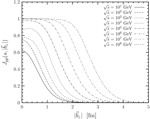
Figure 2: The profile function for proton-proton scattering $J_{pp}(s,|\vec{b}_{\!\perp}|)$ is shown versus the impact parameter $|\vec{b}_{\!\perp}|$ for c.m. energies from $\sqrt{s}=10\,\mbox{GeV}$ to $\sqrt{s}=10^{8}\,\mbox{GeV}$. The unitarity limit (3.4) corresponds to $J_{pp}(s,|\vec{b}_{\!\perp}|)=2$ and the black disc limit (3.6) to $J_{pp}(s,|\vec{b}_{\!\perp}|)=1$.

Up to $\sqrt{s}\approx 100\,\mbox{GeV}$, the profile has approximately a Gaussian shape. Above $\sqrt{s}=1\,\mbox{TeV}$, it significantly develops into a broader and higher profile until the black disc limit is reached for $\sqrt{s}\approx 10^{6}\,\mbox{GeV}$ and $|\vec{b}_{\!\perp}|=0$. At this point, the cosine functions in $S_{DD}$ average to zero

$$\int\!\!dz_{1}d^{2}r_{1}\!\int\!\!dz_{2}d^{2}r_{2}|\psi_{p}(z_{1},{\vec{r}}_{1})|^{2}|\psi_{p}(z_{2},{\vec{r}}_{2})|^{2}S_{DD}(\sqrt{s}\gtrsim 10^{6}\,\mbox{GeV},|\vec{b}_{\!\perp}|=0,\dots)\approx 0$$ (3.11)

so that the proton wave function normalization determines the maximum opacity

$$J_{pp}^{max}=\int\!\!dz_{1}d^{2}r_{1}\!\int\!\!dz_{2}d^{2}r_{2}\,|\psi_{p}(z_{1},{\vec{r}}_{1})|^{2}\,|\psi_{p}(z_{2},{\vec{r}}_{2})|^{2}=1\ .$$ (3.12)

Once the maximum opacity is reached at a certain impact parameter, the profile function saturates at that $|\vec{b}_{\!\perp}|$ and extends towards larger impact parameters with increasing energy. Thus, the multiple gluonic interactions important to respect the $S$-matrix unitarity constraint (3.3) lead to saturation for $\sqrt{s}\gtrsim 10^{6}\,\mbox{GeV}$.

The above behavior of the profile function illustrates the evolution of the proton with increasing c.m. energy. The proton is gray and of small transverse size at small $\sqrt{s}$ but becomes blacker and more transversally extended with increasing $\sqrt{s}$ until it reaches the black disc limit in its center at $\sqrt{s}\approx 10^{6}\,\mbox{GeV}$. Beyond this energy, the proton cannot become blacker in its central region but in its periphery with continuing transverse growth. Furthermore, the proton boundary seems to stay diffusive as claimed also in [43].

According to our model the black disc limit will not be reached at LHC. Our prediction of $\sqrt{s}\approx 10^{6}\,\mbox{GeV}=10^{3}\,\mbox{TeV}$ for the onset of the black disc limit in proton-proton collisions is about two orders of magnitude beyond the LHC energy $\sqrt{s}=14\,\mbox{TeV}$. This is in contrast, for example, with [44], where the value predicted for the onset of the black disc limit is $\sqrt{s}=2\,\mbox{TeV}$, i.e. small enough to be reached at LHC. However, we feel confidence in our LHC prediction since our profile function $J_{pp}(s,|\vec{b}_{\!\perp}|)$ yields good agreement with experimental data for cross sections up to the highest energies as shown in Sec. 5.

For hadron-hadron reactions in general, the wave function normalization of the hadrons determines the maximum opacity analogous to (3.12) and the transverse hadron size the c.m. energy at which it is reached. Consequently, the maximum opacity obtained for $\pi p$ and $Kp$ scattering is identical to the one for $pp$ scattering due to the normalization (A.2). Furthermore, the smaller size of pions and kaons in comparison to protons demands slightly higher c.m. energies to reach this maximum opacity. This size effect becomes more apparent in longitudinal photon-proton scattering, where the size of the dipole emerging from the photon can be controlled by the photon virtuality.

3.2 The Profile Function for Photon-Proton Scattering

The profile function for a longitudinal photon $\gamma_{L}^{*}$ scattering off a proton $p$

$$J_{\gamma_{L}^{*}p}(s,|\vec{b}_{\!\perp}|,Q^{2}) = \int\!\!dz_{1}d^{2}r_{1}\!\int\!\!dz_{2}d^{2}r_{2}\,|\psi_{\gamma_{L}^{*}}(z_{1},\vec{r}_{1},Q^{2})|^{2}\,|\psi_{p}(z_{2},\vec{r}_{2})|^{2}$$ (3.13)

$$\times\left[1-S_{DD}(\vec{b}_{\!\perp},s,z_{1},{\vec{r}}_{1},z_{2},{\vec{r}}_{2})\right]$$

is calculated with the longitudinal photon wave function $|\psi_{\gamma_{L}^{*}}(z_{i},\vec{r}_{i},Q^{2})|^{2}$ given in (A.5). In this way, the profile function (3.13) is ideally suited for the investigation of dipole size effects since the photon virtuality $Q^{2}$ determines the transverse size of the dipole into which the photon fluctuates before it interacts with the proton.

Figure 3 shows the $|\vec{b}_{\!\perp}|$ dependence of the profile function $J_{\gamma_{L}^{*}p}(s,|\vec{b}_{\!\perp}|,Q^{2})$ divided by $\alpha/{\pi}$ for c.m. energies $\sqrt{s}$ from $10\,\mbox{GeV}$ to $10^{9}\,\mbox{GeV}$ and a photon virtuality of $Q^{2}=1\,\mbox{GeV}^{2}$, where $\alpha$ is the fine-structure constant.

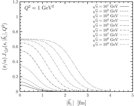
Figure 3: The profile function for a longitudinal photon scattering off a proton $J_{\gamma_{L}^{*}p}(s,|\vec{b}_{\!\perp}|,Q^{2})$ divided by $\alpha/{\pi}$ is shown versus the impact parameter $|\vec{b}_{\!\perp}|$ at a photon virtuality of $Q^{2}=1\,\mbox{GeV}^{2}$ and c.m. energies from $\sqrt{s}=10\,\mbox{GeV}$ to $\sqrt{s}=10^{9}\,\mbox{GeV}$. The value of the black disc limit is $J_{\gamma_{L}^{*}p}^{max}(Q^{2}=1\,\mbox{GeV}^{2})=0.00164$ .

One clearly sees that the qualitative behavior of this rescaled profile function is similar to the one for proton-proton scattering. However, the black disc limit induced by the underlying dipole-dipole scattering depends on the photon virtuality $Q^{2}$ and is given by the normalization of the longitudinal photon wave function

$$J_{\gamma_{L}^{*}p}^{max}(Q^{2})=\int\!\!dzd^{2}r|\psi_{\gamma_{L}^{*}}(z,\vec{r},Q^{2})|^{2}$$ (3.14)

since the proton wave function is normalized to one.

The photon virtuality $Q^{2}$ does not only determine the absolute value of the black disc limit but also the c.m. energy at which it is reached. This is illustrated in Fig. 4, where the $\sqrt{s}$ dependence of $J_{\gamma_{L}^{*}p}(s,|\vec{b}_{\!\perp}|=0,Q^{2})$ divided by $\alpha/{\pi}$ is presented for $Q^{2}=1,\,10,\,\mbox{and}\,100\,\mbox{GeV}^{2}$.

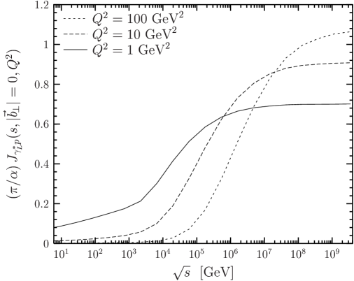
Figure 4: The profile function for a longitudinal photon scattering off a proton $J_{\gamma_{L}^{*}p}(s,|\vec{b}_{\!\perp}|,Q^{2})$ divided by $\alpha/{\pi}$ is shown versus the c.m. energy $\sqrt{s}$ at zero impact parameter ($|\vec{b}_{\!\perp}|=0$) for photon virtualities $Q^{2}=1,\,10,\,\mbox{and}\,100\,\mbox{GeV}^{2}$.

With increasing resolution $Q^{2}$, i.e. decreasing dipole sizes, $|\vec{r}_{\gamma_{L}^{*}}|^{2}\propto 1/Q^{2}$, the absolute value of the black disc limit grows and higher energies are needed to reach this limit. The growth of the absolute value of the black disc limit is simply due to the normalization of the longitudinal photon wave function while the requirement of higher energies to reach this limit is due to the decreasing interaction strength with decreasing dipole size. The latter explains also why the energies needed to reach the black disc limit in $\pi p$ and $Kp$ scattering are higher than in $pp$ scattering. Comparing $\gamma_{L}^{*}p$ scattering at $Q^{2}=1\,\mbox{GeV}^{2}$ with $pp$ scattering quantitatively, the black disc limit $J_{\gamma_{L}^{*}p}^{max}(Q^{2}=1\,\mbox{GeV}^{2})=0.00164$ is about three orders of magnitude smaller because of the photon wave function normalization ($\propto\alpha/{\pi}$). At $|\vec{b}_{\!\perp}|=0$ it is reached at an energy of $\sqrt{s}\approx 10^{8}\,\mbox{GeV}$, which is about two orders of magnitude higher because of the smaller dipoles involved.

The way in which the profile function $J_{\gamma_{L}^{*}p}(s,|\vec{b}_{\!\perp}|,Q^{2})$ approaches the black disc limit at high energies depends on the shape of the proton and longitudinal photon wave function at small dipole sizes $|\vec{r}_{1,2}|$. At high energies, dipoles of typical sizes $0\leq|\vec{r}_{1,2}|\leq R_{0}\,(s_{0}/s)^{1/4}$ give the main contribution to $S_{\gamma_{L}^{*}p}=1-J_{\gamma_{L}^{*}p}$ because of (2.64) and the fact that the contribution of the large dipole sizes averages to zero upon integration over the dipole orientations, cf. also (3.11). Since $S_{\gamma_{L}^{*}p}$ is a measure of the proton transmittance, this means that only small dipoles can penetrate the proton at high energies. Increasing the energy further, even these small dipoles are absorbed and the black disc limit is reached. However, the dependence of the profile function on the short distance behavior of normalizable wave functions is weak which can be understood as follows. Because of color transparency, the eikonal functions $\chi^{N\!P}(s)$ and $\chi^{P}(s)$ are small for small dipole sizes $0\leq|\vec{r}_{1,2}|\leq R_{0}\,(s_{0}/s)^{1/4}$ at large $\sqrt{s}$. Consequently, $S_{DD}\approx 1$ and

$$\!\!\!\!\!\!\!\!\!\!\!\!\!\!\!\!J_{\gamma_{L}^{*}p}(s,|\vec{b}_{\!\perp}|,Q^{2})$$

$$\!\!\!\!\!\!\!\!\!\!\!\!\!\!\!\!\approx J_{\gamma_{L}^{*}p}^{max}(Q^{2})-4\pi^{2}\!\!\int\limits_{0}^{1}\!\!dz_{1}\!\!\int\limits_{0}^{r_{c}(s)}\!\!\!dr_{1}r_{1}|\psi_{\gamma_{L}^{*}}(z_{1},r_{1},Q^{2})|^{2}\int\limits_{0}^{1}\!\!dz_{2}\!\!\int\limits_{0}^{r_{c}(s)}\!\!\!dr_{2}r_{2}|\psi_{p}(z_{2},r_{2})|^{2}$$ (3.15)

where $r_{c}(s)\approx R_{0}\,(s_{0}/s)^{1/4}$. Clearly, the linear behavior from the phase space factors $r_{1,2}$ dominates over the $r_{1,2}$-dependence of normalizable wave functions. More generally, for any profile function involving normalizable wave functions, the way in which the black disc limit is approached depends only weakly on the short distance behavior of the wave functions.

4 A Scenario for Gluon Saturation

In this section, we estimate the impact parameter dependent gluon distribution of the proton $xG(x,Q^{2},|\vec{b}_{\!\perp}|)$. Using a leading twist, next-to-leading order QCD relation between $xG(x,Q^{2})$ and the longitudinal structure function $F_{L}(x,Q^{2})$, we relate $xG(x,Q^{2},|\vec{b}_{\!\perp}|)$ to the profile function $J_{\gamma_{L}^{*}p}(s=Q^{2}/x,|\vec{b}_{\!\perp}|,Q^{2})$ and find low-$x$ saturation of $xG(x,Q^{2},|\vec{b}_{\!\perp}|)$ as a manifestation of $S$-matrix unitarity. The resulting $xG(x,Q^{2},|\vec{b}_{\!\perp}|)$ is, of course, only an estimate since our profile function contains also higher twist contributions. Furthermore, in the considered low-$x$ region, the leading twist, next-to-leading order QCD formula may be inadequate as higher twist contributions [45] and higher order QCD corrections [46, 47] are expected to become important. Nevertheless, still assuming a close relation between $F_{L}(x,Q^{2})$ and $xG(x,Q^{2})$ at low $x$, we think that our approach provides some insight into the gluon distribution as a function of the impact parameter and into its saturation.

The gluon distribution of the proton $~{}xG(x,Q^{2})~{}$ has the following meaning: $xG(x,Q^{2})dx$ gives the momentum fraction of the proton which is carried by the gluons in the interval $[x,x+dx]$ as seen by probes of virtuality $Q^{2}$. The impact parameter dependent gluon distribution $xG(x,Q^{2},|\vec{b}_{\!\perp}|)$ is the gluon distribution $xG(x,Q^{2})$ at a given impact parameter $|\vec{b}_{\!\perp}|$ so that

$$xG(x,Q^{2})=\int\!\!d^{2}b_{\!\perp}\,xG(x,Q^{2},|\vec{b}_{\!\perp}|)\ .$$ (4.1)

In leading twist, next-to-leading order QCD, the gluon distribution $xG(x,Q^{2})$ is related to the structure functions $F_{L}(x,Q^{2})$ and $F_{2}(x,Q^{2})$ of the proton [48]

$$F_{L}(x,Q^{2})=\frac{\alpha_{s}}{\pi}\!\left[\frac{4}{3}\int_{x}^{1}\!\frac{dy}{y}\!\left(\frac{x}{y}\right)^{\!\!2}\!F_{2}(y,Q^{2})+2\sum_{f}e_{f}^{2}\!\int_{x}^{1}\!\frac{dy}{y}\!\left(\frac{x}{y}\right)^{\!\!2}\!\!\left(\!1-\frac{x}{y}\right)yG(y,Q^{2})\right]$$ (4.2)

where $\sum_{f}e_{f}^{2}$ is a flavor sum over the quark charges squared. For four active flavors and $x\lesssim 10^{-3}$, (4.2) can be approximated as follows [49]

$$xG(x,Q^{2})\approx\frac{3}{5}\,5.8\,\left[\frac{3\pi}{4\alpha_{s}}\,F_{L}(0.417x,Q^{2})-\frac{1}{1.97}\,F_{2}(0.75x,Q^{2})\right]\ .$$ (4.3)

For typical $\Lambda_{QCD}=100-300\,\mbox{MeV}$ and $Q^{2}=50-100\,\mbox{GeV}^{2}$, the coefficient of $F_{L}$ in (4.3), $3\pi/(4\alpha_{s})={\cal{O}}(10)$, is large compared to the one of $F_{2}$. Taking into account also the values of $F_{2}$ and $F_{L}$, in this $Q^{2}$ region and for $x\lesssim 10^{-3}$, the gluon distribution is mainly determined by the longitudinal structure function. The latter can be expressed in terms of the profile function for longitudinal photon-proton scattering using the optical theorem (cf. (5.1))

$$F_{L}(x,Q^{2})=\frac{Q^{2}}{4\,\pi^{2}\,\alpha}\,\sigma^{tot}_{\gamma^{*}_{L}p}(x,Q^{2})=\frac{Q^{2}}{4\,\pi^{2}\,\alpha}\,2\!\int\!\!d^{2}b_{\!\perp}\,J_{\gamma_{L}^{*}p}(x,|\vec{b}_{\!\perp}|,Q^{2})\ ,$$ (4.4)

where the $s$-dependence of the profile function is rewritten in terms of the Bjorken scaling variable, $x=Q^{2}/s$. Neglecting the $F_{2}$ term in (4.3), consequently, the gluon distribution reduces to

$$xG(x,Q^{2})\approx 1.305\,\frac{Q^{2}}{\pi^{2}\alpha_{s}}\,\frac{\pi}{\alpha}\int\!\!d^{2}b_{\!\perp}\,J_{\gamma_{L}^{*}p}(0.417x,|\vec{b}_{\!\perp}|,Q^{2})\ .$$ (4.5)

Comparing (4.1) with (4.5), it seems natural to relate the integrand of (4.5) to the impact parameter dependent gluon distribution

$$xG(x,Q^{2},|\vec{b}_{\!\perp}|)\approx 1.305\,\frac{Q^{2}}{\pi^{2}\alpha_{s}}\,\frac{\pi}{\alpha}\,J_{\gamma_{L}^{*}p}(0.417x,|\vec{b}_{\!\perp}|,Q^{2})\ .$$ (4.6)

The black disc limit of the profile function for longitudinal photon-proton scattering (3.14) imposes accordingly an upper bound on $xG(x,Q^{2},|\vec{b}_{\!\perp}|)$

$$xG(x,Q^{2},|\vec{b}_{\!\perp}|)\ \leq\ xG^{max}(Q^{2})\approx 1.305\,\frac{Q^{2}}{\pi^{2}\alpha_{s}}\,\frac{\pi}{\alpha}\,J_{\gamma^{*}_{L}p}^{max}(Q^{2})\ ,$$ (4.7)

which is the low-$x$ saturation value of the gluon distribution $xG(x,Q^{2},|\vec{b}_{\!\perp}|)$ in our approach. With $\pi J_{\gamma^{*}_{L}p}^{max}(Q^{2})/\alpha\approx 1$ as shown in Fig. 4, a compact approximation of (4.7) is obtained

$$xG(x,Q^{2},|\vec{b}_{\!\perp}|)\ \leq\ xG^{max}(Q^{2})\approx\frac{Q^{2}}{\pi^{2}\alpha_{s}}\ ,$$ (4.8)

which is consistent with the results in [47, 50, 51] and indicates strong color-field strengths $G^{a}_{\mu\nu}\sim 1/\sqrt{\alpha_{s}}$ as well.

According to our relations (4.6) and (4.7), the blackness described by the profile function is a measure for the gluon distribution and the black disc limit corresponds to the maximum gluon distribution reached at the impact parameter under consideration. In accordance with the behavior of the profile function $J_{\gamma_{L}^{*}p}$, see Fig. 3, the gluon distribution $xG(x,Q^{2},|\vec{b}_{\!\perp}|)$ decreases with increasing impact parameter for given values of $x$ and $Q^{2}$. The gluon density, consequently, has its maximum in the geometrical center of the proton, i.e. at zero impact parameter, and decreases towards the periphery. With decreasing $x$ at given $Q^{2}$, the gluon distribution $xG(x,Q^{2},|\vec{b}_{\!\perp}|)$ increases and extends towards larger impact parameters just as the profile function $J_{\gamma_{L}^{*}p}$ for increasing $s$. The saturation of the gluon distribution $xG(x,Q^{2},|\vec{b}_{\!\perp}|)$ sets in first in the center of the proton ($|\vec{b}_{\!\perp}|=0$) at very small Bjorken $x$.

In Fig. 5, the gluon distribution $xG(x,Q^{2},|\vec{b}_{\!\perp}|=0)$ is shown as a function of $x$ for $Q^{2}=1,\,10,\,\mbox{and}\,100\,\mbox{GeV}^{2}$, where the relation (4.6) has been used also for low photon virtualities.

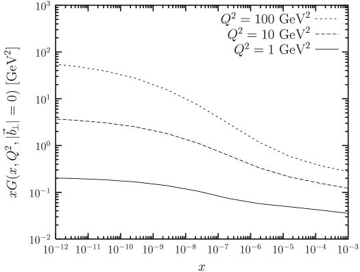
Figure 5: The gluon distribution of the proton at zero impact parameter $xG(x,Q^{2},|\vec{b}_{\!\perp}|=0)$ is shown as a function of $x$ for $Q^{2}=1,\,10,\,\mbox{and}\,100\,\mbox{GeV}^{2}$. The results are obtained within the approximation (4.6).

Evidently, the gluon distribution $xG(x,Q^{2},|\vec{b}_{\!\perp}|=0)$ saturates at very low values of $x\lesssim 10^{-10}$ for $Q^{2}\gtrsim 1\,\mbox{GeV}^{2}$. The photon virtuality $Q^{2}$ determines the saturation value (4.7) and the Bjorken-$x$ at which it is reached (cf. also Fig. 3). For larger $Q^{2}$, the low-$x$ saturation value is larger and is reached at smaller values of $x$, as claimed also in [52]. Moreover, the growth of $xG(x,Q^{2},|\vec{b}_{\!\perp}|=0)$ with decreasing $x$ becomes stronger with increasing $Q^{2}$. This results from the stronger energy increase of the perturbative component, $\epsilon^{P}=0.73$, that becomes more important with decreasing dipole size.

According to our approach, the onset of the $xG(x,Q^{2},|\vec{b}_{\!\perp}|)$-saturation appears for $Q^{2}\gtrsim 1\,\mbox{GeV}^{2}$ at $x\lesssim 10^{-10}$, which is far below the $x$-region accessible at HERA ($x\gtrsim 10^{-6}$). Even for THERA ($x\gtrsim 10^{-7}$), gluon saturation is not predicted for $Q^{2}\gtrsim 1\,\mbox{GeV}^{2}$. However, since the HERA data can be described by models with and without saturation embedded [52], the present situation is not conclusive.

Note that the $S$-matrix unitarity condition (3.3) together with (4.6) requires the saturation of the impact parameter dependent gluon distribution $xG(x,Q^{2},|\vec{b}_{\!\perp}|)$ but not the saturation of the integrated gluon distribution $xG(x,Q^{2})$. Due to multiple gluonic interactions in our model, this requirement is fulfilled, as can be seen from Fig. 3 and relation (4.6). Indeed, approximating the gluon distribution $xG(x,Q^{2},|\vec{b}_{\!\perp}|)$ in the saturation regime of very low $x$ by a step-function

$$xG(x,Q^{2},|\vec{b}_{\!\perp}|)\approx xG^{max}(Q^{2})\,\Theta(\,R(x,Q^{2})-|\vec{b}_{\!\perp}|\,)\ ,$$ (4.9)

where $R(x,Q^{2})$ denotes the full width at half maximum of the profile function, one obtains with (4.1), (4.7) and (4.8) the integrated gluon distribution

$$xG(x,Q^{2})\;\approx\;1.305\,\frac{Q^{2}\,R^{2}(x,Q^{2})}{\pi\alpha_{s}}\,\frac{\pi}{\alpha}\,J_{\gamma^{*}_{L}p}^{max}(Q^{2})\;\approx\;\frac{Q^{2}\,R^{2}(x,Q^{2})}{\pi\alpha_{s}}\ ,$$ (4.10)

which does not saturate because of the increase of the effective proton radius $R(x,Q^{2})$ with decreasing $x$. Nevertheless, although $xG(x,Q^{2})$ does not saturate, the saturation of $xG(x,Q^{2},|\vec{b}_{\!\perp}|)$ leads to a slow-down in its growth towards small $x$. Interestingly, our result (4.10) coincides with the result of Mueller and Qiu [47].

Finally, it must be emphasized that the low-$x$ saturation of $xG(x,Q^{2},|\vec{b}_{\!\perp}|)$, required in our approach by the $S$-matrix unitarity, is realized by multiple gluonic interactions. In other approaches that describe the evolution of the gluon distribution with varying $x$ and $Q^{2}$, gluon recombination leads to gluon saturation [46, 47, 54, 55, 56], which is reached when the probability of a gluon splitting up into two is equal to the probability of two gluons fusing into one. A more phenomenological understanding of saturation is attempted in [9, 57].

5 Comparison with Experimental Data

In this section, we discuss the phenomenological performance of our model. We compute total, differential, and elastic cross sections, structure functions, and diffractive slopes for hadron-hadron, photon-proton, and photon-photon scattering, compare the results with experimental data including cosmic ray data, and provide predictions for future experiments. Having studied the saturation of the impact parameter profiles, we show here how this manifestation of unitarity translates into the quantities mentioned above and how it could become observable.

Using the $T$-matrix (2.66) with the parameters and wave functions from Sec. 2.5 and Appendix A, we compute the pomeron contribution to $pp$, $p{\bar{p}}$, $\pi^{\pm}p$, $K^{\pm}p$, $\gamma^{*}p$, and $\gamma\gamma$ reactions in terms of the universal dipole-dipole scattering amplitude $S_{DD}$. This allows one to compare reactions induced by hadrons and photons in a systematic way. In fact, it is our aim to provide a unified description of all these reactions and to show in this way that the pomeron contribution to the above reactions is universal and can be traced back to the dipole-dipole scattering amplitude $S_{DD}$.

Our model describes pomeron ($C=+1$ gluon exchange) but neither odderon ($C=-1$ gluon exchange) nor reggeon exchange (quark-antiquark exchange) as discussed in Sec. 2.3. Only in the computation of the hadronic total cross sections the reggeon contribution is added [7, 58]. This improves the agreement with the data for $\sqrt{s}\lesssim 100\,\mbox{GeV}$ and describes exactly the differences between $ab$ and $\bar{a}b$ reactions.

The fine tuning of the model and wave function parameters was performed on the data shown below. The resulting parameter set given in Sec. 2.5 and Appendix A is used throughout this paper.

5.1 Total Cross Sections

The total cross section for the high-energy reaction $ab\to X$ is related via the optical theorem to the imaginary part of the forward elastic scattering amplitude and can also be expressed in terms of the profile function (3.2)

$$\sigma^{tot}_{ab}(s)\;=\;\frac{1}{s}\,\mbox{Im}\,T(s,t=0)\;=\;2\int\!d^{2}b_{\!\perp}\,J_{ab}(s,|\vec{b}_{\!\perp}|)\ ,$$ (5.1)

where $a$ and $b$ label the initial particles whose masses were neglected as they are small in comparison to the c.m. energy $\sqrt{s}$.

We compute the pomeron contribution to the total cross section, $\sigma^{tot,I\!\!P}_{ab}(s)$, from the $T$-matrix (2.66), as explained above, and add only here a reggeon contribution of the form [7, 58]

$$\sigma^{tot,I\!\!R}_{ab}(s)=X_{ab}\,\left(\frac{s}{1\,\mbox{GeV}^{2}}\right)^{-0.4525}\ ,$$ (5.2)

where $X_{ab}$ depends on the reaction considered: $X_{pp}=56.08\,\mbox{mb}$, $X_{p{\bar{p}}}=98.39\,\mbox{mb}$, $X_{\pi^{+}p}=27.56\,\mbox{mb}$, $X_{\pi^{-}p}=36.02\,\mbox{mb}$, $X_{K^{+}p}=8.15\,\mbox{mb}$, $X_{K^{-}p}=26.36\,\mbox{mb}$, $X_{\gamma p}=0.129\,\mbox{mb}$, and $X_{\gamma\gamma}=605\,\mbox{nb}$. Accordingly, we obtain the total cross section

$$\sigma^{tot}_{ab}(s)=\sigma^{tot,I\!\!P}_{ab}(s)+\sigma^{tot,I\!\!R}_{ab}(s)$$ (5.3)

for $pp$, $p{\bar{p}}$, $\pi^{\pm}p$, $K^{\pm}p$, $\gamma p$ and $\gamma\gamma$ scattering.

The good agreement of the computed total cross sections with the experimental data is shown in Fig. 6.

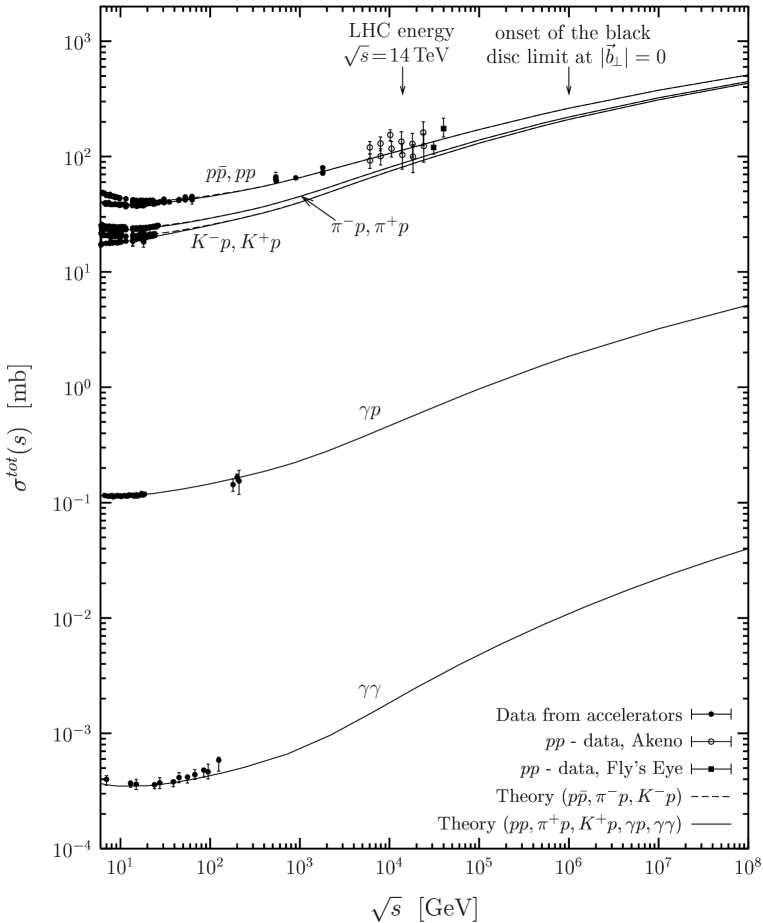
Figure 6: The total cross section $\sigma^{tot}$ is shown as a function of the c.m. energy $\sqrt{s}$ for $pp$, $p{\bar{p}}$, $\pi^{\pm}p$, $K^{\pm}p$, $\gamma p$ and $\gamma\gamma$ scattering. The solid lines represent the model results for $pp$, $\pi^{+}p$, $K^{+}p$, $\gamma p$ and $\gamma\gamma$ scattering and the dashed lines the ones for $p{\bar{p}}$, $\pi^{-}p$, and $K^{-}p$ scattering. The $pp$, $p{\bar{p}}$, $\pi^{\pm}p$, $K^{\pm}p$, $\gamma p$ [1] and $\gamma\gamma$ data [59] taken at accelerators are indicated by the closed circles while the closed squares (Fly’s eye data) [60] and the open circles (Akeno data) [61] indicate cosmic ray data. The arrows at the top point to the LHC energy, $\sqrt{s}=14\,\mbox{TeV}$, and to the onset of the black disc limit in $pp$ ($p{\bar{p}}$) reactions, $\sqrt{s}\approx 10^{6}\,\mbox{GeV}$.

Here, the solid lines represent the theoretical results for $pp$, $\pi^{+}p$, $K^{+}p$, $\gamma p$, and $\gamma\gamma$ scattering and the dashed lines the ones for $p{\bar{p}}$, $\pi^{-}p$, and $K^{-}p$ scattering. The $pp$, $p{\bar{p}}$, $\pi^{\pm}p$, $K^{\pm}p$, $\gamma p$ [1] and $\gamma\gamma$ data [59] taken at accelerators are indicated by the closed circles while the closed squares (Fly’s eye data) [60] and the open circles (Akeno data) [61] indicate cosmic ray data. Concerning the photon-induced reactions, only real photons are considered which are, of course, only transverse polarized.

The prediction for the total $pp$ cross section at LHC ($\sqrt{s}=14\,\mbox{TeV}$) is $\sigma^{tot}_{pp}=114.2\,\mbox{mb}$ in good agreement with the cosmic ray data. Compared with other works, our LHC prediction is close to the one of Block et al. [62], $\sigma^{tot}_{pp}=108\pm 3.4\,\mbox{mb}$, but considerably larger than the one of Donnachie and Landshoff [7], $\sigma^{tot}_{pp}=101.5\,\mbox{mb}$.

The differences between $ab$ and $\bar{a}b$ reactions for $\sqrt{s}\lesssim 100\,\mbox{GeV}$ result solely from the different reggeon contributions which die out rapidly as the energy increases. The pomeron contribution to $ab$ and $\bar{a}b$ reactions is, in contrast, identical and increases as the energy increases. It thus governs the total cross sections for $\sqrt{s}\gtrsim 100\,\mbox{GeV}$ where the results for $ab$ and $\bar{a}b$ reactions coincide.

The differences between $pp$ ($p{\bar{p}}$), $\pi^{\pm}p$, and $K^{\pm}p$ scattering result from the different transverse extension parameters, $S_{p}=0.86\,\mbox{fm}>S_{\pi}=0.607\,\mbox{fm}>S_{K}=0.55\,\mbox{fm}$, cf. Appendix A. Since a smaller transverse extension parameter favors smaller dipoles, the total cross section becomes smaller, and the short distance physics described by the perturbative component becomes more important and leads to a stronger energy growth due to $\epsilon^{P}=0.73>\epsilon^{N\!P}=0.125$. In fact, the ratios $\sigma^{tot}_{pp}/\sigma^{tot}_{\pi p}$ and $\sigma^{tot}_{pp}/\sigma^{tot}_{Kp}$ converge slowly towards unity with increasing energy as can already be seen in Fig. 6.

For real photons, the transverse size is governed by the constituent quark masses $m_{f}(Q^{2}=0)$, cf. Appendix A, where the light quarks have the strongest effect, i.e. $\sigma^{tot}_{\gamma p}\propto 1/m_{u,d}^{2}$ and $\sigma^{tot}_{\gamma\gamma}\propto 1/m_{u,d}^{4}$. Furthermore, in comparison with hadron-hadron scattering, there is the additional suppression factor of $\alpha$ for $\gamma p$ and $\alpha^{2}$ for $\gamma\gamma$ scattering coming from the photon-dipole transition. In the $\gamma\gamma$ reaction, also the box diagram contributes [63, 58] but is neglected since its contribution to the total cross section is less than 1% [37].

It is worthwhile mentioning that total cross sections for $pp$ ($p{\bar{p}}$), $\pi^{\pm}p$, and $K^{\pm}p$ scattering do not depend on the longitudinal quark momentum distribution in the hadrons since the underlying dipole-dipole cross section is independent of the longitudinal quark momentum fraction $z_{i}$ for $t=0$. We show this analytically on the two-gluon-exchange level in [17].

Saturation effects as a manifestation of the $S$-matrix unitarity can be seen in Fig. 6. Having investigated the profile function for $pp$ ($p{\bar{p}}$) scattering, we know that this profile function becomes higher and broader with increasing energy until it saturates the black disc limit first for zero impact parameter ($|\vec{b}_{\!\perp}|=0$) at $\sqrt{s}\approx 10^{6}\,\mbox{GeV}$. Beyond this energy, the profile function cannot become higher but expands towards larger values of $|\vec{b}_{\!\perp}|$. Consequently, the total cross section (5.1) increases no longer due to the growing blackness at the center but only due to the transverse expansion of the hadrons. This tames the growth of the total cross section as can be seen for the total $pp$ cross section beyond $\sqrt{s}\approx 10^{6}\,\mbox{GeV}$ in Fig. 6.

At energies beyond the onset of the black disc limit at zero impact parameter, the profile function can be approximated by

$$J_{ab}^{approx}(s,|\vec{b}_{\!\perp}|)=N_{a}\,N_{b}\,\Theta\left(R(s)-|\vec{b}_{\!\perp}|\right)\,$$ (5.4)

where $N_{a,b}$ denotes the normalization of the wave functions of the scattered particles and $R(s)$ the full width at half maximum of the exact profile function $J_{ab}(s,|\vec{b}_{\!\perp}|)$ that reflects the effective radii of the interacting particles. Thus, the energy dependence of the total cross section (5.1) is driven exclusively by the increase of the transverse extension of the particles $R(s)$

$$\sigma^{tot}_{ab}(s)=2\pi N_{a}N_{b}R(s)^{2}\ ,$$ (5.5)

which is known as geometrical scaling [64, 65]. The growth of $R(s)$ can at most be logarithmic for $\sqrt{s}\to\infty$ because of the Froissart-Lukaszuk-Martin bound [5]. In fact, a transition from a power-like to an $\ln^{2}$-increase of the total $pp$ cross section seems to set in at about $\sqrt{s}\approx 10^{6}\,\mbox{GeV}$ as visible in Fig. 6. Moreover, since the hadronic cross sections join for $\sqrt{s}\to\infty$, $R(s)$ becomes independent of the hadron-hadron reaction considered at asymptotic energies as long as $N_{a,b}=1$. Also for photons of different virtuality $Q_{1}^{2}$ and $Q_{2}^{2}$ one can check that the ratio of the total cross sections $\sigma^{tot}_{\gamma^{*}p}(Q_{1}^{2})/\sigma^{tot}_{\gamma^{*}p}(Q_{2}^{2})$ converges to unity at asymptotic energies in agreement with the conclusion in [66].

5.2 The Proton Structure Function

The total cross section for the scattering of a transverse ($T$) and longitudinally ($L$) polarized photon off the proton, $\sigma_{\gamma^{*}_{T\!,L}p}^{tot}(x,Q^{2})$, at photon virtuality $Q^{2}$ and c.m. energy squared, $s=Q^{2}/x$, is equivalent to the structure functions of the proton

$$F_{T,L}(x,Q^{2})=\frac{Q^{2}}{4\pi^{2}\alpha}\sigma_{\gamma^{*}_{T\!,L}p}^{tot}(x,Q^{2})$$ (5.6)

and

$$F_{2}(x,Q^{2})=F_{T}(x,Q^{2})+F_{L}(x,Q^{2})\ .$$ (5.7)

Reactions induced by virtual photons are particularly interesting because the transverse separation of the quark-antiquark pair that emerges from the virtual photon decreases as the photon virtuality increases (cf. Appendix A)

$$|\vec{r}_{\gamma}|\approx\frac{2}{\sqrt{Q^{2}+4m_{u,d}^{2}}}\ ,$$ (5.8)

where $m_{u,d}$ is a mass of the order of the constituent $u$-quark mass. With increasing virtuality, one probes therefore smaller transverse distance scales of the proton.

In Fig. 7, the $Q^{2}$-dependence of the total $\gamma^{*}p$ cross section

$$\sigma^{tot}_{\gamma^{*}p}(s,Q^{2})=\sigma^{tot}_{\gamma_{T}^{*}p}(s,Q^{2})+\sigma^{tot}_{\gamma_{L}^{*}p}(s,Q^{2})$$ (5.9)

is presented, where the model results (solid lines) are compared with the experimental data for c.m. energies from $\sqrt{s}=20\,\mbox{GeV}$ up to $\sqrt{s}=245\,\mbox{GeV}$. Note the indicated scaling factors at different $\sqrt{s}$ values. The low energy data at $\sqrt{s}=20\,\mbox{GeV}$ are from [67] while the data at higher energies have been measured at HERA by the H1 [68] and ZEUS collaboration [69]. At $Q^{2}=0.012\,\mbox{GeV}^{2}$, also the photoproduction ($Q^{2}=0$) data from [70] are displayed.

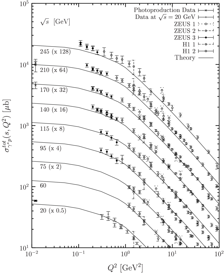
Figure 7: The total $\gamma^{*}p$ cross section, $\sigma^{tot}_{\gamma^{*}p}(s,Q^{2})$, is shown as a function of the photon virtuality $Q^{2}$ for c.m. energies from $\sqrt{s}=20\,\mbox{GeV}$ to $\sqrt{s}=245\,\mbox{GeV}$, where the model results (solid lines) and the experimental data at different $\sqrt{s}$ values are scaled with the indicated factors. The low energy data at $\sqrt{s}=20\,\mbox{GeV}$ are from [67], the data at higher energies from the H1 [68] and ZEUS collaboration [69]. The photoproduction ($Q^{2}=0$) data from [70] are displayed at $Q^{2}=0.012\,\mbox{GeV}^{2}$.

In the window shown in Fig. 7, the model results are in reasonable agreement with the experimental data. The total $\gamma^{*}p$ cross section levels off towards small values of $Q^{2}$ as soon as the photon size $|\vec{r}_{\gamma}|$, i.e the resolution scale, becomes comparable to the proton size. Our model reproduces this behavior by using the perturbative photon wave functions with $Q^{2}$-dependent quark masses, $m_{f}(Q^{2})$, that interpolate between the current (large $Q^{2}$) and the constituent (small $Q^{2}$) quark masses as explained in detail in Appendix A. The decrease of $\sigma^{tot}_{\gamma^{*}p}$ with increasing $Q^{2}$ results from the decreasing dipole sizes since small dipoles do not interact as strongly as large dipoles.

The $x$-dependence of the computed proton structure function $F_{2}(x,Q^{2})$ is shown in Fig. 8 for $Q^{2}=0.3,\,2.5,\,12$ and $120\,\mbox{GeV}^{2}$ in comparison to the data measured by the H1 [71] and ZEUS [72] detector.

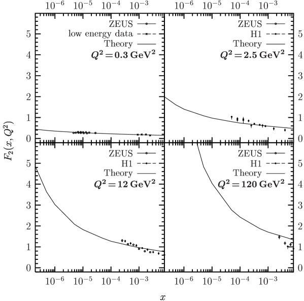
Figure 8: The $x$-dependence of the computed proton structure function $F_{2}(x,Q^{2})$ (solid line) is shown for $Q^{2}=0.3,\,2.5,\,12$ and $120\,\mbox{GeV}^{2}$ in comparison to the data measured by the H1 [71] and ZEUS [72] detector, and the low energy data at $\sqrt{s}=20\,\mbox{GeV}$ from [67].

Within our model, the increase of $F_{2}(x,Q^{2})$ towards small Bjorken $x$ becomes stronger with increasing $Q^{2}$ in agreement with the trend in the HERA data. This behavior results from the fast energy growth of the perturbative component that becomes more important with increasing $Q^{2}$ due to the smaller dipole sizes involved.

As can be seen in Fig. 8, the data show a stronger increase with decreasing $x$ than the model outside the low-$Q^{2}$ region. This results from the weak energy boost of the non-perturbative component that dominates $F_{2}(x,Q^{2})$ in our model. In fact, even for large $Q^{2}$ the non-perturbative contribution overwhelms the perturbative one, which explains also the overestimation of the data for $x\gtrsim 10^{-3}$.

This problem is typical for the SVM model applied to the scattering of a small size dipole off a proton. In an earlier application by Rüter [23], an additional cut-off was introduced to switch from the non-perturbative to the perturbative contribution as soon as one of the dipoles is smaller than $r_{cut}=0.16\,\mbox{fm}$. This yields a better agreement with the data also for large $Q^{2}$ but leads to a discontinuous dipole-proton cross section. In the model of Donnachie and Dosch [37], a similar SVM-based component is used also for dipoles smaller than $R_{c}=0.22\,\mbox{fm}$ with a strong energy boost instead of a perturbative component. Furthermore, their SVM-based component is tamed for large $Q^{2}$ by an additional $\alpha_{s}(Q^{2})$ factor.

We did not follow these lines in order to keep a continuous, $Q^{2}$-independent dipole-proton cross section and, therefore, cannot improve the agreement with the $F_{2}(x,Q^{2})$ data without losing quality in the description of hadronic observables. Since our non-perturbative component relies on lattice QCD, we are more confident in describing non-perturbative physics and, thus, put more emphasis on the hadronic observables. Admittedly, our model misses details of the proton structure that become visible with increasing $Q^{2}$. In comparison, most other existing models provide neither the profile functions nor a simultaneous description of hadronic and $\gamma^{*}$-induced processes.

5.3 The Slope $B$ of Elastic Forward Scattering

The local slope of elastic scattering $B(s,t)$ is defined as

$$B(s,t):=\frac{d}{dt}\left(\ln\left[\frac{d\sigma^{el}}{dt}(s,t)\right]\right)$$ (5.10)

and, thus, characterizes the diffractive peak of the differential elastic cross section $d\sigma^{el}/dt(s,t)$ discussed below. Here, we concentrate on the slope for elastic forward ($t=0$) scattering also called slope parameter

$$B(s):=B(s,t=0)=\frac{1}{2}\frac{\int\!d^{2}b_{\!\perp}\,|\vec{b}_{\!\perp}|^{2}\,J(s,|\vec{b}_{\!\perp}|)}{\int\!d^{2}b_{\!\perp}\,J(s,|\vec{b}_{\!\perp}|)}=\frac{1}{2}\langle b^{2}\rangle\ ,$$ (5.11)

which measures the rms interaction radius $\langle b^{2}\rangle$ of the scattered particles, and does not depend on the opacity.

We compute the slope parameter with the profile function from the $T$-matrix (2.66) and neglect the reggeon contributions, which are relevant only at small c.m. energies, so that the same result is obtained for $ab$ and $\bar{a}b$ scattering.

In Fig. 9, the resulting slope parameter $B(s)$ is shown as a function of $\sqrt{s}$ for $pp$ and $p{\bar{p}}$ scattering (solid line) and compared with the $pp$ (open circles) and $p{\bar{p}}$ (closed circles) data from [73, 74, 75].

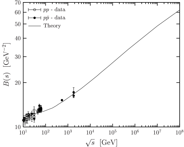
Figure 9: The elastic slope parameter $B(s)$ is shown as a function of the c.m. energy $\sqrt{s}$ for $pp$ and $p{\bar{p}}$ forward ($t=0$) scattering. The solid line represents the model result that is compared with the data for $pp$ (open circles) and $p{\bar{p}}$ (closed circles) reactions from [73, 74, 75].

As expected from the opacity independence of the slope parameter (5.11), saturation effects as seen in the total cross sections do not occur. Indeed, one observes an approximate $B(s)\propto R^{2}(s)\propto\ln^{2}(\sqrt{s}/\sqrt{s_{0}})$ growth for $\sqrt{s}\gtrsim 10^{4}\,\mbox{GeV}$. This behavior agrees, of course, with the transverse expansion of $J_{pp}(s,|\vec{b}_{\!\perp}|)$ for increasing $\sqrt{s}$ shown in Fig. 2. Analogous results are obtained also for $\pi p$ and $Kp$ scattering.

For the good agreement of our model with the data, the finite width of the longitudinal quark momentum distribution in the hadrons, i.e. $\Delta z_{p},\,\Delta z_{\pi},\,\mbox{and}\,\Delta z_{K}\neq 0$ in (A.1), is important as the numerator in (5.11) depends on this width. In fact, $B(s)$ comes out more than 10% smaller with $\Delta z_{p},\,\Delta z_{\pi},\,\mbox{and}\,\Delta z_{K}=0$. Furthermore, a strong growth of the perturbative component, $\epsilon^{P}=0.73$, is important to achieve the increase of $B(s)$ for $\sqrt{s}\gtrsim 500\,\mbox{GeV}$ indicated by the data.

It must be emphasized that only the simultaneous fit of the total cross section and the slope parameter provides the correct shape of the profile function $J(s,|\vec{b}_{\!\perp}|)$. This shape leads then automatically to a good description of the differential elastic cross section $d\sigma^{el}/dt(s,t)$ as demonstrated below. Astonishingly, only few phenomenological models provide a satisfactory description of both quantities [62, 35]. In the approach of [14], for example, the total cross section is described correctly while the slope parameter exceeds the data by more than 20% already at $\sqrt{s}=23.5\,\mbox{GeV}$ and, thus, indicates deficiencies in the form of $J(s,|\vec{b}_{\!\perp}|)$.

5.4 The Differential Elastic Cross Section

The differential elastic cross section obtained from the squared absolute value of the $T$-matrix element

$$\frac{d\sigma^{el}}{dt}(s,t)=\frac{1}{16\pi s^{2}}|T(s,t)|^{2}$$ (5.12)

can be expressed for our purely imaginary $T$-matrix (2.66) in terms of the profile function

$$\frac{d\sigma^{el}}{dt}(s,t)=\frac{1}{4\pi}\left[\int\!\!d^{2}b_{\!\perp}\,e^{i{\vec{q}}_{\!\perp}{\vec{b}}_{\!\perp}}\,J(s,|\vec{b}_{\!\perp}|)\right]^{2}\ .$$ (5.13)

and is, thus, very sensitive to the transverse extension and opacity of the scattered particles. Equation (5.13) reminds of optical diffraction, where $J(s,|\vec{b}_{\!\perp}|)$ describes the distribution of an absorber that causes the diffraction pattern observed for incident plane waves.

In Fig. 10, the differential elastic cross section computed for $pp$ and $p{\bar{p}}$ scattering (solid line) is shown as a function of $|t|=\vec{q}_{\!\perp}^{2}$ at $\sqrt{s}=23.5,\,30.7,\,44.7,\,63,\,546$, and $1800\,\mbox{GeV}$ and compared with experimental data (open circles), where the $pp$ data at $\sqrt{s}=23.5,\,30.7,\,44.7,\,\mbox{and}\,63\,\mbox{GeV}$ were measured at the CERN ISR [64], the $p{\bar{p}}$ data at $\sqrt{s}=546\,\mbox{GeV}$ at the CERN $Sp{{\bar{p}}}S$ [74], and the $p{\bar{p}}$ data at $\sqrt{s}=1.8\,\mbox{TeV}$ at the Fermilab Tevatron [75, 76]. The prediction of our model for the $pp$ differential elastic cross section at the CERN LHC, $\sqrt{s}=14\,\mbox{TeV}$, is given in Fig. 11.

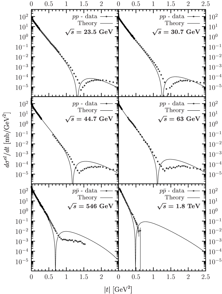
Figure 10: The differential elastic cross section for $pp$ and $p{\bar{p}}$ scattering is shown as a function of $|t|$ up to $2.5\,\mbox{GeV}^{2}$. The result of our model, indicated by the solid line, is compared for $\sqrt{s}=23.5,\,30.7,\,44.7,\,\mbox{and}\,63\,\mbox{GeV}$ with the CERN ISR $pp$ data [64], for $\sqrt{s}=546\,\mbox{GeV}$ with the CERN $Sp{{\bar{p}}}S$ $p{\bar{p}}$ data [74], and for $\sqrt{s}=1.8\,\mbox{TeV}$ with the Fermilab Tevatron $p{\bar{p}}$ data [75, 76], all indicated by the open circles with error bars.

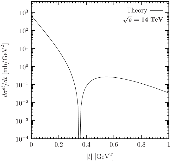
Figure 11: The prediction of our model for the $pp$ differential elastic cross section at LHC ($\sqrt{s}=14\,\mbox{TeV}$) is shown as a function of momentum transfer $|t|$ up to $1\,\mbox{GeV}^{2}$.

For all energies, the model reproduces the experimentally observed diffraction pattern, i.e the characteristic diffraction peak at small $|t|$ and the dip structure at medium $|t|$. As the energy increases, also the shrinking of the diffraction peak is described which reflects the rise of the slope parameter $B(s,t=0)$ already discussed above. The shrinking of the diffraction peak comes along with a dip structure that moves towards smaller values of $|t|$ as the energy increases. This motion of the dip is also described approximately.

The dip in the theoretical curves reflects a change of sign in the $T$-matrix element (2.66). As the latter is purely imaginary, it is not surprising that there are deviations from the data in the dip region. Here, the real part is expected to be important [76] which is in the small $|t|$ region negligible in comparison to the imaginary part.

The difference between the $pp$ and $p{\bar{p}}$ data, a deep dip for $pp$ but only a bump or shoulder for $p{\bar{p}}$ reactions, requires a $C=-1$ contribution. Besides the reggeon contribution at small energies, one expects here an additional perturbative $C=-1$ contribution such as three-gluon exchange [77, 78] or an odderon [79, 80, 81]. In fact, allowing a finite size diquark in the (anti-)proton an odderon appears that supports the dip in $pp$ but leads to the shoulder in $p{\bar{p}}$ reactions [81].

For the differential elastic cross section at the LHC energy, $\sqrt{s}=14\,\mbox{TeV}$, the above findings suggest an accurate prediction in the small-$|t|$ region but a dip at a position smaller than the predicted value at $|t|\approx 0.35\,\mbox{GeV}^{2}$. Our confidence in the validity of the model at small $|t|$ is supported additionally by the total cross section that fixes $d\sigma^{el}/dt(s,t=0)$ and is in agreement with the cosmic ray data shown in Fig. 6. Concerning our prediction for the dip position, it is close to the value $|t|\approx 0.41\,\mbox{GeV}^{2}$ of [62] but significantly below the value $|t|\approx 0.55\,\mbox{GeV}^{2}$ of [14]. Beyond the dip position, the height of the computed shoulder is always above the data and, thus, very likely to exceed also the LHC data. In comparison with other works, the height of our shoulder is similar to the one of [62] but almost one order of magnitude above the one of [14].

Considering Figs. 10 and 11 more quantitatively in the small-$|t|$ region, one can use the well known parametrization of the differential elastic cross section in terms of the slope parameter $B(s)$ and the curvature $C(s)$

$$d\sigma^{el}/dt(s,t)=d\sigma^{el}/dt(s,t=0)\,\exp\left[B(s)t+C(s)t^{2}\right]\ .$$ (5.14)

Using $B(s)$ from the preceding section and assuming for the moment $C(s)=0$, one achieves a good description at small momentum transfers and energies, which is consistent with the approximate Gaussian shape of $J_{pp}(s,|\vec{b}_{\!\perp}|)$ at small energies shown in Fig. 2. The dip, of course, is generated by the deviation from the Gaussian shape at small impact parameters. According to (5.14), the shrinking of the diffraction peak with increasing energy reflects simply the increasing interaction radius described by $B(s)$.

For small energies $\sqrt{s}$, our model reproduces the experimentally observed change in the slope at $|t|\approx 0.25\,\mbox{GeV}^{2}$ [82] that is characterized by a positive curvature. For LHC, we find clearly a negative value for the curvature in agreement with [62] but in contrast to [14]. The change of sign in the curvature reflects the transition of $J(s,|\vec{b}_{\!\perp}|)$ from the approximate Gaussian shape at low energies to the approximate step-function shape (5.4) at high energies.

Important for the good agreement with the data is the longitudinal quark momentum distribution in the proton. Besides the slope parameter, which characterizes the diffraction peak, also the dip position is very sensitive to the distribution width $\Delta z_{p}$, i.e. with $\Delta z_{p}=0$ the dip position appears at more than 10% lower values of $|t|$. In the earlier SVM approach [14], the reproduction of the correct dip position was possible without the $z$-dependence of the hadronic wave functions but a deviation from the data in the low-$|t|$ region had to be accepted. In this low-$|t|$ region, we achieved a definite improvement with the new correlation functions (2.34) and the minimal surfaces used in our model.

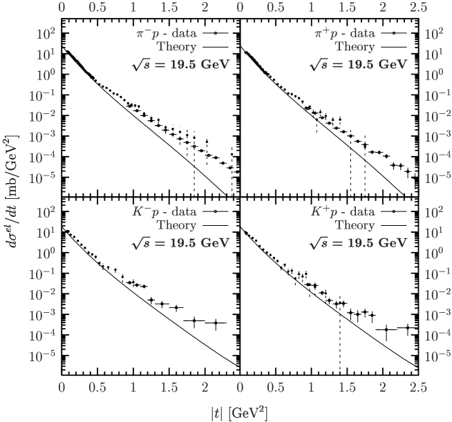
Figure 12: The differential elastic cross section $d\sigma^{el}/dt(s,t)$ is shown versus the momentum transfer $|t|$ for $\pi^{\pm}p$ and $K^{\pm}p$ reactions at the c.m. energy $\sqrt{s}=19.5$ GeV. The model results (solid line) are compared with the data (closed circles with error bars) from [83].

The differential elastic cross section computed for $\pi^{\pm}p$ and $K^{\pm}p$ reactions has the same behavior as the one for $pp$ ($p{\bar{p}}$) reactions. The only difference comes from the different $z$-distribution widths, $\Delta z_{\pi}$ and $\Delta z_{K}$, and the smaller extension parameters, $S_{\pi}$ and $S_{K}$, which shift the dip position to higher values of $|t|$. This is illustrated in Fig. 12, where the model results (solid line) for the $\pi^{\pm}p$ and $K^{\pm}p$ differential elastic cross section as a function of $|t|$ are shown at $\sqrt{s}=19.5\,\mbox{GeV}$ in comparison with experimental data (closed circles) from [83]. The deviations from the data towards large $|t|$ leave room for odderon and reggeon contributions. Indeed, with a finite diquark size in the proton, an odderon occurs that improves the description of the data at large values of $|t|$ [84].

5.5 The Elastic Cross Section $\sigma^{el}$, $\sigma^{el}/\sigma^{tot}$, and $\sigma^{tot}/B$

The elastic cross section obtained by integrating the differential elastic cross section

$$\sigma^{el}(s)=\int_{0}^{-\infty}\!dt\,\frac{d\sigma^{el}}{dt}(s,t)=\int_{0}^{-\infty}\!dt\,\frac{1}{16\pi s^{2}}|T(s,t)|^{2}$$ (5.15)

reduces for our purely imaginary $T$-matrix (2.66) to

$$\sigma^{el}(s)=\int\!\!d^{2}b_{\!\perp}\,|J(s,|\vec{b}_{\!\perp}|)|^{2}\ .$$ (5.16)

Due to the squaring, it exhibits the saturation of $J(s,|\vec{b}_{\!\perp}|)$ at the black disc limit more clearly than $\sigma^{tot}(s)$. Even more transparent is the saturation in the following ratios given here for a purely imaginary $T$-matrix

$$\frac{\sigma^{el}}{\sigma^{tot}}(s) = \frac{\int\!d^{2}b_{\!\perp}\,|J(s,|\vec{b}_{\!\perp}|)|^{2}}{2\int\!d^{2}b_{\!\perp}\,J(s,|\vec{b}_{\!\perp}|)}\ ,$$ (5.17)

$$\frac{\sigma^{tot}}{B}(s) = \frac{\left(2\int\!d^{2}b_{\!\perp}\,J(s,|\vec{b}_{\!\perp}|)\right)^{2}}{\int\!d^{2}b_{\!\perp}\,|\vec{b}_{\!\perp}|^{2}\,J(s,|\vec{b}_{\!\perp}|)}\ ,$$ (5.18)

which are directly sensitive to the opacity of the particles. This sensitivity can be illustrated within the approximation

$$T(s,t)=i\,s\,\sigma^{tot}(s)\,\exp[B(s)t/2]$$ (5.19)

that leads to the differential cross section (5.14) with $C(s)=0$, i.e. an exponential decrease over $|t|$ with a slope $B(s)$. As the purely imaginary $T$-matrix element (5.19) is equivalent to

$$J(s,|\vec{b}_{\!\perp}|)=(\sigma^{tot}/4\pi B)\,\exp[-|\vec{b}_{\!\perp}|^{2}/2B]=(4\sigma^{el}/\sigma^{tot})\,\exp[-|\vec{b}_{\!\perp}|^{2}/2B]\ ,$$ (5.20)

one finds that the above ratios are a direct measure for the opacity at zero impact parameter

$$J(s,|\vec{b}_{\!\perp}|=0)=(\sigma^{tot}/4\pi B)=(4\sigma^{el}/\sigma^{tot})\ .$$ (5.21)

For a general purely imaginary $T$-matrix, $T(s,t)=i\,s\,\sigma^{tot}\,g(|t|)$ with an arbitrary real-valued function $g(|t|)$, $J(s,|\vec{b}_{\!\perp}|=0)$ is given by $(\sigma^{el}/\sigma^{tot})$ times a pure number which depends on the shape of $g(|t|)$.

We compute the elastic cross section $\sigma^{el}$ and the ratios $\sigma^{el}/\sigma^{tot}$ and $\sigma^{tot}/B$ in our model without taking into account reggeons. In Fig. 13, the results for $pp$ and $p{\bar{p}}$ reactions (solid lines) are compared with the experimental data (open and closed circles). The data for the elastic cross section are taken from [1] and the data for $\sigma^{tot}$ and $B$ from the references given in previous sections.

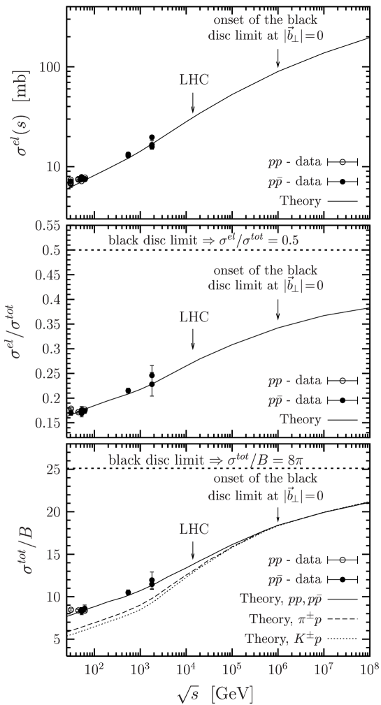
Figure 13: The elastic cross section $\sigma^{el}$ and the ratios $\sigma^{el}/\sigma^{tot}$ and $\sigma^{tot}/B$ are shown as a function of the c.m. energy $\sqrt{s}$. The model results for $pp$ ($p{\bar{p}}$), $\pi p$, and $Kp$ scattering are represented by the solid, dashed and dotted lines, respectively. The experimental data for the $pp$ and $p{\bar{p}}$ reactions are indicated by the open and closed circles, respectively. The data for the elastic cross section are taken from [1] and the data for $\sigma^{tot}$ and $B$ from the references given in previous sections.

For $pp$ ($p{\bar{p}}$) scattering, we indicate explicitly the prediction for LHC at $\sqrt{s}=14\,\mbox{TeV}$ and the onset of the black disc limit at $\sqrt{s}=10^{6}\,\mbox{GeV}$. The model results for $\pi p$ and $Kp$ reactions are presented as dashed and dotted line, respectively. For the ratios, the asymptotic limits are indicated: Since the maximum opacity or black disc limit governs the $\sqrt{s}\to\infty$ behavior, $\sigma^{el}/\sigma^{tot}$ ($\sigma^{tot}/B$) cannot exceed $0.5$ ($8\pi$) in hadron-hadron scattering.

In the investigation of $pp$ ($p{\bar{p}}$) scattering, our theoretical curves confront successfully the experimental data for the elastic cross section and both ratios. At low energies, the data are underestimated as reggeon contributions are not taken into account. Again, the agreement is comparable to the one achieved in [62] and better than in the approach of [14], where $\sigma^{el}$ comes out too small due to an underestimation of $d\sigma^{el}/dt$ in the low-$|t|$ region.

Concerning the energy dependence, $\sigma^{el}$ shows a similar behavior as $\sigma^{tot}$ but with a more pronounced flattening around $\sqrt{s}\gtrsim 10^{6}\,\mbox{GeV}$. This flattening is even stronger for the ratios, drawn on a linear scale, and reflects very clearly the onset of the black disc limit. As expected from the simple approximation (5.21), $\sigma^{el}/\sigma^{tot}$ and $\sigma^{tot}/B$ show a similar functional dependence on $\sqrt{s}$. At the highest energy shown, $\sqrt{s}=10^{8}\,\mbox{GeV}$, both ratios are still below the indicated asymptotic limits, which reflects that $J(s,|\vec{b}_{\!\perp}|)$ still deviates from the step-function shape (5.4). The ratios $\sigma^{el}/\sigma^{tot}$ and $\sigma^{tot}/B$ reach their upper limits $0.5$ and $8\pi$, respectively, at asymptotic energies, $\sqrt{s}\to\infty$, where the hadrons become infinitely large, completely black discs.

Comparing the $pp$ ($p{\bar{p}}$) results with the ones for $\pi p$ and $Kp$, one finds that the results for $\sigma^{tot}/B$ converge at high energies as shown in Fig. 13. This follows from the identical normalizations of the hadron wave functions that lead to an identical black disc limit for hadron-hadron reactions.

6 Conclusion

We have developed a loop-loop correlation model combining perturbative and non-perturbative QCD to compute high-energy reactions of hadrons and photons. We have aimed at a unified description of hadron-hadron, photon-hadron, and photon-photon reactions involving real and virtual photons as well. Being particularly interested in saturation effects that manifest the $S$-matrix unitarity, we have investigated the scattering amplitudes in impact parameter space since the black disc limit of the profile function is the most explicit signature of unitarity. Using a leading twist, next-to-leading order DGLAP relation, we have also estimated the impact parameter dependent gluon distribution of the proton $xG(x,Q^{2},|\vec{b}_{\perp}|)$ to study gluon saturation as a manifestation of the $S$-matrix unitarity at small Bjorken $x$. In addition, the calculated profile functions provide an intuitive geometrical picture for the energy dependence of the cross sections and allow us to localize saturation effects in the experimental observables.

Following the functional integral approach to high-energy scattering in the eikonal approximation [10, 11, 12, 13], the scattering hadrons and photons are described by light-like Wegner-Wilson loops (color-dipoles) with size and orientation weighted with appropriate light-cone wave functions [12]. The resulting $S$-matrix element factorizes into the universal correlation of two light-like Wegner-Wilson loops $S_{DD}$ (loop-loop correlation function) and reaction-specific light-cone wave functions. This factorization has allowed us to provide a unified description of hadron-hadron, photon-hadron, and photon-photon scattering. We have used for hadrons the phenomenological Gaussian wave function [25, 26] and for photons the perturbatively derived wave function with running quark masses $m_{f}(Q^{2})$ to account for the non-perturbative region of low photon virtuality $Q^{2}$ [22].

The loop-loop correlation function $S_{DD}$ has been computed in the approach of Berger and Nachtmann [14]. The loop-loop correlation function $S_{DD}$ has been expressed in terms of surface ($S_{1,2}$) integrals over the gauge-invariant bilocal gluon field strength correlator. We have divided this correlator into a non-perturbative and a perturbative component. The stochastic vacuum model (SVM) [15] has been used for the non-perturbative low frequency background field (long-distance correlations) and perturbative gluon exchange for the additional high frequency contributions (short-distance correlations) since this combination is supported by lattice investigations of the gluon field strength correlator [18, 19]. The exponential correlation function used in the non-perturbative component has been adopted directly from a lattice investigation of the correlator [19]. Since this correlation function stays positive for all Euclidean distances, it is compatible with a spectral representation of the correlation function [20], which means a conceptual improvement since the correlation function that has been used in earlier applications of the SVM becomes negative at large distances [12, 21, 22, 23, 24, 14, 25]. We have presented for the first time an explicit computation of the surface integrals using minimal surfaces ($S_{1,2}$) bounded by the Wegner-Wilson loops. This surface choice is usually used to obtain Wilson’s area law in Euclidean space [15, 16]. Moreover, the simplicity of the minimal surfaces has allowed us to identify very clearly a string-string interaction in the non-perturbative component.

The strongest assumption in the presented work is the form of the energy dependence introduced phenomenologically into the loop-loop correlation function $S_{DD}$. Motivated by the two-pomeron model of Donnachie and Landshoff [6], we have ascribed to the non-perturbative and to the perturbative component a weak and a strong energy dependence, respectively. The constructed $T$-matrix element shows Regge behavior at moderately high energies and contains multiple gluonic interactions important to respect unitarity in impact parameter space at ultra-high energies.

The model parameters have been adjusted to reproduce a wealth of experimental data (including cosmic ray data) over a large range of c.m. energies: total, differential, and elastic cross sections, structure functions, and slope parameters — including cosmic ray data. The model parameters that allowed a good fit to high-energy scattering data are in good agreement with complementary investigations: The parameters of the non-perturbative component — the correlation length $a$, the non-Abelian strength $\kappa$, and the gluon condensate $G_{2}$ — are constrained by lattice QCD investigations, by the string tension $\sigma$ of a static quark-antiquark pair, and by the SVZ gluon condensate $G_{2}$ essential in QCD sum rule investigations. The parameters of the perturbative component have not been adjusted. We have used the $\rho$-meson mass for the effective gluon mass $m_{G}$ representing the IR regulator and have determined $M^{2}$ so that the strong coupling freezes for large distance scales at $\alpha_{s}=0.4$, where our non-perturbative component is at work according to a low energy theorem [33, 16]. For the energy dependence, the exponents of the Donnachie-Landshoff two-pomeron fit, $\epsilon_{soft}$ and $\epsilon_{hard}$, have been used as an orientation for our energy exponents $\epsilon^{N\!P}$ and $\epsilon^{P}$. Besides these parameters describing the universal loop-loop correlation function $S_{DD}$, the reaction-dependent parameters in the light-cone wave functions are also consistent with other approaches: In the hadron wave functions, the transverse extension parameters $S_{h}$ have been found in good agreement with the corresponding electromagnetic radii [25] while the width of the longitudinal quark momentum distributions $\Delta z_{h}$ has been computed from [26]. In the photon wave function, the running quark masses that coincide with the current quark masses for large $Q^{2}$ and the constituent quark masses for small $Q^{2}$ [22] have been chosen in agreement with sum rule derivations.

Having adjusted the model parameters, we have studied $S$-matrix unitarity limits of the scattering amplitudes in impact parameter space. On the basis of dipole-dipole scattering, we have found explicitly that our model preserves the unitarity condition and attains the black disc limit at ultra-high energies. The profile functions have been calculated for proton-proton and photon-proton scattering and have shown very clearly that the interacting particles become blacker and larger with increasing energy. At ultra-high energies, the opacity saturates at the black disc limit while the transverse expansion of the scattered particles continues. Moreover, in longitudinal photon-proton scattering, we have observed that with increasing photon virtuality $Q^{2}$ not only the maximum opacity increases but also the energy at which it is reached for zero impact parameter.

Using a leading twist, next-to-leading order QCD relation between the gluon distribution of the proton $xG(x,Q^{2})$ and the longitudinal proton structure function $F_{L}(x,Q^{2})$ [48, 49], we have related the impact parameter dependent gluon distribution $xG(x,Q^{2},|\vec{b}_{\perp}|)$ to the profile function for longitudinal photon-proton scattering and found low-$x$ saturation of $xG(x,Q^{2},|\vec{b}_{\perp}|)$ as a manifestation of $S$-matrix unitarity. In accordance with the profile function, $xG(x,Q^{2},|\vec{b}_{\perp}|)$ decreases from the center towards the periphery of the proton. With increasing photon virtuality $Q^{2}$, the increase of $xG(x,Q^{2},|\vec{b}_{\perp}|=0)$ becomes stronger towards small $x$ and the saturation value of $xG(x,Q^{2},|\vec{b}_{\perp}|=0)$ increases but is reached at decreasing values of $x$. In contrast, at fixed $Q^{2}$, the integrated gluon distribution $xG(x,Q^{2})$ does not saturate because of the growth of the proton radius with decreasing $x$ observed in our approach. Similar results are obtained in complementary approaches [47, 50, 51].

More model dependent are the specific energies where these saturation effects set in. The profile function saturates the black disc limit at zero impact parameter for $\sqrt{s}\gtrsim 10^{6}\,\mbox{GeV}$ in proton-proton scattering and for $\sqrt{s}\gtrsim 10^{7}\,\mbox{GeV}$ in longitudinal photon-proton scattering with $Q^{2}\gtrsim 1\,\mbox{GeV}^{2}$. In both reactions, the wave function normalization determines the maximum opacity. The saturation of $xG(x,Q^{2},|\vec{b}_{\perp}|)$ occurs in our approach for $Q^{2}\gtrsim 1\,\mbox{GeV}^{2}$ at values of $x\lesssim 10^{-10}$, far below the HERA and THERA range.

For proton-proton scattering, we have observed that the rise of the total and elastic cross section becomes weaker for $\sqrt{s}\gtrsim 10^{6}\,\mbox{GeV}$ due to the onset of the black disc limit at $|\vec{b}_{\perp}|=0$ in the profile function. This saturation of the profile function has become even more apparent in the ratios $\sigma^{el}/\sigma^{tot}$ and $\sigma^{tot}/B$ which are a measure of the proton opacity. In contrast, no saturation effect has been observed in the slope parameter $B(s)$ which is a measure of the transverse expansion of the proton. Considering the differential elastic cross section $d\sigma^{el}/dt$, the model has described the diffraction pattern and also the shrinkage of the diffraction peak with increasing energy in good agreement with experimental data at small momentum transfers $|t|$. Around the dip region, where a real part is expected to be important, deviations from the data have reflected that our $T$-matrix is purely imaginary. Our predictions for proton-proton scattering at LHC ($\sqrt{s}=14\,\mbox{TeV}$) have been a total cross section of $\sigma^{tot}_{pp}=114.2\,\mbox{mb}$ in good agreement with the cosmic ray data and a differential elastic cross section $d\sigma^{el}/dt$ with a slope parameter of $B=21.26\,\mbox{GeV}^{-2}$, a negative curvature, $C<0$, and a dip at $|t|\approx 0.35\,\mbox{GeV}^{2}$.

For pion-proton and kaon-proton scattering, results analogous to proton-proton scattering have been obtained but with a slightly stronger rise observed in the total cross section. This has been traced back to the smaller size of pions and kaons in comparison to protons, $S_{p}=0.86\,\mbox{fm}>S_{\pi}=0.607\,\mbox{fm}>S_{K}=0.55\,\mbox{fm}$, and the perturbative component becoming increasingly important with decreasing dipole sizes involved. Furthermore, a weak convergence of the ratios $\sigma^{tot}_{pp}/\sigma^{tot}_{\pi p}$ and $\sigma^{tot}_{pp}/\sigma^{tot}_{Kp}$ towards unity has been observed as the energy increases. The smaller size of the pion and kaon has also been reflected in the differential elastic cross sections $d\sigma^{el}/dt$, where the dip is shifted towards larger values of $|t|$.

For photon-proton and photon-photon reactions, an even stronger rise of the total cross section has been observed with increasing energy. As illustrated in the proton structure function $F_{2}(x,Q^{2})$, this rise becomes steeper with increasing photon virtuality $Q^{2}$. Again, we have traced back the strong energy boost to the growing importance of the perturbative component with decreasing dipole size. Besides some deviations from the experimental data with increasing $Q^{2}$, our model has described $\sigma^{tot}_{\gamma^{*}p}(s,Q^{2})$ successfully in the low-$Q^{2}$ region where the running quark masses become constituent quark masses.

We plan to present complementary investigations within our model in future work. Going to momentum space, we calculate on the two-gluon exchange level the unintegrated gluon distribution of the proton. Insight into the non-perturbative structure of this distribution can be gained from the non-perturbative component of our model [17]. In Euclidean space-time, we compute the static quark-antiquark potential, the associated flux tube, and the van der Waals force between two static color-dipoles [16]. It is a long-range project to implement the energy dependence more fundamentally. In a recent attempt, the energy dependence of high-energy scattering has been related successfully to critical properties of an effective near light-cone Hamiltonian in a non-perturbative lattice approach [85]. Furthermore, the correlation of inclined Euclidean Wegner-Wilson loops generates energy dependence after analytic continuation to Minkowski space-time [86]. Here, encouraging new results obtained with instantons [87] and within the AdS/CFT correspondence [88] have to be compared to calculations in the stochastic vacuum model.

Appendix A Hadron and Photon Wave Functions

The light-cone wave functions $\psi_{i}(z_{i},\vec{r}_{i})$ provide the distribution of transverse size and orientation ${\vec{r}}_{i}$ and longitudinal quark momentum fraction $z_{i}$ to the light-like Wegner-Wilson loops $W[C_{i}]$ that represent the scattering color-dipoles. In this way, they specify the projectiles as mesons, baryons described as quark-diquark systems, or photons that fluctuate into a quark-antiquark pair before the interaction.

The Hadron Wave Function

In this work, mesons and baryons are assumed to have a quark-antiquark and quark-diquark valence structure, respectively. As quark-diquark systems are equivalent to quark-antiquark systems [89], this allows us to model not only mesons but also baryons as color-dipoles represented by Wegner-Wilson loops. To characterize mesons and baryons, we use the phenomenological Gaussian Wirbel-Stech-Bauer ansatz [26]

$$\psi_{h}(z_{i},\vec{r}_{i})=\sqrt{\frac{z_{i}(1-z_{i})}{2\pi S_{h}^{2}N_{h}}}\,e^{-(z_{i}-\frac{1}{2})^{2}/(4\Delta z_{h}^{2})}\,e^{-|\vec{r}_{i}|^{2}/(4S_{h}^{2})}\ ,$$ (A.1)

where the hadron wave function normalization to unity

$$\int\!\!dz_{i}d^{2}r_{i}\ |\psi_{i}(z_{i},\vec{r}_{i})|^{2}=1\ ,$$ (A.2)

requires the normalization constant

$$N_{h}=\int_{0}^{1}dz_{i}\ z_{i}(1-z_{i})\ e^{-(z_{i}-\frac{1}{2})^{2}/(2\Delta z_{h}^{2})}\ .$$ (A.3)

The different hadrons considered — protons, pions, and kaons — are specified by $\Delta z_{h}$ and $S_{h}$ providing the width for the distributions of the longitudinal momentum fraction carried by the quark $z_{i}$ and transverse spatial extension $|\vec{r}_{i}|$, respectively. In this work, the extension parameter $S_{h}$ is a fit parameter that should resemble approximately the electromagnetic radius of the corresponding hadron [25], while $\Delta z_{h}=w/(\sqrt{2}\,m_{h})$ [26] is fixed by the hadron mass $m_{h}$ and the value $w=0.35-0.5\,\mbox{GeV}$ extracted from experimental data. We find for (anti-)protons $\Delta z_{p}=0.3$ and $S_{p}=0.86\,\mbox{fm}$, for pions $\Delta z_{\pi}=2$ and $S_{\pi}=0.607\,\mbox{fm}$, and for kaons $\Delta z_{K}=0.57$ and $S_{K}=0.55\,\mbox{fm}$ which are the values used in the main text. For convenience they are summarized in Table 1.

Table 1: Hadron Parameters

Hadron	$\Delta z_{h}$	$S_{h}\;[\mbox{fm}]$
$p,\bar{p}$	$0.3$	$0.86$
$\pi^{\pm}$	$2$	$0.607$
$K^{\pm}$	$0.57$	$0.55$

Concerning the quark-diquark structure of the baryons, the more conventional three-quark structure of a baryon would complicate the model significantly but would lead to similar predictions once the model parameters are readjusted [12]. In fact, there are also physical arguments that favor the quark-diquark structure of the baryon such as the $\delta I=1/2$ enhancement in semi-leptonic decays of baryons [89] and the strong attraction in the scalar diquark channel in the instanton vacuum [90].

The Photon Wave Function

The photon wave function $\psi_{\gamma}(z_{i},\vec{r}_{i},Q^{2})$ describes the fluctuation of a photon with virtuality $Q^{2}$ into a quark-antiquark pair with longitudinal quark momentum fraction $z_{i}$ and spatial transverse size and orientation $\vec{r}_{i}$. The computation of the corresponding transition amplitude $\langle q{\bar{q}}(z_{i},\vec{r}_{i})|\gamma^{*}(Q^{2})\rangle$ can be performed conveniently in light-cone perturbation theory [91] and leads to the following squared wave functions for transverse $(T)$ and longitudinally $(L)$ polarized photons [34]

$$\!\!\!\!\!\!\!\!\!\!\!\!\!|\psi_{\gamma_{T}^{*}}(z_{i},\vec{r}_{i},Q^{2})|^{2}\! \!\!=\!\! \!\frac{3\,\alpha}{2\,\pi^{2}}\sum_{f}e_{f}^{2}\left\{\left[z_{i}^{2}+(1-z_{i})^{2}\right]\,\epsilon_{f}^{2}\,K_{1}^{2}(\epsilon_{f}\,|\vec{r}_{i}|)+m_{f}^{2}\,K_{0}^{2}(\epsilon_{f}\,|\vec{r}_{i}|)\right\}$$ (A.4)

$$\!\!\!\!\!\!\!\!\!\!\!\!\!|\psi_{\gamma_{L}^{*}}(z_{i},\vec{r}_{i},Q^{2})|^{2}\! \!\!=\!\! \!\frac{3\,\alpha}{2\,\pi^{2}}\sum_{f}e_{f}^{2}\left\{4\,Q^{2}\,z_{i}^{2}(1-z_{i})^{2}\,K_{0}^{2}(\epsilon_{f}\,|\vec{r}_{i}|)\right\},$$ (A.5)

where $\alpha$ is the fine-structure constant, $e_{f}$ is the electric charge of the quark with flavor $f$, and $K_{0}$ and $K_{1}$ are the modified Bessel functions (McDonald functions). In the above expressions,

$$\epsilon_{f}^{2}=z_{i}(1-z_{i})\,Q^{2}+m_{f}^{2}$$ (A.6)

controlls the transverse size(-distribution) of the emerging dipole, $|\vec{r}_{i}|\propto 1/\epsilon_{f}$, that depends on the quark flavor through the current quark mass $m_{f}$.

For small $Q^{2}$, the perturbatively derived wave functions, (A.4) and (A.5), are not appropriate since the resulting large color-dipoles, i.e. $|\vec{r}_{i}|\propto 1/m_{f}\gg 1\,\mbox{fm}$, should encounter non-perturbative effects such as confinement and chiral symmetry breaking. To take these effects into account the vector meson dominance (VMD) model [92] is usually used. However, the transition from the “partonic” behavior at large $Q^{2}$ to the “hadronic” one at small $Q^{2}$ can be modelled as well by introducing $Q^{2}$-dependent quark masses, $m_{f}=m_{f}(Q^{2})$, that interpolate between the current quarks at large $Q^{2}$ and the constituent quarks at small $Q^{2}$ [22]. Following this approach, we use (A.4) and (A.5) also in the low-$Q^{2}$ region but with the running quark masses

$$m_{u,d}(Q^{2}) = 0.178\,\mbox{GeV}\,(1-\frac{Q^{2}}{Q^{2}_{u,d}})\,\Theta(Q^{2}_{u,d}-Q^{2})\ ,$$ (A.7)

$$m_{s}(Q^{2}) = 0.121\,\mbox{GeV}+0.129\,\mbox{GeV}\,(1-\frac{Q^{2}}{Q^{2}_{s}})\,\Theta(Q^{2}_{s}-Q^{2})\ ,$$ (A.8)

and the fixed charm quark mass

$$m_{c}=1.25\,\mbox{GeV}\ ,$$ (A.9)

where the parameters $Q^{2}_{u,d}=1.05\,\mbox{GeV}^{2}$ and $Q^{2}_{s}=1.6\,\mbox{GeV}^{2}$ are taken directly from [22] while we reduced the values for the constituent quark masses $m_{f}(Q^{2}=0)$ of [22] by about 20%. The smaller constituent quark masses are necessary in order to reproduce the total cross sections for $\gamma^{*}p$ and $\gamma^{*}\gamma^{*}$ reactions at low $Q^{2}$. Similar running quark masses are obtained in a QCD-motivated model of the spontaneous chiral symmetry breaking in the instanton vacuum [93] that improve the description of $\gamma^{*}p$ scattering at low $Q^{2}$ [94].

Appendix B Correlation Functions

In this Appendix, we describe explicitly the way from the simple exponential correlation functions in Euclidean space-time (2.34) to their transverse Fourier transforms in Minkowski space-time, (2.50) and (2.55). The first step in this procedure is the Fourier transformation of the exponential correlation functions (2.34) in four-dimensional Euclidean space-time

$$\tilde{D}^{E}(K^{2}) \!=\! \tilde{D}^{E}_{1}(K^{2})=\int\!d^{4}Z\,D^{E}(Z^{2}/a^{2})\,e^{iKZ}$$ (B.1)

$$\!=\! \int_{0}^{\infty}\!\!\!d|Z|\,|Z|^{3}\int_{0}^{\pi}\!\!\!d\phi_{3}\,\sin^{2}\!\phi_{3}\int_{0}^{\pi}\!\!\!d\phi_{2}\,\sin\!\phi_{2}\int_{0}^{2\pi}\!\!\!d\phi_{1}\,D^{E}(Z^{2}/a^{2})\,e^{-i|K||Z|\cos\!\phi_{3}}$$

$$\!=\! \frac{4\pi^{2}}{|K|}\int_{0}^{\infty}\!\!\!d|Z|\,|Z|^{2}\,D^{E}(Z^{2}/a^{2})\,J_{1}(|K||Z|)\,=\,\frac{12\pi^{2}}{a\,(K^{2}+a^{-2})^{\frac{5}{2}}}\ ,$$

where $J_{1}$ is the $1st$ order Bessel function of the first kind. Here, the Euclidean metric $-\delta_{\mu\nu}$ and four-dimensional polar coordinates and the corresponding four-volume element $d^{4}Z=d|Z|\,|Z|^{3}\,d\phi_{3}\,\sin^{2}\!\phi_{3}\,d\phi_{2}\,\sin\!\phi_{2}\,d\phi_{1}$ have been used. With (B.1), one obtains

$$\tilde{D}^{\prime\,E}_{1}(K^{2}):=\frac{d}{dK^{2}}\,\tilde{D}^{E}_{1}(K^{2})=-\,\frac{30\pi^{2}}{a\,(K^{2}+a^{-2})^{\frac{7}{2}}}\ .$$ (B.2)

Now, (B.1) and (B.2) are analytically continued to Minkowski space-time, $K_{4}\to ik^{0}$ or equivalently $-\delta_{\mu\nu}\to g_{\mu\nu}=\mbox{diag}(1,-1,-1,-1)$,

$$\tilde{D}(k^{2})=-\,\frac{12\,\pi^{2}\,i}{a\,(-k^{2}+a^{-2})^{\frac{5}{2}}}\ ,\quad\quad\quad\tilde{D}^{\prime}_{1}(k^{2})=-\,\frac{30\,\pi^{2}\,i}{a(-k^{2}+a^{-2})^{\frac{7}{2}}}\ .$$ (B.3)

Setting $k^{0}=k^{3}=0$, which is enforced in the computation of $\chi$ by $\delta$-functions, one finds $k^{2}=-{\vec{k}}^{2}_{\!\perp}$ and consequently

$$\hphantom{-}\tilde{D}^{(2)}({\vec{k}}^{2}_{\!\perp})=-\,\frac{12\,\pi^{2}\,i}{a\,({\vec{k}}^{2}_{\!\perp}+a^{-2})^{\frac{5}{2}}}\ ,\quad\quad\quad\hphantom{-}\tilde{D}^{\prime\,(2)}_{1}({\vec{k}}^{2}_{\!\perp})=-\,\frac{30\,\pi^{2}\,i}{a({\vec{k}}^{2}_{\!\perp}+a^{-2})^{\frac{7}{2}}}\ .$$ (B.4)

The transverse Fourier transformation (2.48) of these two expressions is the remaining step that leads directly to (2.50) and (2.55).

References

- [1] D. E. Groom et al. [Particle Data Group], Eur. Phys. J. C 15 (2000) 1.
- [2] C. Adloff et al. [H1 Collaboration], Nucl. Phys. B 497 (1997) 3; Eur. Phys. J. C 19 (2001) 269; J. Breitweg et al. [ZEUS Collaboration], Phys. Lett. B 407 (1997) 432; Phys. Lett. B 487 (2000) 53.
- [3] C. Adloff et al. [H1 Collaboration], Eur. Phys. J. C 21 (2001) 33.
- [4] J. Breitweg et al. [ZEUS Collaboration], Z. Phys. C 75 (1997) 215; C. Adloff et al. [H1 Collaboration], Phys. Lett. B 483 (2000) 23.
- [5] M. Froissart, Phys. Rev. 123 (1961) 1053; A. Martin, Phys. Rev. 129 (1963) 1432; Nuovo Cim. A 42 (1965) 930; L. Lukaszuk and A. Martin, Nuovo Cim. A 47 (1967) 265.
- [6] A. Donnachie and P. V. Landshoff, Phys. Lett. B 437 (1998) 408; “New data and the hard pomeron,” hep-ph/0105088.
- [7] A. Donnachie and P. V. Landshoff, Phys. Lett. B 296 (1992) 227.
- [8] E. A. Kuraev, L. N. Lipatov and V. S. Fadin, Sov. Phys. JETP 45 (1977) 199 [Zh. Eksp. Teor. Fiz. 72 (1977) 377]; I. I. Balitsky and L. N. Lipatov, Sov. J. Nucl. Phys. 28 (1978) 822 [Yad. Fiz. 28 (1978) 1597].
- [9] K. Golec-Biernat and M. Wüsthoff, Phys. Rev. D 59 (1999) 014017; Phys. Rev. D 60 (1999) 114023.
- [10] O. Nachtmann, Annals Phys. 209 (1991) 436.
- [11] A. Krämer and H. G. Dosch, Phys. Lett. B 252 (1990) 669.
- [12] H. G. Dosch, E. Ferreira and A. Krämer, Phys. Rev. D 50 (1994) 1992.
- [13] O. Nachtmann, in “Perturbative and Nonperturbative Aspects of Quantum Field Theory”, edited by H. Latal and W Schweiger (Springer Verlag, Berlin, Heidelberg 1997) [hep-ph/9609365].
- [14] E. R. Berger and O. Nachtmann, Eur. Phys. J. C 7 (1999) 459.
- [15] H. G. Dosch, Phys. Lett. B 190 (1987) 177; H. G. Dosch and Y. A. Simonov, Phys. Lett. B 205 (1988) 339; Y. A. Simonov, Nucl. Phys. B 307 (1988) 512.
- [16] A. I. Shoshi, F. D. Steffen, H. G. Dosch, and H. J. Pirner, HD-THEP-02-22 (2002).
- [17] A. I. Shoshi, F. D. Steffen, H. G. Dosch, and H. J. Pirner, HD-THEP-02-21 (2002).
- [18] A. Di Giacomo and H. Panagopoulos, Phys. Lett. B 285 (1992) 133; A. Di Giacomo, E. Meggiolaro and H. Panagopoulos, Nucl. Phys. B 483 (1997) 371; M. D’Elia, A. Di Giacomo and E. Meggiolaro, Phys. Lett. B 408 (1997) 315; G. S. Bali, N. Brambilla and A. Vairo, Phys. Lett. B 421 (1998) 265.
- [19] E. Meggiolaro, Phys. Lett. B 451 (1999) 414.
- [20] H. G. Dosch, M. Eidemüller and M. Jamin, Phys. Lett. B 452 (1999) 379.
- [21] M. Rueter and H. G. Dosch, Phys. Lett. B 380 (1996) 177; H. G. Dosch, T. Gousset, G. Kulzinger and H. J. Pirner, Phys. Rev. D 55 (1997) 2602; M. Rueter and H. G. Dosch, Phys. Rev. D 57 (1998) 4097; G. Kulzinger, H. G. Dosch and H. J. Pirner, Eur. Phys. J. C 7 (1999) 73.
- [22] H. G. Dosch, T. Gousset and H. J. Pirner, Phys. Rev. D 57 (1998) 1666.
- [23] M. Rueter, Eur. Phys. J. C 7 (1999) 233.
- [24] U. D’Alesio, A. Metz and H. J. Pirner, Eur. Phys. J. C 9 (1999) 601.
- [25] H. G. Dosch, O. Nachtmann, T. Paulus and S. Weinstock, Eur. Phys. J. C 21 (2001) 339.
- [26] M. Wirbel, B. Stech and M. Bauer, Z. Phys. C 29 (1985) 637.
- [27] F. J. Wegner, J. Math. Phys. 12 (1971) 2259; K. G. Wilson, Phys. Rev. D 10 (1974) 2445.
- [28] N. E. Bralic, Phys. Rev. D 22 (1980) 3090; P. M. Fishbane, S. Gasiorowicz and P. Kaus, Phys. Rev. D 24 (1981) 2324; L. Diosi, Phys. Rev. D 27 (1983) 2552; Y. A. Simonov, Sov. J. Nucl. Phys. 48 (1988) 878 [Yad. Fiz. 48 (1988) 1381].
- [29] N. G. Van Kampen, Physica 74 (1997) 215, 239; Phys. Rep. C24 (1976) 172; A. Y. Dubin and Y. S. Kalashnikova, Phys. Atom. Nucl. 58 (1995) 1967 [Yad. Fiz. 58 (1995) 2078].
- [30] M. A. Shifman, A. I. Vainshtein and V. I. Zakharov, Nucl. Phys. B 147 (1979) 385; Nucl. Phys. B 147 (1979) 448.
- [31] G. S. Bali, Phys. Rept. 343 (2001) 1.
- [32] J. B. Kogut, Rev. Mod. Phys. 51 (1979) 659, Sec. VI.
- [33] M. Rueter and H. G. Dosch, Z. Phys. C 66 (1995) 245; H. G. Dosch, O. Nachtmann and M. Rueter, “String formation in the model of the stochastic vacuum and consistency with low-energy theorems,” hep-ph/9503386.
- [34] N. N. Nikolaev and B. G. Zakharov, Z. Phys. C 49 (1991) 607.
- [35] B. Z. Kopeliovich, I. K. Potashnikova, B. Povh and E. Predazzi, Phys. Rev. D 63 (2001) 054001.
- [36] J. R. Forshaw, G. Kerley and G. Shaw, Phys. Rev. D 60 (1999) 074012.
- [37] A. Donnachie and H. G. Dosch, Phys. Rev. D 65 (2002) 014019.
- [38] For a review on heavy quarkonium phenomenology, see e.g. W. Kwong, J. L. Rosner and C. Quigg, Ann. Rev. Nucl. Part. Sci. 37 (1987) 325.
- [39] P. Goddard, J. Goldstone, C. Rebbi and C. B. Thorn, Nucl. Phys. B 56 (1973) 109; K. Johnson and C. B. Thorn, Phys. Rev. D 13 (1976) 1934.
- [40] U. Amaldi, M. Jacob and G. Matthiae, Ann. Rev. Nucl. Part. Sci. 26 (1976) 385.
- [41] R. Castaldi and G. Sanguinetti, Ann. Rev. Nucl. Part. Sci. 33 (1983) 351.
- [42] L. Van Hove, Rev. Mod. Phys. 36 (1964) 655.
- [43] L. Frankfurt, V. Guzey, M. McDermott and M. Strikman, Phys. Rev. Lett. 87 (2001) 192301; “Electron nucleus collisions at THERA,” hep-ph/0104252.
- [44] P. Desgrolard, L. Jenkovszkii, and B. Struminsky, Eur. Phys. J. C 11 (1999) 144.
- [45] A. D. Martin and M. G. Ryskin, Phys. Lett. B 431 (1998) 395; J. Bartels, K. Golec-Biernat and K. Peters, Eur. Phys. J. C 17 (2000) 121.
- [46] L. V. Gribov, E. M. Levin and M. G. Ryskin, Phys. Rept. 100 (1983) 1.
- [47] A. H. Mueller and J. Qiu, Nucl. Phys. B 268 (1986) 427.
- [48] A. D. Martin, R. G. Roberts and W. J. Stirling, Phys. Rev. D 37 (1988) 1161.
- [49] A. M. Cooper-Sarkar, G. Ingelman, K. R. Long, R. G. Roberts and D. H. Saxon, Z. Phys. C 39 (1988) 281; A. M. Cooper-Sarkar, R. C. Devenish and M. Lancaster, “Measurement of at low , and extraction of the gluon distribution,” in 1992 Proc. Workshop on Physics at HERA vol. 1 (1991) p. 155, ed. W. Buchmüller and G. Ingelman.
- [50] A. H. Mueller, Nucl. Phys. B 558 (1999) 285.
- [51] E. Iancu and L. D. McLerran, Phys. Lett. B 510 (2001) 145.
- [52] E. Gotsman, E. Ferreira, E. Levin, U. Maor and E. Naftali, Phys. Lett. B 500 (2001) 87.
- [53] H. Abramowicz and A. Caldwell, Rev. Mod. Phys. 71 (1999) 1275.
- [54] L. D. McLerran and R. Venugopalan, Phys. Rev. D 49 (1994) 2233; Phys. Rev. D 49 (1994) 3352; A. Ayala, J. Jalilian-Marian, L. D. McLerran and R. Venugopalan, Phys. Rev. D 53 (1996) 458.
- [55] J. Jalilian-Marian, A. Kovner and H. Weigert, Phys. Rev. D 59 (1999) 014015; J. Jalilian-Marian, A. Kovner, A. Leonidov and H. Weigert, Phys. Rev. D 59 (1999) 014014. Nucl. Phys. B 504 (1997) 415; J. Jalilian-Marian, A. Kovner, L. D. McLerran and H. Weigert, Phys. Rev. D 55 (1997) 5414.
- [56] E. Iancu, A. Leonidov and L. D. McLerran, Nucl. Phys. A 692 (2001) 583; E. Ferreiro, E. Iancu, A. Leonidov and L. McLerran, “Nonlinear gluon evolution in the color glass condensate. II,” hep-ph/0109115.
- [57] A. Capella, E. G. Ferreiro, C. A. Salgado and A. B. Kaidalov, Phys. Rev. D 63 (2001) 054010; Nucl. Phys. B 593 (2001) 336.
- [58] A. Donnachie, H. G. Dosch and M. Rueter, Eur. Phys. J. C 13 (2000) 141.
- [59] G. Abbiendi et al. [OPAL Collaboration], Eur. Phys. J. C 14 (2000) 199; M. Acciarri et al. [L3 Collaboration], Phys. Lett. B 519 (2001) 33.
- [60] R. M. Baltrusaitis et al., Phys. Rev. Lett. 52 (1984) 1380; T. K. Gaisser, U. Sukhatme and G. B. Yodh, Phys. Rev. D 36 (1987) 1350.
- [61] M. Honda et al., Phys. Rev. Lett. 70 (1993) 525; N. N. Nikolaev, Phys. Rev. D 48 (1993) 1904.
- [62] M. M. Block, E. M. Gregores, F. Halzen and G. Pancheri, Phys. Rev. D 60 (1999) 054024.
- [63] V. M. Budnev, A. N. Vall and V. V. Serebryakov, Yad. Fiz. 21 (1975) 1033.
- [64] U. Amaldi and K. R. Schubert, Nucl. Phys. B 166 (1980) 301.
- [65] R. Castaldi and G. Sanguinetti, Ann. Rev. Nucl. Part. Sci. 33 (1983) 351.
- [66] D. Schildknecht, B. Surrow and M. Tentyukov, Mod. Phys. Lett. A 16 (2001) 1829.
- [67] A. C. Benvenuti et al. [BCDMS Collaboration], Phys. Lett. B 223 (1989) 485; M. Arneodo et al. [New Muon Collaboration], Nucl. Phys. B 483 (1997) 3; M. R. Adams et al. [E665 Collaboration], Phys. Rev. D 54 (1996) 3006.
- [68] S. Aid et al. [H1 Collaboration], Nucl. Phys. B 470 (1996) 3; C. Adloff et al. [H1 Collaboration], Nucl. Phys. B 497 (1997) 3.
- [69] M. Derrick et al. [ZEUS Collaboration], Z. Phys. C 69 (1996) 607; Z. Phys. C 72 (1996) 399; J. Breitweg et al. [ZEUS Collaboration], Phys. Lett. B 407 (1997) 432.
- [70] D. O. Caldwell et al., Phys. Rev. Lett. 40 (1978) 1222; M. Derrick et al. [ZEUS Collaboration], Z. Phys. C 63 (1994) 391; S. Aid et al. [H1 Collaboration], Z. Phys. C 69 (1995) 27.
- [71] I. Abt et al. [H1 Collaboration], Nucl. Phys. B 407 (1993) 515; T. Ahmed et al. [H1 Collaboration], Nucl. Phys. B 439 (1995) 471.
- [72] M. Derrick et al. [ZEUS Collaboration], Phys. Lett. B 316 (1993) 412; Z. Phys. C 65 (1995) 379.
- [73] U. Amaldi et al., Phys. Lett. B 36 (1971) 504; Phys. Lett. B 66 (1977) 390; M. Ambrosio et al. [CERN-Naples-Pisa-Stony Brook Collaboration], Phys. Lett. B 115 (1982) 495; N. Amos et al., Phys. Lett. B 128 (1983) 343; Nucl. Phys. B 262 (1985) 689; Phys. Rev. Lett. 61 (1988) 525; V. D. Apokin et al., Sov. J. Nucl. Phys. 25 (1977) 51; V. Bartenev et al., Phys. Rev. Lett. 29 (1972) 1755; G. G. Beznogikh et al., Nucl. Phys. B 54 (1973) 78; A. Breakstone et al. [AMES-BOLOGNA-CERN-DORTMUND-HEIDELBERG-WARSAW COLLABORATION Collaboration], Nucl. Phys. B 248 (1984) 253; R. E. Breedon et al. [UA6 Collaboration], Phys. Lett. B 216 (1989) 459; C. Bromberg, T. Ferbel, T. Jensen and P. Slattery, Phys. Rev. D 15 (1977) 64; J. P. Burq et al., Phys. Lett. B 109 (1982) 124; R. L. Cool, K. Goulianos, S. L. Segler, H. Sticker and S. N. White, Phys. Rev. D 24 (1981) 2821; N. Amos et al., Phys. Rev. Lett. 47 (1981) 1191.
- [74] M. Bozzo et al. [UA4 Collaboration], Phys. Lett. B 147 (1984) 385.
- [75] N. A. Amos et al. [E710 Collaboration], Phys. Rev. Lett. 63 (1989) 2784.
- [76] N. A. Amos et al. [E-710 Collaboration], Phys. Lett. B 243 (1990) 158.
- [77] M. Fukugita and J. Kwiecinski, Phys. Lett. B 83 (1979) 119.
- [78] A. Donnachie and P. V. Landshoff, Nucl. Phys. B 231 (1984) 189; Phys. Lett. B 123 (1983) 345.
- [79] L. Lukaszuk and B. Nicolescu, Lett. Nuovo Cim. 8 (1973) 405; K. Kang and B. Nicolescu, Phys. Rev. D 11 (1975) 2461.
- [80] M. Rueter, H. G. Dosch and O. Nachtmann, Phys. Rev. D 59 (1999) 014018.
- [81] H. G. Dosch, C. Ewerz and V. Schatz, “The odderon in high energy elastic p p scattering,” hep-ph/0201294.
- [82] G. Barbiellini et al., Phys. Lett. B 39 (1972) 663; G. Giacomelli and M. Jacob, Phys. Rept. 55 (1979) 1.
- [83] C. W. Akerlof et al., Phys. Rev. D 14 (1976) 2864; R. Rubinstein et al., Phys. Rev. D 30 (1984) 1413.
- [84] E. Berger, “Diffractive high energy scattering in nonperturbative QCD,” PhD thesis, Heidelberg University (1999).
- [85] H. J. Pirner, Phys. Lett. B 521 (2001) 279.
- [86] E. Meggiolaro, Z. Phys. C 76 (1997) 523; Eur. Phys. J. C 4 (1998) 101.
- [87] E. V. Shuryak and I. Zahed, Phys. Rev. D 62 (2000) 085014.
- [88] R. A. Janik and R. Peschanski, Nucl. Phys. B 565 (2000) 193; Nucl. Phys. B 586 (2000) 163.
- [89] H. G. Dosch, M. Jamin and B. Stech, Z. Phys. C 42, 167 (1989).
- [90] T. Schäfer, E. V. Shuryak and J. J. Verbaarschot, Nucl. Phys. B 412 (1994) 143.
- [91] J. D. Bjorken, J. B. Kogut and D. E. Soper, Phys. Rev. D 3 (1971) 1382; G. P. Lepage and S. J. Brodsky, Phys. Rev. D 22 (1980) 2157.
- [92] T. H. Bauer, R. D. Spital, D. R. Yennie and F. M. Pipkin, Rev. Mod. Phys. 50 (1978) 261 [Erratum-ibid. 51 (1978) 407].
- [93] V. Y. Petrov, P. V. Pobylitsa, M. V. Polyakov, I. Bornig, K. Goeke and C. Weiss, Phys. Rev. D 57 (1998) 4325.
- [94] A. D. Martin, M. G. Ryskin and A. M. Stasto, Nucl. Phys. Proc. Suppl. 74 (1999) 121; Eur. Phys. J. C 7 (1999) 643.