Implications of the CP asymmetry in semileptonic $B$ decay

Abstract

Recent experimental searches for $A_{\rm SL}$, the CP asymmetry in semileptonic $B$ decay, have reached an accuracy of order one percent. Consequently, they give meaningful constraints on new physics. We find that cancellations between the Standard Model (SM) and new physics contributions to $B^{0}-\overline{B}{}^{0}$ mixing cannot be as strong as was allowed prior to these measurements. The predictions for this asymmetry within the SM and within models of minimal flavor violation (MFV) are below the reach of present and near future measurements. Including order $m_{c}^{2}/m_{b}^{2}$ and $\Lambda_{\rm QCD}/m_{b}$ corrections we obtain the SM prediction: $-1.3\times 10^{-3}<A_{\rm SL}<-0.5\times 10^{-3}$. Future measurements can exclude not only the SM, but MFV as well, if the sign of the asymmetry is opposite to the SM or if it is same-sign but much enhanced. We also comment on the CP asymmetry in semileptonic $B_{s}$ decay, and update the range of the angle $\beta_{s}$ in the SM: $0.026<\sin 2\beta_{s}<0.048$.

I Introduction

The CP asymmetry in semileptonic $B$ decays,

$$A_{\rm SL}={\Gamma[\overline{B}{}^{0}_{\rm phys}(t)\to\ell^{+}X]-\Gamma[B^{0}_{\rm phys}(t)\to\ell^{-}X]\over\Gamma[\overline{B}{}^{0}_{\rm phys}(t)\to\ell^{+}X]+\Gamma[B^{0}_{\rm phys}(t)\to\ell^{-}X]},$$ (1)

depends on the relative phase between the absorptive and dispersive parts of the $B^{0}-\overline{B}{}^{0}$ mixing amplitude old ,

$$A_{\rm SL}=\mbox{Im}(\Gamma_{12}/M_{12}).$$ (2)

Within the Standard Model (SM), the asymmetry is very small because of two suppression factors. First, the magnitude of the ratio is small, $|\Gamma_{12}/M_{12}|={\cal O}(m_{b}^{2}/m_{t}^{2})\ll 1$. Second, the phase is small, $\arg(\Gamma_{12}/M_{12})={\cal O}(m_{c}^{2}/m_{b}^{2})\ll 1$. Since new physics contributions to $\Gamma_{12}$ are small, and since $|M_{12}|$ is known from the measured value of the mass difference between the neutral $B$ mesons, $\Delta m_{B}$, the first suppression factor should be valid model independently. In contrast, the second suppression factor could easily be avoided if new physics modifies the phase of $M_{12}$. This situation, where new physics could enhance $A_{\rm SL}$ by a factor of ${\cal O}(10)$ makes this asymmetry a sensitive probe of new physics.

Recently, the search for CP violation in semileptonic $B$ decays achieved a much improved sensitivity:

$$A_{\rm SL}=\cases{(0.4\pm 5.7)\times 10^{-2}&OPAL \cite[cite]{\@@bibref{Authors Phrase1YearPhrase2}{Abbiendi:2000av}{\@@citephrase{(}}{\@@citephrase{)}}},\cr(1.4\pm 4.2)\times 10^{-2}&CLEO \cite[cite]{\@@bibref{Authors Phrase1YearPhrase2}{Jaffe:2001hz}{\@@citephrase{(}}{\@@citephrase{)}}},\cr(-1.2\pm 2.8)\times 10^{-2}&ALEPH \cite[cite]{\@@bibref{Authors Phrase1YearPhrase2}{Barate:2001uk}{\@@citephrase{(}}{\@@citephrase{)}}},\cr(0.5\pm 1.8)\times 10^{-2}&BABAR \cite[cite]{\@@bibref{Authors Phrase1YearPhrase2}{Aubert:2002mn}{\@@citephrase{(}}{\@@citephrase{)}}}.\cr}$$ (3)

The present world average is Nir:2001ge

$$A_{\rm SL}^{\rm exp}=(0.2\pm 1.4)\times 10^{-2}.$$ (4)

With its experimental accuracy of order one percent, the result (4) puts for the first time meaningful constraints on new physics contributions to $B^{0}-\overline{B}{}^{0}$ mixing. It is our goal in this work to study these implications.

The plan of this paper is as follows. In section II we update the Standard Model prediction for $A_{\rm SL}$, taking into account the recent measurements of the CP asymmetry in $B\to\psi K_{S}$ decays. In section III we explain how generic new physics can affect $A_{\rm SL}$. In section IV we investigate the effects of models of minimal flavor violation. In each of sections II, III and IV we first derive analytic expressions for the asymmetry and then carry out a numerical investigation using the methods of ref. Hocker:2001xe . We give our conclusions in section V.

II $A_{\rm SL}$ in the Standard Model

II.1 Analytical Expressions

Using the Standard Model expressions for $\Gamma_{12}$ Beneke:1996gn ; Beneke:1998sy ; Cahn:1999gx ; Dighe:2001gc and $M_{12}$, one obtains

$$A_{\rm SL}^{0}=-\kappa\ \mbox{Im}\left({V_{cb}V_{cd}^{*}\over V_{tb}V_{td}^{*}}\right),$$ (5)

where

$$\kappa=4\pi{m_{b}^{2}\over m_{W}^{2}}{K_{1}+K_{2}\over\bar{\eta}_{B}\,S_{0}(m_{t}^{2}/m_{W}^{2})}\,z,\qquad z\equiv m_{c}^{2}/m_{b}^{2}.$$ (6)

This is the leading order result in the limit $m_{b}\gg\Lambda_{\rm QCD}$ and $z\ll 1$. Here $K_{1}$ and $K_{2}$ are Wilson coefficients, $\bar{\eta}_{B}$ is a QCD correction factor and $S_{0}$ is the Inami-Lim function for the box diagram. The CKM dependence can be expressed in terms of the $\bar{\rho}$ and $\bar{\eta}$ parameters,

$$\mbox{Im}\left({V_{cb}V_{cd}^{*}\over V_{tb}V_{td}^{*}}\right)={\bar{\eta}\over(1-\bar{\rho})^{2}+\bar{\eta}^{2}}\,.$$ (7)

Eq. (5) has three types of corrections characterized by small parameters:

$$A_{\rm SL}^{\rm SM}=A_{\rm SL}^{0}\left(1+a_{\rm SL}^{z}+a_{\rm SL}^{1/m_{b}}+a_{\rm SL}^{\alpha_{s}}\right).$$ (8)

The $m_{c}^{2}/m_{b}^{2}$ corrections are given by

$$a_{\rm SL}^{z} = -z{K_{2}\over K_{1}+K_{2}}+{z^{2}\over 3}{K_{2}-K_{1}\over K_{1}+K_{2}}-{2\over 3}z(3-2z){K_{2}-K_{1}\over K_{1}+K_{2}}{\langle Q_{S}\rangle\over\langle Q\rangle}$$

$$- {2(1-\bar{\rho})\over(1-\bar{\rho})^{2}+\bar{\eta}^{2}}\Bigg{\{}{(1+2z)[2(1-z)^{2}-\sqrt{1-4z}]-1\over 3z}{K_{2}-K_{1}\over K_{1}+K_{2}}{\langle Q_{S}\rangle\over\langle Q\rangle}$$

$$+ {(K_{1}+\frac{K_{2}}{2})[\sqrt{1-4z}-1+4z-2z^{2}]+z(1-z)^{2}(K_{2}-K_{1})-z\sqrt{1-4z}(K_{1}+2K_{2})\over 3z(K_{1}+K_{2})}\Bigg{\}}.$$

The matrix elements $\langle Q\rangle$ and $\langle Q_{S}\rangle$ can be parameterized as follows:

$$\langle\overline{B}{}|(\bar{b}_{i}d_{i})_{V-A}(\bar{b}_{j}d_{j})_{V-A}|B\rangle = {8\over 3}f_{B}^{2}m_{B}^{2}B,$$

$$\langle\overline{B}{}|(\bar{b}_{i}d_{i})_{S-P}(\bar{b}_{j}d_{j})_{S-P}|B\rangle = -{5\over 3}f_{B}^{2}m_{B}^{2}{m_{B}^{2}\over(m_{b}+m_{d})^{2}}B_{S}\equiv-{5\over 3}f_{B}^{2}m_{B}^{2}B_{S}^{\prime}.$$ (10)

In particular, we have ${\langle Q_{S}\rangle/\langle Q\rangle}=-(5/8)(B_{S}^{\prime}/B)$. Some insight into the effect of $a_{\rm SL}^{z}$ can be gained by evaluating (II.1) to ${\cal O}(z^{2})$:

$$a_{\rm SL}^{z} = z\left({5\over 4}{K_{2}-K_{1}\over K_{1}+K_{2}}{B^{\prime}_{S}\over B}-{K_{2}\over K_{1}+K_{2}}\right)$$ (11)

$$+ z^{2}\left[{K_{2}-K_{1}\over K_{2}+K_{1}}\left({1\over 3}-{5\over 6}{B^{\prime}_{S}\over B}\right)+2{1-\bar{\rho}\over(1-\bar{\rho})^{2}+\bar{\eta}^{2}}{K_{2}-K_{1}\over K_{1}+K_{2}}\left({5\over 2}{B_{S}^{\prime}\over B}-1\right)\right].$$

Note that the terms with CKM dependence that is different from the leading result appear only at ${\cal O}(z^{2})$ and are therefore very small.

The $1/m_{b}$ corrections are given by

$$a_{\rm SL}^{1/m_{b}} = 2z{-2K_{1}\left[\langle R_{1}\rangle-2\langle R_{3}\rangle\right]+K_{2}\left[\langle R_{2}\rangle+4\langle R_{3}\rangle+2\langle R_{4}\rangle\right]\over(K_{1}+K_{2})\langle Q\rangle}$$

$$+ 4z^{2}\left[{1\over 3}-{2(1-\bar{\rho})\over(1-\bar{\rho})^{2}+\bar{\eta}^{2}}\right]{K_{1}\left[2\langle R_{1}\rangle-\langle R_{2}\rangle-6\langle R_{3}\rangle\right]-K_{2}\left[\langle R_{2}\rangle+6\langle R_{3}\rangle+2\langle R_{4}\rangle\right]\over(K_{1}+K_{2})\langle Q\rangle}.$$

The matrix elements $\langle R_{i}\rangle$ have the following values within the vacuum insertion approximation:

$$\langle R_{1}\rangle = {7\over 3}{m_{d}\over m_{b}}f_{B}^{2}m_{B}^{2},$$

$$\langle R_{2}\rangle = -{2\over 3}{m_{B}^{2}-m_{b}^{2}\over m_{b}^{2}}f_{B}^{2}m_{B}^{2},$$

$$\langle R_{3}\rangle = {7\over 6}{m_{B}^{2}-m_{b}^{2}\over m_{b}^{2}}f_{B}^{2}m_{B}^{2},$$

$$\langle R_{4}\rangle = -{m_{B}^{2}-m_{b}^{2}\over m_{b}^{2}}f_{B}^{2}m_{B}^{2}.$$ (13)

Note that ${\langle R_{1}\rangle/\langle Q\rangle}={\cal O}\left({m_{d}/m_{b}}\right)$ and ${\langle R_{2,3,4}\rangle/\langle Q\rangle}={\cal O}\left({\Lambda_{\rm QCD}/m_{b}}\right)$. We can therefore safely neglect terms of order $z\langle R_{1}\rangle/\langle Q\rangle$ and $z^{2}\langle R_{2,3,4}\rangle/\langle Q\rangle$. In this approximation we obtain

$$a_{\rm SL}^{1/m_{b}}=z\,{7K_{1}+3K_{2}\over 2(K_{1}+K_{2})}\,{1\over B}\,{m_{B}^{2}-m_{b}^{2}\over m_{b}^{2}}.$$ (14)

The ${\cal O}(\alpha_{s})$ corrections have not been fully calculated. They can be divided into penguin corrections and NLO corrections. The penguin terms give

$$a_{\rm SL}^{\rm peng} = {K_{1}^{\prime}+K_{2}^{\prime}-K_{3}^{\prime}\over K_{1}+K_{2}}$$ (15)

$$+ z\left\{{2K_{3}^{\prime}-K_{2}^{\prime}\over K_{1}+K_{2}}+2{K_{1}^{\prime}-K_{2}^{\prime}\over K_{1}+K_{2}}{\langle Q_{S}\rangle\over\langle Q\rangle}\right.$$

$$+ \left.4{K_{1}^{\prime}\left[2\langle R_{3}\rangle-\langle R_{1}\rangle\right]+6K_{2}^{\prime}\left[\langle R_{2}\rangle+4\langle R_{3}\rangle+2\langle R_{4}\rangle\right]+4K_{3}^{\prime}\langle R_{2}\rangle\over(K_{1}+K_{2})\langle Q\rangle}\right\}.$$

While $K_{1,2}$ are combinations of the Wilson coefficients $C_{1,2}$, the $K^{\prime}_{1,2,3}$ depend also on $C_{3,4,5,6}$ which are suppressed by $\alpha_{s}/\pi$:

$$K_{1} = 3C_{1}^{2}+2C_{1}C_{2},$$

$$K_{2} = C_{2}^{2},$$

$$K_{1}^{\prime} = 2(3C_{1}C_{3}+C_{1}C_{4}+C_{2}C_{3}),$$

$$K_{2}^{\prime} = 2C_{2}C_{4},$$

$$K_{3}^{\prime} = 2(3C_{1}C_{5}+C_{1}C_{6}+C_{2}C_{5}+C_{2}C_{6}).$$ (16)

Given that $K^{\prime}_{i}/K_{j}={\cal O}(\alpha_{s}/\pi)$, we can safely neglect terms of order $zK^{\prime}_{i}$.

The NLO corrections to $A_{\rm SL}$, that is, corrections to $\Gamma_{12}$ of ${\cal O}(z\alpha_{s})$, have not been calculated. The challenge lies in the diagrams involving a charm quark, an up quark and a gluon in the intermediate state, which are very sensitive to $m_{c}$, but have only been computed in the $m_{u}=m_{c}$ limit Beneke:1998sy . Consequently, there is an ambiguity as to which definition of $m_{c}$ is best suited to the evaluation of $A_{\rm SL}$. This is the largest uncertainty at present in the Standard Model prediction for this asymmetry.

To summarize, the Standard Model expression for the CP asymmetry in semileptonic $B$ decays is given by

$$A_{\rm SL}^{\rm SM}= - \kappa\,{\bar{\eta}\over(1-\bar{\rho})^{2}+\bar{\eta}^{2}}\left[1+z\left({5\over 4}{B^{\prime}_{S}\over B}\,{K_{2}-K_{1}\over K_{1}+K_{2}}-{K_{2}\over K_{1}+K_{2}}\right)\right.$$ (17)

$$+ z^{2}\,{K_{2}-K_{1}\over K_{2}+K_{1}}\left({1\over 3}-{5\over 6}{B^{\prime}_{S}\over B}\right)+2z^{2}\,{1-\bar{\rho}\over(1-\bar{\rho})^{2}+\bar{\eta}^{2}}\,{K_{2}-K_{1}\over K_{1}+K_{2}}\left({5\over 2}{B_{S}^{\prime}\over B}-1\right)$$

$$+ \left.z\,{7K_{1}+3K_{2}\over 2(K_{1}+K_{2})}\,{1\over B}{m_{B}^{2}-m_{b}^{2}\over m_{b}^{2}}+{K_{1}^{\prime}+K_{2}^{\prime}-K_{3}^{\prime}\over K_{1}+K_{2}}+{\cal O}\left({\alpha_{s}\over 4\pi}\right)\right].$$

II.2 Numerical Results

There are a number of input parameters needed to evaluate eq. (17). The ones not discussed explicitly below ($m_{t}$, $|V_{cb}|$, $B_{K}$, etc.) are taken from ref. Hocker:2001jb . The $K$’s are calculable in perturbation theory and we use their values in the NDR scheme with $\Lambda^{(5)}_{\overline{\rm MS}}=225\,$MeV (which is close to $\alpha_{s}(m_{Z})=0.118$), given in Table XIII of ref. Buchalla:1996vs . This gives the values shown in Table 1. The uncertainty related to these is tiny compared to the ones discussed next, and will be neglected. For the bag parameters we use the unquenched lattice QCD results with two light flavors Yamada:2001xp ; Shoji ; besides the published values we also use $B_{S_{s}}/B_{S_{d}}=1.04(2)$ Shoji . These results are in good agreement with Becirevic:2001xt . We also use $f_{B}=200\pm 30\,$MeV Ryan:2001ej , which is consistent with $f_{B}\sqrt{(\bar{\eta}_{B}/\eta_{B})B(m_{b})}\simeq 1.15f_{B}\simeq 230\pm 30\,$MeV used in Hocker:2001jb . Here, and in the definition of $\kappa$ in eq. (6), $\bar{\eta}_{B}$ is related to the scale independent $\eta_{B}$ via $\bar{\eta}_{B}=\eta_{B}[\alpha_{s}(m_{b})]^{-6/23}\left(1+{\alpha_{s}\over 4\pi}{5165\over 3174}\right)$ Buchalla:1996vs .

Input Parameter	Value
$K_{1}$	$-0.295$
$K_{2}$	$1.162$
$K^{\prime}_{1}$	$0.027$
$K^{\prime}_{2}$	$-0.076$
$K^{\prime}_{3}$	$-0.064$
$\alpha_{s}(m_{b})$	$0.22$
$B(m_{b})$	$0.87\pm 0.04\pm 0.07$
$B_{S}(m_{b})$	$0.83\pm 0.03\pm 0.07$
$f_{B}$	$(200\pm 30)\,$MeV
$\eta_{B}$	$0.55\pm 0.01_{\rm theo}$
$m_{b}^{\rm pole}$	$(4.8\pm 0.1_{\rm theo})\,$GeV
$z$	$0.085\pm 0.01_{\rm theo}$

Table 1: Inputs for the fits, other than those listed in Hocker:2001jb . When no error is stated, the quantity is held constant. Errors with “theo” subscripts are treated as ranges, and as Gaussians otherwise.

At present, the biggest uncertainty in evaluating eq. (17) comes from not knowing the NLO [${\cal O}(\alpha_{s})$] corrections. In particular, it results in an ambiguity in the quark mass definitions used. This is not relevant for $z$, since $z$ is only scheme dependent at NNLO [${\cal O}(\alpha_{s}^{2})$]. We use $z=0.085\pm 0.01$, which takes into account the correlation between $m_{b}$ and $m_{c}$. In $a_{\rm SL}^{1/m_{b}}$, in eq. (14), we use the pole mass Dighe:2001gc , $m_{b}^{\rm pole}=(4.8\pm 0.1)\,$GeV. In the definition of $B_{S}^{\prime}$, in eq. (II.1), it is the $\overline{\rm MS}$ mass which enters, and we use the one-loop relation, $\overline{m}_{b}(m_{b})=m_{b}^{\rm pole}\left(1-{4\alpha_{s}\over 3\pi}\right)$. The $m_{b}^{2}$ factor which enters the definition of $\kappa$ in eq. (6) is a large source of uncertainty that will only be reduced when the NLO correction is known, and we choose to use $\overline{m}_{b}(m_{b})$. While this choice is somewhat ad hoc, it is motivated by the fact that it is a good approximation in the case when $\Gamma_{12}$ is known to NLO precision, i.e., in the $m_{u}=m_{c}$ limit. This is also a conservative choice for constraining new physics in the rest of this paper (since it reduces the SM expectation compared to using $m_{b}^{\rm pole}$).

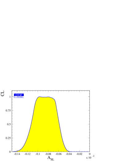
Figure 1: Confidence levels of $A_{\rm SL}$ in the Standard Model.

In Fig. 1 we show the Standard Model prediction for $A_{\rm SL}$, using the $R$fit approach in the CkmFitter package Hocker:2001xe , where theoretical errors are considered as allowed ranges Harrison:1998yr ; Hocker:2001xe . With the above input parameters, the range of $A_{\rm SL}$ values with greater than 10% CL is

$$-1.28\times 10^{-3}<A_{\rm SL}<-0.48\times 10^{-3}\,.$$ (18)

The range with greater than 32% CL (that would correspond to a “$1\sigma$ range” if the theoretical errors were negligible) is only slightly smaller, $-1.18\times 10^{-3}<A_{\rm SL}<-0.55\times 10^{-3}$. This indicates that the uncertainty in eq. (18) is dominated by theoretical errors, resulting in the plateau in Fig. 1 with a confidence level near unity. The uncertainty will decrease when the constraints on $\bar{\eta}$ improve, the NLO correction to $\Gamma_{12}$ is computed, and the $b$ quark mass is more precisely determined. We did not assign an error to the assumption of local quark-hadron duality which enters the OPE calculation of the nonleptonic $B$ decay rates determining $\Gamma_{12}$. We may gain confidence that the errors related to this are small if future lattice calculations can account for the $b$ hadron lifetimes and, especially, for the $B_{s}$ lifetime difference.

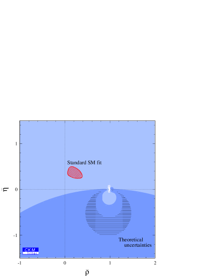
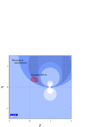
Figure 2: The constraint on the $\bar{\rho}-\bar{\eta}$ plane from the present data on $A_{\rm SL}$ in eq. (4) (left); and the constraint that would follow from a hypothetical value $A_{\rm SL}=(-1\pm 3)\times 10^{-3}$ (right). The central value of the latter was chosen to be consistent with the SM, and the error may be achievable by 2005. The dark-, medium-, and light-shaded regions have confidence levels above 90%, 32%, and 10%, respectively. The white regions contain points with at most 10% CL.

At leading order, corresponding to $A_{\rm SL}^{0}$ in eq. (5), a constraint $X_{-}<A_{\rm SL}<X_{+}$ with $X_{+}>0$ and $X_{-}<0$ excludes the interior of two circles, one with radius $R_{+}$ around the point $(\bar{\rho},\bar{\eta})=(1,-R_{+})$, and another with radius $R_{-}$ around the point $(\bar{\rho},\bar{\eta})=(1,R_{-})$. With the above central values of the input parameters, $R_{\pm}=\kappa/(2|X_{\pm}|)\simeq 6.7\times 10^{-4}/|X_{\pm}|$. If $X_{+}<0$ [$X_{-}>0$], then the corresponding excluded region is the outside of a circle of radius $R_{+}$ [$R_{-}$] around the point $(1,R_{+})$ [$(1,-R_{-})$]. Including the terms in $a_{\rm SL}^{z}$ distorts these circles by making them slightly larger for $\bar{\rho}<1$ than for $\bar{\rho}>1$, as shown in Fig. 2.

In Fig. 2, the left plot shows the constraint that the present data on $A_{\rm SL}$, eq. (4), provide on the $\bar{\rho}-\bar{\eta}$ plane. The right plot shows the constraint that would follow from a hypothetical future value $A_{\rm SL}=(-1\pm 3)\times 10^{-3}$. We chose the central value to be within the SM allowed range and the error to represent an experimental accuracy that may be achievable with 500 fb^-1 data expected by 2005 at the $B$ factories, using a simple statistical scaling of the BABAR result Aubert:2002mn , which is based on 20 fb^-1 data and is the most precise one in eq. (3). The dark shaded regions contain the points with confidence levels above 90%, and include the best fit points. The dark and medium shaded regions together contain the “one sigma” allowed regions with CL above 32%. The dark-, medium-, and light-shaded regions together contain all points with CL higher than 10%. Thus, the white regions have at most 10% CL. The small diagonally hatched areas show the SM allowed region (points with greater than 10% CL). The horizontally stripped regions contain the points with CL above 10% for a hypothetical “perfect” measurement of $A_{\rm SL}=+0.002$ (left plot) and $A_{\rm SL}=-0.001$ (right plot). These illustrate the significance of the present theoretical errors in interpreting the experimental results, and the importance of reducing them by determining $m_{b}$ and $z$ more precisely and especially by completing the NLO calculation of $\Gamma_{12}$.

One sees that within the next few years $A_{\rm SL}$ will not be a useful constraint on $(\bar{\rho},\bar{\eta})$ in the context of the Standard Model if the experimental result remains consistent with the SM prediction. However, as we discuss it next, it is a sensitive probe of new physics, and already provides interesting constraints on certain models.

III $A_{\rm SL}$ with New Physics

III.1 Analytical Expressions

We investigate $A_{\rm SL}$ in models of new physics Sanda:1997rh ; Randall:1998te ; Cahn:1999gx ; Barenboim:1999in with the following two features:

(i) The $3\times 3$ CKM matrix is unitary.

(ii) Tree level processes are dominated by the SM.

The second feature means that $\Gamma_{12}=\Gamma_{12}^{\rm SM}$, and the new physics effects modify only $M_{12}$. Then, quite generally, these effects can be parameterized by two new parameters, $\theta_{d}$ and $r_{d}$, defined through

$$M_{12}=r_{d}^{2}\,e^{2i\theta_{d}}M_{12}^{\rm SM}.$$ (19)

This modification involves well-known consequences for the mass difference between the neutral $B$ mesons,

$$\Delta m_{B}=r_{d}^{2}(\Delta m_{B})^{\rm SM},$$ (20)

and for the CP asymmetry in charmonium-containing $b\to c\bar{c}s$ decays, which is denoted throughout this paper by $a_{\psi K}$,

$$a_{\psi K}=\sin(2\beta+2\theta_{d}).$$ (21)

For the CP asymmetry in semileptonic decays, the modification from the Standard Model value depends on both $r_{d}^{2}$ and $2\theta_{d}$:

$$A_{\rm SL}=-\mbox{Re}\left({\Gamma_{12}\over M_{12}}\right)^{\rm SM}{\sin 2\theta_{d}\over r_{d}^{2}}+\mbox{Im}\left({\Gamma_{12}\over M_{12}}\right)^{\rm SM}{\cos 2\theta_{d}\over r_{d}^{2}}.$$ (22)

The first term has been previously investigated. Since ${\rm Re}({\Gamma_{12}/M_{12}})^{\rm SM}$ is larger than $A_{\rm SL}^{\rm SM}$ by a factor of order $m_{b}^{2}/m_{c}^{2}$, it could give an asymmetry that is an order of magnitude larger than the Standard Model prediction. This would happen if the new physics contribution to $M_{12}$ has a large new phase ($\sin 2\theta_{d}\not\ll 1$). The second term is suppressed by $m_{c}^{2}/m_{b}^{2}$ compared to the first one, however, one might expect it to be enhanced in the region $\sin 2\theta_{d}\approx 0$ and $r_{d}^{2}\ll 1$, corresponding to cancelling contributions to $\Delta m_{B}$ from the Standard Model and from new physics. However, we find that this term plays a numerically negligible role as long as the error of $A_{\rm SL}$ is much larger than the SM expectation.

Our purpose is to find the constraints on $r_{d}^{2}$ and $2\theta_{d}$ from the present measurements of $A_{\rm SL}$. We need therefore to evaluate $(\Gamma_{12}/M_{12})^{\rm SM}$. In ref. Dighe:2001gc one can find the $m_{c}^{2}/m_{b}^{2}$, $1/m_{b}$, penguin and NLO QCD corrections. Given the present experimental accuracy, it is sufficient for our purposes to include only corrections of order 10%, that is, ${\cal O}(z)$ and ${\cal O}(1/m_{b})$ corrections:

$$\left({\Gamma_{12}\over M_{12}}\right)^{\rm SM}= - {4\pi m_{b}^{2}\over 3m_{W}^{2}\bar{\eta}_{B}S_{0}(m_{t}^{2}/m_{W}^{2})}\,\Bigg{[}{5\over 8}(K_{2}-K_{1}){B_{S}^{\prime}\over B}+\left(K_{1}+{K_{2}\over 2}\right)$$ (23)

$$+ \left({K_{1}\over 2}-K_{2}\right){m_{B}^{2}-m_{b}^{2}\over m_{b}^{2}}{1\over B}-3z(K_{1}+K_{2}){1-\bar{\rho}-i\bar{\eta}\over(1-\bar{\rho})^{2}+\bar{\eta}^{2}}\Bigg{]}.$$

There are four parameters related to flavor violation that are relevant to our discussion here: the CKM parameters $\bar{\rho}$ and $\bar{\eta}$ and the new physics parameters of eq. (19) $r_{d}^{2}$ and $2\theta_{d}$. There are also four critical constraints: $|V_{ub}|$ from charmless semileptonic $B$ decays (these are tree level processes and therefore, by assumption, unaffected by the new physics), $\Delta m_{B}$ of eq. (20), $a_{\psi K}$ of eq. (21), and $A_{\rm SL}$ of eq. (22). In the next subsection we study the consistency of these four measurements and their combined constraints on the model parameters. Note that we cannot use the measured value of $\epsilon_{K}$ and the lower bound on $\Delta m_{B_{s}}$ since they may involve additional parameters.

III.2 Numerical Results

Fig. 3 shows the allowed range of $A_{\rm SL}$ for arbitrary $r_{d}$ and $\theta_{d}$ using the constraints from $|V_{ub}|$, $\Delta m_{B}$, and $a_{\psi K}$. To evaluate eq. (23), we used the $\overline{\rm MS}$ $b$ quark mass in the overall factor, as in sec. II.B. The black curve superimposed in Fig. 3 shows the confidence level corresponding to the measured value of $A_{\rm SL}$ in eq. (4). In the presence of new physics that can be parameterized by $r_{d}$ and $\theta_{d}$, the range of $A_{\rm SL}$ with greater than 10% CL is $-0.4\times 10^{-2}<A_{\rm SL}<3.9\times 10^{-2}$, whereas the measurement in eq. (4) implies $-2.1\times 10^{-2}<A_{\rm SL}<2.5\times 10^{-2}$ at the same CL. Clearly, the recent measurements of $A_{\rm SL}$ are sensitive enough to probe new physics, and already constrain the $r_{d}^{2}-2\theta_{d}$ parameter space.

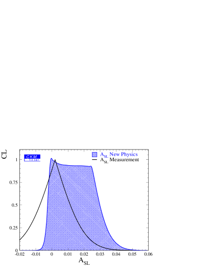
Figure 3: The filled area shows the confidence levels of $A_{\rm SL}$ for arbitrary $r_{d}$ and $\theta_{d}$ using the constraints from $|V_{ub}|$, $\Delta m_{B}$, and $a_{\psi K}$. The curve represents the measured value of $A_{\rm SL}$ in eq. (4), and indicates that some new physics models are being excluded.

It is interesting to note that if $A_{\rm SL}$ is negative, as in the SM, then new physics that can be parameterized by $r_{d}$ and $\theta_{d}$ can only enhance it by a factor of few. However, if new physics makes $A_{\rm SL}$ positive, then it can be enhanced by more than an order of magnitude. The reasons for this situation are explained below.

   

   

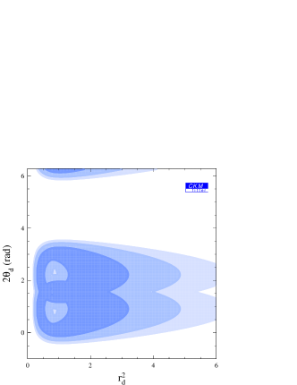
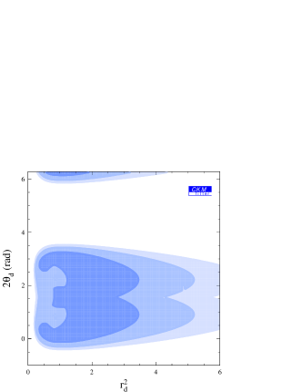
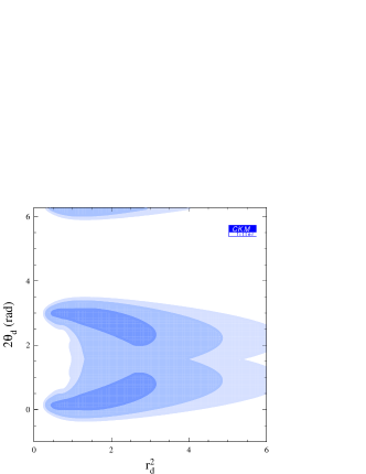
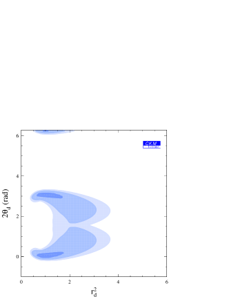
Figure 4: The top left plot shows the confidence levels of $r_{d}^{2}$ and $2\theta_{d}$ from the measurements of $|V_{ub}|$, $\Delta m_{B}$, and $a_{\psi K}$; the top right plot also includes $A_{\rm SL}$ as a constraint. The bottom left plot shows the confidence levels corresponding to a hypothetical future value $A_{\rm SL}=(-1\pm 3)\times 10^{-3}$, while the bottom right plot assumes in addition reduced errors in $|V_{ub}|$ (10%), $f_{B}$ (10 MeV) and $a_{\psi K}$ (0.04). The shadings mean the same as in Fig. 2.

The top left plot in Fig. 4 shows the confidence levels of $r_{d}^{2}$ and $2\theta_{d}$ from the measurements of $|V_{ub}|$, $\Delta m_{B}$, and $a_{\psi K}$. The ranges with greater than 10% CL are

$$0.2<r_{d}^{2}<6.4\,,\qquad-0.4<2\theta_{d}<3.6\,.$$ (24)

The errors are again dominated by theoretical ranges, except for the upper bound on $r_{d}^{2}$. Consequently, the ranges with greater than 32% CL, $0.2<r_{d}^{2}<5.2$ and $-0.3<2\theta_{d}<3.5$, only differ significantly from eq. (24) in $(r_{d}^{2})_{\rm max}$. This plot makes it clear why new physics can enhance much more a positive $A_{\rm SL}$ value than a negative one. First, since $a_{\psi K}>0$ is firmly established, the maximal allowed magnitude of $\sin 2\theta_{d}$ is larger for positive values than it is for negative ones Eyal:1999ii . Second, the correlations between the three constraints are such that while maximal positive $\sin 2\theta_{d}$ and minimal $r_{d}^{2}$ are allowed simultaneously, this is not the case for negative $\sin 2\theta_{d}$. The top right plot shows the present constraints on the $r_{d}^{2}-2\theta_{d}$ plane, including also the measurement of $A_{\rm SL}$. The measurement of $A_{\rm SL}$ has an noticeable impact: in particular, the lowest values of $r_{d}^{2}$ (around 0.2) are now disfavored, and almost the entire $r_{d}^{2}\lesssim 0.5$ region is no longer among the best-fit points. The bottom left plot show the constraints that would follow from a hypothetical future value, $A_{\rm SL}=(-1\pm 3)\times 10^{-3}$. Such a measurement would be able to exclude a large part of the $r_{d}^{2}<1$ parameter space (i.e., cancelling contributions to $\Delta m_{B}$ from the SM and new physics), except if $2\theta_{d}$ were near $0$ or $\pi$. This plot is rather insensitive to the expected reduction of the error of $a_{\psi K}$ by itself, while additional improvements in $|V_{ub}|$ and $\Delta m_{B}$ will make a significant difference. This is shown in the bottom right plot, where reduced errors about the present central values in $|V_{ub}|$ (10%), $f_{B}$ (10 MeV) and $a_{\psi K}$ (0.04) are also assumed.

III.3 The $B_{s}$ system

Similar analyses will become possible in the future for the $B_{s}$ system. Within the SM, the semileptonic asymmetry in $B_{s}$ decays is suppressed even more strongly than the asymmetry in $B_{d}$ decays. (For the sake of clarity, we now call the respective asymmetries $A_{\rm SL}^{s}$ and $A_{\rm SL}^{d}$.) While the $m_{c}^{2}/m_{t}^{2}$ suppression factor in eq. (6) is common to both, the CKM dependence is different. For $A_{\rm SL}^{d}$ it is given by eq. (7), which is a factor of order unity. In contrast, for $A_{\rm SL}^{s}$ it is given by $\mbox{Im}\left({V_{cb}V_{cs}^{*}\over V_{tb}V_{ts}^{*}}\right)\approx-\frac{1}{2}\sin 2\beta_{s}$. In Fig. 5 we give the CL for $\sin 2\beta_{s}$ within the SM. We learn that the range of $\sin 2\beta_{s}$ with greater than 10% CL is

$$0.026<\sin 2\beta_{s}<0.048\,,$$ (25)

Consequently, $A_{\rm SL}^{s}$ is unobservably small in the SM.

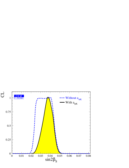
Figure 5: Confidence levels of $\sin 2\beta_{s}$ in the Standard Model.

Defining $M_{12}^{s}\equiv r_{s}^{2}e^{2i\theta_{s}}(M_{12}^{s})^{\rm SM}$, the present lower bound from the LEP/SLD/CDF combined amplitude fit (corresponding to $\Delta m_{B_{s}}>15.0\,\mbox{ps}^{-1}$) implies

$$r_{s}^{2}>0.6\,,$$ (26)

whereas there is no constraint on $\theta_{s}$ yet. These parameters can be determined in the future in the following ways: (i) A measurement of $\Delta m_{B_{s}}$ will constrain $r_{s}^{2}$. (ii) A measurement of the CP asymmetry in $B_{s}\to\psi\phi$ or $\psi\eta^{(\prime)}$ will constrain $\sin 2(\beta_{s}+\theta_{s})$. If the asymmetry is much larger than the SM range, it practically determines $\sin 2\theta_{s}$. (iii) A measurement of $A_{\rm SL}^{s}$ will be proportional to $\sin 2\theta_{s}/r_{s}^{2}$ and will give a consistency check on the interpretation of the previous two measurements. The values of the four parameters $r_{d}^{2}$, $2\theta_{d}$, $r_{s}^{2}$ and $2\theta_{s}$ provide an excellent probe of the flavor and CP structure of new physics.

IV $A_{\rm SL}$ with Minimal Flavor Violation

IV.1 Analytical Expressions

Minimal flavor violation (MFV) is the name given to a class of new physics models that do not have any new operators beyond those present in the Standard Model and in which all flavor changing transitions are governed by the CKM matrix with no new phases beyond the CKM phase Ciuchini:1998xy ; Ali:1999we ; Buras:2000dm ; Buras:2000xq ; Buras:2001af ; Buras:2001pn ; Bergmann:2001pm . Examples include the constrained minimal supersymmetric Standard Model and the two Higgs doublet models of types I and II. In these models, the SM predictions for some flavor changing processes remain unchanged, while other are modified but in a correlated way. The new physics contributions that are relevant to our discussion depend on a single new parameter, $F_{tt}$, that is real but could have either sign. These models can be viewed as special cases of sec. III — the correspondence is $r_{d}^{2}=|F_{tt}|/S_{0}$ and $2\theta_{d}=0\ (\pi)$ for $F_{tt}>0\ (<0)$ — with the additional constraints, (ii) and (v) below:

(i) Semileptonic $B$ decays depend on $|V_{ub}/V_{cb}|$ in the same way as in the Standard Model.

(ii) The ratio $\Delta m_{B}/\Delta m_{B_{s}}$ depends on $|V_{td}/V_{ts}|$ in the same way as in the Standard Model.

(iii) The CP asymmetry $a_{\psi K}$ depends on the sign of $F_{tt}$ Buras:2001af :

$$a_{\psi K}={\rm sign}(F_{tt})\sin 2\beta\,.$$ (27)

(iv) The mass difference $\Delta m_{B}$ depends on $|F_{tt}|$:

$$\Delta m_{B}=(\Delta m_{B})^{\rm SM}\,{|F_{tt}|\over S_{0}}\,.$$ (28)

(The QCD correction in MFV models may differ from $\eta_{B}$, but the modification is the same for $\Delta m_{B_{d,s}}$ and for the top contribution to $\epsilon_{K}$, so it can be absorbed in $F_{tt}$ Buras:2000xq .)

(v) The Standard Model contribution to $\epsilon_{K}$ that is proportional to Im[$(V_{ts}V_{td}^{*})^{2}$] is multiplied by $F_{tt}$ while the other contributions remain unchanged:

$$\epsilon_{K}=\epsilon_{tt}^{\rm SM}F_{tt}+\epsilon_{ct}^{\rm SM}+\epsilon_{cc}^{\rm SM}.$$ (29)

The constraints on $\bar{\rho}$, $\bar{\eta}$ and $F_{tt}$ from these processes have been analyzed in a number of papers (see, for example, Buras:2000dm ; Bergmann:2001pm ). In this section we present the MFV predictions for $A_{\rm SL}$.

The dependence of $A_{\rm SL}$ on new contributions is simple. Since for the $B^{0}-\overline{B}{}^{0}$ mixing amplitude one has $M_{12}=(M_{12})^{\rm SM}F_{tt}/S_{0}$, while $\Gamma_{12}$ is not modified, we obtain:

$$A_{\rm SL}^{\rm MFV}=A_{\rm SL}^{\rm SM}\,{S_{0}\over F_{tt}}\,.$$ (30)

Thus the size of $A_{\rm SL}$ may be different from the Standard Model.

As concerns the sign of $A_{\rm SL}$, one might naively think that it could be opposite to the Standard Model prediction, since ${\rm sign}(A_{\rm SL}^{\rm MFV})\propto{\rm sign}(F_{tt})$. However, this is not the case, because ${\rm sign}(A_{\rm SL}^{\rm SM})=-{\rm sign}(\bar{\eta})$, and so

$${\rm sign}(A_{\rm SL}^{\rm MFV})=-{\rm sign}(\bar{\eta}F_{tt}).$$ (31)

The product $\bar{\eta}F_{tt}$ (in combination with the upper bound on $|V_{ub}/V_{cb}|$ which implies $\bar{\rho}<1$) determines, however, also the sign of $a_{\psi K}$:

$${\rm sign}(a_{\psi K}^{\rm MFV})={\rm sign}(\bar{\eta}F_{tt}),$$ (32)

and is therefore experimentally determined to be positive. We conclude that there can be no sign difference between the SM and MFV predictions for $A_{\rm SL}$. In other words, if $A_{\rm SL}$ is experimentally found to be positive, both the Standard Model and the MFV models will be excluded.

IV.2 Numerical Results

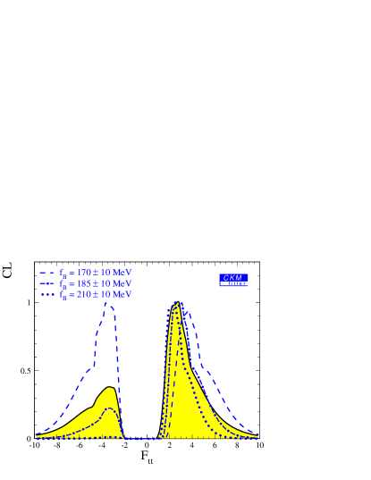
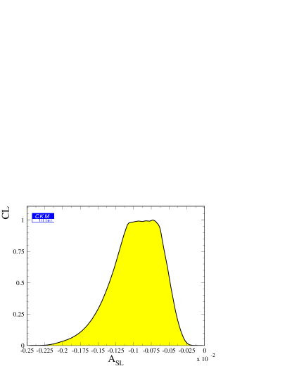
Figure 6: Left: Confidence levels of $F_{tt}$. The shaded region corresponds to our ranges for the input parameters (in particular, $f_{B}=200\pm 30\,$MeV). The other curves show the sensitivity to $f_{B}$: $f_{B}=170\pm 10\,$MeV (dashed), $f_{B}=190\pm 10\,$MeV (dash-dotted), and $f_{B}=210\pm 10\,$MeV (dotted). In this last case the $F_{tt}<0$ solution is excluded. Right: Confidence levels of $A_{\rm SL}$ in MFV models.

The shaded region in the left plot in Fig. 6 shows the confidence levels of $F_{tt}$ obtained from the above constraints. The range of $F_{tt}$ with greater than 10% CL is

$$-7.3<F_{tt}<-2.4\qquad\mbox{and}\qquad 1.2<F_{tt}<7.3\,.$$ (33)

The range corresponding to greater than 32% CL is $-4.3<F_{tt}<-2.7$ and $1.4<F_{tt}<5.1$. This implies, using eq. (30) and $S_{0}(m_{t}^{2}/m_{W}^{2})\simeq 2.4$, that the magnitude of $A_{\rm SL}$ can hardly be enhanced compared to the SM, as it is shown in the right plot in Fig. 6. The range of $A_{\rm SL}$ values with greater than 10% CL in MFV models is

$$-1.77\times 10^{-3}<A_{\rm SL}<-0.33\times 10^{-3}\,,$$ (34)

while the greater than 32% CL range is $-1.48\times 10^{-3}<A_{\rm SL}<-0.43\times 10^{-3}$. Thus, a measurement of $A_{\rm SL}$ significantly above the SM prediction would exclude both the Standard Model, and models with minimal flavor violation.

The existence of the $F_{tt}<0$ solution is sensitive to the value of $f_{B}$ (this was first pointed out in Ref. Buras:2001af ). This is shown by the curves superimposed on the left plot in Fig. 6, corresponding to $f_{B}=170\pm 10\,$MeV (dashed), $f_{B}=190\pm 10\,$MeV (dash-dotted), and $f_{B}=210\pm 10\,$MeV (dotted). If future unquenched lattice calculations obtain $f_{B}$ above $200\,$MeV with small error, then the confidence level of the $F_{tt}<0$ solution is reduced, and this solution practically disappears if $f_{B}=210\pm 10\,$MeV or larger. Note also that if the value of $f_{B}$ decreases then the CL of the $F_{tt}<0$ solution increases, while that of the $F_{tt}>0$ solution is reduced. For example, for $f_{B}=170\pm 10\,$MeV, both solutions have about equal CL, and if $f_{B}=160\pm 10\,$MeV then the CL of the $F_{tt}>0$ solution is hardly above 50%.

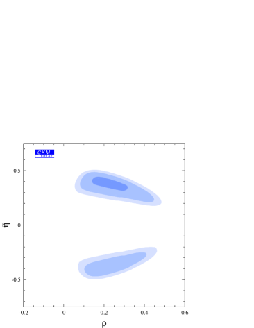
Figure 7: The allowed $\bar{\rho}-\bar{\eta}$ range in MFV models. The shadings mean the same as in Fig. 2.

Fig. 7 shows the allowed range of $\bar{\rho}$ and $\bar{\eta}$ in MFV models. In agreement with Fig. 6, it can be seen that the $\bar{\eta}<0$ solution is less favored than the allowed $\bar{\eta}>0$ region.

V Conclusions

We investigate $A_{\rm SL}$, the CP asymmetry in semileptonic $B$ decays, in three theoretical frameworks.

Within the Standard Model, we improve previous predictions by including corrections of order $m_{c}^{2}/m_{b}^{2}$ and $\Lambda_{\rm QCD}/m_{b}$ [see eq. (17)]. This leaves the NLO corrections, of order $\alpha_{s}$, as the largest source of uncertainty. Our improved calculation gives that the allowed range of $A_{\rm SL}$, corresponding to greater than 10% CL, is: $-1.3\times 10^{-3}<A_{\rm SL}<-0.5\times 10^{-3}$. The smallness of the asymmetry means that even with improved statistics in the $B$ factories, no useful constraints on the CKM matrix will arise within the next few years.

Within models of minimal flavor violation, a mild enhancement of the asymmetry is possible, $-1.8\times 10^{-3}<A_{\rm SL}<-0.3\times 10^{-3}$. This is again too small to be observed in the near future. Conversely, if the asymmetry is measured with a value that is much larger than the SM range, MFV will be excluded. Moreover, within MFV models, the SM relation, sign($A_{\rm SL})=-$sign($a_{\psi K})$, is maintained; a measurement of a positive $A_{\rm SL}$ would therefore exclude both the SM and MFV.

The recent measurements of $A_{\rm SL}$ do already have meaningful consequences in probing less constrained extensions of the SM, where there are new sources of flavor and CP violation. In particular, in models where the new effects can be neglected in tree-level decays but are significant in flavor changing neutral current processes, the four observables — $|V_{ub}|$ from charmless semileptonic $B$ decay rates, $\Delta m_{B}$, $a_{\psi K}$ and $A_{\rm SL}$ — depend on four parameters: the two CKM parameters $\bar{\rho}$ and $\bar{\eta}$ and the two new parameters $r_{d}^{2}$ and $2\theta_{d}$ [see eq. (19)]. In this framework, $A_{\rm SL}$ makes an impact in constraining the allowed range in the $r_{d}^{2}-2\theta_{d}$ plane, especially in the region of small $r_{d}^{2}$ and large $\sin 2\theta_{d}$. In this region, there is strong cancellation between the SM and the new contributions to $B^{0}-\overline{B}{}^{0}$ mixing, which minimizes the magnitude of the dispersive part and maximizes the relative phase between the dispersive and absorptive parts. Under these circumstances, $A_{\rm SL}$ is much enhanced and opposite in sign to the Standard Model prediction. The recent experimental results disfavor such a possibility (see Fig. 3).

We conclude that improved bounds on $A_{\rm SL}$ will further constrain new physics contributions to $B^{0}-\overline{B}{}^{0}$ mixing. If a sizable value of $A_{\rm SL}$ is measured in the near future, not only the Standard Model but also its extensions with minimal flavor violation will be excluded.