Constraints on Models for Proton-Proton Scattering from Multi-strange Baryon Data

Abstract

The recent data on pp collisions at 158 GeV provide severe constraints on string models: These measurements allow for the first time to determine how color strings are formed in ultrarelativistic proton-proton collisions.

1 Introduction

Recently, the NA49 collaboration has published [1] the rapidity spectra of p, $\Lambda$, $\Xi$ as well as the corresponding antibaryons in pp interactions at 158 GeV. These measurements provide new insight into the string formation process. In the string picture, high energy proton-proton collisions create “excitations” in form of strings, being one dimensional objects which decay into hadrons according to longitudinal phase space. This framework is well confirmed in low energy electron-positron annihilation [2] where the virtual photon decays into a quark-antiquark string which breaks up into mesons($M$), baryons($B$) and antibaryons($\overline{B}$). An example of a $\mathrm{q}-\overline{\mathrm{q}}$ string fragmenting into hadrons is shown in Fig.1. Proton-proton collisions are more complicated due to the fact that even at 158 GeV proton-proton collisions are governed by soft physics, thus pQCD calculations can not be applied. And the mechanism of string formation is not clear, as will be discussed in the following.

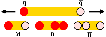
Figure 1: $\mathrm{e}^{+}\mathrm{e}^{-}\rightarrow\gamma^{*}\rightarrow\mathrm{q}\overline{\mathrm{q}}$. The $\mathrm{q}-\overline{\mathrm{q}}$ string fragments into hadrons.

One may distinguish two classes of string models:

• Longitudinal excitation (LE) models: UrQMD [3], HIJING [4], PYTHIA [5], FRITIOF [6];

• Color exchange (CE) models: DPM [7], VENUS [2], QGS [8].

  

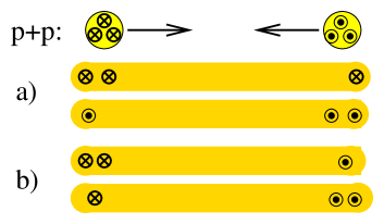
  Figure 2: Two string formation mechanisms for pp collisions are presented: a) longitudinal excitation (LE). b) color exchange (CE).

In the LE case the two colliding protons excite each other via a large transfer of momentum between projectile and target, Fig.2a. In contrast, the CE picture considers a color exchange between the incoming protons, leaving behind two octet states. Thus, a diquark from the projectile and a quark from the target, and vice versa, form color singlets. These are identified with strings, c.f. Fig.2b. The color exchange is a soft process. The transfer of momentum is negligible. The final result, two quark-diquark strings with valence quarks being their ends, however, is quite similar.

How are baryons and antibaryons produced? The easiest way to obtain baryons is to break the strings via quark-antiquark pair production close to the valence diquark. Since the ingoing proton was composed of light quarks(qqq), the resulting baryon is of qqq or qqs type. Thus nucleons, $\Lambda$s or $\Sigma$s are formed. Since these baryons are produced at the string ends, they occur mainly close to the projectile rapidity or target rapidity (leading baryons).

Multi-strange baryons which consist of two or three strange quarks are produced near the quark end or the middle of the strings, via ss-${\overline{\mathrm{s}}}{\overline{\mathrm{s}}}$ production. Therefore the distributions of multi-strange baryons are peaked around central rapidity and the corresponding yields of multi-strange baryons and their antiparticles should be comparable. A closer look reveals an interesting phenomenon: Theoretically one finds the ratio of yields [9]:

$$\overline{\Xi}^{+}/\Xi^{-}=0.8\sim 1.2\,.$$

Experimentally, however, $\overline{\Xi}^{+}$s are less frequent than expected. The ratio at midrapidity is [1]

$$\overline{\Xi}^{+}/\Xi^{-}=0.44\pm 0.08.$$

The situation for $\Omega$s is even more extreme: from string models one gets [9]

$$\overline{\Omega}^{+}/\Omega^{-}=1.6\sim 1.9$$

at midrapidity. From extrapolating $\Lambda$ and $\Xi$ results (and from preliminary NA49 data) we expect [1]

$$\overline{\Omega}^{+}/\Omega^{-}=0.5\sim 0.8\,.$$

This is a generic situation; It is impossible to get the $\overline{\Omega}^{+}/\Omega^{-}$ ratio smaller than unity from those two types of string models. As addressed in [9], this is due to the fact that the strings have a light quark (but not a strange quark) at the end, which disfavours multi-strange baryon production, and does not allow for $\Omega$ production in the fragmentation region.

2 Problems with the String Model Approach

So is there something fundamentally wrong with string models? To answer this question let us consider somewhat more in detail how string models are realized. One may present the particle production from strings via chains of quark lines [7] as shown in fig. 3.

a)             b) 

Figure 3: Two chains of quark lines (b) representing a pair of strings (a)

It turns out that the two string picture is not enough to explain for example the large multiplicity fluctuations in proton-proton scattering at collider energies: more strings are needed, one adds therefore one or more pairs of quark-antiquark strings, as shown in fig. 4.

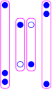
a)             b) 

Figure 4: Two pairs of strings (a) and the corresponding chains (b)

The variables $x_{i}$ refer to the longitudinal momentum fractions given to the string ends. Energy-momentum conservation implies $\sum x_{i}=1.$

What is the probabilities for different string numbers? Here, Gribov-Regge theory comes at help, which tells us that the probability for a configuration with $n$ elementary interactions is given as

$$\mathrm{Prob}(n\,\mathrm{interactions})=\frac{\chi^{n}}{n!}\exp(-\chi),$$

where $\chi$ is a function of energy and impact parameter, see fig. 5.

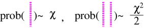
Figure 5: Probabilities for configurations with one and two elementary interactions (Pomerons), represented as dashed lines.

Here, a dashed vertical line represents an elementary interaction (referred to as Pomeron).

Now one identifies the elementary interactions (Pomerons) from Gribov-Regge theory with the pairs of strings (chains) in the string model, and one uses the above-mentioned probability for $n$ Pomerons to be the probability for configurations with $n$ string pairs. Unfortunately this is not at all consistent, for two reasons:

1. Whereas in the string picture the first and the subsequent pairs are of different nature, in the Gribov-Regge model all the Pomerons are identical.

2. Whereas in the string (chain) model the energy is properly shared among the strings, in the Grivov-Regge approach does not consider energy sharing at all (the $\chi$ is a function of the total energy only)

These problems have to be solved in order to make reliable predictions.

3 Basic Ideas of Parton-Based Gribov-Regge Theory

We consider a new approach called Parton-Based Gribov-Regge theory to solve the above-mentioned problems. Here we still use the language of Pomerons as in Gribov-Regge theory to calculate probabilities of collision configurations and the language of strings to treat particle production. Multiple interactions happen in parallel. An elementary interaction is referred to as Pomeron. The spectators of each proton form a remnant, see Fig. 6. A Pomeron is finally identified with two strings, see Fig.7. But we treat both aspects in a consistent fashion: In both cases energy sharing is considered in a rigorous way[10], and in both cases all Pomerons are identical. This is the new feature of our approach, and the second point is exactly the solution to multistrange baryon problem mentioned above. In the following we discuss how to realize the collision configuration and particle production, respectively.

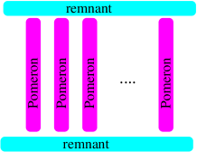
Figure 6: Multiple elementary interactions (Pomerons) in NEXUS.

Figure 7: Multiple elementary interaction (Pomerons) in NEXUS (a). An elementary interaction is identified with a pair of strings.

4 Collision Configuration

Gribov-Regge theory is applied in NEXUS to calculate collision configurations. This calculation is performed under the condition that energy sharing is considered rigorously. Once a collision configuration is determined, not only the number of Pomerons but also the energy sharing among Pomerons is fixed. This is different from other string models. In the following we discuss how to realize it in a qualitative fashion.

4.1 Reminder: some Elementary Quantum Mechanics

Let us introduce some conventions. We denote elastic two body scattering amplitudes as $T_{2\rightarrow 2}$ and inelastic amplitudes corresponding to the production of some final state $X$ as $T_{2\rightarrow X}$ (see fig.8 ).

      

Figure 8: An elastic scattering amplitude $T_{2\rightarrow 2}$ (left) and an inelastic amplitude $T_{2\rightarrow X}$ (right).

As a direct consequence of unitarity on has $2\,\mathrm{Im}T_{2\rightarrow 2}=\sum_{x}$$(T_{2\rightarrow X})$$(T_{2\rightarrow X})^{*}$. The right hand side of this equation may be literally presented as a “cut diagram”, where the diagram on one side of the cut is $(T_{2\rightarrow X})$ and on the other side $(T_{2\rightarrow X})^{*}$, as shown in fig.9 .

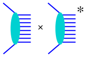
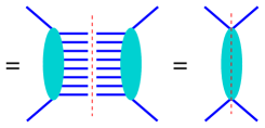
Figure 9: The expression $\sum_{X}(T_{2\rightarrow X})$$(T_{2\rightarrow X})^{*}$which may be represented as a “cut diagram”.

So the term “cut diagram” means nothing but the square of an inelastic amplitude, summed over all final states, which is equal to twice the imaginary part of the elastic amplitude. Based on these considerations, we introduce simple graphical symbols, which will be very convenient when discussing multiple scattering, shown in fig. 10: a vertical solid line represents an elastic amplitude (multiplied by $i$, for convenience), and a vertical dashed line represents the mathematical expression related to the above-mentioned cut diagram (divided by $2s$, for convenience).

,  

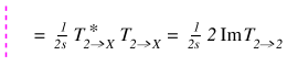
Figure 10: Conventions.

4.2 Elementary Interactions

Elementary nucleon-nucleon scattering can be considered as a straightforward generalization of photon-nucleon scattering: one has a hard parton-parton scattering in the middle, and parton evolutions in both directions toward the nucleons. We have a hard contribution $T_{\mathrm{hard}}$ when the the first partons on both sides are valence quarks, a semi-hard contribution $T_{\mathrm{semi}}$ when at least on one side there is a sea quark (being emitted from a soft Pomeron), with a perturbative process happening in the middle of Pomeron, and finally we have a soft contribution when no perturbative process happens at all (see fig. 11). The total elementary elastic amplitude $T_{2\rightarrow 2}$ is the sum of all contributions.

Figure 11: The elastic amplitude $T_{2\rightarrow 2}$.

The cut-off of virtuality between perturbative and non-perturbative processes, $Q_{0}^{2}$, is independent of the beam energy. The perturbative part of Pomeron is strictly based on the standard DGLAP evolution with ordered parton virtualities in the ladder diagram and the nonperturbative part is based on Reggeon parameterization. The semihard Pomeron is a convolution of hard and soft. The total elementary elastic amplitude $T_{2\rightarrow 2}$ is the sum of all these terms. Thus we have a smooth transition from soft to hard physics: at low energies the soft contribution dominates, at high energies the hard and semi-hard ones, at intermediate energies (that is where experiments are performed presently) all contributions are important.

The multiple scattering theory will be based on these elementary interactions, the corresponding elastic amplitude $T_{2\rightarrow 2}$ and the corresponding cut diagram, both being represented graphically by a solid and a dashed vertical line. We also refer to the solid line as Pomeron, to the dashed line as cut Pomeron.

4.3 Multiple Scattering

We first consider inelastic proton-proton scattering, see fig. 12. We imagine an arbitrary number of elementary interactions to happen in parallel, where an interaction may be elastic or inelastic. The inelastic amplitude is the sum of all such contributions with at least one inelastic elementary interaction involved.

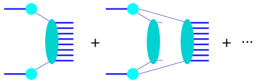
Figure 12: Inelastic scattering in pp.

To calculate cross sections, we need to square the amplitude, which leads to many interference terms, as the one shown in fig. 13(a), which represents interference between the first and the second diagram of fig. 12. Using the above notations, we may represent the left part of the diagram as a cut diagram, conveniently plotted as a dashed line, see fig. 13(b). The amplitude squared is now the sum over many such terms represented by solid and dashed lines.

(a)  (b)

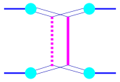
Figure 13: Inelastic scattering in pp. a) An interference term of cross section, b) Represented with our simplified notations.

When squaring an amplitude being a sum of many terms, not all of the terms interfere – only those which correspond to the same final state. For example, a single inelastic interaction does not interfere with a double inelastic interaction, whereas all the contributions with exactly one inelastic interaction interfere. So considering a squared amplitude, one may group terms together representing the same final state. In our pictorial language, this means that all diagrams with one dashed line, representing the same final state, may be considered to form a class, characterized by $m=1$ – one dashed line ( one cut Pomeron) – and the light cone momenta $x^{+}$ and $x^{-}$ attached to the dashed line (defining energy and momentum of the Pomeron). In fig. 14, we show several diagrams belonging to this class, in fig. 15, we show the diagrams belonging to the class of two inelastic interactions, characterized by $m=2$ and four light-cone momenta $x_{1}^{+}$, $x_{1}^{-}$, $x_{2}^{+}$, $x_{2}^{-}$.

   

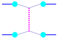
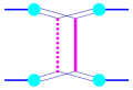
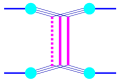
Figure 14: Class of terms corresponding to one inelastic interaction.

   

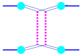
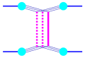
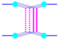
Figure 15: Class of terms corresponding to two inelastic interactions.

Generalizing these considerations, we may group all contributions with $m$ inelastic interactions ($m$ dashed lines = $m$ cut Pomerons) into a class characterized by the variable

$$K=\{m,x_{1}^{+},x_{1}^{-},\cdots,x_{m}^{+},x_{m}^{-}\}.$$

We then sum all the terms in a class $K$,

$$\Omega(K)=\sum\{\mathrm{all}\,\mathrm{terms}\,\mathrm{in}\,\mathrm{class}\,K\}.$$

The inelastic cross section is then simply a sum over classes,

$$\sigma_{\mathrm{inel}}(s)=\sum_{K\neq 0}\int d^{2}b\,\Omega(K).$$

$\Omega$ depends implicitly on the energy squared $s$ and the impact parameter $b$. The individual terms $\int d^{2}b\,\Omega(K)$, represent partial cross sections, since they represent distinct final states. They are referred to as topological cross sections. One can prove

$$\sum_{K}\Omega(K)=1,$$

which is a very important result justifying our interpretation of $\Omega(K)$ to be a probability distribution for the configurations $K$. This provides also the basis for applying Monte Carlo techniques.

The function $\Omega$ is the basis of all applications of this formalism. It is the foundation not only for calculating (topological) cross sections, but also for particle production, thus providing a consistent formalism for all aspects of a nuclear collision.

5 Particle Production

Here we discuss how to produce hadrons with any given collision configuration determined according to the above section. As we discussed above, each cut Pomeron is identified as a pair of strings. Similar to other string models, a Lorentz invariant string fragmentation procedure provides a transformation from strings to final-state hadrons in NEXUS. However the string formation mechanism in NEXUS is very different from others because Pomerons are treated identically for calculating particle production.

5.1 Hard Pomerons

As discussed above, each elementary interaction has hard, soft and semihard contribution. So each Pomeron has certain probabilities to be of type soft, hard and semihard. Once a collision configuration is determined according to the above section, the number of each type of Pomerons is fixed. To give a proper description of deep inelastic scattering data, hard and some of semihard Pomerons are connected to the valance quarks of the hadron. In order to conserve the initial hadron baryon content and to keep the simple factorized structure with the leading logarithmic approximation of quantum Chromodynamics, we associate a “quasi-spectator” antiquark (of the same flavour) to each valence quark interaction. So a hard Pomeron is a two-layer ladder diagram where one of them is hard with ordered virtualities and the other is soft. The hard ladder diagram gives a kinky string (each string segment has a constant velocity and finally is identified with those emitted perturbative partons). The fraction of hard Pomerons in total Pomerons is very subdominant in average proton-proton collisions. At SPS energies hard and semihard Pomerons do not contribute at all, and even at collider energies the Pomerons connected to valence quarks are rare. Therefore, even though all types of Pomerons are included in the Monte Carlo, their contribution can be ignored in the following discussion.

5.2 Soft Pomerons

How to form strings from soft Pomerons? No matter whether single-Pomeron exchange or multiple-Pomeron exchange happens in a proton-proton scattering, all Pomerons are treated identically. Because of this, it is a natural idea to take quarks and antiquarks from the sea as string ends, because an arbitrary number of Pomerons may be involved, and valence quarks are not always available to be string ends due to their limited amount. This point is different from the above-mentioned string models, where all the string ends are valence quarks. Letting all the valence quarks stay in remnants, thus, string ends from cut Pomerons have complete flavour symmetry and produce particles and antiparticles in equal amounts. In the old version of NEXUS used in [9], a sea quark and an antiquark of the same flavour have been taken from the sea as string ends to keep flavour conservation. In the new version, NEXUS 3.0, the flavours of the string ends are independent. In order to compensate the flavour, whenever a quark or an antiquark is taken from the sea as a string end, a corresponding antiparticle from the sea is put in the remnant nearby.

5.3 Remnant

Remnants are a new object, compared to other string models. The partonic content of a remnant is very clear: three valence quarks and the compensated partons. From this partonic structure one can estimate that its mass is of the order of proton mass. The 4-momentum of a remnant is that of an initial proton minus those being taken away by participant partons. So the 4-momenta of projectile remnant and target remnant are fixed once the collision configuration is given. The remnant mass can be calculated according to its 4-momentum and the on-shell condition, however this value of mass is not reliable. During the configuration calculation one distributes energy of order 100 GeV to Pomerons and remnants where a proton mass is negligible. We justify the remnant mass with a distribution $P(m^{2})\propto(m^{2})^{-\alpha}$, $m^{2}\in(m_{\mathrm{min}}^{2},\,x^{+}s)$, where $s$ is the squared energy at center mass system, $m_{\mathrm{min}}$ is the minimum mass of hadrons to be made from the remnant’s quarks and antiquarks, and $x^{+}$ is the light-cone momentum fraction of the remnant which is determined in the collision configuration. Through fitting the data we determine the parameter $\alpha=1.5$. Remnants decay into hadrons according to n-body phase space[11].

5.4 Leading Order Discussion

The configuration of leading order has only one cut Pomeron. The most simple and most frequent collision configuration has two remnants and only one cut Pomeron represented by two $\mathrm{q}-\overline{\mathrm{q}}$ strings as in Fig.16a. Besides the three valence quarks, each remnant has additionally a quarks and an antiquark to compensate the flavour.

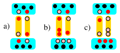
Figure 16: a) The most simple and frequent collision configuration has two remnants and only one cut Pomeron represented by two $\mathrm{q}-\overline{\mathrm{q}}$ strings. b) One of the $\overline{\mathrm{q}}$ string-ends can be replaced by a $\mathrm{qq}$ string-end. c) With the same probability, one of the $\mathrm{q}$ string-ends can be replaced by a $\overline{\mathrm{q}}\overline{\mathrm{q}}$ string-end.

The leg of a cut Pomeron may be of qqq type with small probability $P_{\mathrm{qq}}$, which means the corresponding string ends are a diquark and a quark. In this way we get quark-diquark (q-qq) strings from cut Pomerons. The qqq Pomeron leg has to be compensated by the three corresponding antiquarks in the remnant, as in Fig.16b. The (3q3$\overline{\mathrm{q}}$) remnant may decay into three mesons (3M) or a baryon and an anti-baryon (B+$\overline{\mathrm{B}}$). Since the 3M mode is favored by phase space, we neglect B+$\overline{\mathrm{B}}$ production here.

For symmetry reasons, the leg of a cut Pomeron is of $\overline{\mathrm{q}}\overline{\mathrm{q}}\overline{\mathrm{q}}$ type with the same probability $P_{\mathrm{qq}}$. This yields a $\overline{\mathrm{q}}-\overline{\mathrm{q}}\overline{\mathrm{q}}$ string and a (6q) remnant, as shown in Fig.16c. The (6q) remnant decays into two baryons. Since q-qq strings and $\overline{\mathrm{q}}-\overline{\mathrm{q}}\overline{\mathrm{q}}$ strings have the same probability to appear from cut Pomerons, baryons and antibaryons are produced equally. However, from remnant decay, baryon production is favored due to the initial valence quarks.

6 Results

Here, we will concentrate on baryon-antibaryon production, because there we obtain strikingly different results compared to other models. However, we carefully checked as well mesons – essentially pion and kaon rapidity and transverse momentum spectra, where the results are quite close to what we obtained earlier with NEXUS 2 or VENUS.

Fig.17 depicts the rapidity spectra of baryons and antibaryons from NEXUS 3.0 with $P_{\mathrm{qq}}=0.02$ (solid lines). As a comparison, we also show the preliminary data from the NA49 experiment [1] (points). The contributions of projectile remnants (dashed lines), target remnants (dotted lines) and cut Pomerons (dashed dotted lines) to particle production are also shown respectively in Fig.17. Fig.17 demonstrates that NEXUS 3.0 describes reasonably the rapidity spectra of baryons and antibaryons in pp collision at 158 GeV.

We also provide the particle yields at midrapidity, $y\in(y_{\mathrm{cm}}-0.5\,,\,y_{\mathrm{cm}}+0.5)$, from NEXUS 3.0, Pythia 6.2 and compare them to data in table 1.

yield	NEXUS 3.0	Pythia 6.2	NA49 data
p	9.12$\times$10-2	4.85$\times$10-2	9.28$\times$10-2
$\overline{\mathrm{p}}$	2.00$\times$10-2	1.64$\times$10-2	2.05$\times$10-2
$\Lambda$	1.61$\times$10-2	7.53$\times$10-3	1.79$\times$10-2
$\overline{\Lambda}$	5.85$\times$10-3	4.02$\times$10-3	5.57$\times$10-3
$\Xi^{-}$	8.08$\times$10-4	2.53$\times$10-4	7.08$\times$10-4
$\overline{\Xi}^{+}$	4.71$\times$10-4	2.20$\times$10-4	3.12$\times$10-4
$\Omega^{-}$	2.79$\times$10-5	2.33$\times$10-6	–
$\overline{\Omega}^{+}$	2.16$\times$10-5	2.94$\times$10-6	–

Table 1: Particle yields at midrapidity in pp collisions at 158 GeV.

From NEXUS 3.0, we get the ratios at midrapidity

$$\overline{\Xi}^{+}/\Xi^{-}=0.58\,,\,\,\,\,\,\,\,\,\,\,\,\,\,\,\,\,\,\overline{\Omega}^{+}/\Omega^{-}=0.77\,.$$

In conclusion, it seems that old string models fail to reproduce the experimental $\overline{\Xi}^{+}/\Xi^{-}$ and anticipated $\overline{\Omega}^{+}/\Omega^{-}$ ratio so far. The string formation mechanism as employed in NEXUS 3.0 is able to reproduce the experimental data nicely. The rapidity distributions of multi-strange baryons as well as $\Lambda$s and protons can be understood. The main point is the fact that the final result of a proton-proton scattering is a system of projectile and target remnant and in addition (at least) one Pomeron represented by two strings. At SPS energy, the soft Pomerons dominate. In general the soft Pomerons are vacuum excitation and produce particles and antiparticles equally because their string ends are sea quarks. The valence quarks stay in remnants and favour the baryon production as compared to antibaryon production.

.

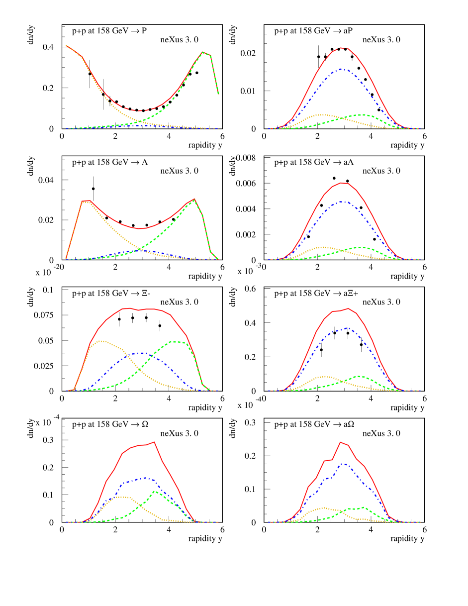
Figure 17: Rapidity spectra of baryons and antibaryons calculated from NEXUS 3.0 (projectile remnant contribution: dashed lines; target remnant contribution: dotted lines;Pomeron contribution: dashed dotted lines; sum: solid lines) and NA49 experiment [1] (points).

References

- [1] T. Susa et al, NA49, Nucl. Phys. A698 (2002) 491c; K. Kadija, talk given at Strange Quark Matter 2001, Frankfurt, Germany.
- [2] K. Werner, Phys. Rept. 232 (1993) 87.
- [3] M. Bleicher et al., J. Phys. G 25 (1999) 1859. [arXiv:hep-ph/9909407].
- [4] X. N. Wang, Phys. Rept. 280 (1997) 287. [arXiv:hep-ph/9605214].
- [5] T. Sjostrand et al., Comput. Phys. Commun. 135 (2001) 238. [arXiv:hep-ph/0010017].
- [6] H. Pi, Comput. Phys. Commun. 71 (1992) 173.
- [7] J. Ranft, Z. Phys. C 43 (1989) 439; A. Capella et al., Phys. Rept. 236 (1994) 225.
- [8] A. B. Kaidalov et al., Phys. Lett. B 117 (1982) 247.
- [9] M. Bleicher et al., Phys. Rev. Lett. 88, 202501 (2002) [arXiv:hep-ph/0111187].
- [10] H. J. Drescher et al., Phys. Rept. 350 (2001) 93. [arXiv:hep-ph/0007198].
- [11] K. Werner and J. Aichelin, Phys. Rev. C52 (1995) 9503021.
.