OSU-HEP-02-01

Collider Implications of Universal Extra Dimensions
C. Macesanu, C.D. McMullen and S. Nandi

Department of Physics, Oklahoma State University
Stillwater, OK  74078, USA

We consider the universal extra dimensions scenario of Appelquist, Cheng, and Dobrescu, in which all of the SM fields propagate into one extra compact dimension, estimated therein to be as large as $\sim(350$ GeV$)^{-1}$. Tree-level KK number conservation dictates that the associated KK excitations can not be singly produced. We calculate the cross sections for the direct production of KK excitations of the gluon, $g_{n}^{\star}$, and two distinct towers of quarks, $q_{n}^{\bullet}$ and $q_{n}^{\circ}$, in proton-antiproton collisions at the Tevatron Run I and II energies in addition to proton-proton collisions at the Large Hadron Collider energy. The experimental signatures for these processes depend on the stability of the lowest-lying KK excitations of the gluons and light quarks. We find that the Tevatron Run I mass bound for KK quark and gluon final states is about $350$–$400$ GeV, while Run II can push this up to $450$–$500$ GeV at its initial luminosity and $500$–$550$ GeV if the projected final luminosity is reached. The LHC can probe much further: The LHC will either discover UED KK excitations of quarks and gluons or extend the mass limit to about $3$ TeV.

1. Introduction

The low-energy phenomenology of superstring-inspired models with large extra compact dimensions depends on the mechanism of new physics by which the Standard Model (SM) fields are constrained, if at all, to motion in the usual $3$D wall (D₃ brane) of the usual three spatial dimensions. It might naively be speculated that as more SM fields are free to propagate into the extra compact dimensions (the bulk), then the collider bounds on the compactification scale would significantly strengthen. A non-universal model where the gauge bosons propagate into the bulk, but the fermions are confined to the usual SM D₃ brane, for example, does produce more stringent collider bounds than a model where all of the SM fields are confined to the D₃ brane. However, scenarios with universal extra dimensions (UED), in which all of the SM fields propagate into the bulk, have much weaker collider bounds. This is due to tree-level Kaluza-Klein (KK) number conservation, which dictates that colliding SM initial states can not produce single KK excitations and also forbids tree-level indirect collider effects. In the non-universal scenarios, the SM fields that are confined to the D₃ brane appear in the Lagrangian with delta functions, thereby permitting couplings that violate KK number conservation.

Only the gravitons propagate into the extra compact dimensions in the class of models based on the approach of Arkani-Hamed, Dimopoulos, and Dvali (ADD) [1], where the compactification is symmetric – i.e., all of the $N$ extra dimensions have the same compactification radius $R$. The string scale $M_{D}$ is much smaller than the four-dimensional Planck scale $M_{P}$ [2], which are related by $M_{P}^{2}=M_{D}^{N+2}R^{N}$. Any SM fields that propagate into the bulk would have (KK) excitations with masses at the $10$ MeV scale or less. The non-observation of such states up to about a TeV implies, in this class of models, that all of the SM fields are confined to the usual SM D₃ brane. Hence, the only source of new contributions to collider processes arises from the KK excitations of the graviton. Although the contributions of individual KK modes, with $4$D gravitational strength, to collider processes is extremely small, a very large number of such modes contribute in a TeV-scale collider process because the compactification scale $\mu$ is so small ($\mu\sim$ mm${}^{-1}\sim 10^{-3}$ eV). The net KK effect can cause a significant deviation from the SM production rates. Bounds on the string scale from analyses of various collider processes are typically on the order of a TeV [3, 4] for these symmetric compactification models.

One way to permit some or all of the SM fields to propagate into the bulk is to relax the constraint that the extra compact dimensions be symmetric. Let us first consider the case where only the SM gauge bosons propagate into the bulk. As an example, it is possible to devise a model with asymmetrical compactification with five TeV^-1-size extra compact dimensions and one mm-size extra dimension, where the SM gauge bosons (and perhaps the Higgs boson) propagate into one of the TeV^-1-size dimensions. It was shown in Ref. [5] that this model satisfies all of the current astrophysical and cosmological constraints [6]. These asymmetric scenarios have a more direct effect in high-energy collider processes. Originating with the suggestion by Antoniadis [7], some of the studies that have been done for the collider phenomenology of the scenario in which the SM gauge bosons can propagate into the bulk, but where the SM fermions can not [8], include: the effects on electroweak (EW) precision measurements [9], Drell-Yan processes in hadronic colliders [10], $\mu^{+}\mu^{-}$ pair production in electron-positron colliders [10], EW processes in very high-energy electron-positron colliders [11], and multijet production in very high-energy hadronic colliders [12]. The typical bound on the compactification scale is $1$–$2$ TeV.

The UED model, where all of the SM fields propagate into one or more extra compact dimensions, may intuitively seem more natural than selectively confining SM fields to the usual SM D₃ brane. This scenario may be thought of as a generalization of the usual SM wall to a D_3+N brane, where $N$ represents the number of extra compact dimensions into which the SM fields propagate. In this universal model of Appelquist, Cheng, and Dobrescu [13], KK number conservation governs all of the couplings involving KK excitations. In particular, each such vertex involves at least two KK excitations. At the tree-level, then, KK effects can not manifest themselves indirectly at colliders, and direct production is only possible in pairs of KK states. Although KK number conservation is broken at the one-loop level, the lowest-lying KK excitations of the light fermions and the massless gauge bosons do not decay to the SM zero-modes at any order without a special mechanism to support this decay. Thus, the lowest-lying KK excitations of the light fermions and the massless gauge bosons may be completely stable. Possible decay mechanisms have been proposed in the literature [13, 14, 15]. Collider bounds for this universal scenario are comparatively light: The current mass bound [13, 15, 16] for the first KK excited modes is relatively low ($\sim 350$-$400$ GeV).

In this work, we make a detailed study of the collider implications of the universal scenario, in which all of the SM fields propagate into one TeV^-1-size extra compact dimension. More specifically, we calculate the cross sections for the pair-production of KK excitations of the gluons, $g_{n}^{\star}$, and two distinct KK quark towers, $q_{n}^{\bullet}$ and $q_{n}^{\circ}$, in proton-antiproton collisions at the Tevatron Run I and II energy in addition to proton-proton collisions at the Large Hadron Collider (LHC) energy. The signatures of these KK excitations depend on the stability of the lowest-lying KK excitations of the light quarks and gluons. We find that the Tevatron Run I mass bound for KK quark and gluon final states is about $350$–$400$ GeV, while Run II can push this limit up to $450$–$550$ GeV, depending on the luminosity. The LHC can probe much further: The LHC will either discover UED KK excitations of the quarks and gluons or extend the mass limit to about $3$ TeV. The organization of our paper is as follows. We develop the key ingredients of our formalism in Section $2$, which is supplemented by additional details in the Appendix. We also present the Feynman rules involving the KK excitations of the gluons and quarks. Section $3$ contains our analytical expressions for the pair-production of KK excitations of the gluons and quarks. We treat the case of stable KK final states in Section $4$. Here we present our results for the production cross sections of pairs of stable KK excitations, and discuss how to search for their collider signatures. We discuss possible decay mechanisms in Section $5$. Our results for the case where the pair-produced KK final states decay may be found here, along with methods of searching for this associated collider phenomenology. We present our conclusions in Section $6$.

2. Formalism

We are interested in the collider implications of the universal scenario, in which all of the SM fields propagate into a single TeV^-1-size extra compact dimension. Our focus is on the tree-level parton subprocesses that involve the direct pair-production of KK excitations of gluons, $g_{n}^{\star}$, and two distinct KK quark towers, $q_{n}^{\bullet}$ and $q_{n}^{\circ}$. We begin by generalizing the usual $4$D Lagrangian density to its $5$D analog. We perform orbifold compactification and integrate over the fifth dimension $y$ to obtain the effective $4$D theory, which is the usual $4$D Lagrangian density plus new physics terms involving the KK excitations of the quark and gluon fields. These new terms provide the masses of the KK modes as well as the Feynman rules for the vertices and propagators involving KK excitations. We develop the key elements of our formalism here, while supplementary details are included in the Appendix.

We denote the $4$D SM quark multiplets for one generation by $Q_{L}^{\textnormal{SM}}(x)$, $U_{R}^{\textnormal{SM}}(x)$, and $D_{R}^{\textnormal{SM}}(x)$. For example, the first generation is:

$$Q_{L}^{\textnormal{SM}}(x)=q_{L}(x)=\left(\!\begin{array}[]{c}u(x)\\ d(x)\end{array}\!\right)_{\!L}\,,\;\;U_{R}^{\textnormal{SM}}(x)=u_{R}(x)\,,\;\;D_{R}^{\textnormal{SM}}(x)=d_{R}(x)\,.$$ (1)

Each $4$D state is a two-component Weyl spinor. The analogous $5$D quark multiplets consist of massless four-component vector-like quarks, which we denote by $Q(x,y)$, $U(x,y)$, and $D(x,y)$. When these $5$D fields are decomposed into $4$D fields, corresponding to each $4$D field are a left-handed and right-handed zero mode. Each mode is a two-component Weyl spinor in $4$ dimensions. Half of the zero modes, which are not present in the $4$D SM, may be projected out via the simple orbifold compactification choice, $S_{1}/Z_{2}$ $(Z_{2}$:$y\rightarrow-y)$. The gauge fields polarized along the usual SM directions must be even under $y\rightarrow-y$ such that the zero modes will correspond to the usual $4$D gauge fields, which implies that the gauge fields polarized along the $y$ direction must be odd. For the quark fields, each of the KK $(n>0)$ modes for each multiplet will have a left-chiral and right-chiral part. The $Q_{L}^{n}(x)$, $U_{R}^{n}(x)$, and $D_{R}^{n}(x)$ components must be associated with the part of $Q(x,y)$, $U(x,y)$, and $D(x,y)$ that is even under $y\rightarrow-y$ in order to recover the appropriate SM chiral zero mode states. The remaining components, $Q_{R}^{n}(x)$, $U_{L}^{n}(x)$, and $D_{L}^{n}(x)$, must be associated with the part of $Q(x,y)$, $U(x,y)$, and $D(x,y)$ that is odd under $y\rightarrow-y$ such that the zero modes not observed in the SM will be projected out. Each of the $5$D multiplets $Q(x,y)$, $U(x,y)$, and $D(x,y)$ can therefore be Fourier expanded in terms of the compactified dimension $y$ as

$$Q(x,y) \!\!\!= \!\!\!\frac{1}{\sqrt{\pi R}}\left\{\left(\!\begin{array}[]{c}u(x)\\ d(x)\end{array}\!\right)_{\!L}+\sqrt{2}\sum_{n=1}^{\infty}\left[Q_{L}^{n}(x)\cos\left(\frac{ny}{R}\right)+Q_{R}^{n}(x)\sin\left(\frac{ny}{R}\right)\right]\right\}$$ (4)

$$U(x,y) \!\!\!= \!\!\!\frac{1}{\sqrt{\pi R}}\left\{u_{R}(x)+\sqrt{2}\sum_{n=1}^{\infty}\left[U_{R}^{n}(x)\cos\left(\frac{ny}{R}\right)+U_{L}^{n}(x)\sin\left(\frac{ny}{R}\right)\right]\right\}$$ (5)

$$D(x,y) \!\!\!= \!\!\!\frac{1}{\sqrt{\pi R}}\left\{d_{R}(x)+\sqrt{2}\sum_{n=1}^{\infty}\left[D_{R}^{n}(x)\cos\left(\frac{ny}{R}\right)+D_{L}^{n}(x)\sin\left(\frac{ny}{R}\right)\right]\right\}\,.$$ (6)

The SM fermion masses arise from the Yukawa couplings through the Higgs vacuum expectation value (VEV), while the KK modes receive mass from the kinetic term in the $5$D Lagrangian density as well as from the Yukawa couplings via the Higgs VEV’s. We first calculate the mass arising from the kinetic term. The $5$D Lagrangian density for the kinetic terms and interactions of the $5$D gluon field $A_{M}^{a}(x,y)$ with the $5$D $Q(x,y)$ fields are:

$$\mathcal{L}_{5}=i\bar{Q}(x,y)\left\{\Gamma^{M}\left[\partial_{M}+ig_{{}_{5}}T^{a}A_{M}^{a}(x,y)\right]\right\}Q(x,y)\,.$$ (7)

Here, $g_{{}_{5}}$ is the $5$D strong coupling, $M$ is the $5$D analog of the Lorentz index $\mu$, i.e., $M\in\{\mu,4\}$, and the $5$D gluon fields $A_{M}^{a}(x,y)$ can be Fourier expanded in terms of the compactified extra dimension $y$ as:

$$A_{\mu}^{a}(x,y)=\frac{1}{\sqrt{\pi R}}\left[A_{\mu 0}^{a}(x)+\sqrt{2}\sum_{n=1}^{\infty}A_{\mu,n}^{a}(x)\cos(\frac{ny}{R})\right]$$ (8)

$$A_{4}^{a}(x,y)=\frac{\sqrt{2}}{\sqrt{\pi R}}\sum_{n=1}^{\infty}A_{4,n}^{a}(x)\sin(\frac{ny}{R})\,.$$ (9)

The normalization of $A_{0}^{a}(x)$ is one-half that of the $n>0$ modes, necessary to obtain canonically normalized kinetic energy terms for the gluon fields in the effective $4$D Lagrangian density [17]. As previously stated, under the transformation $y\rightarrow-y$, the decomposed gluon fields transform as $A_{\mu}^{a}(x,-y)=A_{\mu}^{a}(x,y)$ and $A_{4}^{a}(x,-y)=-A_{4}^{a}(x,y)$. We choose to work in the unitary gauge, where we can apply the gauge choice $A_{4,n}^{a}(x)=0$ [18].

Integrating the kinetic part of Eq. (7) over the compactified dimension $y$ yields the $4$D Lagrangian density, and similarly for $U(x,y)$ and $D(x,y)$. This effective $4$D Lagrangian density consists of the usual kinetic terms for the SM fields, kinetic terms for the massive Dirac spinors $Q^{n}(x)$, $U^{n}(x)$, and $D^{n}(x)$, and mass terms for the KK excitations with mass $M_{n}^{\mathit{KK}}=n/R=n\mu$, where $\mu$ is the compactification scale, $1/R$.

Thus, in the absence of the Higgs mechanism, the KK excitations have masses given by $M_{n}=M_{n}^{\mathit{KK}}=n/R=n\mu$. Additional mass contributions from the Yukawa couplings of the $5$D quark multiplets via the Higgs VEV’s are obtained by writing the $5$D Lagrangian density for the couplings of the $5$D quark multiplets to the $5$D Higgs field, Fourier expanding these $5$D fields in terms of the compactified dimension $y$, and integrating over the extra dimension. The eigenvalues of the resulting mass matrix give the net mass $M_{n}$ of the KK modes in terms of the mass of the corresponding quark field $M_{q}$ and the mass from the compactification $M_{n}^{\mathit{KK}}$:

$$M_{n}=\sqrt{(M_{n}^{\mathit{KK}})^{2}+M_{q}^{2}}\,.$$ (10)

Relative to the compactification scale, the SM quark masses are negligible except for the top mass $M_{t}$.

The QCD interactions involving KK excitations include purely gluonic couplings as well as couplings with quark fields. The purely gluonic case was discussed in detail in Ref. [12], and the resulting couplings are identical to those of this universal scenario. We therefore refer the reader to this prior work for these details, and concentrate on the couplings of quark fields to gluon fields. The Feynman rules for the QCD interactions involving the KK excitations of the gluons and the two towers of KK excitations corresponding to each of the quark fields can be obtained by integrating the second part of Eq. (7) over the compactified dimension $y$ via Fourier expansion of the $5$D fields in terms of $y$, and similarly for $U(x,y)$ and $D(x,y)$.

Each KK $q_{n}^{\bullet}$ and $q_{n}^{\circ}$ state is identified as a combination of $Q$, $U$, and $D$. In the limit of massless SM quarks, this combination can be expressed as:

$$Q_{L,R}^{n}(x)\equiv P_{L,R}\left(\!\begin{array}[]{c}u_{n}^{\bullet}(x)\\ d_{n}^{\bullet}(x)\end{array}\!\right)\,,\;\;U_{R,L}^{n}(x)\equiv P_{R,L}u_{n}^{\circ}\,,\;\;D_{R,L}^{n}(x)\equiv P_{R,L}d_{n}^{\circ}\,,$$ (11)

where the projection operators are defined as $P_{L,R}\equiv\frac{1}{2}(1\mp\gamma_{5})$. In general, there is an additional Yukawa contribution to the masses, in which the $U_{R}$ and $U_{L}$ fields contribute to the mass of the $q_{n}^{\bullet}$ via the Higgs VEV, and similarly for contributions to $q_{n}^{\circ}$ from $Q_{L}$ and $Q_{R}$. For example, taking the SM $c$ quark to be massless, the combination of the second-generation up-type quark component of the KK multiplet $Q_{2L}^{n}(x)$ with the second-generation up-type quark component of $Q_{2R}^{n}(x)$ is identified as the single KK charm quark $c^{\bullet}$, which receives KK mass $M_{n}=n\mu=1/R$ from the kinetic term. There is a second KK tower corresponding to the SM charm quark, which comes from $U_{2R}^{n}(x)$ and $U_{2L}^{n}(x)$, that we denote by $c^{\circ}$. By $g_{n}^{\star}$ we denote KK mode $n$ of the gluon, and by $q_{n}^{\bullet}$ and $q_{n}^{\circ}$ we denote KK mode $n$ of two distinct towers of KK excitations of a given SM quark field $q$. Each KK quark tower contains terms that are even and odd under $Z_{2}$ parity. However, in KK quark pair production, the KK final states will be polarized with helicity corresponding to their even states ($Q_{L}(x)$, $U_{R}(x)$, and $D_{R}(x)$)in the cross channels, and the components associated with the odd part of the $5$D fields ($Q_{R}(x)$, $U_{L}(x)$, and $D_{L}(x)$) will only show up in direct channel production. For KK quark-gluon production, the final KK states will again be polarized with helicity corresponding to the even states. This is because the projection operators ensure the conservation of $Z_{2}$ parity. Regarding our notation, $n$ will be strictly nonzero unless we explicitly state otherwise.

The detailed procedure for integrating over the fifth dimension $y$ to obtain, in the effective $4$D theory, the factors for the allowed vertices involving the $q_{n}^{\bullet}$ and $q_{n}^{\circ}$ fields may be found in the Appendix, and lead to the coupling strengths displayed in Fig. 1. The states with helicity corresponding to the odd states under $Z_{2}$ parity ($Q_{R}(x)$, $U_{L}(x)$, and $D_{L}(x)$) only appear in couplings involving $q_{n}^{\bullet}$ $q_{n}^{\bullet}$ or $q_{n}^{\circ}$$q_{n}^{\circ}$, and do not show up when a SM quark is present. A SM quark can only couple to KK states with helicity corresponding to the even states (($Q_{L}(x)$, $U_{R}(x)$, and $D_{R}(x)$). The triple KK vertices with $q_{n}^{\bullet}$ and $q_{n}^{\circ}$ fields involve the integration of three cosines for the even parts and one cosine and two sines for the odd parts. This latter integration results in a minus sign relative to the first one whenever the KK gluon is more massive than either KK quark, which results in the presence of a $\gamma_{5}$ in these vertices. Note also that the two towers $q_{n}^{\bullet}$ and $q_{n}^{\circ}$ do not couple to one another. The Feynman rules for the purely gluonic vertices are summarized in Ref. [12]. Notice that a single KK mode can not couple to SM fields. This is a consequence of the more general tree-level conservation of KK number, which dictates that $N$ KK modes, $n_{{}_{1}}$,$n_{{}_{2}}$,$\ldots$,$n_{{}_{N}}$, can only couple to one another if they satisfy the relation:

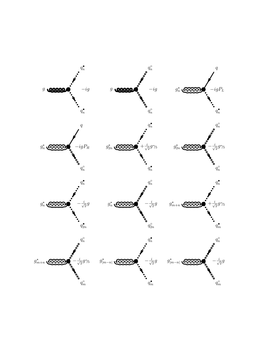
Figure 1: Relative coupling strengths of vertices involving $q_{n}^{\bullet}$’s and $q_{n}^{\circ}$’s. Only the overall factors are shown: These vertices also involve the usual SU($3$) matrix element and the Dirac $\gamma_{\mu}$ matrix. Here, $n$ and $m$ are distinct positive integers ($n\neq m$) and the projection operators are defined as $P_{L,R}\equiv(1\mp\gamma_{5})/2$.

$$\mid\!n_{{}_{1}}\,\pm\,n_{{}_{2}}\,\pm\,\cdots\,\pm\,n_{{}_{N-1}}\!\mid\,=n_{{}_{N}}\,.$$ (12)

KK number conservation strictly applies at every vertex, as well as for tree-level $N\rightarrow M$ processes, but is broken at the loop-level. The higher modes can therefore decay to the lower modes at the loop-level, but the lowest-lying KK modes of the light quarks and massless gluons will be completely stable unless there exists another form of new physics to serve as a decay mechanism. We will return to this point in Section $5$.

The $g_{n}^{\star}$ propagator is that of a usual massive gauge boson, shown here in the unitary gauge:

$$-i\Delta_{\mu\nu n}^{ab}(p^{2})=-i\delta^{ab}\frac{g_{\mu\nu}-\frac{p_{\mu}p_{\nu}}{M_{n}^{2}}}{p^{2}-M_{n}^{2}+iM_{n}\Gamma_{g}^{n}}\,.$$ (13)

Similarly, the $q_{n}^{\bullet}$ and $q_{n}^{\circ}$ propagators have the form of a usual massive quark:

$$-i\Delta_{n}^{a^{\prime}b^{\prime}}(p^{2})=i\delta^{a^{\prime}b^{\prime}}\frac{\not\!p+M_{n}}{p^{2}-M_{n}^{2}+iM_{n}\Gamma_{q}^{n}}\,.$$ (14)

The decay widths of the $g_{n}^{\star}$’s, $q_{n}^{\bullet}$’s, and $q_{n}^{\circ}$’s depend on stability of the lowest-lying KK excitations of the up quark, down quark, and gluon. However, these decay widths are immaterial for production processes, since KK number conservation forbids any $s$-channel KK propagators from arising in tree-level subprocesses with initial SM fields.

The mass of the $g_{n}^{\star}$ also enters into the expression for the cross section via summations over polarization states when external $g_{n}^{\star}$’s are involved. For the direct production of a $g_{n}^{\star}$, the summation of polarization states is given by

$$\sum_{\sigma}\epsilon_{\mu n}^{a\ast}(k,\sigma)\epsilon_{\nu n}^{b}(k,\sigma)=\mbox{\raisebox{-2.58334pt}{\huge$($}}\!\!-g_{\mu\nu}+\frac{k_{\mu}k_{\nu}}{M_{n}^{2}}\mbox{\raisebox{-2.58334pt}{\huge$)$}}\delta^{ab}\,.$$ (15)

For the case of external $g$’s, a projection such as

$$\sum_{\sigma}\epsilon_{\mu}^{a\ast}(k,\sigma)\epsilon_{\nu}^{b}(k,\sigma)=\mbox{\raisebox{-2.58334pt}{\huge$[$}}\!-g_{\mu\nu}+\frac{(\eta_{\mu}k_{\nu}+\eta_{\nu}k_{\mu})}{(\eta\cdot k)}-\frac{\eta^{2}k_{\mu}k_{\nu}}{(\eta\cdot k)^{2}}\mbox{\raisebox{-2.58334pt}{\huge$]$}}\delta^{ab}$$ (16)

can be made to eliminate unphysical longitudinal polarization states (and thereby satisfy gauge invariance), where $\eta_{\mu}$ is an arbitrary four-vector.

3. Pair Production of KK Excitations

We have in mind the production of pairs of KK excitations of the gluons, $g_{n}^{\star}$, and quarks, $q_{n}^{\bullet}$ and $q_{n}^{\circ}$, in proton-antiproton collisions at the Tevatron Run I or II energy or proton-proton collisions at the LHC energy. We focus on the parton subprocesses in this section and postpone numerical results to the following sections where the stability of the lowest-lying KK excitations is addressed. The various subprocesses are enumerated in Table 1. We perform our calculations at the tree-level, and restrict ourselves to two final states. Due to KK number conservation, not only must the KK excitations be produced in pairs, but they necessarily have the same mode $n$, which is the same mode that any KK propagators will have. We neglect the quark masses except for the top mass $M_{t}$, but neglect the content of top flavor in the colliding protons and antiprotons. Thus, the top quark only enters into the calculation of the cross sections for $gg\rightarrow q_{n}^{\bullet}\bar{q}_{n}^{\bullet}$ and $q\bar{q}\rightarrow q^{\prime}{}_{n}^{\bullet}\bar{q}^{\prime}{}_{n}^{\bullet}$, and the analogous subprocesses for the $q_{n}^{\circ}$’s. We also neglect the decay widths of all SM and KK particles in this section since massive propagators will not appear in the $s$-channel due to tree-level KK number conservation and our neglect of initial top quarks. We will incorporate the decay widths in the subsequent decay of the final states in Section $5$, where we discuss possible mechanisms for the decay of the lowest-lying KK states.

Table 1: Subprocesses leading to double KK production at hadronic colliders. Not shown are subprocesses that are simply related by the exchange of a particle and antiparticle, as in $\bar{q}g\rightarrow\bar{q}_{n}^{\bullet}g_{n}^{\star}$.

Double KK gluon production subprocesses consist of $gg\rightarrow g_{n}^{\star}g_{n}^{\star}$ and $q\bar{q}\rightarrow g_{n}^{\star}g_{n}^{\star}$. The former subprocess involves direct-channel SM gluon exchange, cross-channel KK gluon exchanges, and the four-point interaction. The latter subprocess is unique in that there are five tree-level Feynman diagrams, which include direct-channel SM gluon exchange and cross-channel $q_{n}^{\bullet}$ and $q_{n}^{\circ}$ exchanges. For the purely gluonic subprocess, the amplitude-squared, summed over final states and averaged over initial states, is:

$$\mbox{\raisebox{-2.15277pt}{\Large$\bar{\Sigma}$}}\left|{\cal M}(gg\rightarrow g_{n}^{\star}g_{n}^{\star})\right| = {9\over 4}\ g_{s}^{4}(Q)\left(1-{\hat{t}{{}^{\prime}}\hat{u}{{}^{\prime}}\over\hat{s}^{2}}\right)$$ (17)

$$\!\!\!\cdot \!\!\!\!\!\!\left[3\ +\ 2\frac{\hat{s}^{2}}{\hat{t}{{}^{\prime}}^{2}\hat{u}{{}^{\prime}}^{2}}\left(3M_{n}^{4}+\hat{s}^{2}\right)\ -\ 2\frac{\hat{s}}{\hat{t}{{}^{\prime}}\hat{u}{{}^{\prime}}}\left(3M_{n}^{2}+2\hat{s}\right)\right]\,,$$

where the strong coupling constant $g_{s}$ is evaluated at the scale $Q$ equal to the mass of the final state KK excitations $M_{n}$, and $\hat{v}^{\prime}$ represents subtraction of $M_{n}^{2}$ from the Mandelstam variable $\hat{v}\in\{\hat{s},\hat{t},\hat{u}\}$ (i.e., $\hat{v}^{\prime}=\hat{v}-M_{n}^{2}$). We note that $gg\rightarrow g_{n}^{\star}g_{n}^{\star}$ is the same in the UED scenario considered here as well as in a model where only gluons propagate into the bulk. However, each of the remaining subprocesses is different. The amplitude-squared for $q\bar{q}\rightarrow g_{n}^{\star}g_{n}^{\star}$ is:

$$\mbox{\raisebox{-2.15277pt}{\Large$\bar{\Sigma}$}}\!\mid\!\mathcal{M}(q\bar{q}\rightarrow g_{n}^{\star}g_{n}^{\star})\!\mid^{2}\,= \!\!\!\!\!\!\!\!\!\frac{2}{27}\ g_{s}^{4}(Q)\left[\frac{M_{n}^{2}}{\hat{s}}\left(-4\frac{\hat{s}^{4}}{\hat{t}{{}^{\prime}}^{2}\hat{u}{{}^{\prime}}^{2}}+57\frac{\hat{s}^{2}}{\hat{t}{{}^{\prime}}\hat{u}{{}^{\prime}}}-108\right)\right.$$ (18)

$$\!\!\!+ \!\!\!\!\left.20\frac{\hat{s}^{2}}{\hat{t}{{}^{\prime}}\hat{u}{{}^{\prime}}}-93+108\frac{\hat{t}{{}^{\prime}}\hat{u}{{}^{\prime}}}{\hat{s}^{2}}\right]\,.$$

KK quark-gluon production results from $qg\rightarrow q_{n}^{\bullet}g_{n}^{\star}$ and $qg\rightarrow q_{n}^{\circ}g_{n}^{\star}$. (We will not enumerate subprocesses that are simply related by particle-antiparticle replacement, such as $\bar{q}g\rightarrow\bar{q}_{n}^{\bullet}g_{n}^{\star}$.) These subprocesses involve $s$-channel SM quark exchange, $t$-channel $g_{n}^{\star}$ exchange, and $u$-channel KK quark exchange. The square of the matrix element for $qg\rightarrow q_{n}^{\bullet}g_{n}^{\star}$ is:

$$\mbox{\raisebox{-2.15277pt}{\Large$\bar{\Sigma}$}}\!\mid\!\mathcal{M}(qg\rightarrow q_{n}^{\bullet}g_{n}^{\star})\!\mid^{2}\,= \!\!\!\!\!\!\!\!\!\frac{-1}{3}\ g_{s}^{4}(Q)\left(\frac{5\hat{s}^{2}}{12\hat{t}{{}^{\prime}}^{2}}+\frac{\hat{s}^{3}}{\hat{t}{{}^{\prime}}^{2}\hat{u}{{}^{\prime}}}+\frac{11\hat{s}\hat{u}{{}^{\prime}}}{6\hat{t}{{}^{\prime}}^{2}}+\frac{5\hat{u}{{}^{\prime}}^{2}}{12\hat{t}{{}^{\prime}}^{2}}+\frac{\hat{u}{{}^{\prime}}^{3}}{\hat{s}\hat{t}{{}^{\prime}}^{2}}\right)\,.$$ (19)

The subprocess $qg\rightarrow q_{n}^{\circ}g_{n}^{\star}$ is identical to $qg\rightarrow q_{n}^{\bullet}g_{n}^{\star}$. That is, the sign of the $\gamma_{5}$ matrix is not important in KK quark production unless both $q_{n}^{\bullet}$ and $q_{n}^{\circ}$ are involved in the same subprocess, e.g., in $q\bar{q}\rightarrow g_{n}^{\star}g_{n}^{\star}$ or $qq\rightarrow q_{n}^{\bullet}q_{n}^{\circ}$.

Subprocesses with identical final $q_{n}^{\bullet}$ or $q_{n}^{\circ}$ states feature $t$- and $u$-channel $g_{n}^{\star}$ exchanges. A relative minus sign represents the antisymmetrization of fermionic wave functions that originates from the interchange of identical fermionic states between the two diagrams. Notice that although a given SM quark $q$ and its KK counterparts have different mass, they have the same fermionic properties that produces the minus sign for the antisymmetrization of wave functions. The amplitude-squared for $q_{n}^{\bullet}q_{n}^{\bullet}$ production is:

$$\mbox{\raisebox{-2.15277pt}{\Large$\bar{\Sigma}$}}\!\mid\!\mathcal{M}(qq\rightarrow q_{n}^{\bullet}q_{n}^{\bullet})\!\mid^{2}\,= \!\!\!\!\!\!\!\!\!\frac{1}{27}\ g_{s}^{4}(Q)\left[\frac{M_{n}^{2}}{\hat{s}}\left(-6\frac{\hat{s}^{4}}{\hat{t}{{}^{\prime}}^{2}\hat{u}{{}^{\prime}}^{2}}+17\frac{\hat{s}^{2}}{\hat{t}{{}^{\prime}}\hat{u}{{}^{\prime}}}\right)\right.$$ (20)

$$\!\!\!+ \!\!\!\!\left.6\frac{\hat{s}^{4}}{\hat{t}{{}^{\prime}}^{2}\hat{u}{{}^{\prime}}^{2}}-16\frac{\hat{s}^{2}}{\hat{t}{{}^{\prime}}\hat{u}{{}^{\prime}}}+2\right]\,.$$

The identical result is obtained for $q_{n}^{\circ}q_{n}^{\circ}$ production.

Double KK quark-antiquark pairs with the same flavor can arise from initial gluons or quarks. The former case involves direct-channel SM gluon exchange and cross-channel KK quark exchanges. The latter case consists of $s$-channel SM gluon exchange, and, in the case of initial partons of the same flavor as the final states, $t$-channel $g_{n}^{\star}$ exchange. For initial gluons, squaring the amplitude leads to the following expression for KK quark pair production:

$$\mbox{\raisebox{-2.15277pt}{\Large$\bar{\Sigma}$}}\!\mid\!\mathcal{M}(gg\rightarrow q_{n}^{\bullet}\bar{q}_{n}^{\bullet})\!\mid^{2}\,= \!\!\!\!\!\!\!\!\!g_{s}^{4}(Q)\left[\left(\frac{M_{n}^{4}}{\hat{t}{{}^{\prime}}\hat{u}{{}^{\prime}}}-\frac{M_{n}^{2}}{\hat{s}}\right)\left(\frac{3}{2}-\frac{2\hat{s}^{2}}{3\hat{t}{{}^{\prime}}\hat{u}{{}^{\prime}}}\right)\right.$$ (21)

$$\!\!\!+ \!\!\!\!\left.\frac{\hat{s}^{2}}{6\hat{t}{{}^{\prime}}\hat{u}{{}^{\prime}}}-\frac{17}{24}+\frac{3\hat{t}{{}^{\prime}}\hat{u}{{}^{\prime}}}{4\hat{s}^{2}}\right]\,,$$

where the only difference for the case of KK top pair production is adjustment of the mass via Eq. 10. The amplitude-squared for KK quark-antiquark final states arising from SM quark-antiquark initial states, for which the flavor is the same in the initial and final states, is:

$$\mbox{\raisebox{-2.15277pt}{\Large$\bar{\Sigma}$}}\!\mid\!\mathcal{M}(q\bar{q}\rightarrow q_{n}^{\bullet}\bar{q}_{n}^{\bullet})\!\mid^{2}\,= \!\!\!\!\!\!\!\!\!\frac{1}{54}\ g_{S}^{4}(Q)\left[\frac{M_{n}^{2}}{\hat{s}}\left(48-12\frac{\hat{s}}{\hat{t}{{}^{\prime}}}+12\frac{\hat{s}^{2}}{\hat{t}{{}^{\prime}}^{2}}\right)\right.$$ (22)

$$\!\!\!+ \!\!\!\!\left.48\frac{\hat{t}{{}^{\prime}}^{2}}{\hat{s}^{2}}+36\frac{\hat{t}{{}^{\prime}}}{\hat{s}}+23+16\frac{\hat{s}}{\hat{t}{{}^{\prime}}}+12\frac{\hat{s}^{2}}{\hat{t}{{}^{\prime}}^{2}}\right]\,.$$

This does not lead to KK top quark production since the top quark content of the colliding protons is negligible. The relative sign between the two diagrams again incorporates the antisymmetrization of fermionic wave functions corresponding to the interchange of two fermionic states between the two diagrams. When the final states have different flavors than the initial state, only the $s$-channel contributes. For the lighter flavors, this is simply the $s$-channel part of Eq. 22:

$$\mbox{\raisebox{-2.15277pt}{\Large$\bar{\Sigma}$}}\!\mid\!\mathcal{M}(q\bar{q}\rightarrow q^{\prime}{}_{n}^{\bullet}\bar{q}^{\prime}{}_{n}^{\bullet})\!\mid^{2}\,= \!\!\!\!\!\!\!\!\!\frac{4}{9}\ g_{s}^{4}(Q)\left(2\frac{M_{n}^{2}}{\hat{s}}-2\frac{\hat{t}{{}^{\prime}}\hat{u}{{}^{\prime}}}{\hat{s}^{2}}+1\right)\,.$$ (23)

Again, for top production, the only change involves correcting for the final state KK mass. The same results apply for $q_{n}^{\circ}\bar{q}_{n}^{\circ}$ production.

For double KK quark production with different flavors in the final state, the result is the same as the corresponding case with identical flavors with the appropriate channel removed. That is, $qq^{\prime}\rightarrow q_{n}^{\bullet}q^{\prime}{}_{n}^{\bullet}$ is just the $t$-channel contribution to $qq\rightarrow q_{n}^{\bullet}q_{n}^{\bullet}$,

$$\mbox{\raisebox{-2.15277pt}{\Large$\bar{\Sigma}$}}\!\mid\!\mathcal{M}(qq^{\prime}\rightarrow q_{n}^{\bullet}q^{\prime}{}_{n}^{\bullet})\!\mid^{2}\,= \!\!\!\!\!\frac{2}{9}\ g_{s}^{4}(Q)\left(-M_{n}^{2}\frac{\hat{s}}{\hat{t}{{}^{\prime}}^{2}}+\frac{1}{4}+\frac{\hat{s}^{2}}{\hat{t}{{}^{\prime}}^{2}}\right)\,,$$ (24)

while $q\bar{q}^{\prime}\rightarrow q_{n}^{\bullet}\bar{q}^{\prime}{}_{n}^{\bullet}$ is also the $t$-channel contribution to $q\bar{q}\rightarrow q_{n}^{\bullet}\bar{q}_{n}^{\bullet}$,

$$\mbox{\raisebox{-2.15277pt}{\Large$\bar{\Sigma}$}}\!\mid\!\mathcal{M}(q\bar{q}^{\prime}\rightarrow q_{n}^{\bullet}\bar{q}^{\prime}{}_{n}^{\bullet})\!\mid^{2}\,= \!\!\!\!\frac{1}{18}\ g_{s}^{4}(Q)\left(4M_{n}^{2}\frac{\hat{s}}{\hat{t}{{}^{\prime}}^{2}}+4\frac{\hat{s}^{2}}{\hat{t}{{}^{\prime}}^{2}}+8\frac{\hat{s}}{\hat{t}{{}^{\prime}}}+5\right)\,,$$ (25)

and similarly for $q_{n}^{\circ}$ final states.

Finally, it is possible to produce the mixed KK final states involving one $q_{n}^{\bullet}$ and one $q_{n}^{\circ}$. The projection operators conspire to nullify the interference term in $qq\rightarrow q_{n}^{\bullet}q_{n}^{\circ}$. The differing signs of the $\gamma_{5}$’s also affect the $t$- and $u$-channel contributions. The amplitude-squared for this subprocess is:

$$\mbox{\raisebox{-2.15277pt}{\Large$\bar{\Sigma}$}}\!\mid\!\mathcal{M}(qq\rightarrow q_{n}^{\bullet}q_{n}^{\circ})\!\mid^{2}\,= \!\!\!\!\!\!\!\!\!\frac{1}{9}\ g_{s}^{4}(Q)\left[\frac{2M_{n}^{2}}{\hat{s}}\frac{\hat{s}^{2}}{\hat{t}{{}^{\prime}}\hat{u}{{}^{\prime}}}\left(\frac{\hat{s}^{2}}{\hat{t}{{}^{\prime}}\hat{u}{{}^{\prime}}}-2\right)\right.$$ (26)

$$\!\!\!+ \!\!\!\!\left.2\frac{\hat{s}^{4}}{\hat{t}{{}^{\prime}}^{2}\hat{u}{{}^{\prime}}^{2}}-8\frac{\hat{s}^{2}}{\hat{t}{{}^{\prime}}\hat{u}{{}^{\prime}}}+5\right]\,.$$

The six remaining mixed subprocesses, $q_{n}^{\bullet}\bar{q}_{n}^{\circ}$, $q_{n}^{\circ}\bar{q}_{n}^{\bullet}$, $q_{n}^{\bullet}q^{\prime}{}_{n}^{\circ}$, $q_{n}^{\circ}q^{\prime}{}_{n}^{\bullet}$, $q_{n}^{\bullet}\bar{q}^{\prime}{}_{n}^{\circ}$, and $q_{n}^{\circ}\bar{q}^{\prime}{}_{n}^{\bullet}$, all are represented by the same $t$-channel diagram and have the same form as the $t$-channel contribution to Eq. 26:

$$\mbox{\raisebox{-2.15277pt}{\Large$\bar{\Sigma}$}}\!\mid\!\mathcal{M}(q\bar{q}^{\prime}\rightarrow q_{n}^{\bullet}\bar{q}^{\prime}{}_{n}^{\bullet})\!\mid^{2}\,= \!\!\!\!\!\!\!\!\!\frac{1}{9}\ g_{s}^{4}(Q)\left[2\frac{M_{n}^{2}}{\hat{t}{{}^{\prime}}}\left(1+\frac{\hat{u}{{}^{\prime}}}{\hat{t}{{}^{\prime}}}\right)+\frac{5}{2}+4\frac{\hat{u}{{}^{\prime}}}{\hat{t}{{}^{\prime}}}+2\frac{\hat{u}{{}^{\prime}}^{2}}{\hat{t}{{}^{\prime}}^{2}}\right]\,.$$ (27)

It is not possible to produce mixed KK final states from initial gluons, nor is it possible to produce mixed KK final states of a different flavor from initial $q\bar{q}$ pairs.

These amplitude-squared formulae do not contain any terms that grow with energy, and the matrix elements for these subprocesses are tree-unitary. This has also been observed for the case in which only the gauge bosons propagate into the bulk [12, 20]. Note that the matrix elements of the individual diagrams with external gluons are not tree-unitary: There are delicate cancellations involved between individual diagrams, which ensures unitarity for the total amplitude. As an example, consider the subprocess, $q\bar{q}\rightarrow g_{n}^{\star}g_{n}^{\star}$, which has both $q_{n}^{\bullet}$ and $q_{n}^{\circ}$ propagators. The amplitude-squared for this reaction would not be tree-unitary if there were just a single tower of KK excitations of the quarks, or if the two towers $q_{n}^{\bullet}$ and $q_{n}^{\circ}$ did not couple left- and right-handedly to the SM quarks. This is another example of tree-unitarity for a class of massive vector boson theories other than the known spontaneously broken gauge theories [21].

4. Stable KK Excitations

As previously discussed, the lowest-lying KK excitations of the light fermions and massless gauge fields may very well be stable. This is a consequence of KK number conservation (Eq. 12), which is valid at all vertices and thus also at the tree-level. KK number is broken at the loop-level, but the lowest lying KK excitations of massless gauge bosons and the light fermions can not decay even at the loop level unless some new physics mechanism is introduced. The KK excitations of massive gauge bosons and heavier generation fermions can decay to lighter KK states and SM fields at tree-level. For any SM decay with a massless final state, such as $Z\rightarrow\nu\bar{\nu}$, there are corresponding decays involving their KK excitations, such as $Z_{1}^{\star}\rightarrow\nu_{1}^{\bullet}\bar{\nu}$. When the final states are massive the decay may be kinematically forbidden, depending on the compactification scale: For example, the $t_{1}^{\bullet}$ can not decay to $W^{+}b_{1}^{\bullet}$ for a $400$ GeV compactification scale, but it can decay to $W_{1}^{+\star}b$. At the tree-level, KK number conservation results in increasing kinematic suppression of all decays involving KK excitations of massive SM fields with increasing compactification scale. Note also that the lowest-lying KK excitations of the quarks and gluons can not decay to their SM counterparts via graviton emission unless KK number is violated in such interactions. We consider the hadronic collider phenomenology of stable or long-lived $n=1$ KK excitations in this section, then turn our attention to new physics mechanisms that may result in short-lived lowest-lying KK states and their associated phenomenology in the next section. By long-lived, we refer to lifetimes long enough such that the final state decay occurs beyond the detector.

For stable KK final states, the production cross sections for the set of subprocesses $\{j\}$ enumerated in the previous section are related to the squares of the amplitudes tabulated therein via:

$$\sigma_{{}_{\mathit{KK}}}^{\mathit{tot}}=\frac{1}{4\pi} \!\!\!\!\!\!\!\sum_{j}\sum_{n}\,\,\,\,\int_{\mbox{\raisebox{-4.52083pt}{\scriptsize{$\!\!\!\!\!\!\!\!\rho_{n}$}}}}^{\mbox{\raisebox{2.71246pt}{\scriptsize{$\!\!\!1$}}}}dx_{{}_{A}}\int_{\mbox{\raisebox{-4.52083pt}{\scriptsize{$\!\!\!\!\!\!\!\!\!\!\rho_{n}/x_{{}_{A}}$}}}}^{\mbox{\raisebox{2.71246pt}{\scriptsize{$\!\!\!1$}}}}\!\!\!\!dx_{{}_{B}}f_{a/{}_{A}}(x_{{}_{A}},Q)f_{b/{}_{B}}(x_{{}_{B}},Q)$$ (28)

$$\!\!\int_{\mbox{\raisebox{-3.91806pt}{\scriptsize{$\!\!\!\!\!\!-1$}}}}^{\mbox{\raisebox{2.71246pt}{\scriptsize{$\!\!\!1$}}}}dz\,\frac{\mbox{\raisebox{-2.15277pt}{\Large$\bar{\Sigma}$}}\!\mid\!M_{j}\!\mid^{2}}{S!}\,\frac{1}{\hat{s}}\sqrt{1-\frac{4M_{n}^{2}}{\hat{s}}}\,,$$

where $S$ is a statistical factor (the number of identical final states) and $\rho_{n}=4M_{n}^{2}/s$. The first summation is over the subprocesses $\{j\}$ tabulated in the previous section, while the second summation runs over all $n$ for which pairs of final states with mass $M_{n}$ can be produced for a given collider energy $\sqrt{s}$. The higher ($n>1$) states produce only a slight effect (at the $1\%$ level) due to their large mass. The cross sections for the higher modes are easily computed from the cross section expression for the first mode by simply replacing the mass of the first mode with that of the higher mode, which includes adjusting the scale $Q$ to correspond to the higher mass.

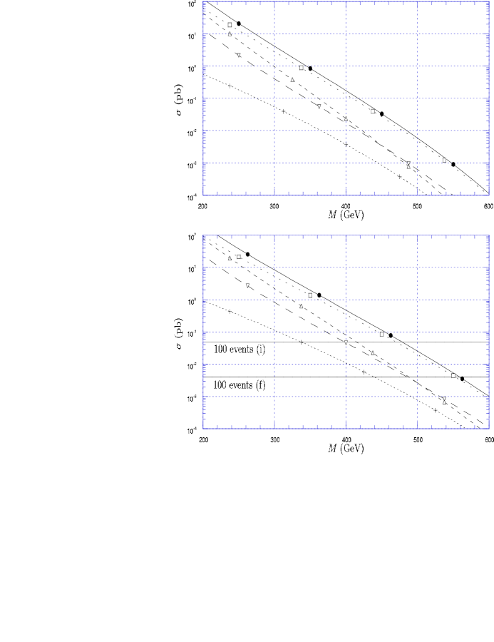
Figure 2: The cross section for the production of two stable KK final states is shown as a function of the KK mass for Tevatron Run I (top) and II (bottom). The solid curve corresponds to the total contribution, while the dashed lines represent the partial contributions of KK quark pair ($\square$), KK quark-gluon ($\vartriangle$), and KK gluon pair ($\triangledown$) production. Also shown is top production ($+$), which features a different collider signature (namely, the top will subsequently decay into additional states). Solid horizontal lines mark $100$ events at the initial and final projected luminosities for Run II.

We evaluate the cross sections in Eq. 28 with the CTEQ$5$ distribution functions [25] and $Q=M_{n}$ in the parton luminosity. In Fig. 2, we present the cross section for the production of two stable KK final states for a given first excited KK mass $M=\mu=1/R$ at the Tevatron proton-antiproton collider. In addition to the total cross section, the contributions of KK gluon pair, KK quark-gluon, and KK quark pair production are plotted. For the case of double KK quark production, the final state consists of light quark KK excitations, but not the top quark, which can decay (e.g., $t_{1}^{\circ}\rightarrow W_{1}^{+\star}b$). The production of KK quark pairs is dominant (not as much because the cross section for a specific process is much higher, but because there are many more processes involved), while the KK gluon pair and KK quark-gluon production rates are comparable.

Stable, slowly moving KK quarks produced at colliders will hadronize, producing high-ionization tracks. The production of numerous heavy, charged stable particles will produce a clear signal of new physics. They will appear as a heavy replica of the light SM quarks, with both up- and down-type quark charges, but with two KK quarks corresponding to each SM quark.

At the Tevatron Run I, searches for heavy stable quarks [26] have set an upper limit of about $1$ pb on the production cross section of such particles (for a mass range between $200$ and $250$ GeV). Using a naive extrapolation of the limits presented in Ref. [26] to higher mass values, we estimate a lower bound on the first excited KK mass of about $350$ GeV (in agreement with Ref. [13]). For the projected initial (final) Run II ($\sqrt{s}=2$ TeV) integrated luminosity, which will yield $2$ ($25$) events for each $10^{-3}$ pb of cross section, $100$ events would be produced for a compactification scale of $450$ GeV ($550$ GeV). In order to set definite limits on the mass of KK excitations at Run II, an analysis similar to the one performed for Run I is needed. An estimate of the Run II reach can be made by assuming that the limit on the heavy stable quarks production cross-section is driven by statistics. In this case, we can expect an improvement of around a factor of $10$ in this limit, to $0.1$ pb. Then, the nonobservation of heavy stable quarks will raise the lower bound for the mass of the first KK mode in the universal scenario to around $450$ GeV.

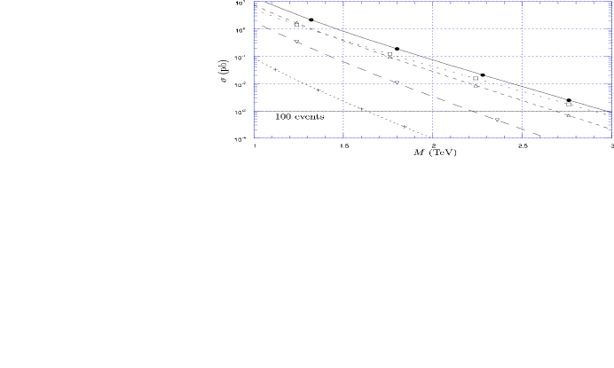
Figure 3: The same as Fig. 2, but for the LHC. The solid horizontal line represents $100$ annual events at the projected luminosity.

Much better prospects for the discovery of KK fields may be found at the LHC proton-proton collider, where the anticipated annual luminosity is $10^{5}$ pb^-1. The cross-sections for the production rate of two stable KK excitations at the LHC energy are illustrated in Fig. 3. A dedicated study is required to find the exact reach of the LHC in this case, but, by requiring at least $100$ events to be produced, we can estimate that the LHC will discover the first stable KK excitations if their mass is smaller than about $3$ TeV.

Thus, stable KK quarks and gluons of the UED scenario will either be discovered at the Tevatron Run II or the LHC, or the lower bound on their masses will be raised to around $450$ GeV or $3$ TeV, respectively. However, cosmological constraints require new physics to explain the existence of stable KK excitations in this mass range. This cosmological restriction can be lifted via a new physics mechanism that causes the lowest-lying KK excitations to have a lifetime that is short compared to the cosmological scale. We now focus on this possibility.

5. Decay Mechanisms

The lowest-lying KK excitations of the light fermions and the massless gauge bosons can decay into SM fields via new physics mechanisms that produce a violation in KK number conservation. Various decay schemes have been considered in the literature [14], [13], [15]. However, provided that the KK excitations decay within the detector, the effect of a specific decay mechanism on the final state distributions presented here can be expected to be small.

For purposes of illustration, we shall analyze in some detail the decay properties of KK excitations in the fat brane scenario proposed in Ref. [14]. In this scenario, the “small” universal extra dimension is assumed to be the thickness of the D₄ brane in which the SM particles propagate. In turn, this brane is embedded in a $4+N$ dimensional space, in which gravity propagates. (In order to avoid drastically modifying Newton’s law at the solar system scale, we require $N\geq 2$.) We take the gravity extra dimensions (call them $\{z_{i}\}$) to be symmetric, with a compactification radius $r$ much larger than the thickness of the fat brane $R$. The orbifold structure of the UED space in which the SM fields propagate can be imposed by using boundary conditions on the fat brane. The non-gravitational interactions are identical to those presented in the Appendix. The differences in this model lie in the interactions between gravity and the KK excitations of the SM fields, where KK number violation in such interactions will mediate the decays. The thick brane absorbs the unbalanced momentum that results from the KK number violation.

The effective $4$D interactions of the graviton fields with the SM fields and their KK excitations are obtained by the ‘naive’ (straightforward) generalization of the results in Ref. [4]. The Feynman rules for the couplings of the graviton fields to the UED fields are related to the corresponding couplings of the graviton fields to the SM fields by the form factor $\mathcal{F}_{n}(x_{y})$ as introduced in Ref. [14, 15]. For example, the $q_{n}^{\bullet}$-$q$-$G_{\vec{k}}$ coupling is:

$$\Lambda_{q_{n}^{\bullet}\mbox{-}q\mbox{-}G_{\vec{k}}}=\mathcal{F}_{n}(x_{y})\Lambda_{q\mbox{-}q\mbox{-}G_{\vec{k}}}\,,$$ (29)

where $G_{\vec{k}}$ is the KK excitation of the graviton corresponding to mode $\vec{k}$ and $x_{y}\equiv m_{y}R=2\pi k_{y}R/r$. Note that $n$ is the mode of the KK quark field, while $k_{y}$ is the mode of the KK graviton field along the $y$ direction. Thus, $m_{y}$ is the contribution of the $y$ dimension to the graviton mass. As with the non-gravitational interactions, the KK quark field components associated with odd $Z_{2}$ parity ($Q_{R}(x)$, $U_{L}(x)$, and $D_{L}(x)$) do not interact with the SM quark fields because of the presence of the projection operators. Thus, these KK fields associated with odd $Z_{2}$ parity can not decay to SM quarks and gravitons as indicated in Ref. [15]. The form factor, $\mathcal{F}_{n}(x)$, does not include the sine terms, and depends on the component of the graviton mass arising from the universal compact dimension only, $k_{y}$:

$$\mathcal{F}_{n}(x_{y})=\frac{\sqrt{2}}{\pi R}\int_{0}^{\pi R}dy\exp(\frac{i2\pi k_{y}y}{r})\cos(\frac{ny}{R})\,.$$ (30)

Our result for the modulus-square of form factor,

$$|\mathcal{F}_{1}(x_{y})|^{2}=\frac{4}{\pi^{2}}\frac{x_{y}^{2}}{(1-x_{y}^{2})^{2}}\left[1+\cos(\pi x_{y})\right]$$ (31)

differs by the sign of the cosine term from the one in Ref. [15], which is potentially significant, since it affects the leading behavior of the form factor in the critical regions: $x_{y}$ near zero (decay to light gravitons) and unity (decay to heavy gravitons).

The total decay width is obtained by summing over all possible graviton towers the partial decay width $\Gamma_{n}(x_{y},x_{z})$, where $x_{a}$ refers to all of the extra dimensions, $x_{y}$ denotes the universal direction, and $x_{z}$ is exclusive to gravity: $x_{a}^{2}=x_{z}^{2}+x_{y}^{2}$. The form-factor appears as a multiplicative constant in the partial width:

$$\Gamma_{n}(x_{y},x_{z})=|\mathcal{F}_{n}^{2}(x_{y})|\ \Gamma^{\prime}_{n}(x_{a})\,.$$ (32)

Replacing the KK sum with an integral over the density of graviton states [4], we obtain:

$$\Gamma_{\mathit{tot}}=\sum_{G,\Phi}\frac{2\pi^{\frac{N-1}{2}}\ M_{P}^{2}\ M^{N}}{\Gamma(\frac{N-1}{2})\ \ M_{D}^{N+2}}\int_{2\pi R/r}^{1}dx_{y}\ |\mathcal{F}_{n}^{2}(x_{y})|\ \int_{0}^{\sqrt{1-x_{y}^{2}}}x_{z}^{N-2}dx_{z}\ \Gamma^{\prime}_{n}(x_{a})\,.$$ (33)

Here, $M_{P}$ is the conventional $4$D Planck scale, while $M_{D}$ is the $(4+N)$-dimensional Planck scale and should not be more than one or two orders of magnitude above $1/R$ [23]. Note that $N$ is the number of extra compact dimensions seen by the graviton, as opposed to the number of universal dimensions, which we take to be one.

For completeness, we give here the partial decay widths appearing in Eq. 33. These results are based on the three-point vertex Feynman rules given in Ref. [4], with the masses of all particles (except gravitons) set to zero. The decay of the $q_{n}^{\bullet}$ (or $q_{n}^{\circ}$ ) into a SM quark and a massive spin 2 graviton $G^{a}$ has partial width, apart from the overall form factor, given by:

$$\Gamma^{\prime}{}_{n}(q_{n}^{\bullet}\rightarrow qG^{a})=\frac{\kappa^{2}}{768\pi}\frac{M_{n}^{3}}{x_{a}^{4}}\left[\left(1-x_{a}^{2}\right)^{4}\left(2+3x_{a}^{2}\right)\right]\,.$$ (34)

The $q_{n}^{\bullet}$ can also decay into one of $N(N-1)/2$ massive spin-$0$ particles, $\phi^{a}_{ij}$:

$$\Gamma^{\prime}_{n}(q_{n}^{\bullet}\rightarrow q\phi^{a}_{ij})=\delta_{ij}\frac{9\kappa^{2}\omega^{2}}{256\pi}M_{n}^{3}(1-x_{a}^{2})^{2}\,,$$ (35)

where $\omega=\sqrt{\frac{2}{3(N+2)}}$. Finally, the $g_{n}^{\star}$ can only decay into a SM gluon via massive spin 2 graviton emission:

$$\Gamma^{\prime}_{n}(g_{n}^{\star}\rightarrow gG^{a})=\frac{\kappa^{2}}{96\pi}\frac{M_{n}^{3}}{x_{a}^{4}}\left[\left(1-x_{a}^{2}\right)^{2}\left(1+3x_{a}^{2}+6x_{a}^{4}\right)\right]\,.$$ (36)

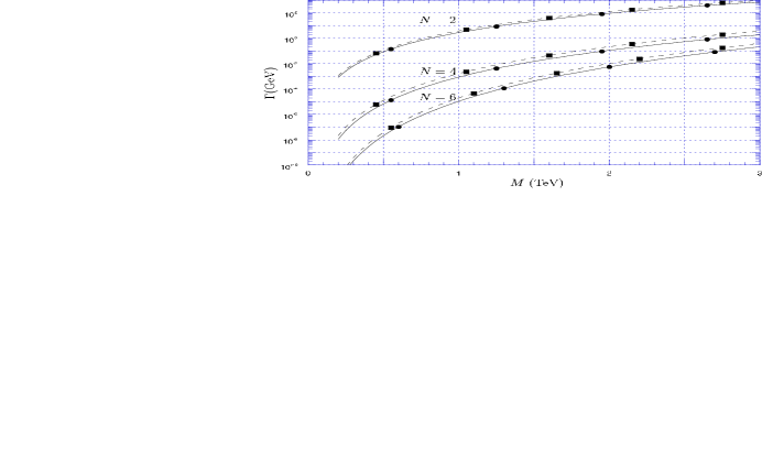
Figure 4: The decays of the $q_{1}^{\bullet}$ or $q_{1}^{\circ}$ (solid) and $g_{1}^{\star}$ (dashed) into SM fields via graviton emission (spin $2$ and scalar combined) are shown as a function of the compactification scale $\mu=M=1/R$ for $M_{D}=5$ TeV. The pairs of curves correspond to $2$, $4$, and $6$ extra dimensions from top to bottom, respectively.

The decay widths of the $q_{1}^{\bullet}$ (or $q_{1}^{\circ}$) and $g_{1}^{\star}$, integrated over the density of graviton states with the form factor as in the prescription of Eq. 33, are illustrated in Fig. 4. The distributions of the graviton mass and missing energy (graviton energy) in the rest frame of the decaying particle are shown in Fig. 5. It is interesting to note that, in this scenario, when gravity propagates in two extra-dimensions ($N=2$), the decays of KK quark or gluon excitations will be mediated mostly by very light gravitons, while for $N\geq 3$ the heavy graviton (mass of order $\mu$) contribution will dominate (see the top of Fig. 5). As a consequence, for $N=2$ the missing energy distribution will have a peak at half the KK excitation mass, while with increasing $N$ the distribution will shift toward larger values. Note also that all of these decays will occur within the detectors in the range of parameter space that we will explore and is depicted here.

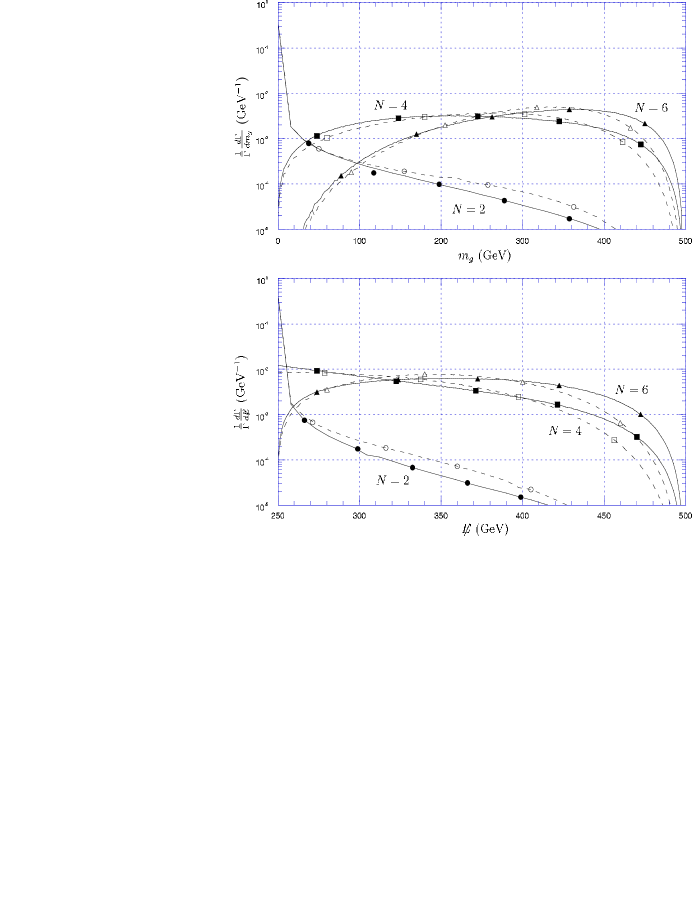
Figure 5: The graviton mass distribution (top) and missing energy distribution (bottom) of the $q_{1}^{\bullet}$ or $q_{1}^{\circ}$ (solid) and $g_{1}^{\star}$ (dashed) are illustrated for $\mu=500$ GeV and $M_{D}=5TeV$. The pairs of curves correspond to $2$, $4$, and $6$ extra dimensions.

The collider signature for the production and decay of gluon or light quark (except the top) KK excitations in this model is SM dijet production with missing energy carried off by the gravitons. This production rate is related to the cross sections for the stable case and the differential branching fractions of the decaying KK states via:

$$d\sigma_{\mathit{tot}}=\sum_{A,B}d\sigma_{prod}(p\bar{p}\rightarrow A\ B)\ \frac{d\Gamma_{A}}{\Gamma_{A}}\ \frac{d\Gamma_{B}}{\Gamma_{B}}.$$ (37)

The sum is over the KK intermediate states, denoted by $A$ and $B$. The spin correlations are not taken into account. The top case will be discussed separately.

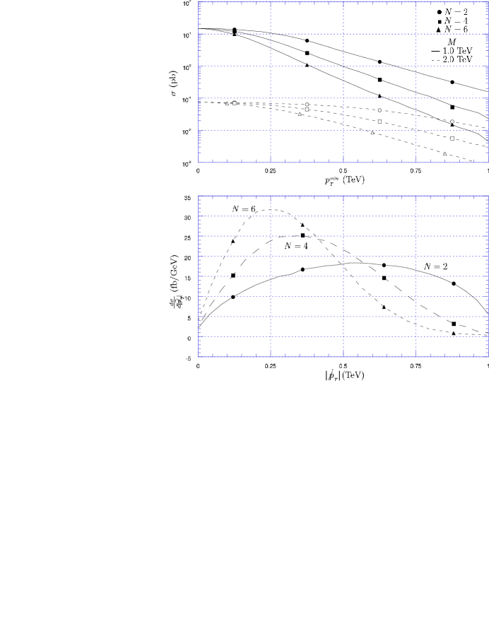
Figure 6: The total cross section for the dijet production plus missing energy from decaying KK final states (top) and the missing transverse momentum $\!\mid\!\!\vec{\not{p}}_{{}_{T}}\!\!\mid\!$ distribution (bottom) are shown for $2$, $4$, and $6$ extra dimensions. The compactification scale is $1$ TeV in the bottom figure, while $1$ and $2$ TeV are shown in the top figure. No cuts are implemented in these graphs, such that the total area under each curve is equal in the bottom graph. (However, all cuts are implemented in the following figures.)

We consider the following two distributions of experimental interest in Fig. 6: the two-jets + missing energy cross-section as a function of the minimum transverse momentum, $p_{{}_{T}}^{{}_{\mathit{min}}}$, of the jets (top), and the cross-section as a function of the missing transverse momentum, $\!\mid\!\!\vec{\not{p}}_{{}_{T}}\!\!\mid\!$ (bottom). The dependence of these distributions on the number of extra dimensions in which gravity propagates (or on the decay mechanism) is encoded in the mass distributions of the gravitons which mediate this decay. For example, if the quark (or gluon) KK excitations decay mostly to light gravitons, the distributions will look like the curves corresponding to $N=2$ in Fig. 6. Conversely, in the case when the KK particles decay to heavy gravitons, these will take almost all available momentum, leaving very little for the two observable jets. Hence, the cross section drops faster with increasing minimum transverse momentum, $p_{{}_{T}}^{{}_{\mathit{min}}}$, and the missing transverse momentum, $\!\mid\!\!\vec{\not{p}}_{{}_{T}}\!\!\mid\!$, distribution shifts toward zero with the increase in $N$. Signals for decays mediated by a different mechanism will fit somewhere among these curves, depending on what fraction of the decays favor light versus heavy gravitons.

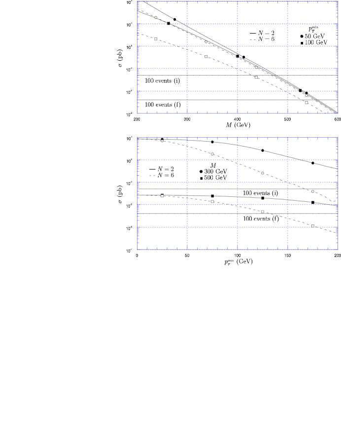
Figure 7: The total cross section for the dijet production plus missing energy from decaying KK final states at the Tevatron Run II energy is illustrated as a function of $\mu$ for fixed $p_{{}_{T}}^{{}_{\mathit{min}}}$ (top) and as a function of the minimum transverse momentum $p_{{}_{T}}^{{}_{\mathit{min}}}$ for fixed values of the compactification scale $\mu$ (bottom). Solid horizontal lines mark $100$ events at the initial and final projected luminosities. In this and the following figures, we implement cuts on the $p_{{}_{T}}$, rapidity, and separation of the jets.

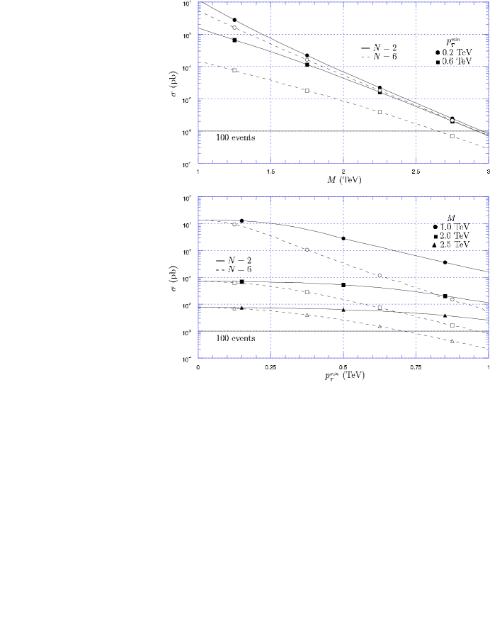
Figure 8: The same as Fig. 7, but for the LHC. The solid horizontal line marks $100$ annual events at the projected luminosity.

The dependence of the cross section on the mass of the KK excitations for different $p_{{}_{T}}$ cuts is shown in Fig. 7 for the Tevatron Run II and Fig. 8 for the LHC. For illustration, the values of $N=2$ and $N=6$ for the number of extra dimensions have been used. Note that the case $N=6$ is the least favorable to direct observation, since the heavier the graviton mass, the lower the transverse momentum of the quark or gluon jets will be. Beside the cuts specified in the figure, we also require that the rapidity be limited to the range $\mid\!y\!\mid\,\leq 2.5$, and the two observable jets be separated by a cone of radius larger than $R=\sqrt{(\Delta\phi)^{2}+(\Delta\eta)^{2}}=0.4$, where $\phi$ is the azimuthal angle and $\eta$ is the pseudorapidity, which is related to the polar angle $\theta$ via $\eta=-\ln\tan(\theta/2)$. Requiring for direct observation at least $100$ events with $p_{{}_{T}}>50$ GeV at Tevatron and $p_{{}_{T}}>400$ GeV at LHC, respectively, we see that the Tevatron reach extends to about $550$ GeV, while at LHC KK excitations can be discovered in this model for values of the compactification scale as high as $3$ TeV. We assume here that cuts on missing transverse momentum (Fig. 9) are used to greatly reduce the SM background.

Figure 9: The missing transverse momentum distribution is illustrated for Run II of the Tevatron (top) and the LHC (bottom). The three curves represent $2$, $4$, and $6$ extra dimensions. By $\!\mid\!\!\vec{\not{p}}_{{}_{T}}\!\!\mid\!$ we denote the vectorial sum of the transverse momentum of the two emitted gravitons (which is equal and opposite to that of the quarks). The compactification scale and minimum transverse momentum are $400$ GeV and $50$ GeV for the Tevatron and $1$ TeV and $200$ GeV for the LHC, respectively.

We present here some comments on the SM background. There are many SM processes which can give rise to a dijet signal with missing energy. Some examples include $WZ,\ ZZ,\ q\bar{q}Z$ and $t\bar{t}$ production, where neutrinos arising from $Z$ and $W$, for example, carry off the mising energy; also $2\rightarrow 2$ QCD processes with missing energy due to the mismeasurement of jet energies. Of course, cuts on the minimum $p_{T}$ of the jets and on the missing transverse energy can be implemented to greatly improve the signal-to-background ratio. A complete analysis of SM backgrounds (including the optimization of cuts) is beyond the purpose of this paper. However, for illustration, we consider the specific cuts in Table II. For example, for $p_{T}^{min}=600$ GeV and $|\vec{\not{p}}_{T}|>1200$GeV at the LHC, the SM background has been evaluated in Ref. [27] to be $\sim 40$ events for $10^{5}$ pb^-1 luminosity, while the signal would be 600, 2000, and 50 events for $N=2$ and compactification scale $M=1,2,$ and 3 TeV respectively. For $N=6$, the signal would be 30, 130 and 10 events, for the same values of $M$. We see that the signal is larger than or comparable with the background in almost all of these cases ($N=6,M=3$ TeV is borderline). Moreover, these cuts can be optimized in order to enhance the signal-to-background ratio. For example, in the case of $M=1$ TeV, the 1200 GeV cut on the missing transverse energy is too hard (this is why so few events remain), and by relaxing it the signal can be increased substantially.

Finally, we consider the production and decay of KK excitations of the top quark. As seen from Fig. 2, the cross-section for this process is less than $1\%$ than the total KK excitation production cross-section. However, if the mass of first KK tower is smaller than about $1$ TeV, there will be of order $10^{4}$ KK top pair events produced at LHC. Unlike the other KK excitations, the $t^{\bullet}$ can also decay to $W^{+\star}b$. For $\mu<1$ TeV, the decay to $W^{+\star}b$ is dominant (unless $N=2$; in this case, we need $\mu<0.4$ TeV). Furthermore, the $W^{+\star}$ can decay either into $W$ + graviton, in which case the signal for this process will be $b\bar{b}W^{+}W^{-}$ in the final state, plus missing energy; or into $d^{\bullet}u$, for example, in which case the signal could be two $b$ jets plus four light quark jets plus missing energy.

The results discussed thus far apply to the case when the first KK excitations of quarks and gluons have nearly the same masses. This is true at tree level; however, radiative corrections can lift this mass degeneracy [22]. In this situation, the decays of the first KK excitations can proceed through cascades to the lightest KK particle (LKP). For example, if the LKP is the $\gamma^{\star}$ (as in [22]), the $g_{n}^{\star}$ can decay through $g_{n}^{\star}\rightarrow q\bar{q}_{n}^{\bullet}\rightarrow q\bar{q}\gamma^{\star}$. The case when the LKP is stable has been analyzed in Ref. [28] and the collider phenomenology has been found to be very similar to that of supersymmetry with an almost degenerate spectrum. Here we want to comment on the possibility that the LKP decays through a gravity mediated mechanism, as discussed above in this section. In this case, the collider signal will be an excess of two photon events instead of two jets (or two leptons, if the LKP is an $l^{\bullet}$, for example). Moreover, since the momenta of the SM particles radiated in the process of cascade decays to the LKP (the two quarks in the $g_{n}^{\star}$ decay example above) should be rather small (of the order of the mass splitting between the different KK excitations), the momentum of the LKP wil be nearly the same as the momentum of the KK particle initiating the decay (the $q_{n}^{\bullet}$ or $g_{n}^{\star}$). Then the $p_{T}$ and missing energy distrinutions of the two photon (or two lepton) events will be the same as the distributions computed above for the dijet case. We leave a more complete analysis (including branching fractions for gravity mediated decays versus cascade decays to the LKP) to a future paper [29].

		Signal (evts.)
$p_{T}^{cut}$	Background	$M=1$ TeV		$M=2$ TeV		$M=3$ TeV
(GeV)	(evts.)	$N=2$	$N=6$	$N=2$	$N=6$	$N=2$	$N=6$
100	$3\times 10^{6}$	$1\times 10^{6}$	$9\times 10^{5}$	$7\times 10^{3}$	$6\times 10^{3}$	$84$	$80$
200	$2\times 10^{5}$	$9\times 10^{5}$	$2\times 10^{5}$	$6\times 10^{3}$	$4\times 10^{3}$	$80$	$65$
300	$9\times 10^{3}$	$4\times 10^{5}$	$4\times 10^{4}$	$5\times 10^{3}$	$3\times 10^{3}$	$73$	$50$
400	$1\times 10^{3}$	$1\times 10^{5}$	$2\times 10^{3}$	$4\times 10^{3}$	$1\times 10^{3}$	$65$	$34$
500	$2\times 10^{2}$	$5\times 10^{4}$	$2\times 10^{2}$	$3\times 10^{3}$	$4\times 10^{2}$	$58$	$20$
600	$4\times 10\$	$6\times 10^{2}$	$3\times 10\$	$2\times 10^{3}$	$1\times 10^{2}$	$50$	$10$

Table 2: SM background and UED signals with $p_{T}>p_{T}^{cut},\ \not{E_{T}}>2p_{T}^{cut}$ (for $10^{5}\hbox{pb}^{-1}$ at LHC).

6. Conclusions

In this work, we have investigated in detail the phenomenology of the UED model, which is a class a class of string-inspired models in which all of the SM fields can propagate into one TeV-scale extra dimension. Specifically, we calculated the effects that the KK excitations of the quarks and gluons have on multijet final states at high energy hadronic colliders including the LHC and Tevatron Runs I and II. We performed these calculations for the case where the lowest-lying KK excitations of the light quarks and gluons are stable, as well as the case where they decay within the detector. For the decaying scenario, we examined a scenario in the context of a fat brane that may provide enough KK number violation to accommodate lifetimes that would be consistent with cosmological observations without resulting in a significant production rate for single KK final states. We presented a detailed evaluation for the fat brane scenario, and also illustrated the dependence of our results on the decay structure.

Our results for proton-proton collisions at the Tevatron Run I place the mass bound for the first excited KK states at $350$–$400$ GeV. For the Run II energies, the mass bound can be raised to $450$–$550$ GeV. Proton-antiproton collisions at the LHC energy can probe much further: UED KK excitations will either be discovered or the mass limit will be raised to about $3$ TeV. If the UED compactification scale is less than $1.5$ TeV, then at the LHC energy we might be able to see the first two KK excitations of the quarks and gluons, thereby uniquely establishing the extra-dimensional nature of the new physics.

The signatures of the production of UED KK excitations will be vastly different for short-lived and long-lived states. Stable, slowly moving KK quarks produced at colliders will hadronize, resulting in tracks with high ionization. The production of numerous heavy, charged stable particles will produce a clear signal of new physics. They will appear as a heavy replica of the light SM quarks, with both up- and down-type quark charges, but with two KK quarks corresponding to each SM quark. The two towers, $q_{n}^{\bullet}$and $q_{n}^{\circ}$, will be polarized with opposite chirality for all cross-channel processes due to $Z_{2}$ parity conservation. If the KK excitations of the light quarks and gluons are short-lived, then the signal will be SM dijet production with missing energy carried off by the emitted gravitons. This missing energy significantly reduces the SM background. The production of the lowest-lying KK excitations of the gluons and light quarks gives rise to only dijets plus missing energy (due to the escaping gravitons), and no multijet signals (at order $\alpha_{S}^{2}$). Such final states will distinguish this new physics from supersymmetry, which will produce multijet final states in addition to dijets.

Acknowledgments

We are grateful to X. Tata for useful discussions. This work was supported in part by the U.S. Department of Energy Grant Numbers DE-FG03-98ER41076 and DE-FG02-01ER45684.

Appendix

We begin with the UED $5$D Lagrangian density. The procedure for obtaining the effective $4$D theory is to Fourier expand the $5$D fields in terms of the extra dimension $y$, and then integrate over $y$. Here, we will begin by obtaining the mass contributions to the KK excitations from their kinetic terms as well as their interactions with the Higgs potential. We will then proceed to derive the complete set of interactions between the KK excitations of the quarks and gluons. We will not discuss purely gluonic interactions, which were described elaborately in Ref. [12].

Each of the $5$D multiplets $Q(x,y)$, $U(x,y)$, and $D(x,y)$ can be Fourier expanded in terms of the compactified dimension $y$, restricted in an $S_{1}/Z_{2}$ orbifold, as

$$Q(x,y) \!\!\!= \!\!\!\frac{1}{\sqrt{\pi R}}\left\{\left(\!\begin{array}[]{c}u(x)\\ d(x)\end{array}\!\right)_{\!L}+\sqrt{2}\sum_{n=1}^{\infty}\left[Q_{L}^{n}(x)\cos\left(\frac{ny}{R}\right)+Q_{R}^{n}(x)\sin\left(\frac{ny}{R}\right)\right]\right\}$$ (40)

$$U(x,y) \!\!\!= \!\!\!\frac{1}{\sqrt{\pi R}}\left\{u_{R}(x)+\sqrt{2}\sum_{n=1}^{\infty}\left[U_{R}^{n}(x)\cos\left(\frac{ny}{R}\right)+U_{L}^{n}(x)\sin\left(\frac{ny}{R}\right)\right]\right\}$$ (41)

$$D(x,y) \!\!\!= \!\!\!\frac{1}{\sqrt{\pi R}}\left\{d_{R}(x)+\sqrt{2}\sum_{n=1}^{\infty}\left[D_{R}^{n}(x)\cos\left(\frac{ny}{R}\right)+D_{L}^{n}(x)\sin\left(\frac{ny}{R}\right)\right]\right\}\,,$$ (42)

where $Q_{L,R}^{n}(x)\equiv\frac{1}{2}(1\mp\gamma_{5})q_{n}^{\bullet}(x)$ as in Eq. 11 and $\gamma_{5}$ is the usual $4$D Dirac matrix. Note that the decomposition in Eq.’s 40–42 gives the correct SM zero mode chiral structure for the fermions. Similarly, the gluon field $A_{M}(x,y)$ can be Fourier expanded as:

$$A_{\mu}^{a}(x,y)=\frac{1}{\sqrt{\pi R}}\left[A_{\mu 0}^{a}(x)+\sqrt{2}\sum_{n=1}^{\infty}A_{\mu,n}^{a}(x)\cos(\frac{ny}{R})\right]$$ (43)

$$A_{4}^{a}(x,y)=\frac{\sqrt{2}}{\sqrt{\pi R}}\sum_{n=1}^{\infty}A_{4,n}^{a}(x)\sin(\frac{ny}{R})\,.$$ (44)

Under the transformation $y\rightarrow-y$, the decomposed gluon fields transform as $A_{\mu}^{a}(x,-y)=A_{\mu}^{a}(x,y)$ and $A_{4}^{a}(x,-y)=-A_{4}^{a}(x,y)$. Notice that $Z_{2}$ parity and KK number are conserved in the interactions involving the gauge fields and fermions. We choose to work in the unitary gauge, where we can apply the gauge choice $A_{4,n}^{a}(x)=0$ [18].

The primary contribution to the KK masses stems from the kinetic term in the Lagrangian density:

$$\mathcal{L}_{5}=i\bar{Q}(x,y)\left\{\Gamma^{M}\left[\partial_{M}+ig_{{}_{5}}T^{a}A_{M}^{a}(x,y)\right]\right\}Q(x,y)\,.$$ (45)

There are similar terms for the other $5$D multiplets. Here, $g_{{}_{5}}$ is the $5$D strong coupling and $M$ is the $5$D analog of the Lorentz index $\mu$, i.e., $M\in\{\mu,4\}$. Integration of the kinetic terms in Eq. (45) over the compactified dimension $y$ results in:

$$i\!\!\int_{\mbox{\raisebox{-3.91806pt}{\scriptsize{$\!\!\!\!0$}}}}^{\mbox{\raisebox{2.71246pt}{\scriptsize{$\!\!\!\!\pi R$}}}} \!\!\!\!\!\!\!\!\bar{Q}(x,y) \!\!\!\!\Gamma^{M}\partial_{M}Q(x,y)dy=i\left[(\bar{u}(x)\bar{d}(x))_{L}\gamma^{\mu}\partial_{\mu}\left(\!\begin{array}[]{c}u(x)\\ d(x)\end{array}\!\right)_{\!L}\right.$$ (48)

$$\!\!\!+ \!\!\!\!\!\!\!\sum_{n=1}^{\infty}\left.\bar{Q}_{L}^{n}(x)\gamma^{\mu}\partial_{\mu}Q_{L}^{n}(x)+\bar{Q}_{R}^{n}(x)\gamma^{\mu}\partial_{\mu}Q_{R}^{n}(x)\right.$$

$$\!\!\!+ \!\!\!\!\!\!\!\left.i\frac{n}{R}\bar{Q}_{L}^{n}(x)Q_{R}^{n}(x)+i\frac{n}{R}\bar{Q}_{R}^{n}(x)Q_{L}^{n}(x)\right]\,.$$

There are similar expressions for the $U(x,y)$ and $D(x,y)$ multiplets. The mass of the KK excitations are identified as $n\mu$, where $\mu$ is the compactification scale ($\mu=1/R$). Thus, in the absence of the Higgs mechanism, the KK excitations have masses given by $M_{n}=n/R=n\mu$. The corresponding mass matrix is:

$$(\bar{Q}^{n}(x),\bar{U}^{n}(x))\left(\begin{array}[]{cr}\frac{n}{R}&0\\ 0&-\frac{n}{R}\end{array}\right)\left(\!\begin{array}[]{c}Q^{n}(x)\\ U^{n}(x)\end{array}\!\right)\,,$$

where $Q^{n}(x)$ represents the upper component of the doublet, with charge $2/3$. Note that there is no mixing between the different KK levels, i.e., between $Q^{n}(x)$ and $Q^{m}(x)$ for $n\neq m$.

Additional mass contributions arise from the Yukawa couplings of the $5$D quark multiplets via the Higgs VEV’s:

$$\!\!\!\!i \!\!\!\!\int_{\mbox{\raisebox{-3.91806pt}{\scriptsize{$\!\!\!\!0$}}}}^{\mbox{\raisebox{2.71246pt}{\scriptsize{$\!\!\!\!\pi R$}}}}\left[\lambda_{u}^{5}\bar{Q}(x,y)i\sigma_{2}H^{\ast}(x,y)U(x,y)+\lambda^{5}_{d}\bar{Q}(x,y)H(x,y)D(x,y)+h.c.\right]dy=$$

$$\!\!\!\!i \!\!\!\!\left\{M_{u}\left[\bar{u}(x)u(x)+\sum_{n=1}^{\infty}\left[\bar{Q}_{L}^{n}(x)U_{R}^{n}(x)+\bar{Q}_{R}^{n}(x)U_{L}^{n}(x)\right]\right]\right.$$

$$\!\!\!\!+ \!\!\!\!\left.\lambda_{u}\left[\bar{u}(x)u(x)h(x)+\sum_{n=1}^{\infty}\left[\bar{Q}_{L}^{n}(x)U_{R}^{n}(x)+\bar{Q}_{R}^{n}(x)U_{L}^{n}(x)\right]h(x)\right]+\lambda_{d}\textnormal{terms}\right\}\,,$$

where $\lambda_{u}\equiv\lambda_{u}^{5}/\sqrt{\pi R}$ and $M_{u}\equiv\lambda_{u}\!\!<\!\!H\!\!>$. The $(Q^{n}(x),U^{n}(x))$ mass matrix, including these Yukawa contributions as well as the kinetic terms, is:

$$(\bar{Q}^{n}(x),\bar{U}^{n}(x))\left(\begin{array}[]{cr}\frac{n}{R}&M_{u}\\ M_{u}&-\frac{n}{R}\end{array}\right)\left(\!\begin{array}[]{c}Q^{n}(x)\\ U^{n}(x)\end{array}\!\right)\,.$$

The eigenvalues of the this mass matrix give the net mass $M_{n}$ of the KK modes in terms of the mass of the corresponding quark field $M_{q}$ and the mass from the compactification $n/R$:

$$M_{n}=\sqrt{\frac{n^{2}}{R^{2}}+M_{q}^{2}}\,.$$ (51)

We redefine the $U^{n}(x)$ field by $U^{n}(x)\rightarrow\gamma_{5}U^{n}(x)$. In our subsequent calculations, we neglect the SM quark masses except for the top mass $M_{t}$.

The interactions between the $5$D $Q(x,y)$ fields and the $5$D gluon fields $A_{M}^{a}(x,y)$ are given by:

$$- \!\!\!\!\!g_{{}_{5}} \!\!\!\!\!\!\int_{\mbox{\raisebox{-3.91806pt}{\scriptsize{$\!\!\!\!0$}}}}^{\mbox{\raisebox{2.71246pt}{\scriptsize{$\!\!\!\!\pi R$}}}}\bar{Q}(x,y)\Gamma^{M}T^{a}A_{M}^{a}(x,y)Q(x,y)dy$$

$$=- \!\!\!\!\!\!\!g \!\!\!\!\!\left.\mbox{\raisebox{-2.15277pt}{\Huge$\{$}}\bar{q}_{L}(x)\gamma^{\mu}T^{a}q_{L}(x)A_{\mu,0}^{a}(x)+\sum_{n=1}^{\infty}\left[\bar{Q}_{L}^{n}(x)\gamma^{\mu}T^{a}Q_{L}^{n}(x)+\bar{Q}_{R}^{n}\gamma^{\mu}T^{a}Q_{R}^{n}(x)\right]A_{\mu,0}^{a}(x)\right.$$

$$\!\!\!+ \!\!\!\sum_{n=1}^{\infty}\left[\bar{q}_{L}(x)\gamma^{\mu}T^{a}Q_{L}^{n}(x)+\bar{Q}_{L}^{n}(x)\gamma^{\mu}T^{a}q_{L}(x)\right]A_{\mu,n}^{a}(x)$$

$$\!\!\!+ \!\!\!\frac{1}{\sqrt{2}}\sum_{n,m,\ell=1}^{\infty}\left.\left[\bar{Q}_{L}^{n}(x)\gamma^{\mu}T^{a}Q_{L}^{m}(x)(\delta_{\ell,\mid m-n\mid}+\delta_{\ell,m+n})\right.\right.$$

$$\!\!\!+ \!\!\!\left.\left.\bar{Q}_{R}^{n}(x)\gamma^{\mu}T^{a}Q_{R}^{m}(x)(\delta_{\ell,\mid m-n\mid}-\delta_{\ell,m+n})\right]A_{\mu,\ell}^{a}\mbox{\raisebox{-2.15277pt}{\Huge$\}$}}\right.\,,$$

where $g\equiv g_{{}_{5}}/\sqrt{\pi R}$. There are similar interactions involving the $U$ and $D$ fields. In terms of the $q_{n}^{\bullet}$ and $q_{n}^{\circ}$ fields (Eq. 11), the interactions are:

$$\mathcal{L}_{\mathit{int}}= \!\!\!- \!\!\!\!\!g\mbox{\raisebox{-2.15277pt}{\Huge$\{$}}\!\!\left.\bar{q}(x)\gamma^{\mu}T^{a}q(x)A_{\mu,0}^{a}(x)+\sum_{n=1}^{\infty}\left[\bar{q}_{n}^{\bullet}(x)\gamma^{\mu}T^{a}q_{n}^{\bullet}(x)+q_{n}^{\circ}(x)\gamma^{\mu}T^{a}\bar{q}_{n}^{\circ}(x)\right]A_{\mu,0}^{a}(x)\right.$$

$$\!\!\!+ \!\!\!\sum_{n=1}^{\infty}\left[\bar{q}_{L}(x)\gamma^{\mu}T^{a}q_{n}^{\bullet}(x)+\bar{q}_{n}^{\bullet}(x)\gamma^{\mu}T^{a}q_{L}(x)\right]A{}_{\nu,n}^{a}(x)$$

$$\!\!\!+ \!\!\!\sum_{n=1}^{\infty}\left[\bar{q}_{R}(x)\gamma^{\mu}T^{a}q_{n}^{\circ}(x)+\bar{q}_{n}^{\circ}(x)\gamma^{\mu}T^{a}q_{R}(x)\right]A{}_{\nu,n}^{a}(x)$$

$$\!\!\!+ \!\!\!\frac{1}{\sqrt{2}}\sum_{n,m,\ell=1}^{\infty}\left[-\bar{q}_{n}^{\bullet}(x)\gamma^{\mu}\gamma_{5}T^{a}q_{m}^{\bullet}(x)+\bar{q}_{n}^{\circ}(x)\gamma^{\mu}\gamma_{5}T^{a}q_{m}^{\circ}(x)\right]A_{\mu,\ell}^{a}\,\delta_{\ell,m+n}$$

$$\!\!\!+ \!\!\!\frac{1}{\sqrt{2}}\sum_{n,m,\ell=1}^{\infty}\left.\left[\bar{q}_{n}^{\bullet}(x)\gamma^{\mu}T^{a}q_{m}^{\bullet}(x)+\bar{q}_{n}^{\circ}(x)\gamma^{\mu}T^{a}q_{m}^{\circ}(x)\right]A_{\mu,\ell}^{a}\,\delta_{\ell,\mid m-n\mid}\right.\!\!\mbox{\raisebox{-2.15277pt}{\Huge$\}$}}\,.$$

The relative coupling strengths are summarized in Fig. 1.

References

- [1] N. Arkani-Hamed, S. Dimopoulos and G. Dvali, Phys. Lett. B 429, 263 (1998); Phys. Rev. D59, 086004 (1999); I. Antoniadis, N. Arkani-Hamed, S. Dimopoulos and G. Dvali, Phys. Lett. B 436, 257 (1998).
- [2] E. Witten, Nucl. Phys. B 471, 135 (1996); J. Lykken, Phys. Rev. D 54, 3693 (1996).
- [3] See, for example: E.A. Mirabelli, M. Perelstein, and M.E. Peskin, Phys. Rev. Lett. 82, 2236 (1999); G.F. Giudice, R. Rattazzi, and J.D. Wells, Nucl. Phys. B 554, 3 (1999); J.E. Hewett, Phys. Rev. Lett. 82, 4765 (1999); G. Shiu and S.H.H. Tye, Phys. Rev. D58, 106007 (1998); T. Banks, A. Nelson, and M. Dine, J. High Energy Phys. 06, 014 (1999); P. Mathews, S. Raychaudhuri, and S. Sridhar, Phys. Lett. B450, 343 (1999) and J. high Energy Phys. 07, 008 (2000); T.G. Rizzo, Phys. Rev. D 59, 115010 (1999); C. Balazs, H.-J. He, W.W. Repko, C.-P. Yan, and D.A. Dicus, Phys. Rev. Lett. 83, 2112 (1999); I. Antoniadis, K. Benakli, and M. Quirós, Phys. Lett. B 360, 176 (1999); P. Nath, Y. Yamada, and M. Yamaguchi, ibid. 466, 100 (1999); W.J. Marciano, Phys. Rev. D 60, 09006 (1999); T. Han, D. Rainwater, and D. Zepenfield, Phys. Lett. B 463, 93 (1999); K. Aghase and N.G. Deshpande, ibid. 456, 60 (1999); G. Shiu, R. Shrock, and S.H.H. Tye, ibid. 458, 274 (1999); K. Cheung and Y. Keung, Phys. Rev. D 60, 112003 (1999); K.Y. Lee, S.C. Park, H.S. Song, J.H. Song and C.H. Yu, Phys. Rev. D 61, 074005 (2000); hep-ph/0105326.
- [4] T. Han, J. D. Lykken and R. J. Zhang, Phys. Rev. D 59, 105006 (1999).
- [5] J. Lykken and S. Nandi, Phys. Lett. B 485, 224 (2000).
- [6] V. Barger, T. Han, C. Kao and R.J. Zhang, Phys. Lett. B 461, 34 (1999); S. Cullen and M. Perelstein, Phys. Rev. Lett. 83, 268, 1999; L.J. Hall and D. Smith, Phys. Rev. D 60, 085008 (1999); S.C. Kappadath et. al., Bull. Am. Astron. Soc. 30 926 (1998); Ph.D. Thesis, available at http://wwwgro.sr.unh.edu/users/ckappada/ckappada.html; D.A. Dicus, W.W. Repko and V.L. Teplitz, Phys. Rev. D 62, 076007 (2000). M. Biesiada and B. Malec, ibid. 65, 043008; K.A. Milton, R. Kantowski, C. Kao and Y. Wang, Mod. Phys. Lett. A 16, 2281 (2001); S. Hannestad, G. Raffelt, Phys. Rev. Lett. 87, 051301 (2001); M. Fairbarin, J. High Energy Phys. 02, 024 (2002).
- [7] I. Antoniadis, Phys. Lett. B 246 377 (1990).
- [8] E. Accomando, I. Antoniadis, and K. Benakli, Nucl. Phys. B 579, 3 (2000); A. Datta, P.J. O’Donnell, Z.H. Lin, X. Zhang, and T. Huang, Phys. Lett. B 483, 203 (2000).
- [9] T.G. Rizzo and J.D. Wells, Phys. Rev. D 61, 016007 (2000) ; C.D. Carone, Phys. Rev. D 61 015008, 2000.
- [10] M. Masip and A. Pomarol, Phys. Rev. B 60, 096005 (1999); P. Nath, Y. Yamada and M. Yamaguchi, Phys. Lett. B 466, 100 (1999).
- [11] C.D. McMullen and S. Nandi, hep-ph/0110275.
- [12] D.A. Dicus, C.D. McMullen and S. Nandi, Phys. Rev. D 65, 076007 (2002).
- [13] T. Appelquist, H.-C. Cheng and B.A. Dobrescu, Phys. Rev. D 64, 035002 (2001).
- [14] A. DeRujula, A. Donini, M.B. Gavela and S. Rigolin, Phys. Lett. B 482, 195 (2000).
- [15] T.G. Rizzo, Phys. Rev. D 64, 095010 (2001).
- [16] T. Appelquist and B.A. Dobrescu, Phys. Lett. B 516, 85 (2001); K. Agashe, N.G. Deshpande and G.H. Wu, Phys. Lett. B 514, 309 (2001).
- [17] A. Delgado, A. Pomarol and M. Quirós, Phys. Rev. D 60, 095008 (1999); J. High Energy Phys. 01, 030 (2000); A. Pomarol and M. Quirós, Phys. Lett. B 438, 255 (1998); E. Dudas, Class. Quantum Grav. 17, R41 (2001); M. Masip and A. Pomarol, Phys. Rev. D 60, 096005 (1999).
- [18] K.R. Dienes, E. Dudas, and T. Ghergetta, Nucl. Phys. B 537, 47 (1999); J. Papavassiliou and A. Santamaria Phys. Rev. D 63, 125014 (2001).
- [19] J.A.M. Vermaseren, math-ph/0010025.
- [20] R.S. Chivukula, D.A. Dicus and H.-J. He, Phys. Lett. B 525, 175 (2002).
- [21] J.M. Cornwall, D.N. Levin and G. Tiktopoulos, Phys. Rev. Lett. 30, 1268 (1973); Phys. Rev. D 10, 1145 (1974); D.A. Dicus and V.S. Mathur, Phys. Rev. D 7, 3111 (1973); B.W.Lee, C. Quigg and H.B.Thacker, Phys. Rev. Lett. 38, 883 (1977); Phys. Rev. D 16, 1519 (1977); M. J. G. Veltman, Acta Phys. Polon. B 8, 475 (1977); C.H. Llewellyn Smith, Phys. Lett. B 46, 233 (1973).
- [22] H. C. Cheng, K. T. Matchev and M. Schmaltz, Phys. Rev. D 66, 036005 (2002).
- [23] K.P. Dienes, E. Dudas and T. Gherghetta, Phys. Lett. B436, 55 (1998); Nucl. Phys. B537, 47 (1999); T. Taylor and G Veneziano, Phys. Lett. B212 147 (1988); D. Ghilencia and G.G. Ross, Phys. Lett. B442 165 (1998); hep-ph/9908369; C. Carone, Phys. Lett. B454 70 (1999); P. H. Frampton and A. Rasin, Phys. Lett. B460, 313 (1999); A. Delgado and M. Quirós, Nucl. Phys. B559, 235 (1999); A. Perez-Lorenzana and R. N. Mohapatra, Nucl. Phys. B559, 255 (1999); Z. Kakushadze and T. R. Taylor, Nucl. Phys. B562, 78 (1999); D. Dumitru and S. Nandi, Phys. Rev. D 62, 046006 (2000); K. Huitu and T. Kobayashi, Phys. Lett. B470, 90 (1999); H. Cheng, B. A. Dobrescu and C. T. Hill, Nucl. Phys. B573, 597 (2000).
- [24] M. Masip, Phys. Rev. D 62, 105012 (2000).
- [25] H.L. Lai et al., Phys. Rev. D 51, 4763 (2000).
- [26] A. Connolly [CDF collaboration], ”Search for long-lived charged massive particles at CDF,” Talk at the American Physical Society (APS) Meeting of the Division of Particles and Fields (DPF ), Los Angeles, CA, Jan -, , hep-ex/9904010.
- [27] S. I. Bityukov and N. V. Krasnikov, Phys. Lett. B 469, 149 (1999).
- [28] H.C. Cheng, K.T. Matchev and M. Schmaltz, Phys. Rev. D 66, 056006 (2002).
- [29] C. Macesanu, C.D. McMullen and S. Nandi, Phys. Lett. B 546, 253 (2002).
- [30] J. M. Smillie and B. R. Webber, JHEP 0510, 069 (2005).