Talk at the VIth International School-Seminar “Actual Problems of High Energy Physics” August 7-16, 2001, Gomel, Belarus

Abstract

We present the SIMUB package developed at Dubna for MC generation of $B$ meson production and decays. The starting version of the package includes lepton modes of $B$ decays, in particular, semileptonic decays $B\to D^{(*)}l\nu$ and “golden” mode $B\to J/\psi(\to\mu\mu)\,\phi(\to KK)$ with taking into account all theoretical refinements including $B^{0}-\overline{B}^{0}$ oscillations and angular correlations.

SIMUB is a Monte Carlo (MC) generator of $B$-meson production and decays which is under developing at Dubna for the Compact Muon Solenoid (CMS) Project at CERN (see SIMUB documentation in [1]). The main motivation for this activity was that already existing generators do not take into account the theoretical refinements which are of great importance for MC studies of $B$-decay dynamics. In particular, in the generators PYTHIA [2], QQ [3], and EvtGen [4], the time-dependent spin-angular correlations between the final-state particles are not included in the proper way for the so called “golden” decay $B^{0}_{s}(t),\overline{B}^{0}_{s}(t)\to J/\Psi(\to\mu^{+}\mu^{-})\,\phi(\to K^{+}K^{-})$. The dynamics of this decay is described by four-dimension probability distribution function depending on decay time and three physical angles. The algorithms of multidimensional random number generation have been elaborated and then implemented in the package SIMUB to provide tools for MC simulation of sequential two-body decays $B^{0}(t)\,,\overline{B}^{0}(t)\to a(\to a_{1}a_{2})\,b(\to b_{1}b_{2})$ in accordance with theoretical time-dependent angular distributions.

This paper is organized as follows. First, some general theoretical aspects are considered in the context of $B^{0}-\overline{B}^{0}$ oscilations and angular correlations. Then, we discuss the algorithms of multidimensional random number generation restricting ourself by detail consideration of only $B\to V_{1}(\to\mu^{+}\mu^{-})\,V_{2}(\to P^{+}P^{-})$ channel and its $B^{0}_{s}\to J/\psi\phi$ “golden” mode. Finally, we present a general information about SIMUB package and compare time and angular distributions for “golden” decay mode generated by SIMUB with those obtained by using PYTHIA.

1. $B^{0}-\overline{B}^{0}$ mixing and time evolution of neutral
          $B$-meson states

The time dependence of $B^{0}\to f$ decays, in which $f$ is not a CP eigenstate, is not purely exponent due to the presence of $B^{0}-\overline{B}^{0}$ mixing. This mixing arises due to either mass difference or decay-width difference between the mass eigenstates of the $B^{0}-\overline{B}^{0}$ system. The time evolution of the state $|B^{0}(t)\rangle$ ($|\overline{B}^{0}(t)\rangle$) of initially, i.e. at time $t=0$, present $B^{0}$ ($\overline{B}^{0}$) meson can be described as follows:

$$|B^{0}(t)\rangle=g_{+}(t)|B^{0}\rangle+g_{-}(t)|\overline{B}^{0}\rangle\,,\qquad g_{+}(t=0)=1\,,\quad g_{-}(t=0)=0\,;$$

$$|\overline{B}^{0}(t)\rangle=\bar{g}_{+}(t)|B^{0}\rangle+\bar{g}_{-}(t)|\overline{B}^{0}\rangle\,,\qquad\bar{g}_{+}(t=0)=0\,,\quad\bar{g}_{-}(t=0)=1\,.$$

The strong eigenstates $|B^{0}(t)\rangle$ and $|\overline{B}^{0}(t)\rangle$ are not eigenstates of the full Hamiltonian due to the weak interaction. Thus, they most generally evolve according to the Schroedinger equation:

$$i\frac{\partial}{\partial t}\left(\begin{array}[]{c}|B^{0}(t)\rangle\\ |\overline{B}^{0}(t)\rangle\end{array}\right)=\bigg{(}{\bf M}-\frac{i}{2}{\bf\Gamma}\bigg{)}\left(\begin{array}[]{c}|B^{0}(t)\rangle\\ |\overline{B}^{0}(t)\rangle\end{array}\right)\,,$$

$${\bf M}=\left(\begin{array}[]{cc}M_{11}&M_{12}\\ M_{21}&M_{22}\end{array}\right)\,,\quad{\bf\Gamma}=\left(\begin{array}[]{cc}\Gamma_{11}&\Gamma_{12}\\ \Gamma_{21}&\Gamma_{22}\end{array}\right)\,.$$

Diagonalization of full Hamiltonian ${\bf M}-(i/2){\bf\Gamma}$ (see [5] for more detail) gives

$$g_{+}(t)=\frac{1}{2}\Big{(}e^{-i\mu_{+}t}+e^{-i\mu_{-}t}\Big{)}\,,\quad g_{-}(t)=\frac{\alpha}{2}\Big{(}e^{-i\mu_{+}t}-e^{-i\mu_{-}t}\Big{)}\,;$$

$$\bar{g}_{+}(t)=g_{-}(t)/\alpha^{2}\,,\qquad\qquad\quad~{}\bar{g}_{-}(t)=g_{+}(t)\,.$$

Here $\mu_{\pm}\equiv M_{L/H}-(i/2)\Gamma_{L/H}$ are eigenvalues of the full Hamiltonian corresponding to the masses and total widths of physical “light” and “heavy” eigenstates of full Hamiltonian $|B_{L/H}\rangle\equiv|B_{\pm}\rangle$, and

$$\alpha=\sqrt{\frac{M^{*}_{12}-\Gamma^{*}_{12}}{M_{12}-\Gamma_{12}}}\approx\sqrt{\frac{M^{*}_{12}}{M_{12}}}=\eta^{B}_{CP}$$ (3)

is a phase factor defining CP transformation of flavor eigenstates of neutral $B$-meson system: $CP|B^{0}(t)\rangle=\eta^{B}_{CP}|\overline{B}^{0}(t)\rangle$.

In Eq. (3) we have made a good approximation $\Gamma_{12}\ll M_{12}$ valid for $B^{0}-\overline{B}^{0}$ system. This approximation implies that there is no $CP$ violation in $B^{0}-\overline{B}^{0}$ mixing, i.e. the probability for $B^{0}$ to oscillate to a $\overline{B}^{0}$ is equal to the probability of a $\overline{B}^{0}$ to oscillate to a $B^{0}$:

$$\mbox{Prob}(\overline{B}^{0}\to B^{0})\approx\mbox{Prob}(B^{0}\to\overline{B}^{0}).$$

Such an asymmetry in mixing, which results from $|\alpha|\not=1$, is often reffered to as indirect CP violation. The situation with indirect $CP$-violation in $B^{0}-\overline{B}^{0}$ mixing is in contrast to the $K^{0}-\overline{K}^{0}$ system, in which

$$\mbox{Prob}(\overline{K}^{0}\to K^{0})>\mbox{Prob}(K^{0}\to\overline{K}^{0}).$$

The indirect $CP$-violation is the main source of $CP$-violation in neutral $K$ decays.

From $CPT$ theorem it follows that

$$M_{11}=M_{22}\equiv M\,,\qquad M_{12}=M_{21}^{*}\,;$$

$$\Gamma_{11}=\Gamma_{22}\equiv\Gamma\,,\qquad\quad~{}\Gamma_{12}=\Gamma_{21}^{*}\,,$$

where $M$ and $\Gamma$ are ”mean” values: $M=(M_{L}+M_{H})/2$, $\Gamma=(\Gamma_{L}+\Gamma_{H})/2$. The values $\Delta M=(M_{H}-M_{L})$ and $\Delta\Gamma=(\Gamma_{H}-\Gamma_{L})$ are used also.

The explicit expressions for mixing probabilities as a function of time are given by

$$\mbox{Prob}(B^{0}~{}\mbox{at}~{}t|B^{0}~{}\mbox{at}~{}t=0) = \mbox{Prob}(\overline{B}^{0}~{}\mbox{at}~{}t|\overline{B}^{0}~{}\mbox{at}~{}t=0)$$

$$= \frac{1}{4}\Big{[}e^{-\Gamma_{L}t}+e^{-\Gamma_{H}t}+2e^{-\Gamma t}\mbox{cos}(\Delta Mt)\Big{]}\,,$$

$$\mbox{Prob}(\overline{B}^{0}~{}\mbox{at}~{}t|B^{0}~{}\mbox{at}~{}t=0) = \frac{1}{4}|\alpha|^{2}\Big{[}e^{-\Gamma_{L}t}+e^{-\Gamma_{H}t}-2e^{-\Gamma t}\mbox{cos}(\Delta Mt)\Big{]}\,,$$

$$\mbox{Prob}(B^{0}~{}\mbox{at}~{}t|\overline{B}^{0}~{}\mbox{at}~{}t=0) = \frac{1}{4|\alpha|^{2}}\Big{[}e^{-\Gamma_{L}t}+e^{-\Gamma_{H}t}-2e^{-\Gamma t}\mbox{cos}(\Delta Mt)\Big{]}\,,$$

For case $|\alpha|=1$ (no indirect CP violation) in approximation $\Gamma_{L}\approx\Gamma_{H}$, the latter two expressions in Eqs. (LABEL:mix-prob) can be rewritten in form

$$\mbox{Prob}(\overline{B}^{0}~{}\mbox{at}~{}t|B^{0}~{}\mbox{at}~{}t=0)=\mbox{Prob}(B^{0}~{}\mbox{at}~{}t|\overline{B}^{0}~{}\mbox{at}~{}t=0)\approx\mbox{sin}^{2}\left(\frac{\Delta Mt}{2}\right)$$

which coincides with the formula for $B^{0}-\overline{B}^{0}$ mixing probability used in PYTHIA [2]:

$${\cal P}_{flip}=\mbox{sin}^{2}\left(\frac{xt}{2\langle\tau\rangle}\right)\,.$$ (5)

Here $\langle\tau\rangle=1/\Gamma$ is the mean lifetime, and $x$ is the mixing parameter [6]:

$$x=x_{d}=\Delta M/\Gamma=0.74\pm 0.02 B^{0}_{d}-\overline{B}^{0}_{d}~{}\mbox{system;}$$ in

$$x=x_{s}=\Delta M/\Gamma>19 B^{0}_{s}-\overline{B}^{0}_{s}~{}\mbox{system.}$$ in

In PYTHIA, the initial $B^{0}$ meson is allowed with the probability (5) to decay like a $\overline{B}^{0}$ and vice versa.

2. Time evolution of decay amplitudes

Time evolution of the amplitudes of transitions $|B^{0}(t)\rangle,\overline{B}^{0}(t)\rangle\to|f\rangle$ induced by Hamiltonian $H_{eff}$ is represented by

$$A_{f}(t)\equiv\langle f|{\cal H}_{eff}|B^{0}(t)\rangle=g_{+}(t)\langle f|{\cal H}_{eff}|B^{0}\rangle+g_{-}(t)\langle f|{\cal H}_{eff}|\overline{B}^{0}\rangle\,,\qquad$$

$$\bar{A}_{f}(t)\equiv\langle f|{\cal H}_{eff}|\overline{B}^{0}(t)\rangle=\bar{g}_{+}(t)\langle f|{\cal H}_{eff}|B^{0}\rangle+\bar{g}_{-}(t)\langle f|{\cal H}_{eff}|\overline{B}^{0}\rangle\,.\qquad$$ (6)

If $|f\rangle$ is the eigenstate of $CP$-operator

$$CP|f\rangle=\eta_{CP}^{f}|f\rangle\,,\quad(\eta_{CP}^{f}=\pm 1)\,,$$

the relations (6) can be rewritten in form

$$A_{f}(t)=\langle f|{\cal H}_{eff}|B^{0}\rangle\bigg{[}g_{+}(t)+g_{-}(t)\frac{1}{\eta_{CP}^{f}\eta_{CP}^{B}}\xi_{f}\bigg{]}\,,$$

$$\bar{A}_{f}(t)=\langle f|{\cal H}_{eff}|B^{0}\rangle\bigg{[}\bar{g}_{+}(t)+\bar{g}_{-}(t)\frac{1}{\eta_{CP}^{f}\eta_{CP}^{B}}\xi_{f}\bigg{]}\,.$$

Here

$$\xi_{f}\equiv\frac{\langle f|{\cal H}_{eff}|\bar{B}^{0}\rangle}{\langle f|{\cal H}_{eff}^{CP}|\bar{B}^{0}\rangle}=|\xi_{f}|e^{-i\phi_{f}}\,,$$

where ${\cal H}_{eff}^{CP}\equiv CP{\cal H}_{eff}CP$, and $\phi_{f}$ is the CP-violating weak phase [7].

The CP-violating weak phase $\phi_{f}$ is introduced through interference effects between $B^{0}-\overline{B}^{0}$ mixing and decay process with final state $|f\rangle$ being the eigenstate of $CP$ operator. In case of decays $B^{0}_{q},\overline{B}^{0}_{q}\to f$, where $q\in{d,s}$, the value of weak phase $\xi^{(q)}_{f}$ can be expressed in terms of matrix elements of the combinations ${\cal Q}^{jq}$ of four-quark operators and Wilson coefficients involved in the low energy effective Hamiltonian $H_{eff}$ (see Refs. [7, 8]):

$$\xi^{(q)}_{f}=e^{-i\phi_{mix}^{q}}\frac{\sum_{j=u,c}\lambda_{j}^{(q)}\langle f|{\cal Q}^{jq}|\overline{B}_{q}^{0}\rangle}{\sum_{j=u,c}\lambda_{j}^{(q)*}\langle f|{\cal Q}^{jq}|\overline{B}_{q}^{0}\rangle}\,.$$ (7)

Here $\phi_{mix}^{q}$ is the $B_{q}^{0}-\bar{B}_{q}^{0}$ mixing phase:

$$\phi_{mix}^{q}\equiv 2\mbox{arg}(V_{tq}^{*}V_{tb})=\left\{\begin{array}[]{ll}~{}~{}2\beta&\mbox{for $q=d$}\,,\\ -2\delta\gamma&\mbox{for $q=s$}\,,\\ \end{array}\right.$$

where $V_{ij}$ is the Cabibbo-Kobayashi-Maskawa (CKM) matrix elements while $\beta$ and $\delta\gamma$ are standard parameters related with angles of the unitary triangles.

In general, the observable $\xi_{f}^{(q)}$ suffers from large theoretical uncertainties in the hadronic matrix elements $\langle f|{\cal Q}^{jq}|\overline{B}_{q}^{0}\rangle$. However, if the decays $B^{0}_{q},\overline{B}^{0}_{q}\to f$ are dominated by a single CKM amplitude, the corresponding matrix elements in Eq. (7) are canceled, and $\xi_{f}^{(q)}$ takes the simple form:

$$\xi_{f}^{(q)}=e^{-i\phi_{j}^{(q)}}\,,\quad\phi_{j}^{(q)}=2[\mbox{arg}(V_{tq}^{*}V_{tb})-\mbox{arg}(V_{jq}^{*}V_{jb})]=\phi_{mix}^{q}-\phi^{j}_{dec}$$

where $q\in d,s$, $j\in u,c$, and $\phi^{j}_{dec}$ is a $CP$-violating weak decay phase:

$$\phi_{dec}^{j}\equiv 2\mbox{arg}(V_{jq}^{*}V_{jb})=\left\{\begin{array}[]{ll}-2\gamma&\mbox{for $j=u$ -- dominant $b\to u\bar{u}q$ }\,,\\ ~{}~{}~{}~{}0&\mbox{for $j=c$ -- dominant $b\to c\bar{c}q$ }\,,\\ \end{array}\right.$$

where $\gamma$ is the angle of unitary triangle.

3. Transversity amplitudes and time-dependent
          observables for decays $B(t)\to V_{1}V_{2}$

The decay $B^{0}(t)\to V_{1}V_{2}$, where $V_{1}$ and $V_{2}$ are vector mesons in final state, is described in terms of three transverse amplitudes $A_{0}$, $A_{||}$ and $A_{\bot}$ [9]:

$$A(B^{0}(t)\to V_{1}V_{2})=A_{0}(t)\frac{m_{V_{2}}}{E_{V_{2}}}\epsilon^{*L}_{V_{1}}\epsilon^{*L}_{V_{2}}-A_{||}(t)\frac{1}{\sqrt{2}}\vec{\epsilon}^{\,*T}_{V_{1}}\vec{\epsilon}^{\,*T}_{V_{2}}-A_{\bot}(t)\frac{i}{\sqrt{2}}\vec{\epsilon}^{\,*}_{V_{1}}\vec{\epsilon}^{\,*}_{V_{2}}\hat{\vec{p}}\,.$$ (8)

Here $E_{V_{2}}$ is the energy of the $V_{2}$ in the $V_{1}$ rest frame; $\hat{\vec{p}}$ is a unit vector in the direction of the momentum of $V_{2}$ in $V_{1}$ rest frame; $\vec{\epsilon}_{V_{1}}$ and $\vec{\epsilon}_{V_{2}}$ are the polarization three-vectors in the $V_{2}$ rest frame; $\epsilon^{L}\equiv\hat{\vec{p}}\cdot\vec{\epsilon}$ is the longitudinal component and $\vec{\epsilon}^{\,T}$ is the transverse component of the polarization vector. The decay $\overline{B}^{0}(t)\to V_{1}V_{2}$ is described in analogous way in terms of the transversity amplitudes $\bar{A}_{0}$, $\bar{A}_{||}$ and $\bar{A}_{\bot}$.

Eq. (8) corresponds to decomposition of final state of $B^{0}(t)\to V_{1}V_{2}$ decay over transversity basis which can be represented in form of 3-dimensional vector

$$|f\rangle=(|(V_{1}V_{2})_{0}\rangle,|(V_{1}V_{2})_{||}\rangle,|(V_{1}V_{2})_{\bot}\rangle)\,.$$

The transversity components are eigenstates of $CP$-operator:

$$CP|(V_{1}V_{2})_{f}\rangle=\eta_{CP}^{f}|(V_{1}V_{2})_{f}\rangle\,,\quad(f=0,||,\bot)\vspace*{-4mm}$$

with eigenvalues

$$\eta_{CP}^{0}=1\,,\quad\eta_{CP}^{||}=1\,,\quad\eta_{CP}^{\bot}=-1\,.\vspace*{-2mm}$$

Thus, the Eq. (S0.Ex27) with $\langle f|{\cal H}_{eff}|B^{0}\rangle\equiv A_{f}(0)$ can be applied to calculate the time evolution of transversity amplitudes $A_{f}(t)$ ($f=0,||,\bot$).

Matrix element squared involves into consideration the following six time-dependent bilinear combinations of transversity amplitudes (observables):

$${\cal O}_{1}(t)=|A_{0}(t)|^{2}\,,\quad{\cal O}_{2}(t)=|A_{||}(t)|^{2}\,,\quad{\cal O}_{3}(t)=|A_{\bot}(t)|^{2}\,,$$

$${\cal O}_{4}(t)=\mbox{Im}\Big{(}A_{||}^{*}(t)A_{\bot}(t)\Big{)}\,,\quad{\cal O}_{5}(t)=\mbox{Re}\Big{(}A_{0}^{*}(t)A_{||}(t)\Big{)}\,,\quad$$

$${\cal O}_{6}(t)=\mbox{Im}\Big{(}A_{0}^{*}(t)A_{\bot}(t)\Big{)}\,,\vspace*{-2mm}$$ (9)

in case of decays $B^{0}(t)\to V_{1}V_{2}$, and similar combinations of $\bar{A}_{f}(t)$ ($f=0,||,\bot$) for decays $\overline{B}^{0}(t)\to V_{1}V_{2}$.

4. The time-dependent angular distributions

Let us consider sequential two-body decays

$$B^{0}(t)\,,\overline{B}^{0}(t)\to a(\to a_{1}a_{2})\,b(\to b_{1}b_{2})\,,\vspace*{-2mm}$$

where $a$ and $b$ are vector mesons decaying into pairs of particles $a_{1}$, $a_{2}$ and $b_{1}$, $b_{2}$, respectively. The angular distributions for these decays are governed by spin-angular correlations (see [10]-[12]) and involve three physical angles. In case of the so-called helicity frame [11] these angles are defined as shown in Fig. (1). The $z$-axis is defined to be the direction of $b$-particle in the rest frame of the $B^{0}$. The $x$-axis is defined as any arbitrary fixed direction in the plane normal to the $z$-axis. The $y$-axis is then fixed uniquely via $y=x\times z$. The angles ($\Theta_{a_{1}}$, $\chi_{a_{1}}$) specify the direction of the $a_{1}$ in the $a$ rest frame while ($\Theta_{b_{1}}$, $\chi_{b_{1}}$) are the direction of $b_{1}$ in the $b$ rest frame. Since the orientation of $x$-axis is a matter of convention, only the difference $\chi=\chi_{a_{1}}-\chi_{b_{1}}$ of the two azimuthal angles is physical.

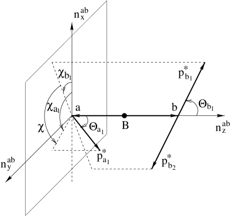
Figure 1: The decay $B\to a(\to a_{1}a_{2})\,b(\to b_{1}b_{2})$ in helicity frame

In most general form the angular distribution for decay $B^{0}(t)\to a(\to a_{1}a_{2})\,b(\to b_{1}b_{2})$ can be expressed as

$$f_{0}(\Theta_{a_{1}},\Theta_{b_{1}},\chi;t)\equiv\frac{d^{3}\Gamma}{d\mbox{cos}\Theta_{a_{1}}d\mbox{cos}\Theta_{b_{1}}d\chi}=\frac{9}{64\pi}\,\sum^{6}_{i=1}{\cal O}_{i}(t)g_{i}(\Theta_{a_{1}},\Theta_{b_{1}},\chi)\,,$$ (10)

where ${\cal O}_{i}$ ($i=1,...,6$) are the observables (9) and $g_{i}$ are the functions of physical angles $\Theta_{a_{1}}$, $\Theta_{b_{1}}$ and $\chi$.

The time-dependent angular distribution function (10) is used as density of the probability function for MC simulation of the vertex and kinematics of the final-state particles in case of decay $B^{0}(t)\to a(\to a_{1}a_{2})\,b(\to b_{1}b_{2})$. The variables of the function $f_{0}(\Theta_{a_{1}},\Theta_{b_{1}},\chi;t)$ can not be factorized and randomly generated in the independent way. Nevertheless, the random generation of $\mbox{cos}\,\Theta_{a_{1}}$, $\mbox{cos}\,\Theta_{b_{1}}$, $\chi$ and $t$ can be performed either simultaneously according to distribution function (10) by using four-dimensional random generator or successively, one after another, by using single-dimensional random number generators with accordance to distribution functions obtained by successive integration of the function (10) over its variables.

Let as consider the latter approach in the case of sequential random generation of the variables $t$, $\chi$, $\mbox{cos}\,\Theta_{a_{1}}$ and $\mbox{cos}\,\Theta_{b_{1}}$. The following three distribution function are used in this case:

$$f_{1}(\Theta_{a_{1}},\chi;t)\equiv\int_{-1}^{+1}d\mbox{cos}\Theta_{b_{1}}\,f_{0}(\Theta_{a_{1}},\Theta_{b_{1}},\chi;t)\,,$$

$$f_{2}(\chi;t)\equiv\int_{-1}^{+1}d\mbox{cos}\Theta_{a_{1}}\,f_{1}(\Theta_{a_{1}},\chi;t)\,,$$ (11)

and

$$f_{3}(t)\equiv\int_{0}^{2\pi}d\chi f_{2}(\chi;t)\,={\cal O}_{1}(t)+{\cal O}_{2}(t)+{\cal O}_{3}(t)\,.$$ (12)

The procedure is as follows:

• First, the proper time $t$ is randomly generated according to the distribution function $f_{3}(t)$.

• Second, the angle $\chi$ is randomly generated according to the single-dimensional distribution given by function $f_{2}(\chi;t)$ with $t$ being fixed to be equal to the time, generated at the first step.

• Then, the value $\mbox{cos}\,\Theta_{a_{1}}$ is generated according to distribution function $f_{1}(\Theta_{a_{1}},\chi;t)$ with values of $t$ and $\chi$ fixed to be equal to their values generated at the previous two steps.

• Finally, the value of $\mbox{cos}\,\Theta_{b_{1}}$ can be generated according to the single-dimensional distribution given by function $f_{0}(\Theta_{a_{1}},\Theta_{b_{1}},\chi;t)$ with a properly fixed values of $t$, $\chi$ and $\mbox{cos}\,\Theta_{a_{1}}$.

The functions of Eqs. (11) and (12) present the most important experimentally observable distributions.

5. Decays $B^{0}(t)\,,\bar{B}^{0}(t)\to V_{1}(l^{+}l^{-})V_{2}(P^{+}P^{-})$

In case of sequential decays $B^{0}(t)\,,\overline{B}^{0}(t)\to V_{1}(\to l^{+}l^{-})V_{2}(\to P^{+}P^{-})$, where $l^{\pm}$ and $P^{\pm}$ are lepton and pseudoscalar mesons, respectively, let associate the particles in the final states with general notations used in Fig. 1 as follows:

$$V_{1}\to a\,,\quad l^{+}\to a_{1}\,,\quad l^{-}\to a_{2}\,,$$

$$V_{2}\to b\,,\quad P\to b_{1}\,,\quad P^{\prime}\to b_{2}\,.$$

In this case the functions $g_{i}(\Theta_{a_{1}},\Theta_{b_{1}},\chi)$ in Eq. (10) are defined as [11]:

$$g_{1}=4\mbox{sin}^{2}\Theta_{a_{1}}\mbox{cos}^{2}\Theta_{b_{1}}\,,$$

$$g_{2}=(1+\mbox{cos}^{2}\Theta_{a_{1}})\mbox{sin}^{2}\Theta_{b_{1}}-\mbox{sin}^{2}\Theta_{a_{1}}\mbox{sin}^{2}\Theta_{b_{1}}\mbox{cos}2\chi\,,$$

$$g_{3}=(1+\mbox{cos}^{2}\Theta_{a_{1}})\mbox{sin}^{2}\Theta_{b_{1}}+\mbox{sin}^{2}\Theta_{a_{1}}\mbox{sin}^{2}\Theta_{b_{1}}\mbox{cos}2\chi\,,$$

$$g_{4}=2\mbox{sin}^{2}\Theta_{a_{1}}\mbox{sin}^{2}\Theta_{b_{1}}\mbox{sin}2\chi\,,$$

$$g_{5}=-\sqrt{2}\mbox{sin}2\Theta_{a_{1}}\mbox{sin}2\Theta_{b_{1}}\mbox{cos}\chi\,,$$

$$g_{6}=\sqrt{2}\mbox{sin}2\Theta_{a_{1}}\mbox{sin}2\Theta_{b_{1}}\mbox{sin}\chi\,.$$ (13)

The explicit form of the distribution functions (11) are given below:

$$f_{1}(\mbox{cos}\Theta_{a_{1}},\chi;t) = ~{}~{}\frac{4}{3}{\cal O}_{1}(t)\,\mbox{sin}^{2}\Theta_{a_{1}}+\frac{4}{3}{\cal O}_{2}(t)\,(1-\mbox{sin}^{2}\Theta_{a_{1}}\mbox{cos}^{2}\chi)$$

$$+\frac{4}{3}{\cal O}_{3}(t)\,(1-\mbox{sin}^{2}\Theta_{a_{1}}\mbox{sin}^{2}\chi)-{\cal O}_{4}(t)\,\mbox{sin}^{2}\Theta_{a_{1}}\mbox{sin}2\chi\,,$$

$$f_{2}(\chi,t) = ~{}~{}{\cal O}_{1}(t)+\frac{1}{2}{\cal O}_{2}(t)\,(3-2\mbox{cos}^{2}\chi)$$ (14)

$$+\frac{1}{2}{\cal O}_{3}(t)\,(3-2\mbox{sin}^{2}\chi)-{\cal O}_{4}(t)\,\mbox{sin}2\chi\,.$$

6. Physics parameters for decay $B^{0}_{s}\to J/\psi\phi$

For numerical MC simulation of the decay $B^{0}_{s}\to J/\psi\phi$ the following physics parameters should be defined:

• $\alpha=1$ – no CP violation in $B^{0}-\overline{B}^{0}$-mixing;

• $M_{L}=5.3696$ GeV – mass of the “light” $B$ meson;

• $\Delta M=M_{H}-M_{L}=$ 10.6 ps^-1;

• $\Gamma_{L}=1/\tau$ – width of the “light” $B$ meson, where $\tau=1.493$ ps;

• $\Delta\Gamma=\Gamma_{H}-\Gamma_{L}=0.2\Gamma_{L}$;

• $\phi_{j}^{(s)}=0.03\div 0.06$ – CP-violating weak phase;

• initial values of observables at time $t=0$: $|A_{0}(0)|$, $|A_{||}(0)|$, $|A_{\bot}(0)|$, and two CP-conserving strong phases $\delta_{1}\equiv\mbox{arg}[A_{||}^{*}(0)A_{\bot}(0)]$ and $\delta_{2}\equiv\mbox{arg}[A_{0}^{*}(0)A_{\bot}(0)]$.

The time-reversal invariance and naive factorization lead to the following common property:

$$\mbox{Im}[A_{0}^{*}(0)A_{\bot}(0)]=0\,,\quad\mbox{Im}[A_{||}^{*}(0)A_{\bot}(0)]=0\,,$$

$$\mbox{Re}[A_{0}^{*}(0)A_{||}(0)]=\pm|A_{0}(0)A_{||}(0)|\,.$$

Moreover, in absence of strong final-state interactions, $\delta_{1}=\pi$ and $\delta_{2}=0$.

Using low-energy effective Hamiltonian [8] for nonleptonic $b$-quark transitions $b\to s\bar{c}c$, the amplitudes $A_{f}(0)$ ($f=0,||,\bot$) of $B^{0}_{s}\to J/\psi\,\phi$ decay can be calculated within the framework of naive factorization in terms of the form factors of transitions $B\to\phi$ induced by quark currents. The $B\to\phi$ form factors can be related to the $B\to K^{*}$ case by using SU(3) flavor symmetry. In table 1 we collect the predictions of Ref. [13] for the ratios of $B^{0}_{s}\to J/\psi\,\phi$ observables calculated with $B\to K^{*}$ form factors given by different models [14]–[16]. The quantity

$$\frac{\Gamma_{0}(0)}{\Gamma_{0}(0)+\Gamma_{T}(0)}=\frac{|A_{0}(0)|^{2}}{|A_{0}(0)|^{2}+|A_{||}(0)|^{2}+|A_{\bot}(0)|^{2}}$$

describes the ratio of the longitudinal to the total rate at $t=0$.

Table 1. Predictions for $B^{0}_{s}\to J/\psi\,\phi$ observables

7. General structure of program SIMUB

The package for generation of production of $B$-mesons and their decays, SIMUB, is kept under the directory SIMUB_V_X (X is the version number) which has the following main parts:

• bb_gen – routines needed to generate $b\bar{b}$ events (FORTRAN, PYTHIA, HBOOK);

• bb_frg – routines performing string fragmentation and generation of $B$-mesons (FORTRAN, PYTHIA, HBOOK). The program is a part of BB_dec program but may be used as independent program;

• BB_dec – routines performing $B$-decays (C++, FORTRAN, PYTHIA, HBOOK, ROOT) and storing the results into standard HEPEVT-format Ntuple for further usage in the CMS detector simulation or in format JETSET for analysis;

• include – a collection of common blocks for bb_gen, bb_frg and BB_dec.

To simulate the $B$-meson production in $pp$ collisions with PYTHIA [2] (programs bb_gen and bb_frg) we used the modified routines from the FORTRAN-based package described in [17].

The data flow between three main parts (bb_gen, bb_frg, and BB_dec) of the package SIMUB_V_X is organized in the following two steps:

• At the first step the $b\bar{b}$-events are generated by the program bb_gen and written to Ntuple bb_X_YYY.

• At the next step the program BB_dec reads $b\bar{b}$-events from Ntuple bb_X_YYY and performs the string fragmentation (via call bb_frg) and decay of $B$ mesons. The decay modes and mechanisms are defined by user. The full information about $B$ decay events is stored in Ntuple BB_dec.ntpl. Its format (HEPEVT or JETSET) is defined by user.

8. Inheritance of classes in the program BB_dec

The example of class inheritance of BB_dec program is shown in Fig. 2 for the case of time-depended decay channel

$$B^{0}(t)\,,\overline{B}^{0}(t)\to V_{1}(\to l^{+}l^{-})\,V_{2}(\to P^{+}P^{-})\,,\vspace*{-2mm}$$

where $V_{1}$ and $V_{2}$ are the vector particles, $l^{+}$ and $l^{-}$ are the leptons, $P^{+}$ and $P^{-}$ are the pseudoscalar mesons. The thick and thin arrows show the directions of class inheritance from mother to daughter classes. Thick arrows correspond to main inheritance ways. The name of each class coincides with the name of subdirectory where this class is kept. The upper dashed-line box corresponds to the directory src. The lower dashed-line boxes unite the names of classes which are in the same subdirectory at the same level. In case when several classes belong to the same subdirectory, its name coincides with the name of the class where the thick incoming arrow shows to. The directories are included one into another in the directions opposite to thick arrows.

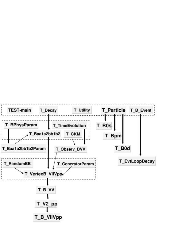
Figure 2: The class inheritance of the BB_dec program in case of simulation of decays $B^{0}(t)\,,\overline{B}^{0}(t)\to V_{1}(\to\l^{+}\l^{-})V_{2}(\to P^{+}P^{-})$

The main directory src, shown in Fig. 2 as upper dashed-line box, contains five subdirectories T_Decay, T_Particle, T_B_Event, T_Utility and TEST-main. The subdirectory T_Decay contains definition of the mother class with the same name as well as subdirectories with classes which are common for different decay channels. The subdirectory T_Particle contains the definition of the mother class with the same name and subdirectories with daughter classes T_B0s, T_Bpm and T_B0d which define the properties and decay modes for $B^{0}_{d}$ ($\overline{B}^{0}_{d}$), $B^{\pm}$ and $B^{0}_{s}$ ($\overline{B}^{0}_{s}$) mesons, respectively. The directory T_B_Event contains the definition of the mother class with the same name and daughter class T_EvtLoopBDec with a loop over all events with $B$-mesons. In the loop, each event is read from the ROOT Tree bb_frg.root and, then, the decays of $B$-mesons are performed according to modes defined in the samples of classes T_B0s, T_Bpm and T_B0d both for particles and anti-particles. The directory T_Utility consists of the auxiliary classes and functions. The directory TEST-main contains the main programs for testing of classes.

The directory src also includes the file T_EvtLoopBdec_main.C containing a main() function which is not shown in Fig. 2. In this file, user can find the example of loop over the events.

9. Monte Carlo methods for generation of decays           $B^{0}(t)\to V_{1}(\to\l^{+}\l^{-})\,V_{2}(\to P^{+}P^{-})$

In class T_VertexB_VllVpp, the variables describing the decay channel and MC method for random generation are defined. The member function T_VertexB_VllVpp::DecayB_VllVpp generates four random numbers – proper decay time $t$ and angular variables $\mbox{cos}\,\Theta_{b_{1}}$, $\mbox{cos}\,\Theta_{a_{1}}$ and $\chi$ – according to distribution function given by Eq. (10). Then, DecayB_VllVpp calculates Lorenz vector characterizing the decay vertex in Laboratory system.

Two MC methods of random numbers generation are implemented in the class T_VertexB_VllVpp.

The first method is based on the filling of the large single-dimensional array f4_Integ[n4_cells] of real numbers which represents numerically the four-dimensional distribution function corresponding to $f_{0}(\Theta_{a_{1}},\Theta_{b_{1}},\chi;t)$ given by Eqs. (10) and (13). The array f4_Integ contains ${\tt n4\_cells}={\tt fNpx}\times{\tt fNpy}\times{\tt fNpz}\times{\tt fNpt}$ elements, where the variables fNpx, fNpy, fNpz and fNpt define the MC generator resolutions. The array f4_Integ is filled in the constructor of class T_VertexB_VllVpp where the memory space for the array is reserved during all time of the existence of this class sample. The array f4_Integ is used in the member function T_VertexB_VllVpp::GetRandom4 performing fast generation of the four random values of $\mbox{cos}\,\Theta_{b_{1}}$, $\mbox{cos}\,\Theta_{a_{1}}$, $\chi$ and $t$ .

The second method involves sequential generation of random numbers according to approach which is based on usage of single-dimensional distribution functions given by Eqs. (12) and (14). This method was already described in section 4. In this case the constructor T_VertexB_VllVpp does not fill any arrays and, therefore, it does not reserve the memory and may be used for definition of big number of particles decaying in the same mode.

These methods have been tested in case of MC simulation of the “golden” decay mode $B^{0}_{s}(t),\overline{B}^{0}_{s}(t)\to J/\psi(\to\mu^{+}\mu^{-})\,\phi(\to K^{+}K^{-})$ with values of physics parameters fixed according to section 6. Both methods demonstrated the identical results with suitable time and memory consuming.

The time-dependent angular correlations in the decays of type $B^{0}(t)\to V_{1}(\to\l^{+}\l^{-})\,V_{2}(\to P^{+}P^{-})$ can be used in data analysis to extract CP-violating asymmetries, $B^{0}-\overline{B}^{0}$ mixing parameters and other observables [13, 19, 20]. Therefore, the decay dynamics described by angular correlations (10) should be included without fail into MC generators developed for physics studies.

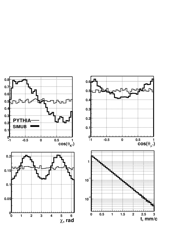
Figure 3: Comparison of time and angular distributions for decay $B^{0}_{s}(t),\overline{B}^{0}_{s}(t)\to J/\psi(\to\mu^{+}\mu^{-})\,\phi(\to K^{+}K^{-})$ generated by SIMUB and PYTHIA. For time $t$ we use units 1mm/$c\approx 3.33\times 10^{-12}$ sec

In Fig. 3 we compare time and angular distributions in the helicity frame for decay $B^{0}_{s}(t),\overline{B}^{0}_{s}(t)\to J/\psi(\to\mu^{+}\mu^{-})\,\phi(\to K^{+}K^{-})$ generated by SIMUB and PYTHIA. The difference between these two generators becomes more clear when slices over time and angular variables are cut from the kinematical phase space. The angular distributions shown in Fig. 3 are built for the following kinematical slices:

$$\chi: 0.01~{}\mbox{mm/}c<t<0.19~{}\mbox{mm/c}\,;$$

$$\mbox{cos}\,\Theta_{\mu^{+}}: 0.01~{}\mbox{mm/}c<t<0.19~{}\mbox{mm/c}\,,\quad 0.3~{}\mbox{rad}<\chi<0.6~{}\mbox{rad}\,;$$

$$\mbox{cos}\,\Theta_{K^{+}}: 0.01~{}\mbox{mm/}c<t<0.19~{}\mbox{mm/c}\,,\quad 0.3~{}\mbox{rad}<\chi<0.6~{}\mbox{rad}\,,$$

$$0.7<\mbox{cos}\,\Theta_{\mu^{+}}<1\,.\vspace*{-4mm}$$

In case of PYTHIA usage, Fig. 3 shows the uniform distributions for angular variables $\mbox{cos}\,\Theta_{b_{1}}$, $\mbox{cos}\,\Theta_{a_{1}}$ and $\chi$ because of lack of time-dependent angular correlations. Due to this simple reason PYTHIA can not be used for MC studies of dynamics of sequential two body decays of $B$ mesons in the channels with intermediate vector mesons. Unfortunately, due to various technical reasons, the both other well known packages, QQ [3] and EvtGen [4], turn out to be also not suitable for study of angular correlations in decays of the type $B\to V_{1}(\mu^{+}\mu^{-})\,V_{2}(P^{+}P^{-})$.

Conclusion

General scheme of program chain and data flow for MC simulation of $B$-meson production and decays have been developed and realized in the package SIMUB which is now in progress. This scheme was tested for case of semileptonic decays $B\to D^{(*)}\mu\nu$ and sequential decays of the type $B\to V_{1}(\to\mu^{+}\mu^{-})\,V_{2}(\to P^{+}P^{-})$. The SIMUB package provides unique tools for MC physics studies of dynamics of semileptonic and ”golden” $B$-decay channels with taking into account $B^{0}-\overline{B}^{0}$ oscillations and angular correlations.

The starting version of the package SIMUB_V_0 is installed and tested at CERN on Linux platform. The package and documentation for user one can find on the SIMUB Home Web Page [1]. There is link to this page from CMS $B$-Physics Group Web Page: http://cmsdoc.cern.ch/~bphys. Now the SIMUB is used within CMS collaboration for exclusive $B$-trigger studies.

References

• [1] http://cmsdoc.cern.ch/~shulga/SIMUB/SIMUB.html
• [2] T. Sjostrand e.a. Computer Physics Commun., 135 (2001) 238.
• [3] http://www.lns.cornell.edu/public/CLEO/soft/QQ/
• [4] http://www.slac.stanford.edu/~lange/EvtGen/
• [5] J.D. Richman, in “Probing the Standard Model of Particle Interactions”, eds. R. Gupta et al., Les Houches, Session LXVIII, 1997, Elservier Science B. V., 1999, Part I, p. 541.
• [6] Particle Data Group, Eur. Phys. J. C15 (2000) p. 1; partial update for the 2002 edition: http://pdg.lbl.gov.
• [7] R. Fleischer and I. Dunietz, Phys. Rev. D55 (1997) p. 259.
• [8] R. Fleischer, Int. J. Mod. Phys. A12 (1997) p. 2459.
• [9] A.S. Dighe et al., Phys. Lett. B369 (1996) p. 144.
• [10] M. Jacob and G.C. Wick, Ann. Phys. 7 (1959) p. 404.
• [11] G. Kramer and W.F. Palmer, Phys. Rev. D45 (1992) p. 193.
• [12] R. Kutschke, see http://www-pat.fnal.gov/personal/kutschke
• [13] A.S. Dighe, I. Dunietz and R. Fleischer, Eur. Phys. J. C6 (1999) p. 647.
• [14] M. Wirbel, B. Stech and M. Bauer, Z. Phys. C29 (1985) p. 637.
M. Bauer, B. Stech and M. Wirbel, Z. Phys. C34 (1987) p. 103.
• [15] J.M. Soares, Phys. Rev. D53 (1996) p. 241.
• [16] H.-Y. Cheng, Z. Phys. C69 (1996) p. 647.
• [17] M. Konecki and A. Starodumov, “$b\bar{b}$ Event Simulation Package User Manual”, CERN, March 16, 1997.
• [18] R. Brun and F. Rademakers, “ROOT. An Object-Oriented Data Analysis Framework”, 2001; http://root.cern.ch.
• [19] G. Valencia, Phys. Rev. D39 (1989) p. 3339.
• [20] I. Dunietz et al., Phys. Rev. D43 (1991) p. 2193.