FTUV-02-0108 ; IFIC-02-10

Generalized Parton Distributions
in Constituent Quark Models$\dagger$

Sergio Scopetta^(a) and Vicente Vento^(b)
(a) Dipartimento di Fisica, Università degli Studi di Perugia, via A. Pascoli 06100 Perugia, Italy
and INFN, sezione di Perugia

(b) Departament de Fisica Teòrica, Universitat de València, 46100 Burjassot (València), Spain
and Institut de Física Corpuscular, Consejo Superior de Investigaciones Científicas
and School of Physics, Korea Institue for Advance Study, Seoul 130-012, Korea

Abstract

An approach is proposed to calculate Generalized Parton Distributions (GPDs) in a Constituent Quark Model (CQM) scenario. These off-diagonal distributions are obtained from momentum space wave functions to be evaluated in a given non relativistic or relativized CQM. The general relations linking the twist-two GPDs to the form factors and to the leading twist quark densities are consistently recovered from our expressions. Results for the leading twist, unpolarized GPD, $H$, in a simple harmonic oscillator model, as well as in the Isgur and Karl model, are shown to have the general behavior found in previous estimates. NLO evolution of the obtained distributions, from the low momentum scale of the model up to the experimental one, is also shown. Further applications of the proposed formalism are addressed.

Pacs: 12.39-x, 13.60.Hb, 13.88+e

Keywords: hadrons, partons, generalized parton distributions, quark models.

sergio.scopetta@pg.infn.it

vicente.vento@uv.es

$\dagger$Supported in part by SEUI-BFM2001-0262 and by MIUR through the funds COFIN01

1 Introduction

In recent years, Generalized Parton Distributions have become one of the main topics of interest in hadronic physics (for recent reviews, see, e.g., [1, 2, 3, 4, 5]). GPDs are a natural bridge between exclusive processes, such as elastic scattering, described in terms of form factors, and inclusive ones, described in terms of structure functions. As it happens for the usual Parton Distributions (PDFs), the measurement of GPDs allows important tests of non-perturbative and perturbative aspects of the theory, QCD, and of phenomenological models of hadrons. Besides, GPDs provide us with a unique way to access several crucial features of the structure of the nucleon. In particular, as pointed out first by Ji [6, 7], by measuring GPDs a test of the Angular Momentum Sum Rule of the proton [8] could be achieved for the first time, determining the quark orbital angular momentum contribution to the proton spin. Therefore, relevant experimental efforts to measure GPDs, by means of exclusive electron Deep Inelastic Scattering (DIS) off the proton, are likely to take place in the next few years [9, 10]. Besides, GPDs measurements will be done soon, also through fitting to the available data of the H1 and ZEUS Collaborations, with the HERMES results used as cross checks but excluded from the fit. In this scenario, it becomes urgent to produce theoretical predictions for the behavior of these quantities. Several calculations have been already performed by using different descriptions of hadron structure: bag models [11, 12], soliton models [3, 13], light-front approaches [14] and phenomenological estimates based on parametrizations of PDFs [15, 16]. Besides, an impressive effort has been devoted to study the perturbative QCD evolution [17, 18] of GPDs, and the GPDs at twist three accuracy[19].

So far, to our knowledge, no calculations have been performed in a Constituent Quark Model (CQM), although a step towards this can be found in [4, 20], where the non relativistic limit is shortly discussed. The CQM has a long story of successful predictions in low energy studies of the electromagnetic structure of the nucleon. In the high energy sector, in order to compare model predictions with data taken in DIS experiments, one has to evolve, according to perturbative QCD, the leading twist component of the physical structure functions obtained at the low momentum scale associated with the model. Such a procedure, already addressed in [21, 22], has proven successful in describing the gross features of standard PDFs by using different CQM (see, e.g., [23]). Similar expectations motivated the present study of GPDs. In this paper, a simple formalism is proposed to calculate the quark contribution to GPDs from any non relativistic or relativized model. By using such a procedure, the GPDs can be easily estimated, providing us with an important tool for the planning of future experiments.

The paper is structured as follows. After the definition of the main quantities of interest, the proposed calculation scheme is introduced in the third section. Then, results obtained in a simple harmonic oscillator model and in the Isgur and Karl model [24] are shown in the following section. NLO perturbative evolution from the scale of the model to the experimental one has been evaluated, and results are presented in the fifth section. Further applications of the procedure, using relativistic models and including antiquarks degrees of freedom, are in progress and will be presented elsewhere [25]. Conclusions are drawn in the last section.

2 General formalism

We adopt the formalism introduced by Ji, who called GPDs “Off-forward parton distributions” in [6, 7]. The connection of these quantities with the “Non diagonal” ones introduced in [2] is discussed in [5, 16] and can be easily obtained.

We are interested in diffractive DIS processes. The absorption of a high-energy virtual photon by a quark in a hadron target is followed by the emission of a particle to be later detected; finally, the interacting quark is reabsorbed back into the recoiling hadron. If the emitted and detected particle is, for example, a real photon, the so called Deeply Virtual Compton Scattering [6, 7] process takes place. Let us think now to a nucleon target, with initial and final momenta $P$ and $P^{\prime}$, respectively. The GPD $H(x,\xi,\Delta^{2})$, the main quantity we deal with in the present paper, is introduced by defining the twist-two part of the light-cone correlation function

$$\int{d\lambda\over 2\pi}e^{i\lambda x}\langle P^{\prime}|\bar{\psi}(-{\lambda n\over 2})\gamma^{\mu}\psi({\lambda n\over 2})|P\rangle =$$

$$=H(x,\xi,\Delta^{2})\bar{U}(P^{\prime})\gamma^{\mu}U(P) + E(x,\xi,\Delta^{2})\bar{U}(P^{\prime}){i\sigma^{\mu\nu}\Delta_{\nu}\over 2M}U(P)+...$$ (1)

where $\Delta=P^{\prime}-P$ is the momentum transfer to the nucleon, ellipses denote higher-twist contributions, $\psi$ is a quark field and M is the nucleon mass. In obtaining Eq. (1), a system of coordinates has been chosen where the photon 4-momentum, $q^{\mu}=(q_{0},\vec{q})$, and $\bar{P}=(P+P^{\prime})^{\mu}/2$ are collinear along $z$. The $\xi$ variable, the so called “skewedness”, parameterizing the asymmetry of the process, is defined by the relation $\xi=-n\cdot\Delta$, where $n=(1,0,0,-1)/(2\Lambda)$ and $\Lambda$ depends on the reference frame, being, for example, $\Lambda=M/2$ in the nucleon rest frame. The $\xi$ variable is bounded by 0 and $\sqrt{-\Delta^{2}}/\sqrt{M^{2}-\Delta^{2}/4}$. Besides, one has $t=\Delta^{2}=\Delta_{0}^{2}-\vec{\Delta}^{2}$.

In the r.h.s of Eq. (1), the dependence of the light-cone correlation function on the GPDs $H(x,\xi,\Delta^{2})$ and $E(x,\xi,\Delta^{2})$ is explicitly shown. By replacing, in the above equation, $\gamma^{\mu}$ with the proper Dirac operator, similar expressions can be derived for defining polarized or chiral odd GPDs [6]. In the following we will only discuss the unpolarized, chiral even, twist-two GPD $H(x,\xi,\Delta^{2})$.
As explained in [6, 7], unlike the usual PDFs, which have the physical meaning of a momentum density in the Infinite Momentum Frame (IMF), GPDs have the meaning of a probability amplitude. They describe the amplitude for finding a quark with momentum fraction $~{}~{}x+\xi/2$ (in the IMF) in a nucleon with momentum $(1+\xi/2)\bar{P}$ and replacing it back into the nucleon with a momentum transfer $\Delta^{\mu}$. Besides, when the quark longitudinal momentum fraction $x$ of the average nucleon momentum $\bar{P}$ is less than $-\xi/2$, GPDs describe antiquarks; when it is larger than $\xi/2$, they describe quarks; when it is between $-\xi/2$ and $\xi/2$, they describe $q\bar{q}$ pairs.

The region $|x|\geq\xi/2$ is often called the DGLAP region, since the $Q^{2}$ evolution of GPDs is governed there by the DGLAP equations of perturbative QCD [26]; the region $|x|\leq\xi/2$ is called the ERBL region, because there the $Q^{2}$ evolution is ERBL-like [27]. One should keep in mind that, besides the variables $x,\xi$ and $\Delta^{2}$ explicitely shown, GPDs depend, as the standard PDFs, on the momentum scale $Q^{2}$ at which they are measured or calculated. For an easy presentation, such a dependence will be omitted in the next two sections of the paper, while it will be properly discussed in the last one.

There are two natural limits for $H(x,\xi,\Delta^{2})$ : i) when $P^{\prime}=P$, i.e., $\Delta^{2}=\xi=0$, the so called “forward” or “diagonal” limit, one recovers the usual PDFs

$$H(x,0,0)=q(x)~{};$$ (2)

ii) the integration over $x$ is independent on $\xi$ and yields the Dirac Form Factor (FF)

$$\int dxH(x,\xi,\Delta^{2})=F_{1}(\Delta^{2})~{}.$$ (3)

Any model estimate of the GPDs has to respect these two crucial constraints.

3 A non relativistic scheme

Our aim now is to evaluate the Impulse Approximation (IA) expression for $H(x,\xi,\Delta^{2})$, suitable to perform CQM calculations.

Let us start from Eq. (1). Substituting the quark fields in the left-hand-side one has

$$\int{d\lambda\over 2\pi}e^{i\lambda x}\langle P^{\prime}|\bar{\psi}(-{\lambda n\over 2})\gamma^{\mu}\psi({\lambda n\over 2})|P\rangle =$$

$$\int{d\lambda\over 2\pi}e^{i\lambda x}\langle P^{\prime}|\sum_{r,r^{\prime},\vec{k}}[d_{r^{\prime}}(\vec{k}+\vec{\Delta})\bar{v}_{r^{\prime}}(\vec{k}+\vec{\Delta})e^{i(k+\Delta)\cdot{\lambda n\over 2}} + b^{+}_{r^{\prime}}(\vec{k}+\vec{\Delta})\bar{u}_{r^{\prime}}(\vec{k}+\vec{\Delta})e^{-i(k+\Delta)\cdot{\lambda n\over 2}}]$$

$$\gamma^{\mu}[b_{r}(\vec{k})u_{r}(\vec{k})e^{-ik\cdot{\lambda n\over 2}} + d^{+}_{r}(\vec{k})v_{r}(\vec{k})e^{ik\cdot{\lambda n\over 2}}]|P\rangle$$

and, taking into account the quarks degrees of freedom only, it becomes

$$C=\sum_{r,r^{\prime},\vec{k}}\int{d\lambda\over 2\pi}e^{i\lambda x}\langle P^{\prime}|\bar{u}_{r^{\prime}}(\vec{k}+\vec{\Delta})b^{+}_{r^{\prime}}(\vec{k}+\vec{\Delta})e^{-i(k+\Delta)\cdot{\lambda n\over 2}}\gamma^{\mu}b_{r}(\vec{k})u_{r}(\vec{k})e^{-ik\cdot{\lambda n\over 2}}|P\rangle~{}.$$

Using IA and integrating over $\lambda$ yields

$$C \simeq \sum_{i}\sum_{r,r^{\prime},\vec{k}}\int{d\lambda\over 2\pi}e^{i\lambda(x-{n\over 2}\cdot(2k+\Delta))}\langle P^{\prime}|\bar{u}_{r^{\prime}}(\vec{k}+\vec{\Delta})b^{+}_{i,r^{\prime}}(\vec{k}+\vec{\Delta})\gamma^{\mu}b_{i,r}(\vec{k})u_{r}(\vec{k})|P\rangle=$$

$$= \sum_{i}\sum_{r,r^{\prime},\vec{k}}\delta\left(x-{n\over 2}\cdot(2k+\Delta)\right)\langle P^{\prime}|\bar{u}_{r^{\prime}}(\vec{k}+\vec{\Delta})b^{+}_{i,r^{\prime}}(\vec{k}+\vec{\Delta})\gamma^{\mu}b_{i,r}(\vec{k})u_{r}(\vec{k})|P\rangle~{}.$$

Let us introduce $\xi=-n\cdot\Delta$, so that Eq. (1) reads now:

$$\sum_{i}\sum_{r,r^{\prime},\vec{k}}\delta\left(x+{\xi\over 2}-n\cdot k\right)\langle P^{\prime}|\bar{u}_{r^{\prime}}(\vec{k}+\vec{\Delta})b^{+}_{i,r^{\prime}}(\vec{k}+\vec{\Delta})\gamma^{\mu}b_{i,r}(\vec{k})u_{r}(\vec{k})|P\rangle=$$ (4)

$$= H(x,\xi,\Delta^{2})\bar{U}(P^{\prime})\gamma^{\mu}U(P)+E(x,\xi,\Delta^{2})\bar{U}(P^{\prime}){i\sigma^{\mu\nu}\Delta_{\nu}\over 2M}U(P)~{},$$

which holds exactly if the antiquark degrees of freedom are not considered. In fact, the l.h.s. is evaluated in IA and the r.h.s. is the leading-twist part of the light-cone correlation function, so that they have the same physical content.

By taking the zero-components in the left and right hand sides of Eq. (4), considering a process with ${\vec{\Delta}}^{2}\ll M^{2}$, one immediately sees that the contribution of the term proportional to $E(x,\xi,\Delta^{2})$, in the right hand side of Eq. (4), becomes negligibly small, so that $H(x,\xi,\Delta^{2})$ is given by:

$$H(x,\xi,\Delta^{2})=\sum_{i}\sum_{r^{\prime},r,\vec{k}}\delta\left(x+{\xi\over 2}-{k^{+}\over M}\right)\langle P^{\prime}|u_{r^{\prime}}^{+}(\vec{k}+\vec{\Delta})b^{+}_{i,r^{\prime}}(\vec{k}+\vec{\Delta})b_{i,r}(\vec{k})u_{r}(\vec{k})|P\rangle~{},$$ (5)

where $k^{+}=k_{0}+k_{3}$ has been introduced. In order to evaluate this expression by means of a CQM, one has to relate it to nucleon wave functions. In a non relativistic framework, if the normalization of the nucleon states is chosen to be

$$\langle P^{\prime}|P\rangle=(2\pi)^{3}\delta(\vec{P}^{\prime}-\vec{P})~{},$$

for a symmetric wave function (as is the case in a quark model once color has been taken into account), one has (see, e.g. , [28])

$$\sum_{i}\sum_{r^{\prime},r}\langle P^{\prime}|u_{r^{\prime}}^{+}(\vec{k}+\vec{\Delta})b^{+}_{i,r^{\prime}}(\vec{k}+\vec{\Delta})b_{i,r}(\vec{k})u_{r}(\vec{k})|P\rangle = 3\int\psi^{*}(\vec{k}_{1},\vec{k}_{2},\vec{k}+\Delta)\psi(\vec{k}_{1},\vec{k}_{2},\vec{k})d\vec{k}_{1}d\vec{k}_{2}=$$ (6)

$$= \int e^{i((\vec{k}+\vec{\Delta})\vec{r}-\vec{k}\vec{r}^{\prime})}\rho(\vec{r},\vec{r}^{\prime})d\vec{r}d\vec{r}^{\prime}~{},$$

$$= \tilde{n}(\vec{k},\vec{k}+\vec{\Delta})$$

where the one-body non diagonal charge density

$$\rho(\vec{r},\vec{r}^{\prime})=\int\psi^{*}(\vec{r}_{1},\vec{r}_{2},\vec{r}^{\prime})\,\psi(\vec{r}_{1},\vec{r}_{2},\vec{r})\,d\vec{r}_{1}\,d\vec{r}_{2}$$ (7)

and the one-body non-diagonal momentum distribution $\tilde{n}(\vec{k},\vec{k}+\vec{\Delta})$ have been introduced. In terms of the latter quantity, Eq. (5) can be written

$$H(x,\xi,\Delta^{2})=\int d\vec{k}\,\,\,\delta\left(x+{\xi\over 2}-{k^{+}\over M}\right)\,\tilde{n}(\vec{k},\vec{k}+\vec{\Delta})~{}.$$ (8)

The above equation, which is our basic result, allows the calculation of $H(x,\xi,\Delta^{2})$ in any CQM, and it naturally verifies the two crucial constraints, Eqs. (2) and (3). In fact, the unpolarized quark density, $q(x)$, in the IA is recovered in the forward limit when $\Delta^{2}=\xi=0$:

$$q(x)=H(x,0,0)=\int d\vec{k}\,n(\vec{k})\,\delta\left(x-{k^{+}\over M}\right)$$ (9)

so that the constraint Eq. (2) is fulfilled. In the above equation, $n(\vec{k})$ is the momentum distribution of the quarks in the nucleon:

$$n(\vec{k})=\int e^{i\vec{k}\cdot(\vec{r}-\vec{r}^{\prime})}\rho(\vec{r},\vec{r}^{\prime})d\vec{r}d\vec{r}^{\prime}~{}.$$ (10)

As is well known, the relation between the quark momentum distribution and the quark unpolarized density, Eq. (9), can be found by analyzing, in IA, the handbag diagram, i.e., the leading twist part of the full DIS process (see, e.g., [28, 29]), assuming that the interacting quark is on-shell. So, from Eq. (8), derived as the non relativistic reduction of the light-cone correlation function in the IA, the quark density appears as the forward limit. Besides, integrating Eq. (8) over $x$, one trivially obtains

$$\int dxH(x,\xi,\Delta^{2})=\int d\vec{r}e^{i\vec{\Delta}\vec{r}}\rho(\vec{r})~{},$$

where $\rho(\vec{r})=\lim_{\vec{r}^{\prime}\rightarrow\vec{r}}\rho(\vec{r}^{\prime},\vec{r})$ is the quark charge density. The r.h.s. of the above equation gives the IA definition of the charge FF

$$\int d\vec{r}e^{i\vec{\Delta}\vec{r}}\rho(\vec{r})=F(\Delta^{2})~{},$$ (11)

so that, recalling that $F(\Delta^{2})$ coincides with the non relativistic limit of the Dirac FF $F_{1}(\Delta^{2})$, the constraint Eq. (3) is immediately fulfilled.

Let us introduce now the following sets of conjugated intrinsic coordinates

$$\vec{R}={1\over\sqrt{3}}(\vec{r_{1}}+\vec{r_{2}}+\vec{r_{3}}) \leftrightarrow \vec{K}={1\over\sqrt{3}}(\vec{k_{1}}+\vec{k_{2}}+\vec{k_{3}})$$

$$\vec{\rho}={1\over\sqrt{2}}(\vec{r_{1}}-\vec{r_{2}}) \leftrightarrow \vec{k_{\rho}}={1\over\sqrt{2}}(\vec{k_{1}}-\vec{k_{2}})$$

$$\vec{\lambda}={1\over\sqrt{6}}(\vec{r_{1}}+\vec{r_{2}}-2\vec{r_{3}}) \leftrightarrow \vec{k_{\lambda}}={1\over\sqrt{6}}(\vec{k_{1}}+\vec{k_{2}}-2\vec{k_{3}})$$

in terms of which, in a coordinate system where $\vec{R}=0$, the FF Eq. (11) can be written [20, 30]

$$F(\Delta^{2})=\int d\vec{k_{\rho}}\,d\vec{k_{\lambda}}\,\psi^{*}\left(\vec{k_{\rho}},\vec{k_{\lambda}}-{\sqrt{2/3}}\,\vec{\Delta}\right)\psi\left(\vec{k_{\rho}},\vec{k_{\lambda}}\right)$$ (12)

and $H(x,\xi,\Delta^{2})$, Eq. (8), by substituting Eq. (7) into Eq. (6), reads

$$H(x,\xi,\Delta^{2})=\int d\vec{k_{\rho}}\,d\vec{k_{\lambda}}\,\psi^{*}\left(\vec{k_{\rho}},\vec{k_{\lambda}}-{\sqrt{2/3}}\,\vec{\Delta}\right)\psi(\vec{k_{\rho}},\vec{k_{\lambda}})\,\delta\left(x+{\xi\over 2}-{k_{3}^{+}\over M}\right)~{}.$$ (13)

One immediately realizes that Eq. (12) is obtained from Eq. (13) by performing the $x$ integration.

With respect to Eq. (8), a few caveats are necessary. First of all, due to the use of CQM wave functions, which contain only constituent quarks (and also antiquarks in the case of mesons), only the quark (and antiquark) contribution to the GPDs can be evaluated, i.e., only the region $x\geq\xi/2$ (and also $x\leq-\xi/2$ for mesons) can be explored. In order to introduce the study of the sea region ($-\xi/2\leq x\leq\xi/2$), the model has to be enriched. To this respect, calculations including a substructure of the constituent quark, as proposed by several authors [31, 32, 33], are in progress and will be presented elsewhere [25].

Secondly, we remind that Eq. (8) holds under the condition $\Delta^{2}\ll M^{2}$. If one wants to treat more general processes, such a condition can be easily relaxed by keeping the terms of $O(\Delta^{2}/M^{2})$ in going from Eq. (4) to Eq. (5). At the same time, an expression to evaluate $E(x,\xi,\Delta^{2})$ could be readily obtained.

Finally, in the argument of the $\delta$ function in Eq. (10), due to the approximations used, the $x$ variable is not defined in its natural support, i.e. it can be larger than 1 and smaller than $\xi/2$. Several prescriptions have been proposed in the past to overcome such a difficulty in the standard PDFs case [22, 23]. The support violation is small for the calculations that will be shown here. However one has to be cautious in interpreting the results after pQCD evolution is perfomed. A deeper discussion of this issue is beyond the scope of the present work [25].

We stress that our definition of $H(x,\xi,\Delta^{2})$ in terms of CQM momentum space wave functions can be easily generalized to other GPDs, and the relation of the latter quantities with other FFs (for example the magnetic one) and other PDFs (for example the polarized quark density) [25] can be recovered. Therefore the proposed scheme allows one to calculate GPDs by using any non relativistic or relativized [32] CQM, and it is also suitable to be implemented by corrections due to a possible finite size and complex structure of the constituent quarks, as proposed by several authors [31, 32, 33].

4 Results in non relativistic quark models

As an illustration, in this section we present the results of our approach in the CQM of Isgur and Karl (IK) [24]. In this model the proton wave function is obtained in a one gluon exchange potential added to a confining harmonic oscillator (h.o.) one; including contributions up to the $2\hbar\omega$ shell, the proton state is given by the following admixture of states

$$|N\rangle=a_{\cal S}|^{2}S_{1/2}\rangle_{S}+a_{\cal S^{\prime}}|^{2}S^{\prime}_{1/2}\rangle_{S}+a_{\cal M}|^{2}S_{1/2}\rangle_{M}+a_{\cal D}|^{4}D_{1/2}\rangle_{M}~{},$$ (14)

where the spectroscopic notation $|^{2S+1}X_{J}\rangle_{t}$, with $t=A,M,S$ being the symmetry type, has been used. The coefficients were determined by spectroscopic properties to be [30]: $a_{\cal S}=0.931$, $a_{\cal S^{\prime}}=-0.274$, $a_{\cal M}=-0.233$, $a_{\cal D}=-0.067$.

If $a_{\cal S}=1$ and $a_{\cal S^{\prime}}=a_{\cal M}=a_{\cal D}=0$, the simple h.o. model is recovered. Let us now calculate the GPD $H$ in the IK model by using Eq. (13). The different components appearing in the momentum space wave functions, obtained from Eq. (14) in the IK model, can be found in [30, 34]; for the h.o. model, the corresponding wave function in momentum space reduces to [29, 30]

$$\psi(\vec{k_{\rho}},\vec{k_{\lambda}})={e^{-{{k_{\rho}^{2}+k_{\lambda}^{2}}\over 2\alpha^{2}}}\over\pi^{3/2}\alpha^{3}}~{},$$ (15)

where the h.o. parameter can be fixed to $\alpha^{2}=1.35f^{-2}$ in order to reproduce the low $t$ behavior of the charge FF, i.e., the r.m.s. value of the proton radius.
The results in the IK model for the GPD $H(x,\xi,\Delta^{2})$, for the flavours $u$ and $d$, respectively, neglecting in (14) the small $D$-wave contribution, are found to be:

$$H_{u}(x,\xi,\Delta^{2}) = 3{M\over\alpha^{3}}\left({3\over 2\pi}\right)^{3/2}e^{-{\Delta^{2}\over 3\alpha^{2}}}\int dk_{x}\int dk_{y}\,f_{0}(k_{x},k_{y},x,\xi,\Delta^{2})$$ (16)

$$\times \left(f_{s}(k_{x},k_{y},x,\xi,\Delta^{2})+{\tilde{f}}(k_{x},k_{y},x,\xi,\Delta^{2})\right)$$

$$H_{d}(x,\xi,\Delta^{2}) = 3{M\over\alpha^{3}}\left({3\over 2\pi}\right)^{3/2}e^{-{\Delta^{2}\over 3\alpha^{2}}}\int dk_{x}\int dk_{y}\,f_{0}(k_{x},k_{y},x,\xi,\Delta^{2})$$ (17)

$$\times \left({1\over 2}f_{s}(k_{x},k_{y},x,\xi,\Delta^{2})-{\tilde{f}}(k_{x},k_{y},x,\xi,\Delta^{2})\right)$$

with

$$f_{0}(k_{x},k_{y},x,\xi,\Delta^{2})={\bar{k}_{0}\over\bar{k}_{0}+\bar{k}_{z}}f_{\alpha}(\Delta_{x},k_{x})f_{\alpha}(\Delta_{y},k_{y})f_{\alpha}(\Delta_{z},\bar{k}_{z})~{},$$ (18)

$$f_{\alpha}(\Delta_{i},k_{i})=e^{-{1\over\alpha^{2}}\left({3\over 2}k_{i}^{2}+k_{i}\Delta_{i}\right)}~{}~{},$$ (19)

$$\bar{k_{z}}={M^{2}(x+\xi/2)^{2}-(m^{2}+k_{x}^{2}+k_{y}^{2})\over 2M(x+\xi/2)}~{},$$ (20)

$$f_{s}(k_{x},k_{y},x,\xi,\Delta^{2}) = {2\over 3}a_{s}^{2}+a_{s^{\prime}}^{2}\left[{5\over 6}-{k^{2}\over\alpha^{2}}+{1\over 2}{k^{4}\over\alpha^{4}}+{2\over{3\alpha^{2}}}\left({\Delta^{2}\over 3}+\vec{\Delta}\cdot\vec{k}\right)\left({k^{2}\over\alpha^{2}}-1\right)\right]$$

$$+ a_{M}^{2}\left[{5\over 12}-{1\over 2}{k^{2}\over\alpha^{2}}+{1\over 4}{k^{4}\over\alpha^{4}}+{2\over 9}{k\over\ \alpha^{2}}\sqrt{{9\over 4}k^{2}+\Delta^{2}+3\vec{\Delta}\cdot\vec{k}}\right.$$

$$+ \left.{1\over{3\alpha^{2}}}\left({\Delta^{2}\over 3}+\vec{\Delta}\cdot\vec{k}\right)\left({k^{2}\over\alpha^{2}}-1\right)\right]$$

$$+ a_{S}a_{S^{\prime}}{2\over\sqrt{3}}\left[\left(1-{k^{2}\over\alpha^{2}}\right)-{2\over{3\alpha^{2}}}\left({\Delta^{2}\over 3}+\vec{\Delta}\cdot\vec{k}\right)\right]$$

$$\tilde{f}(k_{x},k_{y},x,\xi,\Delta^{2}) = -a_{S}a_{S^{\prime}}{2\over\sqrt{3}}\left[\left(1-{k^{2}\over\alpha^{2}}\right)-{2\over{3\alpha^{2}}}\left({\Delta^{2}\over 3}+\vec{\Delta}\cdot\vec{k}\right)\right]$$ (22)

$$- a_{M}a_{S^{\prime}}{1\over\sqrt{2}}\left[{1\over 6}-{k^{2}\over\alpha^{2}}+{1\over 2}{k^{4}\over\alpha^{4}}-{2\over{3\alpha^{2}}}\left({\Delta^{2}\over 3}-\vec{\Delta}\cdot\vec{k}\right)\right.$$

$$+ \left.{2k^{2}\over{3\alpha^{4}}}\left({\Delta^{2}\over 3}+\vec{\Delta}\cdot\vec{k}\right)\right]$$

and $\bar{k}_{0}=\sqrt{m_{q}^{2}+k_{x}^{2}+k_{y}^{2}+\bar{k}_{z}^{2}}$, i.e., the interacting quark has been assumed to be on shell.

A few comments are in order:

• The $x$-integration of Eqs. (16) and (17) give the $u$ and $d$ flavor contribution to the proton charge FF in the IA, respectively, as given in [34];

• In the forward limit, $\xi=0$, $\Delta^{2}=0$, Eqs (16) and (17) give the distributions $H_{u}(x,0,0)=u(x)$ and $H_{d}(x,0,0)=d(x)$ in the Isgur and Karl model, according to the findings of Ref. [35].

The results in the simple h.o. model can be immediately found from the ones presented above, just putting $a_{\cal S}=1$, $a_{\cal S^{\prime}}=a_{\cal M}=0$ in Eqs. (4) and (22). In particular, by using the wave function Eq. (15) in Eq. (12), one gets trivially

$$F(\Delta^{2})=e^{-{\Delta^{2}\over 6\alpha^{2}}}~{}.$$ (23)

Besides, taking the “forward” limit, $\Delta^{2}=\xi=0$, of Eq. (13) and substituting in the w.f. Eq. (15), or, which is the same, taking the forward limit of Eqs. (4) and (22) with $a_{\cal S}=1$, $a_{\cal S^{\prime}}=a_{\cal M}=0$, and performing analitically the integrations in Eqs. (16) and (17) one easily obtains:

$$H(x,0,0)={2\pi M\over\alpha^{3}}\left({3\over 2\pi}\right)^{3/2}\int_{k_{-}(x)}^{\infty}dkke^{-{3k^{2}\over 2\alpha^{2}}}$$ (24)

where the integration limit $k_{-}(x)$ is

$$k_{-}(x)={M\over 2}\left[x-{m_{q}^{2}\over M^{2}}{1\over x}\right]$$ (25)

and $m_{q}$ is the quark mass. This is the same expression obtained in [29] starting from Eq. (9), using $n(\vec{k})$ corresponding to the present model (called “model 1” in [29]):

$$n(\vec{k})=\left({3\over 2\pi}\right)^{3/2}{e^{-{3k^{2}\over 2\alpha^{2}}}\over\alpha^{3}}~{}.$$ (26)

Results are shown in Figs. 1 to 5.

The behavior of the proton charge FF in the IK model is shown in Fig. 1. It is known [30] that such a FF underestimates the data for large values of $\Delta^{2}$.

Results for the GPD $H$ at the low momentum scale $\mu_{o}^{2}$ associated with the model, are shown in Figs. 2 to 5. A value of $m_{q}\simeq M/3$ has been used for all the estimates. Note that all the results are shown in the $x\geq\xi/2$ region. We reiterate in fact that what has been calculated so far is the valence quark contribution to the full GPD $H$, so that we can provide estimates only in the positive DGLAP region.

In Fig. 2, the $\Delta^{2}$ dependence of our results for the $u$ and $d$ flavors is shown. The forward, $\Delta^{2}=\xi=0$ limit corresponds to the full line. One immediately realizes that a strong $\Delta^{2}$ dependence is found, in comparison with other estimates, for example with the one predicted in [11]. This has to do with the already discussed strong $t$ dependence of the FF in the IK model.

In Figs. 3 and 4 we have the full $\Delta^{2}$ and $\xi$ dependences. These findings, particularly clear from the three-dimensional plots in Fig. 4, are similar to the ones obtained in [11], although the $\xi$ dependence is a little stronger.

The scale of the left and right panels in Figs. 2 and 3 has been chosen in such a way that they would look exactly the same if the model were SU(6) symmetric (in fact, in that case, one would have $H_{u}=2H_{d}$). The observed difference clearly shows to what extent the $SU(6)$ symmetry is broken in the IK model.

In Fig. 5, the comparison between the predictions of the IK and of the simple h.o. models is shown. As an example, results are presented for the $d$ distribution at $\xi=0$.

5 QCD evolution of the model calculations

According to a well estblished [21, 22], widely used scheme (see, for example, [23]), the results shown so far for $H(x,\xi,\Delta^{2})$ correspond to the low momentum scale $\mu_{o}^{2}$ associated with the model, and in order to compare them with the data of future experiments, one has to evolve them to experimental, high-momentum scales. We next proceed to do so.

As already mentioned in the Introduction, an impressive effort has been devoted to studies of QCD evolution properties of GPDs, an essential feature to understand their physical content and to obtain the correct information from experiments. The QCD evolution of GPDs is presently known in both the DGLAP and ERBL regions, up to NLO accuracy [17, 18].

The evolution of the results presented in the previous section has been carried on by using an evolution code kindly provided by Freund and Mc Dermott, adapted by us to our specific case. The features and performances of such a code are described in [18], and an interface to it is available at the web site [36]. In order to be used as input in the evolution code, our GPDs have been translated into the Golec-Biernat, Martin off-diagonal parton distributions $\hat{\cal F}(x_{1},\zeta)$ [37]. The new distribution and the variables $x_{1}$ and $\zeta$ are obtained from our quantities $H$, $x$ and $\xi$ according to definitions given in [37]. Once the evolution has been performed, results have been translated back to our notation to allow a consistent presentation.

The scale to be associated with the model is a low one, and the choice of its value is part of the model assumptions. We have chosen here $\mu_{o}^{2}=0.34GeV^{2}$, corresponding to the initial scale of the so called valence scenario of [38], since our input at the scale of the model is given by the valence quark contribution only. A thorough discussion about the choice of the initial scale can be found in [23]. Of course, being the starting scale so low, it becomes very important to perform the evolution as accurate as possible. From this point of view, the NLO level, used here, allows a safe result.

The evolved GPDs at $Q^{2}=10$ GeV² are shown in Figs. 6 and 7, for two values of $\xi$ and $\Delta^{2}$, for the Non Singlet (NS) part of the $u$ and $d$ flavor distributions, together with the input at the initial scale. One should notice again that only the positive DGLAP region is shown, for both the input and the evolved distributions. As happens in the conventional PD case, and is easily understood, evolution lowers the mean $x$ of the distribution, i.e., the partons accumulate near $x=\xi/2$.

In Fig. 8 a three-dimensional plot of the $Q^{2}$ evolution, for fixed $\xi=0.1$ and fixed $\Delta^{2}=-0.2$ GeV², is also shown.

6 Conclusions

Generalized Parton Distributions (GPDs) are a useful tool to access several relevant features of the structure of the nucleon, such as the angular momentum sum rule. A systematic theoretical study of many aspects of these objects started few years ago and it is being carried on in these years. The future experimental effort to measure GPDs is also ambitious, and, in this respect, theoretical estimates will be necessary for the planning of future experiments. In the present paper we propose a general formalism to investigate GPDs by means of non relativistic or relativized Constituent Quark Models. Starting from the general field-theoretical definition of the related light-cone correlation function, by performing an Impulse Approximation analysis and the non relativistic limit, the unpolarized, leading-twist GPD $H(x,\xi,\Delta^{2})$ is obtained in terms of the nucleon wave functions in momentum space. From its expression, the quark momentum density is recovered as the forward limit, and the charge Form Factor as its $x$ integral. Results for the valence quark contribution to $H(x,\xi,\Delta^{2})$, in a simple harmonic oscillator model, as well as in the Isgur and Karl constituent quark model, are shown to have the general behavior obtained in previous estimates. NLO evolution to high experimental scales of the low momentum results obtained in the model has been performed. A proper treatment of the ERBL region within a constituent picture is presently under investigation.

The proposed approach can have many interesting developments, such as the calculation of other GPD functions and DVCS observables, the use of relativistic models and the addition of effects due to a possible finite size and complex structure of the constituent quarks, as proposed by several authors.

Captions

Figure 1: The Proton Charge Form Factor, as given by Eq. (12) in the IK model. Figure 2: The GPD $H_{q}(x,\xi,\Delta^{2})$, Eqs. (16) and (17), calculated for $\xi=0$ and three values of $\Delta^{2}$: the full line corresponds to $\Delta^{2}=0$ GeV², the dotted one to $\Delta^{2}=-0.2$ GeV² and the dashed one to $\Delta^{2}=-0.5$ GeV². Left(right) panel: the $u$ ($d$) flavor distribution. Notice that, due to the chosen scale, the left and right panels should look the same if the model under scrutiny were SU(6) symmetric. Figure 3: The GPD $H(x,\xi,t)$, Eq. (21), calculated for $\Delta^{2}=-0.2$ GeV² and three values of $\xi$: the full line corresponds to $\xi=0$, the dotted one to $\xi=0.1$ and the dashed one to $\xi=0.2$. Left (right) panel: the $u$ ($d$) flavor distribution. Notice that only the $x\geq\xi/2$ region is shown. Due to scale used, the left and right panels should look the same if the model under scrutiny were SU(6) symmetric. Figure 4: The GPD $H(x,\xi,t)$, Eq. (21), calculated at fixed $\xi=0.1$ and $-\Delta^{2}$ in the range $-$0 GeV² – 0.5 GeV² (left panel), and at fixed $\Delta^{2}=-0.3$ GeV² and $\xi$ in the range 0 – 0.3 (right panel). Figure 5: The GPD $H_{d}(x,0,\Delta^{2})$, calculated within the IK (full) and the h.o. (dashed) models, for $\Delta^{2}=0$ GeV² (top), $-0.2$ GeV², $-0.5$ GeV² (bottom). Figure 6: The $NS$, $q$ flavor GPD, $H^{NS}_{q}(x,\xi=0.1,\Delta^{2}=-0.2$ GeV${}^{2},Q^{2}=10$ GeV${}^{2})$ (full), evaluated evolving at NLO the initial IK model distribution $H^{NS}_{q}(x,\xi=0,\Delta^{2}=-0.2$ GeV², $\mu_{o}^{2}=0.34$ GeV${}^{2})$ (dotted). Left (right) panel: the $u$ ($d$) flavor distribution. Only the $x\geq\xi/2$ region is shown. Due to the chosen scale, the left and right panels should look the same if the model under scrutiny were SU(6) symmetric. Figure 7: As in Fig. 6, but at $\xi=0.2$, $\Delta^{2}=-0.5$ GeV². Figure 8: The $NS$, $u$ flavor GPD, $H^{NS}_{u}(x,\xi=0.1,\Delta^{2}=-0.2$ GeV${}^{2},Q^{2})$, with $Q^{2}$ in the range $\mu_{o}^{2}=0.34$ GeV² – $Q^{2}$ = 10 GeV².

Figure 1:

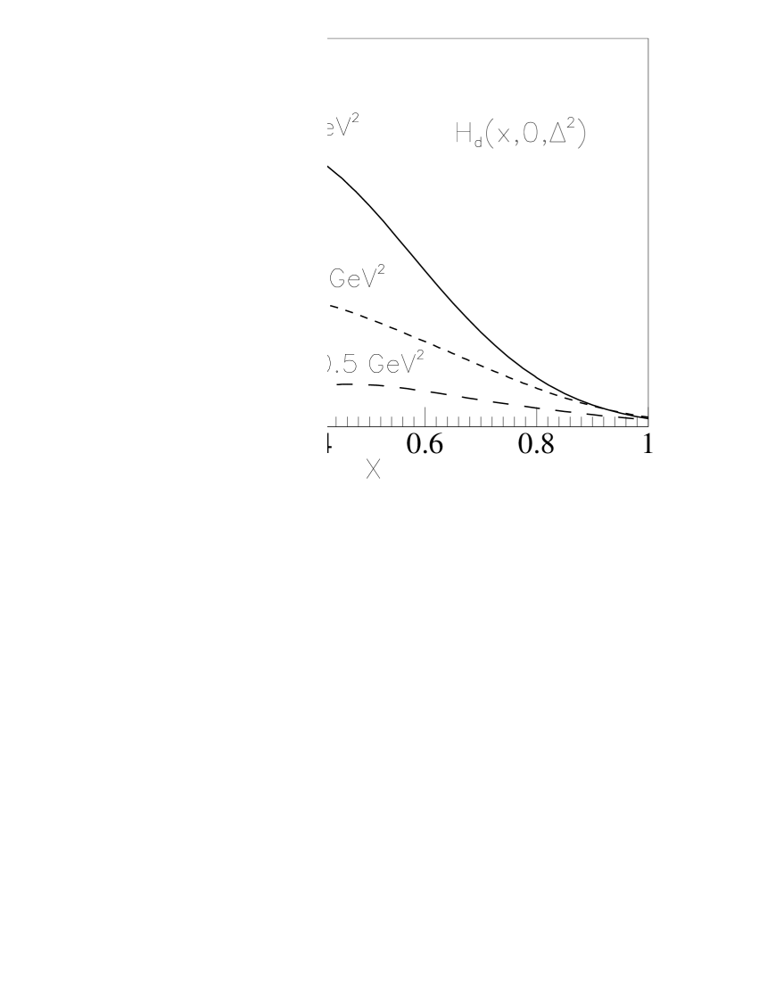
Figure 2:

Figure 3:

Figure 4:

Figure 5:

Figure 6:

Figure 7:

Figure 8:

References

- [1] X. Ji, J. Phys. G24 (1998) 1181.
- [2] A.V. Radyushkin, JLAB-THY-00-33, in M. Shifman, (ed.): At the frontier of particle physics, vol. 2, 1037-1099, hep-ph/0101225.
- [3] K. Goeke, M.V. Polyakov, M. Vanderhaeghen, Prog. Part. Nucl. Phys.47 (2001) 401.
- [4] M. Burkardt, Phys. Rev. D 62 (2000) 071503.
- [5] By M. Diehl, T. Feldmann, R. Jakob, P. Kroll Nucl. Phys. B596 (2001) 33; Phys. Lett. B460 (1999) 204.
- [6] X. Ji, Phys. Rev. Lett. 78 (1997) 610.
- [7] X. Ji, Phys. Rev. D 55 (1997) 7114.
- [8] R.L. Jaffe, A.V. Manohar, Nucl. Phys. B 337 (1990) 509.
- [9] “The Science Driving the 12 GeV Upgrade of CEBAF”, Jefferson Lab, February 2001.
- [10] J.M. Laget, Nucl. Phys. A666, (2000) 336.
- [11] X. Ji, W. Melnitchouk, and X. Song, Phys. Rev. D 56 (1997) 5511.
- [12] I.V. Anikin, D. Binosi, R. Medrano, S. Noguera, and V. Vento, Eur.Phys.J.A14 (2002) 95.
- [13] V.Yu. Petrov, P.V. Pobylitsa, M.V. Polyakov, I. Bornig, K. Goeke, C. Weiss, Phys. Rev. D57 (1998) 4325; M. Penttinen, M.V. Polyakov, K. Goeke, Phys. Rev. D62 (2000) 014024.
- [14] B.C. Tiburzi, G.A. Miller Phys. Rev. C64 (2001) 065204; hep-ph/0109174.
- [15] A. Freund, V. Guzey, Phys .Lett. B462 (1999) 178; L. Frankfurt, A. Freund, V. Guzey, M. Strikman Phys. Lett. B418 (1998) 345.
- [16] I.V. Musatov, A.V. Radyushkin, Phys. Rev. D61 (2000) 074027; A.V. Radyushkin Phys. Lett. B 449 (1999) 81.
- [17] A.V. Belitsky, B. Geyer, D. Muller, A. Schäfer Phys. Lett. B421 (1998) 312; A.V. Belitsky, D. Muller, L. Niedermeier, A. Schäfer Phys. Lett. B437 (1998) 160; Nucl.Phys. B546 (1999) 279; Phys. Lett. B474 (2000) 163.
- [18] A.V. Belitsky, A. Freund, D. Muller Nucl. Phys. B574 (2000) 347; Phys. Lett. B493 (2000) 341; A. Freund, M.F. McDermott Phys. Rev. D65 (2002) 056012; Phys. Rev. D65 (2002) 091901; Phys. Rev. D65 (2002) 074008; Eur. Phys. J. C23 (2002) 651.
- [19] A.V. Belitsky, A. Schäfer Nucl. Phys. B527 (1998) 235; N. Kivel, Maxim V. Polyakov, A. Schäfer, O.V. Teryaev Phys. Lett. B497 (2001) 73; A.V. Belitsky, A. Kirchner, D. Muller, A. Schäfer Phys. Lett. B510 (2001) 117.
- [20] M. Burkardt, hep-ph/0105324.
- [21] G. Parisi, R. Petronzio, Phys. Lett. B 62 (1976) 331.
- [22] R.L. Jaffe, G.G. Ross, Phys. Lett. B 93 (1980) 313.
- [23] M. Traini, V. Vento, A. Mair and A. Zambarda, Nucl. Phys. A 614 (1997) 472.
- [24] N. Isgur and G. Karl, Phys. Rev. D 18 (1978) 4187, D 19 (1979) 2653.
- [25] S. Scopetta and V. Vento, to be published.
- [26] V.N. Gribov and L. N. Lipatov, Sov. J. Nucl. Phys. 15, 78 (1972); L.N. Lipatov, Sov. J. Nucl. Phys. 20, 94 (1975); G. Altarelli and G. Parisi, Nucl. Phys. B126 (1977) 298; Yu.L. Dokshitser, Sov. Phys. JET, 46 (1977) 641.
- [27] A.V. Efremov and A.V. Radyushkin, Phys. Lett. B94 (1980) 245; S.J. Brodsky and G.P. Lepage, Phys. Rev. D22 (1980) 2157.
- [28] P. Mulders, Phys. Rept. 185 (1990) 83.
- [29] L. Conci and M. Traini, Few-Body Systems 8, 123-136 (1990).
- [30] M.M. Giannini, Rep. Prog. Phys. 54 (1991) 453.
- [31] G. Altarelli, N. Cabibbo, L. Maiani and R. Petronzio, Nucl. Phys. B 69 (1974) 531; G. Altarelli, S. Petrarca and F. Rapuano, Phys. Lett. B 373 (1996) 200.
- [32] F. Cardarelli, E. Pace, G. Salme, S. Simula Phys. Lett. B 357 (1995) 267.
- [33] S. Scopetta, V. Vento and M. Traini, Phys. Lett. B 421 (1998) 64; Phys. Lett. B 442 (1998) 28.
- [34] N. Isgur, G. Karl and R. Koniuk, Phys. Rev. Lett. 41 (1978) 1269; N. Isgur, G. Karl and J. Soffer, Phys. Rev. D 35 (1987) 1665.
- [35] M. Traini, L. Conci and U. Moschella, Nucl. Phys. A544 (1992) 781.
- [36] http://durpdg.dur.ac.uk/hepdata/dvcs.html
- [37] K.J. Golec-Biernat and A.D. Martin, Phys. Rev. D59 (1999) 014029.
- [38] M. Glück, E. Reya and A. Vogt, Eur. Phys. J. C5 (1998) 461 and reference therein.