Two Higgs Doublet Model, Standard Model–like scenario and resolving SM from 2HDM at Photon Colliders
Talk given at XVI Workshop on High Energy Physics and Quantum Field Theory, Moscow, September 2001

Abstract

1. Discussing 2HDM and Higgs potential, we find the parameters range giving naturally weak effects of CP violation and Flavor Changing Neutral Currents. Within this approach, the widely discussed decoupling limit with heavy $H^{\pm}$, $H$ and $A$ corresponds to an unnatural set of 2HDM parameters.

2. We define the SM–like scenario as that in which after LHC and $e^{+}e^{-}\,$ LC experiments no visible deviations from the minimal SM will be found. We find all the parameter ranges of 2HDM compatible with this scenario.

3. We show that the study of Higgs boson production at Photon Colliders (processes $\mbox{$\gamma\gamma\,$}\to h$ and $e\gamma\to eh\,$) can help to distinguish minimal SM from 2HDM with natural set of parameters.

1 Two Higgs Doublet Model

The different variants of Higgs type spontaneous electroweak symmetry breaking (EWSB) in the Standard Model are described by lagrangian

$$\begin{array}[]{l}{\cal L}={\cal L}^{SM}_{gf}+{\cal L}_{H}+{\cal L}_{Y}+V\,;\\[5.69054pt] {\cal L}^{SM}_{gf}\;\mbox{ -- SM interaction of gauge bosons and fermions}\,,\\[5.69054pt] {\cal L}_{H}=\sum\limits_{a}(D_{\mu}\phi_{a})^{\dagger}(D_{\mu}\phi_{a})\;\mbox{ -- scalar kinetic term}\,,\\[5.69054pt] {\cal L}_{Y}\;\mbox{ -- Yukawa interaction of fermions to scalars}\,,\\[5.69054pt] V\;\mbox{ -- Higgs potential}\,.\end{array}$$ (1)

In the Minimal Standard Model (SM) the single Higgs isodoublet ($a=1$) with hypercharge $Y=1$ is used. The simplest extension of SM is the Two Higgs Doublet Model (2HDM) with 2 complex scalar doublets ($a=1,2$). To keep for the quantity $\rho=M_{W}^{2}/(M_{Z}^{2}\cos^{2}\theta_{W})$ its SM value $\rho=1$ at tree level, both Higgs fields should be naturally weak isodoublets ($T=1/2$) with hypercharges $Y=\pm 1$. We use $Y=+1$ for both (the other choices, e.g. $Y_{1}=1,\;Y_{2}=-1$ – as in MSSM – keep our results up to redefinitions).

The Higgs sector, different from that in the minimal SM, generally gives CP violation ($\hbox to0.0pt{CP\hss}\,\diagup$  ) and Flavor Changing Neutral Currents (FCNC) at EWSB. In the 2HDM the $(\phi_{1},\,\phi_{2})$ mixing plays a crucial role in these violations. Let us summarize main points.

$\Box$ The Higgs potential generates CP violation only if $(\phi_{1},\,\phi_{2})$ mixing exists, and corresponding coefficients in potential are complex. We discuss this point in details below. $\Box$ $(\phi_{1},\,\phi_{2})$ mixing can also be originated from the Yukawa type interaction – if any fermions couple to both scalar fields, the one–loop polarization operator generates the $(\phi_{1},\,\phi_{2})$ mixing. Such Yukawa interaction naturally contains terms which are off–diagonal in family index giving potentially large FCNC effects.

It is well known that both $\hbox to0.0pt{CP\hss}\,\diagup$  and FCNC effects are weak. Therefore, the natural construction of 2HDM should start with the lagrangian having an additional symmetry forbidding the $\hbox to0.0pt{CP\hss}\,\diagup$  and FCNC effects, or ($\phi_{1},\phi_{2}$) mixing. This is $Z_{2}$ symmetry at

$$\phi_{1}\leftrightarrow-\phi_{1},\;\phi_{2}\leftrightarrow\phi_{2}\;\mbox{ and vice versa.}$$ (2)

This symmetry can be weakly broken to allow weak $\hbox to0.0pt{CP\hss}\,\diagup$  and FCNC effects. Therefore the terms in the lagrangian giving ($\phi_{1},\phi_{2}$) mixing have to be absent or small.

$\bullet$ Below we use ratios of actual coupling constants of each neutral Higgs scalar $\phi$ to particle $i$ to corresponding values for the Higgs boson in the SM,

$$\chi_{i}^{\phi}=\frac{{\displaystyle g_{i}^{\phi}}}{{\displaystyle g_{i}^{\rm SM}}}\Rightarrow\chi_{fS}^{\phi}+i\gamma^{5}\chi_{fA}^{\phi}\,.$$ (3a)

The latter form arises for fermions if Higgs–like boson has no definite CP parity, being a mixture of scalar and pseudoscalar.

If fermion mass $M_{f}$ is much lower than the mass of considered Higgs boson $M_{i}$, the partial width of corresponding decay is given practically by the quantity $|\chi_{f}^{2}|$,

$$\Gamma(h_{i}\to f\bar{f})=\Gamma^{SM}(h\to f\bar{f})\left[|\chi_{f}^{i}|^{2}+|\chi_{fA}^{i}|^{2}{\cal O}\left(\frac{{\displaystyle M_{f}^{2}}}{{\displaystyle M_{i}^{2}}}\right)\right]\,.$$ (3b)

1.1 Higgs potential

The most general Higgs potential in a renormalizable theory can be written as

$$\begin{array}[]{c}V=\frac{{\displaystyle\lambda_{1}}}{{\displaystyle 2}}(\phi_{1}^{\dagger}\phi_{1})^{2}+\frac{{\displaystyle\lambda_{2}}}{{\displaystyle 2}}(\phi_{2}^{\dagger}\phi_{2})^{2}+\lambda_{3}(\phi_{1}^{\dagger}\phi_{1})(\phi_{2}^{\dagger}\phi_{2})\\[5.69054pt] +\lambda_{4}(\phi_{1}^{\dagger}\phi_{2})(\phi_{2}^{\dagger}\phi_{1})+\frac{{\displaystyle 1}}{{\displaystyle 2}}\left[\lambda_{5}(\phi_{1}^{\dagger}\phi_{2})^{2}+h.c.\right]+\Delta V_{m}^{4}+{\cal M}(\phi_{i})+V_{0}\,;\\[5.69054pt] \Delta V_{m}^{4}=\left\{\left[\lambda_{6}(\phi_{1}^{\dagger}\phi_{1})+\lambda_{7}(\phi_{2}^{\dagger}\phi_{2})\right](\phi_{1}^{\dagger}\phi_{2})+h.c.\right\},\\[8.53581pt] {\cal M}(\phi_{i})=-\frac{{\displaystyle 1}}{{\displaystyle 2}}\left\{m_{11}^{2}(\phi_{1}^{\dagger}\phi_{1})+\left[m_{12}^{2}(\phi_{1}^{\dagger}\phi_{2})+h.c.\right]+m_{22}^{2}(\phi_{2}^{\dagger}\phi_{2})\right\},\quad V_{0}=const\,.\end{array}$$ (4)

Here $\lambda_{1-4}$, $m_{11}^{2}$ and $m_{22}^{2}$ are real, while parameters $\lambda_{5-7}$ and $m_{12}$ are generally complex. The constant $V_{0}$ is added to make vacuum energy equal to zero after EWSB.

To eliminate $(\phi_{1},\,\phi_{2})$ mixing, one should set $m_{12}=0$ and $\Delta V_{m}^{4}=0$. The term with $m_{12}$ describes soft violation of $Z_{2}$ symmetry. In our discussion limited to the tree level, additional contribution $\Delta V_{m}^{4}$ introduces no new phenomenology, it just complicates the equations. At the loop level the term $\Delta V_{m}^{4}$ causes certain difficulties in description of the model. By these reasons we omit this term in the forthcoming discussion (as many authors do ”for the sake of simplicity”).

$\Box$ The minimum of the potential defines vacuum expectation values $\langle\phi_{i}\rangle$ (v.e.v.’s) of the fields $\phi_{i}$ via equations

$$\frac{{\displaystyle\partial V}}{{\displaystyle\partial\phi_{i}}}\left(\phi_{1}=\langle\phi_{1}\rangle,\;\phi_{2}=\langle\phi_{2}\rangle\right)=0\;\mbox{ with }\langle\phi_{1}\rangle=\frac{{\displaystyle 1}}{{\displaystyle\sqrt{2}}}\left(\begin{array}[]{c}0\\ v_{1}\end{array}\right),\;\langle\phi_{2}\rangle=\frac{{\displaystyle 1}}{{\displaystyle\sqrt{2}}}\left(\begin{array}[]{c}0\\[14.22636pt] v_{2}e^{i\xi}\end{array}\right).$$ (5a)

The commonly used parameterization of v.e.v.’s is

$$v_{1}=v\cos\beta\,,\;\;v_{2}=v\sin\beta\,,\quad\beta\in(0,\,\frac{{\displaystyle\pi}}{{\displaystyle 2}})\,.$$ (5b)

The SM constraint $v=\left(G_{F}\sqrt{2}\right)^{-1/2}=246\mbox{ GeV}$ limits the parameters of potential.

$\blacksquare$ Let us express coefficients $m_{ij}^{2}$ in terms of $\lambda_{i}$ and v.e.v.’s, i.e. find them as solutions of eq-s (5a). It is useful to make it in two steps. We start with the case $m_{12}=0$ (with exact $Z_{2}$ symmetry), which gives $\hat{m}_{11}^{2}$ and $\hat{m}_{22}^{2}$ and equation $Im\left(\lambda_{5}e^{2i\xi}\right)=0$ for the phase $\xi$. Next, we find $m_{ij}^{2}-\hat{m}_{ij}^{2}$. This procedure contains ambiguity, parameterized by single additional parameter denoted as $\mu$:

$$\begin{array}[]{c}{\cal M}(\phi)=-\frac{{\displaystyle 1}}{{\displaystyle 2}}[\hat{m}^{2}_{11}(\phi_{1}^{\dagger}\phi_{1})+\hat{m}^{2}_{22}(\phi_{2}^{\dagger}\phi_{2})]+\frac{{\displaystyle\mu^{2}}}{{\displaystyle 2v^{2}}}\left(v_{2}e^{-i\xi}\phi_{1}^{\dagger}-v_{1}\phi_{2}^{\dagger}\right)\left(v_{2}e^{i\xi}\phi_{1}-v_{1}\phi_{2}\right)\\[11.38109pt] +iv_{1}v_{2}Im\left(\lambda_{5}e^{2i\xi}\right)[e^{-{i\xi}}\phi_{1}^{\dagger}\phi_{2}-h.c.]\,;\\[11.38109pt] \hat{m}^{2}_{11}=\lambda_{1}v_{1}^{2}+\lambda_{345}v_{2}^{2}\,,\;\;\hat{m}_{22}^{2}=\lambda_{2}v_{2}^{2}+\lambda_{345}v_{1}^{2}\,,\;\;(\lambda_{345}=\lambda_{3}+\lambda_{4}+Re\left(\lambda_{5}e^{2i\xi}\right))\,,\\[11.38109pt] \Rightarrow m_{11}^{2}=\hat{m}_{11}^{2}+\frac{{\displaystyle\mu^{2}v_{2}^{2}}}{{\displaystyle v^{2}}},\;m_{22}^{2}=\hat{m}_{22}^{2}+\frac{{\displaystyle\mu^{2}v_{1}^{2}}}{{\displaystyle v^{2}}},\;m_{12}^{2}=\left[-\frac{{\displaystyle\mu^{2}}}{{\displaystyle v^{2}}}+iIm(\lambda_{5}e^{2i\xi})\right]v_{1}v_{2}e^{-i\xi}.\end{array}$$ (6a)

These relations present the explicit form of eq-s (5a) for obtaining two v.e.v.’s $v_{1}$, $v_{2}$ (or $v$ and $\tan\beta$) and their relative phase $\xi$ via $m_{ij}$, $\lambda_{i}$ and $\mu$. The latter equation of (6a) gives $\xi$, it can be also written as

$$Im(m_{12}^{2}e^{i\xi})=Im(\lambda_{5}e^{2i\xi})v_{1}v_{2}\,.$$ (6b)

$\blacksquare$ The potential (4) is invariant under the rotations

$$\phi_{i}\to e^{i\rho_{i}}\phi_{i}\;\;(i=1,2),\;\;\lambda_{5}\to\lambda_{5}e^{2i(\rho_{2}-\rho_{1})}\,,\;\;m_{12}^{2}\to m_{12}^{2}e^{i(\rho_{2}-\rho_{1})}$$ (7a)

with $$\lambda_{1-4}\,,m_{11}\,,m_{22} \xi\to\xi+\rho_{1}-\rho_{2} \lambda_{5}e^{2i\xi} m_{12}^{2}e^{i\xi} \lambda_{1-4}$$ being constant. At this transformation the phase conventions (5) for v.e.v.’s are shifted as  and the quantities , , are invariant.

The Yukawa term is invariant under this transformation if in addition to (7a) fermion fields transform as

$$q_{iL}\to q_{iL}e^{i\theta_{i}}\,,\;\;U_{iR}\to U_{iR}e^{i(\theta_{i}-\rho_{iu})}\,,\;\;D_{iR}\to D_{iR}e^{i(\theta_{i}-\rho_{id})}\;\mbox{ with }iu,\,id=1\mbox{ or }2$$ (7b)

and off-diagonal in family index Yukawa couplings transform like eq. (7a).

Therefore, there is a family of potentials which give the same physics but differ in values of some parameters – phase family. The choice of definite term within the family is similar to gauge fixing for gauge fields. We denote this choice as phase gauge. In particular, one can consider the vacuum CP symmetric phase gauge, in which there is no ”spontaneous violation of CP symmetry of vacuum”, with $\xi=0$. In other words, the invariance mentioned above allows to eliminate phase $\xi$ from equations without changing the physically explicit CP violation (given by the mixing of scalar and pseudoscalar components of $\phi_{i}$ in the observable Higgs fields). To obtain this representation, we start with an arbitrary form of potential, and

$$\begin{array}[]{l}\bullet\mbox{ determine }v_{i}\mbox{ and }\xi\mbox{ via equations (\ref{solution}) ,}\\[5.69054pt] \bullet\mbox{ change }m_{12}^{2}\to m^{2}_{12,0}=m_{12}^{2}e^{i\xi}\,,\;\;\lambda_{5}\to\lambda_{5,0}=\lambda_{5}e^{2i\xi}\mbox{ in potential }.\end{array}$$ (8a)

In accordance with eq. (6b), new values $$m_{12}^{2} \lambda_{5}$$ and will be constrained by

$$Im(m_{12,0}^{2})=Im(\lambda_{5,0})v_{1}v_{2}\quad\mbox{ (at }\xi=0)\,.$$ (8b)

(In particular, for the $$Z_{2} m_{12}=0 \lambda_{5,0}$$ symmetric case we have and the quantity is real.)

We use below this phase gauge, in which the general Higgs potential (without $V^{4}_{m}$ term) adopts the form

$$\begin{array}[]{c}V=\frac{{\displaystyle\lambda_{1}}}{{\displaystyle 2}}(\phi_{1}^{\dagger}\phi_{1}-\frac{{\displaystyle v_{1}^{2}}}{{\displaystyle 2}})^{2}+\frac{{\displaystyle\lambda_{2}}}{{\displaystyle 2}}(\phi_{2}^{\dagger}\phi_{2}-\frac{{\displaystyle v_{2}^{2}}}{{\displaystyle 2}})^{2}+\lambda_{3}(\phi_{1}^{\dagger}\phi_{1}-\frac{{\displaystyle v_{1}^{2}}}{{\displaystyle 2}})(\phi_{2}^{\dagger}\phi_{2}-\frac{{\displaystyle v_{2}^{2}}}{{\displaystyle 2}})\\[11.38109pt] +\lambda_{4}(\phi_{1}^{\dagger}\phi_{2})(\phi_{2}^{\dagger}\phi_{1})+\left[\frac{{\displaystyle\lambda_{5,0}}}{{\displaystyle 2}}(\phi_{1}^{\dagger}\phi_{2})^{2}+h.c.\right]-\frac{{\displaystyle[\lambda_{4}+Re(\lambda_{5,0})][(\phi_{1}^{\dagger}\phi_{1})v_{2}^{2}+(\phi_{2}^{\dagger}\phi_{2})v_{1}^{2}]}}{{\displaystyle 2}}\\[11.38109pt] +\frac{{\displaystyle\mu^{2}}}{{\displaystyle 2v^{2}}}(v_{2}\phi^{\dagger}_{1}-v_{1}\phi^{\dagger}_{2})(v_{2}\phi_{1}-v_{1}\phi_{2})-iIm(\lambda_{5,0})v_{1}v_{2}\left(\phi^{\dagger}_{1}\phi_{2}-h.c.\right).\end{array}$$ (8c)

$\blacksquare$ The parameters of Higgs potential are limited by two types of conditions. First, the potential must be positive at large quasi–classical values of fields $|\phi_{i}|$ to have stable vacuum (positivity constraints). Constraints of the other type are related to the limits of the tree approximation applicability. It is correct when the radiative corrections (RC) to observable quantities are small. In this respect the perturbativity (or unitarity) limitations are considered. These constraints limit only our analysis. Therefore, it can happen that the RC for all observable quantities are small while RC to the parameters of heavy (non observed to the moment) Higgs bosons can be large.

1.2 Physical sector. CP violation.

The standard decomposition of fields $\phi_{i}$ in terms of physical fields is

$$\phi_{1}=\left(\begin{array}[]{c}\varphi_{1}^{+}\\[5.69054pt] \frac{{\displaystyle 1}}{{\displaystyle\sqrt{2}}}(v_{1}+\eta_{1}+i\chi_{1})\end{array}\right),\qquad\phi_{2}=\left(\begin{array}[]{c}\varphi_{2}^{+}\\[5.69054pt] \frac{{\displaystyle 1}}{{\displaystyle\sqrt{2}}}(v_{2}e^{i\xi}+\eta_{2}+i\chi_{2})\end{array}\right).$$ (9)

The combinations $G^{0}=\chi_{1}\cos\beta+\chi_{2}\sin\beta$ and $G^{\pm}=\phi_{1}^{\pm}\cos\beta+\phi_{2}^{\pm}\sin\beta$ describe Goldstone bosons. In the CP conserving case (at $Im(m_{12,0}^{2})=0$) the physical Higgs sector of 2HDM contains two charged Higgs bosons $H^{\pm}$, one CP-odd (pseudoscalar) $A$ and two CP-even scalars $h$ and $H$ with $M_{H}>M_{h}$

$$\begin{array}[]{c}A=-\chi_{1}\,\sin\beta+\chi_{2}\,\cos\beta\,,\quad H^{\pm}=-\varphi_{1}^{\pm}\,\sin\beta+\varphi_{2}^{\pm}\,\cos\beta\,,\\[11.38109pt] H=\eta_{1}\,\cos\alpha+\eta_{2}\,\sin\alpha\,,\quad h=-\eta_{1}\,\sin\alpha+\eta_{2}\,\cos\alpha\,;\quad\alpha\in(-\pi/2,\,\pi/2)\,.\end{array}$$ (10)

In the general $\hbox to0.0pt{CP\hss}\,\diagup$  case we have the same charged Higgs bosons with mass $M_{H^{\pm}}^{2}=\mu^{2}-(\lambda_{4}+Re(\lambda_{5,0}))v^{2}/2$ and three neutral scalar states $h_{1}$, $h_{2}$, $h_{3}$ having no definite CP parity (with convention $M_{h_{3}},\,M_{h_{2}}\geq M_{h_{1}}$). These $M_{h_{i}}^{2}$ are obtained from $\eta_{1}$, $\eta_{2}$ and $A$ by diagonalization of the mass matrix $M$

$$\begin{array}[]{c}M=\left(\begin{array}[]{ccc}M_{11}&M_{12}&\delta\sin\beta\\[11.38109pt] M_{12}&M_{22}&\delta\cos\beta\\[11.38109pt] \delta\sin\beta&\delta\cos\beta&\mu^{2}-Re(\lambda_{5,0})v^{2}\end{array}\right)\\[11.38109pt] \\ M_{11}=\mu^{2}\sin^{2}\beta+\lambda_{1}v^{2}\cos^{2}\beta,\;\;M_{22}=\mu^{2}\cos^{2}\beta+\lambda_{2}v^{2}\sin^{2}\beta,\\[11.38109pt] M_{12}=(\lambda_{345}v^{2}-\mu^{2})\frac{{\displaystyle sin2\beta}}{{\displaystyle 2}},\;\;\lambda_{345}=\lambda_{3}+\lambda_{4}+Re\lambda_{5,0}\,;\quad\delta=\frac{{\displaystyle Im(\lambda_{5,0})v^{2}}}{{\displaystyle 2}}\,.\end{array}$$ (11)

These states are determined with the aid of unitary transition matrix $R$, written through Euler angles $\alpha_{i}$ ($c_{i}=\cos\alpha_{i},\;\;s_{i}=\sin\alpha_{i}$):

$$\begin{array}[]{c}\left(\begin{array}[]{c}h_{1}\\ h_{2}\\ h_{3}\end{array}\right)=R\left(\begin{array}[]{c}\eta_{1}\\ \eta_{2}\\ A\end{array}\right),\;\;R=\left(\begin{array}[]{ccc}-s_{1}&c_{1}c_{2}&-c_{1}s_{2}\\ -c_{1}s_{3}&\;s_{2}c_{3}-s_{1}c_{2}s_{3}&s_{1}s_{2}s_{3}+c_{2}c_{3}\\ c_{1}c_{3}&s_{1}c_{2}c_{3}+s_{2}s_{3}&c_{2}s_{3}-s_{1}s_{2}c_{3}\end{array}\right).\\[22.76219pt] \left(\mbox{At }\;\alpha_{2},\;\alpha_{3}\to 0\Rightarrow\alpha_{1}\to\alpha,\;\;h_{1}\to h,\;\;h_{2}\to H,\;\;h_{3}\to A\right)\,.\end{array}$$ (12)

$\bullet$ In the CP conserving case the masses of neutral Higgs particles and mixing angle $\alpha$ are obtained by diagonalization of mass matrix $M$ (11) with $\delta=0$:

$$\begin{array}[]{c}\begin{array}[]{c}M_{A}^{2}=\mu^{2}-Re(\lambda_{5,0})v^{2},\quad M_{H^{\pm}}^{2}=\mu^{2}-\frac{{\displaystyle 1}}{{\displaystyle 2}}(Re(\lambda_{5,0})+\lambda_{4})v^{2},\\[11.38109pt] M_{h,H}^{2}=\frac{{\displaystyle 1}}{{\displaystyle 2}}\left(M_{11}+M_{22}\mp R\right),\quad R=\sqrt{(M_{11}-M_{22})^{2}+4M_{12}^{2}},\\[11.38109pt] M_{H}^{2}+M_{h}^{2}=\mu^{2}+\frac{{\displaystyle 1}}{{\displaystyle 2}}[(\lambda_{1}+\lambda_{2})+(\lambda_{1}-\lambda_{2})\cos 2\beta]v^{2}\,.\end{array}\end{array}$$ (13a)

These equations can be accompanied by useful relations:

$$\sin 2\alpha=\frac{{\displaystyle 2M_{12}}}{{\displaystyle R}},\quad\cos 2\alpha=\frac{{\displaystyle M_{11}-M_{22}}}{{\displaystyle R}}\,,\;\;M_{H}^{2}-M_{h}^{2}=\frac{{\displaystyle\sin 2\beta}}{{\displaystyle\sin 2\alpha}}\left(-\mu^{2}+\lambda_{345}v^{2}\right)\,.$$ (13b)

$\bullet$ In the case of weak ($\phi_{1},\,\phi_{2}$) mixing, i.e. small value of $m_{12}$ and respectively $\delta$, one can obtain the neutral Higgs boson masses in the form of corrections $\sim\delta^{2}$ to the expressions (13a),

$$\begin{array}[]{c}M_{1}^{2}=M_{h}^{2}-\frac{{\displaystyle\delta^{2}}}{{\displaystyle 2(M_{A}^{2}-M_{h}^{2})}}(1+t)\,,\quad M_{2}^{2}=M_{H}^{2}-\frac{{\displaystyle\delta^{2}}}{{\displaystyle 2(M_{A}^{2}-M_{H}^{2})}}(1-t)\,,\\[8.53581pt] M_{3}^{2}=M_{A}^{2}+M_{H}^{2}+M_{h}^{2}-M_{1}^{2}-M_{2}^{2}\,,\quad t=\frac{{\displaystyle(M_{11}-M_{22})\cos 2\beta-M_{12}\sin 2\beta}}{{\displaystyle M_{H}^{2}-M_{h}^{2}}}\,.\end{array}$$ (13c)

Similarly, one can easily obtain small mixing angles $\alpha_{2}$ and $\alpha_{3}$ just as $\alpha_{1}-\alpha$ in this case.

$\blacksquare$ Some couplings. The couplings of Higgs particles to vector bosons are written via elements of transition matrix $R$ (12):

$$\chi_{V}^{h_{i}}=s_{\beta}R_{i2}+c_{\beta}R_{i1}\,.$$ (14)

As well as other trilinear couplings, the coupling of charged Higgs boson to the neutral Higgs boson is written via $\lambda_{i}$ and $v_{i}$, without $\mu$. Hereafter it is useful to present this coupling in terms of observable masses and $\mu$, in units of the coupling of the Higgs particle $\phi=h$ (or $H$) to an arbitrary scalar particle with mass equal to $M_{H^{\pm}}$ added to the SM. For the CP conserving case that is

$$\chi_{H^{\pm}}^{\phi}\equiv-\frac{{\displaystyle vg_{\phi H^{+}H^{-}}}}{{\displaystyle 2M_{H^{\pm}}^{2}}}=\left(1-\frac{{\displaystyle M_{\phi}^{2}}}{{\displaystyle 2M_{H^{\pm}}^{2}}}\right)\sin(\beta-\alpha)+\frac{{\displaystyle(M_{\phi}^{2}-\mu^{2})\cos(\beta+\alpha)}}{{\displaystyle M_{H^{\pm}}^{2}\sin 2\beta}}\,.$$ (15)

1.3 Different scenarios in 2HDM, natural range of parameters.

The widely discussed scenario for Higgs sector is that there exists one light Higgs boson $h_{1}$ which is near discovery reach of present accelerators, and other possible Higgs bosons are very heavy. In accordance with eqs. (13), it can takes place if

$\bf 1.$ $|m_{12}|$ is small ($\mu\lesssim v$), i.e. $Z_{2}$ symmetry is precise or weakly broken. Some Higgs bosons can be heavy due to large values of couplings $\lambda_{i}$, their values are limited from above by perturbativity limitation for $\lambda_{i}$ at the level $4\pi v\approx 3$ TeV. In particular, if additionally CP is conserved and masses of $H$, $A$, $H^{\pm}$ are about 800 GeV, for the parameters of perturbation theory we have $|\lambda_{5}|/(4\pi)^{2}$, $\lambda_{4}|/(4\pi)^{2}$, $|\lambda_{345}|/(4\pi)^{2}\approx 0.07$. These values lie within the perturbativity domain.

$\bf 2.$ $\mu$ is large ($\mu^{2}\gg\lambda_{i}v^{2}\,,M_{h}^{2}$), i.e. $Z_{2}$ symmetry is strongly broken. In this case high values of masses are given by high value of parameter $\mu$ even at relatively small Higgs boson self–couplings $\lambda_{i}$. Besides, in this case due to eqs. (13),

• Heavy Higgs bosons $H$, $A$ (or $h_{2}$, $h_{3}$) and $H^{\pm}$ are almost degenerate in their masses.

• Comparing the last equations (13a) and (13b), in the CP conserving case we have $\sin 2\alpha\approx-\sin 2\beta$. Since $\beta\in(0,\pi/2)$ and $\alpha\in(-\pi/2,\pi/2)$, it gives two cases:

  • $2\alpha\approx 2\beta-\pi\Rightarrow\sin(\beta-\alpha)\approx 1$. It makes coupling constants of the lightest Higgs $h$ to the gauge bosons and quarks (in Model II) be close to their SM values. This very case is treated usually as decoupling limit [7].

  • $\alpha\approx-\beta$. This solution gives couplings of Higgs boson to gauge fields and quarks which are generally far from their SM values.

$\bullet$ The eq. (11) shows explicitly that the $\hbox to0.0pt{CP\hss}\,\diagup$  can take place only if $Im(m_{12,0}^{2})\neq 0$, i.e. in the case when $\phi_{1}$ and $\phi_{2}$ are mixed. The observed weak $\hbox to0.0pt{CP\hss}\,\diagup$  means relatively small value of $Im(m_{12}^{2})$ in the specific ”vacuum CP conserving phase gauge (7)”. This condition is natural, i.e. it can be formulated independently on phase gauge if $|m_{12}|$ is also small, and it looks as unnatural phase gauge dependent condition if $|m_{12}|$ is not small (for the decoupling limit). The similar discussion of FCNC is given below.

Therefore, a weak $\hbox to0.0pt{CP\hss}\,\diagup$  and FCNC effects naturally correspond to the case $|m_{12}|\ll v$, i.e. the case of weak $Z_{2}$ symmetry breaking (first opportunity above), and they are unnatural  for the the decoupling limit.

The discussed opportunities are summarized in the Table 1.

	basic relations in		small $\hbox to0.0pt{CP\hss}\,\diagup$	specific
	${\cal L}$ (4)	${\cal L}$ (8c)	and FCNC	features
weakly	$|m_{12}^{2}|\lesssim v^{2}$	$\mu^{2}\lesssim v^{2}$,	natural	$M_{2,3},\,M_{H^{\pm}}<3$ TeV,
broken		$Im\left(m_{12,0}^{2}\right)\lesssim v^{2}$		$\;\;\chi_{H^{\pm}}\sim 1$
$Z_{2}$ symmetry
decoupling	$Re\left(m_{12}^{2}e^{i\xi}\right)\gg v^{2}$,	$\mu^{2}\gg v^{2}$,	unnatural	$M_{2,3}\approx M_{H^{\pm}}$,
limit	$Im\left(m_{12}^{2}e^{i\xi}\right)$	$Im\left(m_{12,0}^{2}\right)$		$\;\;\chi_{H^{\pm}}\ll 1$

Table 1: Scenarios of 2HDM considered as natural in this paper and in some other papers.

1.4 Coupling to fermions (Yukawa interaction)

To avoid ($\phi_{1},\,\phi_{2}$) mixing at the one loop level, each type of quarks or leptons should acquire mass via only one Higgs field

$$\begin{array}[]{c}{\cal L}_{Y}^{0}=\sum\limits_{i}g_{i}^{d}\bar{q}_{iL}\phi_{id}D_{iR}+\sum\limits_{i}g_{i}^{u}\bar{q}_{iL}\phi_{iu}U_{iR}+h.c.+\mbox{lepton items}\\[5.69054pt] \mbox{with some of }iu,id,i\ell=1\;\mbox{ and other }=2\,.\end{array}$$ (16)

Two variants of this type are widely discussed in the literature (cf. [4]), these are Model I with $id=iu=i\ell=1$ and Model II considered below.

If Higgs potential contains ($\phi_{1},\,\phi_{2}$) mixed terms, there are no grounds to have Yukawa interaction in the form (16). Each fermion can be coupled to both Higgs bosons, and Yukawa interaction can be even off-diagonal in family index, giving FCNC. Assuming violation of $Z_{2}$ symmetry to be weak, we can consider these off–diagonal terms to be small. For Model I similar approach was developed in [8]. We neglect these small $Z_{2}$ symmetry violating Yukawa interactions in our discussion of Higgs sector itself.

$\blacksquare$ Model II (2HDM (II)).

We consider in detail the Model II in which the couplings to fermions are similar to those in MSSM. In this model, the fundamental scalar field $\phi_{1}$ couples to $u$-type quarks, while $\phi_{2}$ – to $d$-type quarks and charged leptons (we assume neutrinos to be massless),

$${\cal L}_{Y}^{0}=\sum\limits_{i}g_{i}^{d}\bar{q}_{iL}\phi_{2}D_{iR}+\sum\limits_{i}g_{i}^{u}\bar{q}_{iL}\phi_{1}U_{iR}+\sum\limits_{i}g_{i}^{\ell}\bar{\ell}_{iL}\phi_{2}E_{iR}+h.c.\,$$ (17)

Here the ratios, relative to the SM values, of the direct coupling constants of the Higgs boson $h_{i}$ to the gauge bosons $V=W$ or $Z$, to up and down quarks (3) (basic couplings) are given by elements of transition matrix $R$ (12) as (14)

$$\chi^{i}_{u}=\frac{{\displaystyle R_{i2}-i\gamma^{5}\cos\beta R_{i3}}}{{\displaystyle\sin\beta}}\,,\quad\chi^{i}_{d}=\frac{{\displaystyle R_{i1}-i\gamma^{5}\sin\beta R_{i3}}}{{\displaystyle\cos\beta}}\,.$$ (18)

$\Box$ It is also useful to write coupling constants of neutral scalars $\phi=h$ or $H$ to charged Higgs boson (15) via couplings of these scalars to fermions. In the CP conserving case

$$\chi_{H^{\pm}}^{\phi}\equiv-\frac{{\displaystyle vg_{\phi H^{+}H^{-}}}}{{\displaystyle 2M_{H^{\pm}}^{2}}}=\left(1-\frac{{\displaystyle M_{\phi}^{2}}}{{\displaystyle 2M_{H^{\pm}}^{2}}}\right)\chi_{V}^{\phi}+\frac{{\displaystyle M_{\phi}^{2}-\mu^{2}}}{{\displaystyle 2M_{H^{\pm}}^{2}}}(\chi_{u}^{\phi}+\chi_{d}^{\phi})\,,\quad(\phi=h\mbox{ or }H)\,.$$ (19)

The difference between two scenarios for mass generation of sect. 1.3   influences strongly this coupling. It is clearly seen that for the lightest Higgs boson in the first scenario (with natural $\hbox to0.0pt{CP\hss}\,\diagup$  and FCNC) $\chi_{H^{\pm}}\approx\chi_{V}\sim 1$ while for the decoupling limit $\chi_{H^{\pm}}\ll 1$. The measurement of the Higgs boson production in $\gamma\gamma\,$ collisions can distinguish these two mechanisms in the experiments at Photon Colliders [2]. (Note that direct measurements of separate Higgs self–couplings may be difficult).

$\blacksquare$ Pattern relation and sum rules.

$\bullet$ The unitarity of matrix $R$ allows to obtain a simple relation on couplings of one Higgs particle to gauge bosons and quarks, which is very useful at the phenomenological analysis, – pattern relation [2, 3], having the same form for each Higgs boson $h_{i}$:

$$(\chi_{u}+\chi_{d})\chi_{V}=1+\chi_{u}\chi_{d}.$$ (20)

It is also useful to express $\tan\beta$ via these couplings:

$$\tan^{2}\beta={\frac{{\displaystyle(\chi_{V}-\chi_{d})^{\dagger}}}{{\displaystyle\chi_{u}-\chi_{V}}}}\,.$$ (21)

$\bullet$ It can be obtained that unitarity of the matrix $R$ brings also the sum rules for each neutral Higgs boson [5]:

$$|\chi_{u}|^{2}\sin^{2}\beta+|\chi_{d}|^{2}\cos^{2}\beta=1\,.$$ (22)

These sum rules guarantee that the production cross sections for each neutral Higgs boson of 2HDM cannot be lower than that for the SM Higgs boson with the same mass at least in one commonly discussed process [5].

2 Standard Model-like scenario

We now consider the following scenario, referred below to as the SM-like scenario. It is defined by the following criteria:

1. One Higgs boson will be discovered (with mass above today’s limit for the SM Higgs boson, 115 GeV). It can either be the Higgs boson of the SM or one of several neutral scalars of another model, such as 2HDM.

2. No other Higgs boson will be discovered. That means, that other possible scalars are either
$\Box$ weakly coupled to the $Z$ and $W$ bosons, gluons and quarks, or
$\Box$ heavy enough to escape (direct or indirect) observation, e.g. $M_{H^{\pm}}>{\cal O}(800\mbox{ GeV})$.

3. Any other new particles that may exist are heavier than the discovery limits of LHC and the $e^{+}e^{-}$ Linear Collider.

4. The measured decay widths of the observed Higgs boson (or the squared coupling constants) to other particles, $\Gamma_{i}^{\rm exp}$, will be in agreement with their SM values $\Gamma_{i}^{\rm SM}$ within the to-date precision $\delta_{i}$, i.e.

$$\left|\frac{\Gamma_{i}^{\rm exp}}{\Gamma_{i}^{\rm SM}}-1\right|\lesssim\delta_{i}\ll 1.$$ (23a)

For the coupling constants themselves in terms of (3a), the eq. (23a) means that

$$\chi_{i}=\pm(1-\epsilon_{i})\;\mbox{ with }|\epsilon_{i}|\leq\delta_{i}\,.$$ (23b)

2.1 SM-like realizations in the 2HDM (II)

Even in the simplest extension of SM, the 2HDM, the SM-like scenario can be realized in many regions in the parameter space. We consider in detail the CP conserving case. There are two classes of solutions denoted $A_{\phi\pm}$ and $B_{\phi\pm q}$. Here the first subscript labels the observed Higgs boson and second subscript labels the sign of $\chi_{V}^{\phi}$. For the solutions $A_{H\pm}$, $B_{H\pm q}$ the analysis includes also the veto for the discovery of the lightest Higgs boson in the associated production with $t$ or $b$ quarks. More detailed analysis is available, for example, in [3].

For solutions $A_{\phi\pm}$ basic couplings of observed Higgs boson are approximately identical, $\chi_{V}^{\phi}\approx\chi_{u}^{\phi}\approx\chi_{d}^{\phi}\approx\pm 1$. For example, the solution $A_{H-}$ is that with the observed Higgs boson being the heaviest one, $H$, and with $\chi_{V}^{H}\approx-1$. (The decoupling limit can be realized for solution $A_{h+}$.) The exact solutions of these types $|\chi_{i}|=1$ can also be realized.

For solutions $B_{\phi\pm q}$ some of basic $\chi_{i}\approx 1$ but other $\chi_{j}\approx-1$. The third subscript $q=d,u$ denotes the type of quark whose coupling with the observed Higgs boson is of opposite sign as compared to the gauge boson coupling, $\chi_{V}$. (The solutions with $-\chi_{V}\approx\chi_{d}\approx\chi_{u}\approx\pm 1$ cannot be realized.) The exact solutions of these types $|\chi_{i}|=1$ cannot be realized, the conditions $\epsilon_{V}\neq 0$ and $\tan\beta\gg 1$ or $\ll 1$ are necessary in these cases. Note that these solutions cannot be realized at the decoupling limit, for all of them there should be $\mu\lesssim v$.

The allowed realizations of the SM-like scenario in the CP conserving case in 2HDM (II) are listed in the Table 2. The numbers in the table correspond to (1) the observed Higgs boson having the mass 115-180 GeV, considering higher masses of this boson for completeness; (2) usage of the anticipated inaccuracies for the Higgs boson couplings to quarks and gauge bosons at the $e^{+}e^{-}$ Linear Collider [9].

		observed
type	notation	Higgs	$\chi_{V}$	$\tan\beta$		constraint
		boson
	$A_{h+}$	h	$\approx+1$		$\lessgtr 1$
$A_{\phi\pm}$	$A_{H+}$	H	$\approx+1$		$\lessgtr 1$
$\chi_{V}\approx\chi_{u}\approx\chi_{d}$	$A_{h-}$	h	$\approx-1$	$\sqrt{\left|\frac{{\displaystyle\epsilon_{d}}}{{\displaystyle\epsilon_{u}}}\right|}$	$\ll 1$	$\epsilon_{V}=-\frac{{\displaystyle\epsilon_{u}\epsilon_{d}}}{{\displaystyle 2}}$
	$A_{H-}$	H	$\approx-1$		$\gg 1$
$B_{\phi\pm d}:$	$B_{h+d}$	h	$\approx+1$	$\sqrt{\frac{{\displaystyle 2}}{{\displaystyle\epsilon_{V}}}}\gtrsim 10$		$\epsilon_{u}=-\frac{{\displaystyle\epsilon_{V}\epsilon_{d}}}{{\displaystyle 2}}$
$\chi_{V}\approx\chi_{u}\approx-\chi_{d}$	$B_{H\pm d}$	H	$\approx\pm 1$
$B_{\phi\pm u}:$	$B_{h\pm u}$	h	$\approx\pm 1$	$\sqrt{\frac{{\displaystyle\epsilon_{V}}}{{\displaystyle 2}}}\lesssim 0.1$		$\epsilon_{d}=-\frac{{\displaystyle\epsilon_{V}\epsilon_{u}}}{{\displaystyle 2}}$
$\chi_{V}\approx\chi_{d}\approx-\chi_{u}$	$B_{H+u}$	H	$\approx+1$
$\chi_{i}=\frac{{\displaystyle g_{i}}}{{\displaystyle g_{i}^{SM}}}=\pm(1-\epsilon_{i})$ with
$i=V(\equiv Z,\,W)$ or $i=u(\equiv t,\,c)$ or $i=d,\ell(\equiv b,\,\tau);\quad\epsilon_{V}>0$, $\epsilon_{u}\epsilon_{d}<0$ .

Table 2: Allowed realizations of SM-like scenario in the 2HDM (II)

3 Resolving SM-like scenarios via Higgs boson production at a Photon Collider

Study of Higgs-boson couplings with photons ($h\gamma\gamma$ and $hZ\gamma$) is a very promising tool for resolving the models of New Physics by the following reasons.

$\bullet$ These couplings are absent in the SM at tree level, appearing only at the loop level. Therefore, the background for signals of New Physics here will be relatively lower than in other processes allowed at tree level of the SM.

$\bullet$ All fundamental charged particles contribute to these effective couplings. The whole structure of the theory influences the corresponding Higgs-boson decays. Note that for the contributions of heavy particles with masses given by the Higgs mechanism (like in minimal SM), there is no decoupling in these vertices.

$\bullet$ The anticipated accuracy in the measurements of $\Gamma(H\to\mbox{$\gamma\gamma\,$})$ in the $\mbox{$\gamma\gamma\,$}\to h$ process at Photon Collider is $\sim 2$% with the luminosity integral 30 fb^-1 and $M_{h}\leq 150$ GeV [10], [9]. It can be reduced to 1 % level with the anticipated luminosity integral about 500 fb^-1. Another possible opportunity to study these effects is provided by the $hZ\gamma$ interactions with the best potential for studying in the process $e\gamma\to eh$. Certainly, possible accuracy here is lower than in the $\gamma\gamma\,$ channel.

3.1 2HDM vs. SM

Of course, the best place for the comparison of models is given by the Higgs boson production in $\gamma\gamma\,$ collisions. We calculated these $h\mbox{$\gamma\gamma\,$}$ vertices in [2, 3]. Besides, we obtained there the $hZ\gamma$ decay width deviations from SM which are similar to those found for $\gamma\gamma\,$ channel but lower in value. The impression was: the $hZ\gamma$ vertex is unsuitable for resolving the models. However, this vertex participates in description of the process $e\gamma\to eh\,$  very far from the mass shell. Thus, we consider here this process to check the prediction above.

The process $e\gamma\to eh\,$ is described with diagrams: (i) $\mbox{$e\gamma\,$}\to(e\gamma^{*})\gamma\otimes\gamma^{*}\gamma\to h$ (photon exchange); (ii) $\mbox{$e\gamma\,$}\to(eZ^{*})\gamma\otimes Z^{*}\gamma\to h$ ($Z$ exchange); (iii) box diagrams; the latter give small contributions. This subdivision is approximately gauge invariant. Therefore, separate terms have physical sense [11].

In the total cross section of $e\gamma\to eh\,$ process the diagram with photon exchange is dominant. At $p_{\bot}(e)>30$ GeV the photon and $Z$ contributions become comparable, giving very different cross sections for the left-hand and right-hand polarized electrons, $\sigma_{L}>3\sigma_{L}$ [11]. Therefore, we present only results for $\sigma_{L}$ integrated over the region $p_{\bot}(e)>30$ GeV for $\sqrt{s_{e\gamma}}=1.5$ TeV (note that energy dependence becomes weak at large enough energy).

We calculated the relative widths $|\chi_{\gamma\gamma}|^{2}$ and the $\sigma_{L}(\mbox{$e\gamma\,$}\to eh)$ for all allowed realizations of SM-like scenario in 2HDM assuming natural form of Higgs potential, with $\mu\lesssim v$. For definiteness, we perform all calculations for $\mu=0$, $M_{H^{\pm}}=800$ GeV. In accordance with eq. (19), at $M_{i}<250$ GeV the contribution of the charged Higgs boson loop varies by less than 5% when $M_{H^{\pm}}$ varies from 800 GeV to infinity.

In the figures with the results, (i) solid curves correspond to the exact case, where all basic $|\chi_{i}|=1$; (ii) the shaded bands are derived from anticipated (in [9]) 1 $\sigma$ bounds for the measured basic coupling constants, $g_{V}$, $g_{u}$ and $g_{d}$, with additional constraints given by the pattern relation for each solution (Table 2).

Solutions A. A new feature of the considered widths and cross sections in the 2HDM compared to the SM case is the contribution from the charged Higgs boson loops. The results are shown in Figure 1.

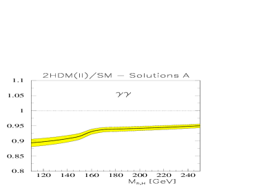
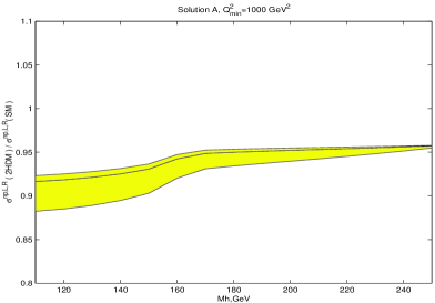
Figure 1: Solutions A and $B_{\phi\pm d}$. The ratio of quantities in 2HDM to their SM values. The two-photon Higgs width – left panel; the cross section $\sigma_{L}(e\gamma\to eh)$ – right panel.

Solutions B. For solutions $B$ we have, by definition, $\chi_{u}+\chi_{d}={\cal O}(\epsilon)$. So with high accuracy $\chi_{H^{\pm}}\approx\chi_{V}$. The results are shown in Figure 2. At the left panel (for $\gamma\gamma\,$) the lower curves correspond to the solutions $B_{\phi\pm d}$ and the upper ones to the solution $B_{h+u}$. At the right panel (for $e\gamma\to eh\,$) we show the SM and 2HDM cross sections themselves.

$\bullet$ For the solutions $B_{\phi\pm d}$ the main source of deviation from SM predictions is charged Higgs contribution. The effect of the opposite relative sign of the $b$-quark coupling ($\chi_{d}\simeq-\chi_{V}$) as compared to that in the SM case is negligible, since this contribution is very small itself. Therefore, the curves for this case coincide with those for solutions A (Fig. 1) with only note that the exact solution cannot be realized in this case. The result for the $\mbox{$\gamma\gamma\,$}\to h$ transition is also shown in the lower curve of left panel in Fig. 2

$\bullet$ For the solution $B_{h+u}$ the photon widths increase dramatically as compared to the SM case. Here, solid curve corresponds to the case $\chi_{V}=\chi_{d}=-\chi_{u}=1$, and $t$–quark contribution is smaller than that from $W$–boson, but it is about 20% from the $W$-boson one, and change of its sign becomes essential (Fig. 2).

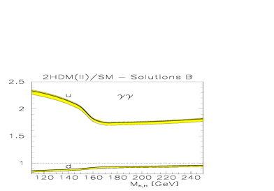
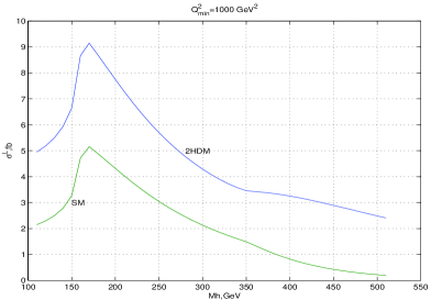
Figure 2: Solutions B — the ratio of two-photon widths in 2HDM to their SM values – left panel. The solution $B_{h+u}$ — the cross section $\sigma_{L}(e\gamma\to eh)$ in 2HDM and SM – right panel.

4 Conclusion and final notes

Let us summarize main conclusions.

1. The general 2HDM, in which strong CP violation and large FCNC effects are naturally suppressed, corresponds to small ($\phi_{1},\,\phi_{2}$) mixing, i.e. differs substantially from the option considered usually in context of decoupling limit.

2. Possible SM–like scenario includes the picture considered in the description of decoupling limit and allows many other realizations.

3. The comparison of the presented results with the anticipated experimental uncertainty shows that the deviation of the two-photon width from its SM value is generally large enough to allow a reliable distinction of the natural 2HDM (II) from the SM at the Photon Collider. The $e\gamma\to eh\,$ process can supplement this potential substantially, at least at $M_{h}<160$ GeV.

4. Solutions $B_{\phi\pm u}$ are separated well enough even for more rough measurements and independent on possible strong CP violation and FCNC.

5. We don’t see a way in such measurements to distinguish the cases when the observed Higgs boson is the lightest one $h$ ($h_{1}$) or the heaviest one, $H$ ($h_{2}$ or $h_{3}$).

Most part of results reported here was obtained in collaboration with M. Krawczyk and P. Osland. We are grateful to them for this fruitful collaboration. We are grateful to A. Djouadi, J. Gunion, H. Haber and M. Spira for discussions of decoupling in the 2HDM and the MSSM, and to P. Chankowski, W. Hollik, I. Ivanov, A. Pak for valuable discussions of the parameters of the 2HDM. This research has been supported by RFBR grants 99-02-17211 and 00-15-96691, INTAS grant 00-00679.

References

• [1] I.F. Ginzburg, M. Krawczyk, P. Osland, in preparation.
• [2] I.F. Ginzburg, M. Krawczyk, P. Osland, Proc. 4th Int. Workshop on Linear Colliders, April 28-May 5, 1999; Sitges (Spain) p. 524, (hep-ph/9909455); I.F. Ginzburg, Nucl. Phys. B (Proc. Suppl.) 82, 367 (2000); hep-ph/9907549.
• [3] I.F. Ginzburg, M. Krawczyk, P. Osland, hep-ph/0101208; Nucl. Instrum. Methods A 472 (2001) 149, hep-ph/0101229; hep-ph/0101331
• [4] J.F. Gunion, H.E. Haber, G. Kane, S. Dawson, The Higgs Hunter’s Guide (Addison-Wesley, Reading, 1990).
• [5] B. Grza̧dkowski, J.F. Gunion, J. Kalinowski, Phys. Rev. D 60, 075011 (1999); Phys. Lett. B 480, 287 (2000).
• [6] J. Liu, L. Wolfenstein, Nucl. Phys.  B289 (1987) 1.
• [7] H.E. Haber, hep-ph/9505240; hep-ph/9707213.
• [8] Y.-L. Wu hep-ph/9404241
• [9] R.D. Heuer et al. TESLA Technical Design Report,   p. III DESY 2001-011, TESLA Report 2001-23, TESLA FEL 2001-05 (2001) 192p., hep-ph/0106315
• [10] G. Jikia, S. Söldner-Rembold, Nucl. Phys. B (Proc. Suppl.) 82 (2000) 373; M. Melles, W.J. Stirling, V.A. Khoze,Phys. Rev. D61(2000) 054015; B.Badelek et al. TESLA Technical Design Report, p. VI, chap.1 DESY 2001-011, TESLA Report 2001-23, TESLA FEL 2001-05 (2001) p.1-98, hep-ex/0108012
• [11] A.T. Banin, I.F. Ginzburg, I.P. Ivanov, Phys. Rev. D 59 (1999) 115001.