Quark-Hadron Duality in a Relativistic, Confining Model

Abstract

This paper is dedicated to the memory of our collaborator Nathan Isgur.

Quark-hadron duality is an interesting and potentially very useful phenomenon, as it relates the properly averaged hadronic data to a perturbative QCD result in some kinematic regimes. While duality is well established experimentally, our current theoretical understanding is still incomplete. We employ a simple model to qualitatively reproduce all the features of Bloom-Gilman duality as seen in electron scattering. In particular, we address the role of relativity, give an explicit analytic proof of the equality of the hadronic and partonic scaling curves, and show how the transition from coherent to incoherent scattering takes place.

I Introduction

Quark-hadron duality has been well established experimentally [1] for over 30 years, but our theoretical understanding of the phenomenon is quite limited so far. In the past year, there has been renewed interest in duality, both on the experimental [2, 3] and theoretical side [4, 5, 6, 7, 8]. Duality is a major point in the planned 12 GeV upgrade of CEBAF at Jefferson Lab [9]. Duality between partons and hadrons is also employed in QCD sum rules. [10].

In a recent publication [4], we presented results obtained in a confining, relativistic model which qualitatively reproduced the features seen in Bloom-Gilman duality. In [4], we only discussed a reaction where all particles involved - electrons, photons, and quarks - were treated as scalars. In this paper, we present the model for physical electrons and photons, and only treat the quarks as scalars. We describe the model and its properties in more detail, and discuss the Coulomb sum rule, the transition from coherent to incoherent scattering, and duality in the form factors. We also put special emphasis on the role of relativity. Relativistic treatment was one of four basic conditions imposed in [4] to obtain duality, and here we show the consequences of relaxing this condition, and compare non-relativistic and relativistic calculations. One main point of this paper is the explicit derivation of the scaling curve for scattering from quarks confined in their initial and final state, and the comparison of this scaling curve to that obtained in a parton model calculation.

For the convenience of the reader, we define the concept of duality in the following, and briefly discuss a few basic implications. In the literature, there exist many slightly varying “definitions” and usages of the term duality, and the phenomenon manifests itself experimentally in many different processes. We begin with a definition that covers all these cases. First, we need to make an obvious observation: any hadronic process can be correctly described in terms of quarks and gluons. In other words, quantum chromodynamics (QCD) is the correct theory for strong interactions. While this statement is obvious, it has little practical value, as in most cases, we cannot perform a full QCD calculation. E.g., in order to calculate a resonance excitation form factor, one would need to include very many quarks and gluons, and they would all couple strongly. We will refer to the above statement that any hadronic process can be described by a full QCD calculation as “degrees of freedom duality”.

There exists a more practical and less obvious version of the first statement: in certain kinematic regions, the average of hadronic observables is described by a perturbative QCD (pQCD) result. This is the statement of duality, and we are going to explain the details in the following.

With pQCD result, we indicate the result for the underlying quark process – for inclusive inelastic electron scattering from a proton, it is free electron-quark scattering; for semileptonic decays, e.g. $\bar{B}\rightarrow X_{c}l\bar{\nu}_{l}$, it is the underlying quark decay rate, in this case obtained from the process $b\rightarrow cl\bar{\nu}_{l}$ [11]; for $e^{+}e^{-}\rightarrow hadrons$, it is the underlying $e^{+}e^{-}\rightarrow q\bar{q}$ process. Now, it is clear that we expect perturbative QCD to describe Nature in a certain kinematic regime, i.e. for very large $Q^{2}$. In this regime, due to the fact that full QCD is approximated by perturbative QCD, the statement of duality turns into the statement of the “degrees of freedom duality”. So we have identified one kinematic regime in which even the non-obvious version of duality must hold.

We also can identify a kinematic regime for which duality cannot hold: for $Q^{2}\rightarrow 0$. While the underlying reason for the breakdown of duality at low four-momentum transfers is the non-perturbative, strong interaction of the hadrons, one can see the breakdown of duality most easily by considering the transition from incoherent to coherent scattering. For duality to hold for the nucleon structure functions in this case, we would need the following: the elastic proton and neutron form factors, which take the value of the nucleon charge for $Q^{2}\rightarrow 0$, would have to be reproduced by electron scattering off the corresponding $u$ and $d$ quarks. Now, for the proton this can work, as the squares of the charges of two $u$ quarks and one $d$ quark add up to 1. However, for the neutron, the squared quark charges cannot add up to 0, so it is clear that duality in inclusive inelastic electron scattering from a neutron must fail for $Q^{2}\rightarrow 0$. In addition, we know from gauge invariance that for $Q^{2}\rightarrow 0$, at fixed energy transfer $\nu$, the function $\nu W_{2}(\nu,Q^{2})$ must approach 0. It is clear that the scaling function $F_{2}(x)$ does not show that behavior, which gives us an additional reason to expect the breakdown of duality at low $Q^{2}$.

So now we know that duality has to hold in one kinematic regime and that it has to break down in another kinematic regime. Obviously, a very interesting question is what happens in between these regimes, i.e. how exactly does duality break down, how far does it hold in the regime where it is nontrivial, i.e. for moderate values of $Q^{2}$, and how accurately does it hold where it holds.

II The Model

Here, we present a model for the study of quark-hadron duality that uses only a few basic assumptions. Namely, we assume that it is necessary to include confinement and relativity in our model, that it is sufficient to base our model solely on valence quarks, and that these quarks can be treated as scalars. A model with these features will not give a realistic description of any data, but it should allow us to obtain duality and study the critical questions of when and how accurately duality holds.

Although it is our aim to study duality in electron scattering from the nucleon, i.e. from a three-quark-system, as a first step we simplify the problem at hand by substituting two quarks by an antiquark, as the representation $3\otimes 3$ in SU(3) contains the representation $\bar{3}$. This means we have a two-body problem now, and we have to solve the Bethe-Salpeter equation. In the special case of the mass of the antiquark, $M$, going to infinity, the problem further simplifies to a one-body problem. In the case of scalar quarks considered here, we obtain a Klein-Gordon equation. In contrast to [4] where we assumed that all particles involved - electrons, photons and quarks - are scalars, here we treat only the valence quarks as scalars. Note that the experiment which our model resembles most would be electron scattering from a B meson. Still, we expect to gain valuable insights from considering this case, and would like to stress that none of the assumptions we made here prevent us from extending our model to describe more realistic circumstances.

We have chosen to implement confinement by using a linear potential, which leads to a relativistic harmonic oscillator solution. This has the advantage that analytic solutions can be readily obtained and that a comparison with the non-relativistic case is easily feasible.

We have to solve the Klein-Gordon equation with a scalar potential:

$$\left(\displaystyle{\frac{\partial^{2}}{\partial t^{2}}}-\vec{\nabla}^{2}+m^{2}+V^{2}\right)\Phi(x)=0$$ (1)

with the usual ansatz $\Phi^{\pm}(x)=\Phi(\vec{r}\,)\exp(\mp iEt)$ and the confining potential

$$V^{2}(\vec{r}\,)=b^{2}\,r^{2},$$ (2)

where $b$ is the relativistic string tension and has dimension $[b]=[\mbox{mass}^{2}]$. The superscript of the wave function denotes positive and negative energy solutions to the Klein-Gordon equation. The mass of the quark is denoted by $m$ and we use $m=0.33$ GeV throughout this paper.

The Klein-Gordon equation in this form can be easily rearranged to have the form of a Schrödinger equation to give

$$\left(-\displaystyle{\frac{\vec{\nabla}^{2}}{2m}}+\frac{1}{2}\frac{b^{2}}{m}r^{2}\right)\,\Phi(\vec{r}\,)=\frac{E^{2}-m^{2}}{2m}\,\Phi(\vec{r}\,)\,,$$ (3)

where the similarity to the Schrödinger equation for a non-relativistic harmonic oscillator potential becomes apparent. The solutions to this equation are easily obtained by making the substitutions $\widetilde{\kappa}\equiv\frac{b^{2}}{m}$ and $\widetilde{E}\equiv\frac{E^{2}-m^{2}}{2m}$ and using the well known solutions of the non-relativistic case.

The energy eigenvalues for the Klein-Gordon equation are $E=\pm E_{N}$ where

$$E_{N}=\sqrt{2\beta^{2}(N+\frac{3}{2})+m^{2}}\,.$$ (4)

$N$ is the principal oscillator quantum number and $\beta\equiv b^{1/2}$. The corresponding wave functions are the usual nonrelativistic oscillator wave functions. For the present application, it is convenient to express the oscillator wave function in Cartesian form as

$$\Phi_{N}(\vec{r}\,)=\phi_{n_{x}}(x)\,\phi_{n_{y}}(y)\,\phi_{n_{z}}(z)$$ (5)

where

$$\phi_{n_{x}}(x)=\displaystyle{\frac{\sqrt{\beta}}{\sqrt{2^{n_{x}}n_{x}!\sqrt{\pi}}}}\,H_{n_{x}}(\beta x)\exp{(-\frac{1}{2}\beta^{2}}x^{2})\,$$ (6)

with similar expressions for y and z coordinates. The $H_{n}$ are the Hermite polynomials. Unless noted otherwise, we use $\beta=0.4$ GeV, which was chosen to give reasonable values for the mass splitting and charge radius.

It should be noted that the negative energy solutions are just that since we are using a one-body wave equation and not a field theory. Therefore, these are an artifact of the model, but are necessary to provide a complete set of relativistic states.

As we choose to retain the non-relativistic wave functions, we differ from the usual relativistic normalization: using the Klein-Gordon normalization condition for these wave functions gives

$$i\,\int d^{3}r\left({\Phi_{N}^{\pm}}^{*}(x)\partial^{0}\Phi_{N}^{\pm}(x)-\left(\partial^{0}{\Phi_{N}^{\pm}}^{*}(x)\right)\Phi_{N}^{\pm}(x)\right)=\pm 2E_{N}$$ (7)

This leads to the factor $1/4E_{0}E_{N}$ in the response functions, and to the energy factor in the current operator defined below. Of course, we could have used explicitly relativistic normalized wave functions, which would have led to a different expression for the form factor, given below in Eq. (13).

The basic difference between the relativistic and the non-relativistic oscillator equation is the difference in the energy spectrum: while the non-relativistic solutions are equally spaced, as $E_{N}^{non-rel.}\propto N$, the relativistic spectrum goes as $E_{N}\propto\sqrt{N}$ for large $N$ so the density of states increases with increasing $N$. We note in passing that with this relativistic spectrum our simple model gives rise to linear Regge trajectories[12] as seen in Nature.

In the following, we will consider electron scattering from a meson with an infinitely heavy antiquark. In contrast to our previous publication [4], where we treated all particles as scalars, the electrons in this paper are spin 1/2 fermions, and the virtual photons have spin 1. Unless otherwise noted, we assume in this paper that only the light quark carries a charge, and that the photon therefore couples only to the light quark, not to the heavy antiquark.

For a photon coupling to the quark in the positive energy harmonic oscillator ground state and transferring the four-momentum $q=(\nu,\vec{q})$, we have the following current matrix element:

$$j^{\mu}(q)=\frac{i}{4E_{0}E_{N}}\,\int d^{4}x\,\exp(-iq\cdot x)\,\left(\Phi_{N_{f}}^{*}(x)\,\partial^{\mu}\Phi_{0}(x)-(\partial^{\mu}\Phi_{N_{f}}^{*}(x))\,\Phi_{0}(x)\right)$$ (8)

where $N_{f}$ can designate either a positive or negative energy state. Using this definition of the current along with (1), it can be easily shown that the current is conserved, $q_{\mu}j^{\mu}=0$.

The calculation of the double differential cross section is straightforward and leads to the Rosenbluth equation

$$\frac{d\sigma}{dE_{f}d\Omega_{f}}=\sigma_{\rm{Mott}}\left[v_{L}R_{L}(\vec{q},\nu)+v_{t}R_{T}(\vec{q},\nu)\right]\,,$$ (9)

where $\sigma_{Mott}$ is the Mott cross section, $v_{L}$ and $v_{T}$ are the usual leptonic coefficients

$$v_{L}=\frac{Q^{4}}{\vec{q}\,^{4}}\,\,,v_{T}=\frac{1}{2}\frac{Q^{2}}{\vec{q}\,^{2}}+\tan^{2}\frac{\vartheta_{e}}{2}\,,$$

$Q^{2}\equiv-q^{2}=\vec{q}\,^{2}-\nu^{2}$, and the longitudinal and transverse response functions are

$$R_{L}(\vec{q},\nu)=\sum_{N=0}^{\infty}\frac{1}{4\,E_{0}\,E_{N}}|F_{0N}(\vec{q})|^{2}\left[(E_{0}+E_{N})^{2}\delta(\nu+E_{0}-E_{N})-(E_{0}-E_{N})^{2}\delta(\nu+E_{0}+E_{N})\right]\,$$ (10)

and

$$R_{T}(\vec{q},\nu)=8\frac{\alpha}{\vec{q}\,^{2}}\sum_{N=0}^{\infty}\frac{1}{4\,E_{0}\,E_{N}}\,N\,|F_{0N}(\vec{q})|^{2}\left[\delta(\nu+E_{0}-E_{N})-\delta(\nu+E_{0}+E_{N})\right]\,.$$ (11)

In these expressions, $F_{0,N}$ stands for the excitation form factor,

$$F_{0,N}(\vec{q}\,^{2})=\int d^{3}\vec{r}\,\exp(i\vec{q}\cdot\vec{r})\,\Phi_{N_{f}}^{*}(\vec{r})\,\Phi_{0}(\vec{r})=\int d^{3}\vec{p}\,\Psi^{*}_{N_{f}}(\vec{p})\,\Psi_{0}(\vec{p}-\vec{q})\,,$$ (12)

where $\Psi$ indicates a momentum space wave function. Making use of the recurrence relations of the Hermite polynomials, we find an explicit expression for $F_{0,N}$:

$$F_{0,N}(\vec{q}\,^{2})=\frac{1}{\sqrt{N!}}\,i^{N}\,\left(\frac{|\vec{q}|}{\sqrt{2}\,\beta}\right)^{N}\exp(-\frac{\vec{q}\,^{2}}{4\,\beta^{2}})\,.$$ (13)

Note that some care is necessary in writing the expressions for the responses to properly include the negative energy states. The relative sign between the positive and negative energy contributions is associated with the negative norm of the negative energy states.

These expressions for the response functions have been derived assuming that the quark is excited from the ground state into a resonance state, $N$, and remains there without decaying. This is just the first step on the way to meson production in this picture. The $\delta$-function in the energies is an artifact of this assumption.

Note that because we assume scalar quarks, there is no magnetization current present. The only contribution to the transverse part of the cross section comes from the convection current. As a result, the transverse response falls faster than the longitudinal response with increasing momentum transfer, as will be shown explicitly below. This is in contrast to the case of spin-1/2 quarks where the magnetization current dominates. In turn, it causes the transverse response to dominate at large momentum transfer, giving rise to the Callan-Gross equation [13] in the scaling region.

The inclusive, inelastic electron scattering cross section can be re-expressed in terms of two structure functions, $W_{1}$ and $W_{2}$, which depend only on $\nu$ and $Q^{2}$:

$$\frac{d\sigma}{dE_{f}d\Omega_{f}}=\sigma_{Mott}\left(W_{2}(\nu,Q^{2})+2\,W_{1}(\nu,Q^{2})\,\tan^{2}\frac{\vartheta_{e}}{2}\right)\,.$$ (14)

where

$$W_{1}(\nu,Q^{2}) = \frac{1}{2}R_{T}(\sqrt{Q^{2}+\nu^{2}},\nu)$$ (15)

$$W_{2}(\nu,Q^{2}) = \frac{Q^{4}}{(Q^{2}+\nu^{2})^{2}}R_{L}(\sqrt{Q^{2}+\nu^{2}},\nu)+\frac{Q^{2}}{2(Q^{2}+\nu^{2})}R_{T}(\sqrt{Q^{2}+\nu^{2}},\nu)\,.$$ (16)

III The Coulomb Sum Rule

For the moment, we will consider a wider class of models for hadrons made up from confined quarks, namely the more general case of models where all quarks carry an electric charge. It is interesting to consider an apparent contradiction between a model such as the one discussed here, and the parton model. In our model, since all states are bound states, all of the transition form factors are coherent in that they are the result of scattering from the total charge. The parton model however assumes that the cross sections are composed of incoherent scattering from the individual constituents resulting in cross sections proportional to the sum of squares of individual charges. One method of examining the transition from coherent to incoherent scattering is the Coulomb Sum Rule [14]. Consider the longitudinal response function

$$R_{L}(\vec{q},\nu)=\sum_{f}<\psi_{0}|\rho^{\dagger}(\vec{q})|\psi_{f}><\psi_{f}|\rho(\vec{q})|\psi_{0}>\delta(\nu+E_{0}-E_{f})$$ (17)

where the sum represents a generalized sum over all final states, bound or free, and $\rho(\vec{q})$ is the Fourier transform of the charge operator. Now define the logitudinal sum as

$$S(\vec{q})=\int_{-\infty}^{\infty}d\nu R_{L}(\vec{q},\nu)$$ (18)

Using the above definition of the longitudinal response and the completeness of the final states, this becomes

$$S(\vec{q}) = \int_{-\infty}^{\infty}d\nu\sum_{f}<\psi_{0}|\rho^{\dagger}(\vec{q})|\psi_{f}><\psi_{f}|\rho(\vec{q})|\psi_{0}>\delta(\nu+E_{0}-E_{f})$$ (19)

$$= \sum_{f}<\psi_{0}|\rho^{\dagger}(\vec{q})|\psi_{f}><\psi_{f}|\rho(\vec{q})|\psi_{0}>$$ (20)

$$= <\psi_{0}|\rho^{\dagger}(\vec{q})\rho(\vec{q})|\psi_{0}>\,.$$ (21)

This is a general result. To see how this relates to the problem of the transition between coherent and incoherent scattering, consider the simple case of a nonrelativistic system of two constituents with charges $e_{1}$ and $e_{2}$. In this case

$$S(\vec{q}) = \int d^{3}r\psi_{0}^{\dagger}(\vec{r})\left(e_{1}e^{-i\vec{q}\cdot\vec{r}_{1}}+e_{2}e^{-i\vec{q}\cdot\vec{r}_{2}}\right)\left(e_{1}e^{i\vec{q}\cdot\vec{r}_{1}}+e_{2}e^{i\vec{q}\cdot\vec{r}_{2}}\right)\psi_{0}(\vec{r})$$ (22)

$$= \int d^{3}r\psi_{0}^{\dagger}(\vec{r})\left(e_{1}^{2}+e_{2}^{2}+e_{1}e_{2}e^{-i\vec{q}\cdot(\vec{r}_{1}-\vec{r}_{2})}+e_{1}e_{2}e^{i\vec{q}\cdot(\vec{r}_{1}-\vec{r}_{2})}\right)\psi_{0}(\vec{r})$$ (23)

$$= e_{1}^{2}+e_{2}^{2}+2e_{1}e_{2}{\cal F}(\vec{q})\,,$$ (24)

where $\vec{r}=\vec{r}_{1}-\vec{r}_{2}$ is the relative coordinate of the two particles and

$${\cal F}(\vec{q})=\Re\int d^{3}r\psi_{0}^{\dagger}(\vec{r})\,e^{i\vec{q}\cdot\vec{r}}\,\psi_{0}(\vec{r})$$ (25)

is the real part of the Fourier transform of the ground-state probability density.

In order to understand the physical significance of the quantity determining the rate of fall-off of the mixed term containing the product of $e_{1}$ and $e_{2}$, it is necessary to write down the most general form of the charge form factor for two quarks with charges $e_{1},e_{2}$ and masses $m_{1},m_{2}$ ($M=m_{1}+m_{2}$). Here, we have dropped the $\delta$-function obtained from integrating over the c.m. motion in the second step:

$$F_{0,N_{f}}(\vec{q}) = \int d^{3}\vec{r}\,\Psi_{N_{f}}^{*}(\vec{r})\,\left(e_{1}e^{i\vec{q}\cdot\vec{r}_{1}}+e_{2}e^{i\vec{q}\cdot\vec{r}_{2}}\right)\Psi_{0}(\vec{r})$$ (26)

$$\rightarrow \int d^{3}\vec{r}\,\Psi_{N_{f}}^{*}(\vec{r})\,\left(e_{1}e^{i\vec{q}\cdot\vec{r}\frac{m_{2}}{M}}+e_{2}e^{-i\vec{q}\cdot\vec{r}\frac{m_{1}}{M}}\right)\Psi_{0}(\vec{r})$$ (27)

From this expression one sees that in the most general case, ${\cal F}(\vec{q})$ cannot be interpreted in terms of the ground-state charge form factor. However, in the special case of $m_{1}=m_{2}$,

$$F_{0,0}(\vec{q})=(e_{1}+e_{2})\int d^{3}\vec{r}\,e^{i\vec{q}\cdot\frac{\vec{r}}{2}}|\Psi_{0}(\vec{r})|^{2}=(e_{1}+e_{2})f_{0,0}(\vec{q})\,.$$ (28)

In this case [15]

$${\cal F}(\vec{q})=f_{0,0}(2\vec{q})\,.$$ (29)

A special case of our general result (24) was discussed in [5], where the case of two scalar, equal mass quarks in a non-relativistic harmonic oscillator potential was considered.

In the model we present in this paper, all of the charge is carried by one of the constituents, that is $e_{1}=1$ and $e_{2}=0$. Since there is only a single charge, there is no difference between coherent and incoherent scattering, so we expect that

$$S(\vec{q})=1\,.$$ (30)

This then provides a useful test of the model.

Using (10),

$$S(\vec{q}) = \int_{-\infty}^{\infty}d\nu\sum_{N=0}^{\infty}\frac{1}{4\,E_{0}\,E_{N}}|F_{0N}(\vec{q})|^{2}$$ (32)

$$\times\left[(E_{0}+E_{N})^{2}\delta(\nu+E_{0}-E_{N})-(E_{0}-E_{N})^{2}\delta(\nu+E_{0}+E_{N})\right]$$

$$= \sum_{N=0}^{\infty}\frac{(E_{0}+E_{N})^{2}-(E_{0}-E_{N})^{2}}{4\,E_{0}\,E_{N}}|F_{0N}(\vec{q})|^{2}$$ (33)

$$= \sum_{N=0}^{\infty}|F_{0N}(\vec{q})|^{2}$$ (34)

Using (13) it is straightforward to demonstrate that $S(\vec{q})=1$ in this case so the Coulomb Sum Rule is satisfied. Indeed, this will be true regardless of the form of the confining potential, as long as one considers a complete set of solutions. Note that for this model it is necessary that the integral in (18) be over both positive and negative energy transfers for the sum rule to be satisfied.

In electron scattering, only the spacelike region is accessible and the negative energy states are an artifact of the use of the Klein-Gordon equation as a wave equation. It is useful, therefore, to examine the contributions to the Coulomb sum from spacelike, timelike and negative energy states. When referring to the spacelike and timelike contributions, only positive energy states are included. The different contributions are shown in Fig. 1. At $|\vec{q}|=0$, only the elastic form factor can contribute and therefore must saturate the sum rule. As the momentum transfer increases the elastic form factor falls off, resulting in a decrease in the spacelike contribution. It decreases until the momentum transfer increases to a point where the first excited state enters the spacelike region. The spacelike contribution then saturates the sum rule again. This process continues as new form factors become accessible in the spacelike region. The result is a saw-toothed behavior of the spacelike contribution. Because the density of states for this oscillator model increases with increasing energy, the magnitude of the “teeth” becomes smaller with increasing momentum transfer until the spacelike contribution is essentially smooth. Note that the spacelike contribution over-saturates the sum rule around momentum transfers of 0.5 GeV and above.

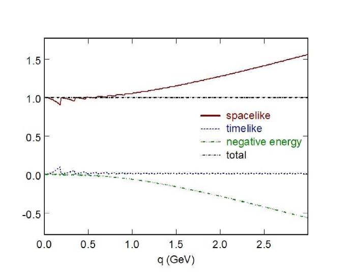
FIG. 1.: Positive energy spacelike, timelike and negative energy contributions to the Coulomb Sum rule from our model.

Since the jaggedness in the spacelike region is associated with the migration of contributions from the timelike region, it is not surprising to see that the complement of this behavior does indeed show up in the timelike contribution. As the momentum transfer increases, the size of the timelike contribution becomes small. The negative energy contribution is smooth and compensates for the over-saturation of the spacelike contribution. This is clearly an artifact of using a one-body wave equation with negative energy contributions.

It should be pointed out here that the small size of the timelike contributions is an essential consequence of using a relativistic wave equation. This can be seen by considering a similar situation where the nonrelativistic oscillator model is used to describe the system. The spacelike and timelike contributions of such a model are shown in Fig. 2. The Schrödinger equation of course has only positive energy solutions. Here the saw-toothed behavior in the spacelike contributions is similar to the relativistic case with the important difference that due to the linear character of the nonrelativistic spectrum (see Fig. 13) the contributions from states entering the spacelike region is not rapid enough to compensate for the fall-off in the form factors. Therefore, with increasing momentum transfer, the size of the spacelike contribution approaches zero with all of the strength appearing in the timelike region.

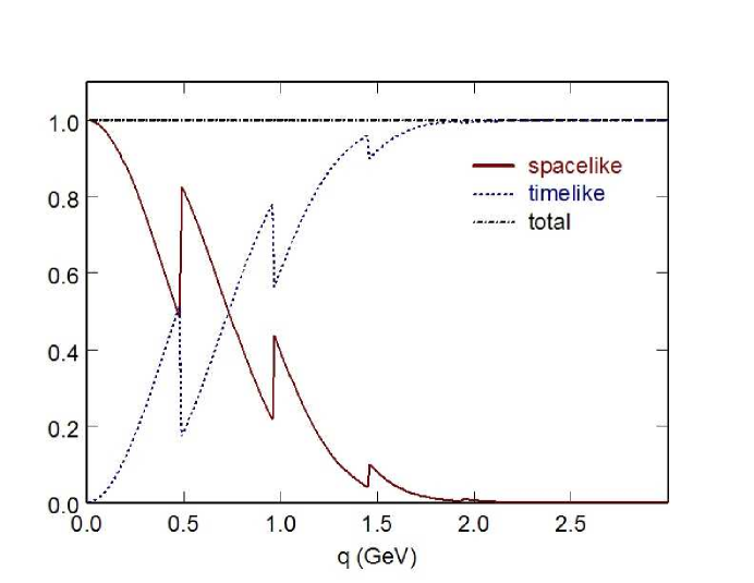
FIG. 2.: Spacelike and timelike contributions to the Coulomb Sum Rule for a nonrelativistic oscillator.

Duality in the sum of the form factors in the spacelike region is related to the Coulomb sum rule. While the concept of duality in the form factors is not clearly related to an observable (in contrast to duality in the structure functions), it still has received attention in the literature [5]. We describe it within our model in appendix A.

This model can be easily extended to the case where both quarks are charged by examining the behavior of the two-body Gross equation in the limit where the mass of one of the particles becomes infinite [16]. The contribution of the infinite mass particle to the structure function is simple and straight forward. Due to its infinite mass, this particle remains stationary for any finite momentum transfer, and it is point-like. This particle therefore contributes only to elastic scattering and has a constant form factor. The structure function can then be written as

$$R_{L}(\vec{q},\nu) = |e_{1}F_{00}(\vec{q})+e_{2}|^{2}$$ (37)

$$+e_{1}^{2}\sum_{N=1}^{\infty}\frac{1}{4\,E_{0}\,E_{N}}|F_{0N}(\vec{q})|^{2}\left[(E_{0}+E_{N})^{2}\delta(\nu+E_{0}-E_{N})\right.$$

$$\qquad\qquad-\left.(E_{0}-E_{N})^{2}\delta(\nu+E_{0}+E_{N})\right]\,$$

The Coulomb Sum can be easily calculated to be

$$S(\vec{q}) = e_{1}^{2}\sum_{N=0}^{\infty}|F_{0N}(\vec{q})|^{2}+e_{2}^{2}+2e_{1}e_{2}\Re F_{00}(\vec{q})$$ (38)

$$= e_{1}^{2}+e_{2}^{2}+2e_{1}e_{2}\Re F_{00}(\vec{q})$$ (39)

So in this case

$${\cal F}(\vec{q})=\Re F_{00}(\vec{q})=F_{00}(\vec{q})\,.$$ (40)

After examining how the apparent contradiction between coherent and incoherent scattering is resolved in a more general framework, we now proceed to investigate duality in our model. The first condition for duality is that one obtains scaling in the structure function calculated solely with resonances, and that the scaling curve thus obtained agrees with the scaling curve obtained in the parton model.

IV The Parton Model

The usual assumption of the parton model is that at large momentum transfers the final state quarks can be treated as though they were free. Examination of the structure functions for large $Q^{2}$ and fixed Bjorken $x$ leads to identification of the scaling functions.

For our simple model, the response functions for excitation of a bound (off-mass-shell) quark to a plane-wave final state can be calculated analytically as

$$R_{L}(\vec{q},\nu) = \frac{(2E_{0}+\nu)^{2}}{4\pi^{\frac{1}{2}}\beta E_{0}|\vec{q}|}\left[\exp{\left(-\frac{y^{2}}{\beta^{2}}\right)}-\exp{\left(-\frac{(y+2|\vec{q}|)^{2}}{\beta^{2}}\right)}\right]$$ (42)

$$\times\left[\theta(\nu+E_{0}-m)-\theta(-\nu-E_{0}-m)\right]$$

and

$$R_{T}(\vec{q},\nu) = \frac{\beta}{2\pi^{\frac{1}{2}}E_{0}|\vec{q}|^{2}}\left[\left(2(y+|\vec{q}|)-\frac{\beta^{2}}{|\vec{q}|}\right)\exp{\left(-\frac{y^{2}}{\beta^{2}}\right)}\right.$$ (45)

$$-\left.\left(2(y+|\vec{q}|)+\frac{\beta^{2}}{|\vec{q}|}\right)\exp{\left(-\frac{(y+2|\vec{q}|)^{2}}{\beta^{2}}\right)}\right]$$

$$\times\left[\theta(\nu+E_{0}-m)-\theta(-\nu-E_{0}-m)\right]$$

where $y=\sqrt{(\nu+E_{0})^{2}-m^{2}}-|\vec{q}|$.

For our model it is not possible to define the scaling variable in terms of the target mass since it is infinite. For this reason we define a new Bjorken variable

$$u_{Bj}=\frac{M}{m}x_{Bj}=\frac{Q^{2}}{2m\nu}$$ (46)

which covers the interval $-\infty<u_{Bj}<\infty$. Using $\nu=\frac{Q^{2}}{2mu_{Bj}}$, and taking the limit $Q^{2}\rightarrow\infty$, the structure functions become

$$R_{L}(Q^{2},u_{Bj})\rightarrow\frac{Q^{2}}{8\pi^{\frac{1}{2}}\beta mE_{0}u_{Bj}}\exp{\left(-\frac{(E_{0}-mu_{Bj})^{2}}{\beta^{2}}\right)}\left[\theta(\frac{Q^{2}}{2mu_{Bj}})-\theta(-\frac{Q^{2}}{2mu_{Bj}})\right]\,,$$ (47)

and

$$R_{T}(Q^{2},u_{Bj})\rightarrow\frac{2\beta mu_{Bj}}{\pi^{\frac{1}{2}}E_{0}Q^{2}}\exp{\left(-\frac{(E_{0}-mu_{Bj})^{2}}{\beta^{2}}\right)}\left[\theta(\frac{Q^{2}}{2mu_{Bj}})-\theta(-\frac{Q^{2}}{2mu_{Bj}})\right]\,.$$ (48)

Since in this limit

$$|\nu|\frac{Q^{4}}{\vec{q}^{4}}\rightarrow\frac{8m^{3}|u_{Bj}|^{3}}{Q^{2}}\mbox{ and }|\nu|\frac{Q^{2}}{2\vec{q}^{2}}\rightarrow m|u_{Bj}|$$ (49)

the structure functions have the limits

$$W_{1}(u_{Bj},Q^{2})\rightarrow F_{1}(u_{Bj})=0$$ (50)

and

$$|\nu|W_{2}(\nu,Q^{2})\rightarrow F_{2}(u_{Bj})=\frac{m^{2}u_{Bj}^{2}}{\pi^{\frac{1}{2}}\beta E_{0}}\exp{\left(-\frac{(E_{0}-mu_{Bj})^{2}}{\beta^{2}}\right)}\,.$$ (51)

Note that the choice of $|\nu|$ in defining $W_{2}$ is necessary to provide a properly normalized scaling function as will be seen below.

Although we have used the Bjorken scaling variable to obtain these results, this will be true for all such variables since all acceptable scaling variables must reduce to the Bjorken scaling variable as $Q^{2}\rightarrow\infty$. Therefore, a more general expression for $F_{2}$ for any scaling variable and any initial state can be written as

$$F_{2}(u)=\frac{m^{2}u^{2}}{4\pi^{2}E_{0}}\int_{|E_{0}-mu|}^{\infty}dp\,pN(p)$$ (52)

where $N(p)$ is the ground state momentum distribution normalized such that

$$\frac{1}{2\pi^{2}}\int_{0}^{\infty}dpp^{2}N(p)=1\,.$$ (53)

After obtaining the scaling curve in the parton model, i.e. the scaling curve for a quark initially bound and then free, we proceed to find an expression for the scaling curve in our model, where the quark makes the transition from the ground stated to an excited bound state.

V Continuum Limit

An interesting feature of our relativistic oscillator model is that the scaling behavior of the model can be determined analytically by making a continuum approximation. The justification for this is that at increasing momentum transfer the contributions to the response functions are dominated by higher energy states. Since the density of states increases with increasing energy, it is reasonable that a continuum approximation should provide a good description of the averaged response for large momentum transfers.

Using (10) and (13) we can write

$$R_{L}(\vec{q},\nu) = \sum_{N=0}^{\infty}\,\Delta N\frac{1}{4E_{0}E_{N}}\,\,\frac{1}{N!}\left(\frac{\vec{q}\,^{2}}{2\beta^{2}}\right)^{N}\exp{(-\frac{\vec{q}\,^{2}}{2\beta^{2}})}$$ (55)

$$\times\left[(E_{N}+E_{0})^{2}\delta(E_{N}-E_{0}-\nu)-(E_{0}-E_{N})^{2}\delta(E_{N}+E_{0}+\nu)\right]$$

where $\Delta N=1$. It is convenient to write

$$E_{N}=\sqrt{p_{N}^{2}+E_{0}^{2}}$$ (56)

where

$$p_{N}^{2}=2\beta^{2}N\,.$$ (57)

¿From this it can be determined that for a variation in $N$,

$$\Delta N=\frac{p_{N}\Delta p_{N}}{\beta^{2}}\,,$$ (58)

and

$$\Delta E_{N}=\frac{p_{N}\Delta p_{N}}{E_{N}}\,.$$ (59)

The longitudinal response function can then be rewritten as

$$R_{L}(\vec{q},\nu) = \frac{1}{4\beta^{2}E_{0}}\sum_{N=0}^{\infty}\,\frac{\Delta E_{n}}{\Gamma\left(1+\frac{E_{N}^{2}-E_{0}^{2}}{2\beta^{2}}\right)}\left(\frac{\vec{q}\,^{2}}{2\beta^{2}}\right)^{\frac{E_{N}^{2}-E_{0}^{2}}{2\beta^{2}}}\exp{(-\frac{\vec{q}\,^{2}}{2\beta^{2}})}$$ (61)

$$\times\left[(E_{N}+E_{0})^{2}\delta(E_{N}-E_{0}-\nu)-(E_{0}-E_{N})^{2}\delta(E_{N}+E_{0}+\nu)\right]\,.$$

This sum can now be approximated by the integral

$$R_{L}(\vec{q},\nu) = \frac{1}{4\beta^{2}E_{0}}\int_{E_{0}}^{\infty}\,\frac{dE}{\Gamma\left(1+\frac{E^{2}-E_{0}^{2}}{2\beta^{2}}\right)}\left(\frac{\vec{q}\,^{2}}{2\beta^{2}}\right)^{\frac{E^{2}-E_{0}^{2}}{2\beta^{2}}}\exp{(-\frac{\vec{q}\,^{2}}{2\beta^{2}})}$$ (63)

$$\times\left[(E+E_{0})^{2}\delta(E-E_{0}-\nu)-(E-E_{0})^{2}\delta(E+E_{0}+\nu)\right]\,$$

which can be trivially evaluated to give

$$R_{L}(\vec{q},\nu)=\frac{(\nu+2E_{0})^{2}\left[\theta(\nu)-\theta(-2E_{0}-\nu)\right]}{4\beta^{2}E_{0}\Gamma\left(1+\frac{(\nu+E_{0})^{2}-E_{0}^{2}}{2\beta^{2}}\right)}\left(\frac{\vec{q}\,^{2}}{2\beta^{2}}\right)^{\frac{(\nu+E_{0})^{2}-E_{0}^{2}}{2\beta^{2}}}\exp{(-\frac{\vec{q}\,^{2}}{2\beta^{2}})}\,.$$ (64)

Similarly, the transverse response becomes

$$R_{T}(\vec{q},\nu)=\frac{(\nu^{2}+2E_{0}\nu)\left[\theta(\nu)-\theta(-2E_{0}-\nu)\right]}{E_{0}\vec{q}^{2}\Gamma\left(1+\frac{(\nu+E_{0})^{2}-E_{0}^{2}}{2\beta^{2}}\right)}\left(\frac{\vec{q}\,^{2}}{2\beta^{2}}\right)^{\frac{(\nu+E_{0})^{2}-E_{0}^{2}}{2\beta^{2}}}\exp{(-\frac{\vec{q}\,^{2}}{2\beta^{2}})}\,.$$ (65)

In the scaling limit the argument of the $\Gamma$ function becomes large, so Stirling’s formula can be used to write the longitudinal response function as

$$R_{L}(\sqrt{Q^{2}+\nu^{2}},\nu) = \frac{(\nu+2E_{0})^{2}}{4\pi^{\frac{1}{2}}\beta E_{0}}\frac{\exp{\left(\frac{\nu^{2}+2E_{0}\nu}{2\beta^{2}}\ln\left(\frac{Q^{2}+\nu^{2}}{\nu^{2}+2E_{0}\nu}\right)-\frac{Q^{2}+\nu^{2}}{2\beta^{2}}+\frac{\nu^{2}+2E_{0}\nu}{2\beta^{2}}\right)}}{\sqrt{\nu^{2}+2E_{0}\nu}}$$ (67)

$$\times\left[\theta(\nu)-\theta(-2E_{0}-\nu)\right]\,.$$

Using

$$\nu=\frac{Q^{2}}{2mu_{Bj}}\,,$$ (68)

and taking the limit $Q^{2}\rightarrow\infty$, the structure functions become

$$R_{L}(Q^{2},u_{Bj})\rightarrow\frac{Q^{2}}{8\pi^{\frac{1}{2}}\beta mE_{0}u_{Bj}}\exp{\left(-\frac{(E_{0}-mu_{Bj})^{2}}{\beta^{2}}\right)}\left[\theta(\frac{Q^{2}}{2mu_{Bj}})-\theta(-\frac{Q^{2}}{2mu_{Bj}})\right]\,,$$ (69)

Similarly,

$$R_{T}(Q^{2},u_{Bj})\rightarrow\frac{2\beta mu_{Bj}}{\pi^{\frac{1}{2}}E_{0}Q^{2}}\exp{\left(-\frac{(E_{0}-mu_{Bj})^{2}}{\beta^{2}}\right)}\left[\theta(\frac{Q^{2}}{2mu_{Bj}})-\theta(-\frac{Q^{2}}{2mu_{Bj}})\right]\,.$$ (70)

Since (69) and (70) are identical to (47) and (48) the model scales to the parton model result. So, even though our model describes a bound quark being excited to resonance states, we do obtain a scaling curve in the Bjorken limit. This, as well as the results presented in [17, 18, 19, 6], show that scaling does not necessarily imply scattering off free constituents, a belief which is encountered widely.

While others [17, 18, 19] have studied the transition from ground state to excited bound states and found scaling in similar models. However, duality is fulfilled only when i) the transition from ground state to excited bound states scales, ii) the transition from ground state to a plane-wave final state scales, and iii) both scaling curves coincide. In this section and the preceding section, we have shown that duality holds explicitly in our model. The numerical approach towards the scaling curve is shown in Fig. 3.

Note that as we explicitly made use of Stirling’s formula in the derivation of the scaling function in the continuum limit, it is clear that for the lower lying resonances, which correspond to lower $N$ values, we will never quite see scaling in the subasymptotic regime. This is of no practical relevance, as these resonances are pushed out to very high values of $u$ for larger $Q^{2}$, and the structure functions practically vanish in this region. This is completely analogous to the fact that for electron scattering from a proton, one always picks up the elastic scattering at $x_{Bj}=1$, independent of $Q^{2}$ - even though the elastic form factor will have fallen off to negligible values at high enough $Q^{2}$.

VI Approach to scaling in the structure functions

After establishing analytically that one of the necessary conditions for duality is fulfilled, namely scaling to the scaling curve obtained from a free quark in the final state, we proceed to investigate the approach to scaling numerically.

We would like to remind the reader that our results should not be compared to the available nucleon data - our model calculations describe a process that might resemble electron scattering from a $B$ meson, which has never been measured. In general, when we consider scattering from a meson target, scaling will set in later than for a baryon target: momentum sharing for higher momenta between fewer constituents is easier, which leads to a slower fall-off of the individual form factors, and to a later onset of scaling. In our situation, where the system is not allowed to decay, we have a somewhat extreme case.

To see duality clearly both experimentally and theoretically, one needs to go beyond the Bjorken scaling variable $x_{Bj}$ and the scaling function ${\cal{S}}_{2Bj}=\nu W_{2}$ that goes with it. This is because in deriving Bjorken’s variable and scaling function, one not only assumes $Q^{2}$ to be larger than any mass scale in the problem, but also that high $Q^{2}$ (pQCD) dynamics controls the interactions. However, duality has its onset in the region of low to moderate $Q^{2}$, and there masses and violations of asymptotic freedom do play a role. Bloom and Gilman used a new, ad hoc scaling variable $\omega^{\prime}$ [1] in an attempt to deal with this fact. In most contemporary data analyses, the Nachtmann variable [21, 20] is used together with ${\cal{S}}_{2Bj}$. Nachtmann’s variable contains the target mass as a scale, but neglects quark masses. For our model, the constituent quark mass (assumed to arise as a result of spontaneous chiral symmetry breaking) is vital at low energy, and a scaling variable that does not make any assumptions about the size of the quark and target masses compared to $Q^{2}$ is desirable. Such a variable was derived more than twenty years ago by Barbieri et al. [22] to take into account the masses of heavy quarks; we use it here given that after spontaneous chiral symmetry breaking the nearly massless light quarks have become massive constituent quarks, calling it $x_{cq}$:

$$x_{cq}=\left\{\begin{array}[]{ll}\frac{1}{2M}\left(\sqrt{\nu^{2}+Q^{2}}-\nu\right)\left(1+\sqrt{1+\frac{4m^{2}}{Q^{2}}}\right)&\mbox{for $\nu>0$}\\ -\frac{1}{2M}\left(\sqrt{\nu^{2}+Q^{2}}+\nu\right)\left(1+\sqrt{1+\frac{4m^{2}}{Q^{2}}}\right)&\mbox{for $\nu<0$}\end{array}\right.\,.$$ (71)

where the definition for negative energy is chosen such that it satisfies the kinematic constraints in this region and reproduces the behavior of $x_{Bj}$ for large $Q^{2}$. The scaling function associated with this variable is given by:

$${\cal{S}}_{2cq}\equiv|\vec{q}|\ W_{2}=\sqrt{\nu^{2}+Q^{2}}\ W_{2}\,.$$ (72)

This scaling function and variable were derived for scalar quarks which are free, but have a momentum distribution. The derivation of a new scaling variable and function for bound quarks will be published elsewhere. Numerically, this scaling variable does not differ very much from the one in Eq. (71). Of course all versions of the scaling variable must converge to $x_{Bj}$ and all versions of the scaling function must converge towards ${\cal{S}}_{Bj}$ for large enough $Q^{2}$. One can also easily verify that in the limit $m\to 0$ one obtains from (71) the Nachtmann scaling variable. In the following, we use the variable $x_{cq}$ and the scaling function ${\cal{S}}_{2cq}$.

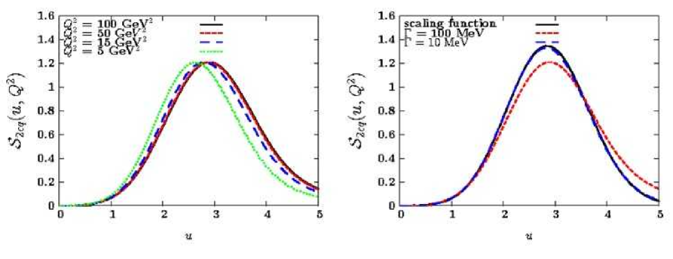
FIG. 3.: The high energy scaling behavior of ${\cal{S}}_{2cq}$ as a function of $u$ for various values of $Q^{2}$. In the left panel, we have used $\Gamma=100$ MeV to give the impression of real resonances even though this large value distorts the scaling curve somewhat. For any width equal to or smaller than this, the distortion is rather innocuous, and for $\Gamma\rightarrow 0$, the structure function approaches the scaling function (solid line) in Eq. (51), as shown in the right hand panel. The structure functions in the left panel are shown for $Q^{2}$ = 100 GeV².

We are now ready to look at scaling and duality in our model. Since the target has mass $M\rightarrow\infty$, it is convenient to rescale the scaling variable $x_{cq}$ by a factor $M/m$:

$$u \equiv {M\over m}\ x_{cq}\ ~{}~{}.$$ (73)

The variable $u$ takes values from 0 to a maximal, $Q^{2}$ dependent value, which can go to infinity. The high energy scaling behavior of the appropriately rescaled structure function ${\cal{S}}_{cq}$ is illustrated in Fig. 3. The structure function has been evaluated using the phenomenologically reasonable parameters $m=0.33$ GeV and $\beta=0.4~{}{\rm GeV}$. To display it in a visually meaningful manner, the energy-dependent $\delta$-function has been smoothed out by introducing an unphysical Breit-Wigner shape with an arbitrary but small width, $\Gamma$, chosen for purposes of illustration:

$$\delta(E_{N}-E_{0}-\nu)\rightarrow\frac{\Gamma}{2\pi}\,\,\frac{f}{(E_{N}-E_{0}-\nu)^{2}+(\Gamma/2)^{2}}\,,$$ (74)

where the factor $f={\pi}/[{\frac{\pi}{2}+\arctan{2(E_{N}-E_{0})\over\Gamma}]}$ ensures that the integral over the $\delta$-function is identical to that over the Breit-Wigner shape. As for the all scalar case discussed in [4], the smearing out of the $\delta$-function in energy with the Breit-Wigner shape leads to a slight widening of the curve and flattening of the peak height. However, when choosing a smaller value for the Breit-Wigner width, these effects disappear, as seen in the right panel of Fig. 3.

Not unexpectedly, the scaling curve we find here, when using photons and electrons with their appropriate spins, differs from the one in the all scalar case both in its final shape and the approach to scaling. Now, we have two terms, the longitudinal and transverse response function, contributing to the structure function $W_{2}$ and therefore to the scaling curve. More importantly, the terms themselves are different and more complicated in the case considered here. The longitudinal part of the structure function contains an additional factor $(E_{0}+E_{N})^{2}$, which was not present in the all scalar case. As shown in section V, the transverse response vanishes like $1/Q^{2}$ in the limit $Q^{2}\rightarrow\infty$, while the longitudinal response grows like $Q^{2}$. This leads to a vanishing of $W_{1}$, and to a $Q^{2}$ independent value for $|\vec{q}|W_{2}$. Even though, from eqs.(16,69,70) it is clear that at lower $Q^{2}$, the transverse contribution to $W_{2}$ will not vanish immediately, therefore making the approach to scaling slower. The effect is rather significant, though, as the contributions of the convection current are very small. They delay scaling slightly for the low $u$ part of the curve. The effect would be more important for contributions of similar size within a certain kinematic range. In our case, the main effect of the transverse contribution is to slightly broaden the curve. For smaller $Q^{2}$, this effect is more pronounced for low values of the scaling variable $u$, as the higher $u$ correspond to lower lying resonances, which have only tiny contributions from the transverse part.

As already mentioned above, for a proton target, the dominant contribution to the transverse response and overall is the magnetization current, which does not contribute for our scalar “quarks”. Note that both the transverse and longitudinal contribution to $W_{2}$ are positive definite. If a dominant contribution in the transverse response is present, it should lead to a different scaling behavior in the structure function $W_{1}$ than in $\nu W_{2}$. For $\nu W_{2}$, the longitudinal term with different $Q^{2}$ behavior will most likely slow the approach to scaling down, as it is going to be of comparable size to the magnetization current contribution at low $Q^{2}$. This is a completely general observation, and one would expect to see faster scaling in $F_{1}$ once the data are available. The same conclusion was reached on a different basis in [5].

The shape of the scaling curve is also different than for the all scalar case. The peak is higher, the curve extends to larger values of the scaling variable, and for $u\rightarrow 0$, the scaling function actually vanishes now, as expected from a valence quark distribution, even though we do not find a behavior $\propto\sqrt{u}$ as seen for proton targets. However, we cannot expect to reproduce the correct distribution function for quarks in our simple model with scalar “quarks”.

From the explicit expression for the scaling curve, it is clear that it depends both on the binding strength $\beta$ of the harmonic oscillator, and on the quark mass. It peaks at $u_{peak}=(E_{0}+\sqrt{E_{0}^{2}+\beta^{2}})/2m$, slightly above the value $u_{peak}^{scalar}=\frac{E_{0}}{m}$ which we found for the all scalar case. Naively, for a target of mass $M$ made up of non-interacting quarks of mass $m_{q}$, one expects a spike at $x_{Bj}=\frac{m_{q}}{M}$. In our case, the role of the mass of the quark $m_{q}$ is played by the ground state energy $E_{0}$, which appears everywhere (e.g. in flux factors, normalization) where one would have the mass in the free particle case. As our variable is rescaled with the factor $\frac{M}{m}$, we expect $u_{peak}\approx\frac{E_{0}}{m}$. It is interesting to note that this value receives a slight binding correction due to the conserved current employed here. We note that for weaker binding, the peak gets narrower and its position slides towards $u\approx 1$. As expected, in the limit of a free particle, $\beta\rightarrow 0$, we do obtain a spike of infinite height at $u=1$ [in this limit, the scaling function becomes $\delta(u)/(mE_{0})$].

VII Moments and further Sum Rules

Now, we will discuss global duality, where the term global implies that we consider an average/integral over many resonances, which is compared with the corresponding integral over the scaling curve.

Local duality implies that we compare the contribution of one single resonance or just a few resonances with the scaling result, i.e. with the free quark result. This will be discussed in section VIII. The concept of local duality is taken to its extreme when one focuses not just on one single resonance, but on one point only of the contribution of the single resonance, as it was done first by Bloom and Gilman [1], when they compared the peak value of a single resonance with the value of the scaling curve. This version of duality has been investigated in Ref. [23]. As this ratio would depend strongly on the Breit-Wigner width we use to smooth out the $\delta$-functions, it is not appropriate to consider it in this paper.

Global duality was first quantified by Bloom and Gilman [1] in the form of finite energy sum rules, where the integral over the scaling curve was compared to the integral over the resonance contribution. The integration range in both cases comprises the region of the scaling variable $\omega^{\prime}$ or $\nu$, respectively, which corresponds to the resonance region, defined as having an invariant mass $W<2$ GeV:

$$\frac{2M_{N}}{Q^{2}}\int_{0}^{\nu_{m}}d\nu\nu W_{2}(\nu,Q^{2})=\int_{1}^{1+W_{m}^{2}/Q^{2}}d\omega^{\prime}\nu W_{2}(\omega^{\prime})\,,$$ (75)

where $W_{m}\approx 2$ GeV, and $\nu_{m}=\frac{W_{m}^{2}-M_{N}^{2}+Q^{2}}{2M_{N}}$. Here, $M_{N}$ denotes the mass of the nucleon target. The agreement between the left and right hand side of this equation is better than $10~{}\%$; for the larger values of Q², starting around Q${}^{2}\approx 2$ GeV², the agreement is quite impressive: $2\%$ or better.

While it certainly would be desirable to calculate the same finite energy sum rule in our model, there is a practical problem and a philosophical problem. Firstly, in our model, we deal with an infinitely heavy system, so that in principle, the invariant mass $W$ of the final state is always infinity. Even if we could define a reasonable substitute for the invariant mass of the final state, picking an integration limit is a problem in principle: for our model, the scaling curve consists solely of resonance contributions, even though they cannot be resolved and form a smooth curve. So, any distinction between “resonance region” and “continuum” or “multiparticle final states” is artificial. The conventional definition of “resonance region” as the region where $W<2$ GeV means the region where the resonances are prominent and dominant. However, it does not mean that for $W>2$ GeV, there are no resonances present, and it also does not mean that for $W<2$ GeV, i.e. in the resonance region, there are no non-resonant contributions at all. Experimentally, there is background for $W<2$ GeV, and there are resonances for $W>2$ GeV, e.g. several $N^{*}$ and $\Delta$ resonances. Also from a theoretical point of view, it is obvious that resonances which decay by creation of a quark-antiquark pair in the final state must be accompanied by a corresponding non-resonant production mechanism, where the pair creation takes place in the initial state, and the photon interacts with the preformed meson.

Since the distinction between a “resonance region” and a “continuum region” has its problems, we utilize the moments of the scaling function ${\mathcal{S}}_{cq}$, where the integration range comprises the whole interval of the scaling variable. The physical information contained in the finite energy sum rule and the moments $M_{n}$ is the same. The moments of a scaling function ${\mathcal{S}}(Q^{2},x)$ with a scaling variable $x$ are defined as

$$M_{n}(Q^{2})=\int_{0}^{x_{max}}dx\,\,x^{n-2}\,{\mathcal{S}}_{2}(Q^{2},x)\,.$$ (76)

Here, in contrast to [24], we do not include the unphysical region $]x_{max},1]$ in the integration interval. It is obvious that higher moments, i.e. $n=4,6,\dots$, tend to emphasize the resonance region, as for fixed Q², the resonances are found at large $x$. The values of the moments decrease with increasing $n$. In our case, we change to $u$-type scaling variables, see Eq. 73, so that

$$M_{n}^{u-based}(Q^{2})=\int_{0}^{u_{\rm max}}du\,\,u^{n-2}\,{\mathcal{S}}_{2}(Q^{2},u)\,,$$ (77)

where $u_{\rm max}$ corresponds to the maximum value of $u$ which is kinematically accessible at a given $Q^{2}$. By changing from $x$ to $u$ scaling variables, we change the upper integration limit from a value equal to or lower than 1 to a value considerably larger than 1 for Q${}^{2}>1-2$ GeV². This means that our higher moments will emphasize the low-lying resonances even more than the conventional, $x$-based moments. Also, the higher moments will be larger than the moments with small $n$.

Evaluating the moments of the structure function (72) explicitly one has

$$M_{n}(Q^{2}) = \left(\frac{r}{2m}\right)^{n-1}\,\sum_{N=0}^{\infty}\,\left(\sqrt{\nu_{N}^{2}+Q^{2}}-\nu_{N}\right)^{n-1}\,\,\frac{E_{0}}{E_{N}}\,\left|F_{0N}\left(\sqrt{\nu_{N}^{2}+Q^{2}}\right)\right|^{2}~{}~{}$$ (79)

$$\qquad\qquad\times\left[\frac{Q^{4}}{q_{N}^{4}}(E_{0}+E_{N})^{2}+4N\alpha\frac{Q^{2}}{q_{N}^{4}}\right]\,,$$

with $r\equiv 1+\sqrt{1+4m^{2}/Q^{2}}$, and $\nu_{N}=E_{N}-E_{0}$ and $q_{N}=\sqrt{Q^{2}+\nu_{N}^{2}}$.

The elastic contribution is given by

$$M_{n}^{elastic}(Q^{2})=\left(\frac{r}{2m}\right)^{n-1}\,|Q|^{n-1}\,\exp(-\frac{Q^{2}}{2\beta^{2}})$$ (80)

Note that for vanishing four-momentum transfer $Q^{2}$, all moments take the value $1$, independent of $n$.

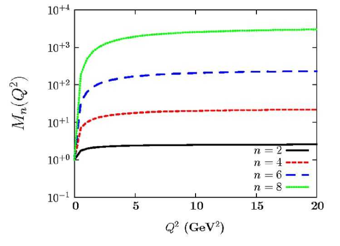
FIG. 4.: The lowest moments $M_{n}$ as a function of $Q^{2}$.

In Fig. 4, we show the moments for $n=2,4,6,8$, which were obtained by integrating over the positive energy states only. One can see clearly that all moments flatten out, even though they did not quite reach their asymptotic value at the highest $Q^{2}$ value shown. The lowest moment $M_{n}$, is within 9 % of its asymptotic value at $Q^{2}=5$ GeV², and within   % of its asymptotic value at $Q^{2}=20$ GeV². As expected, the higher moments, which by construction get more contributions from the lower lying resonances, need higher $Q^{2}$ values in order to reach their asymptotic values. For $M_{6}$, we find that it has reached 64 % of its asymptotic value at $Q^{2}=5$ GeV², and 88 % of its asymptotic value at $Q^{2}=20$ GeV². From these numbers, we can see that even though scaling does not set in for $Q^{2}<50$ GeV², the asymptotic values at least of the lower moments are reached much earlier. This reflects the fact that ${\cal{S}}_{cq}(u,Q^{2})$ approaches the scaling curve by shifting towards higher $u$, not by approaching it from below or above.

Since the continuum approximation provides a relatively simple analytic expression for the structure functions, it is possible to use this to study certain properties of the moments. First, however, it is necessary to determine the validity of this approximation for the calculation of moments. Figure 5 shows calculations of the first three moments $M_{0}$, $M_{1}$ and $M_{2}$.

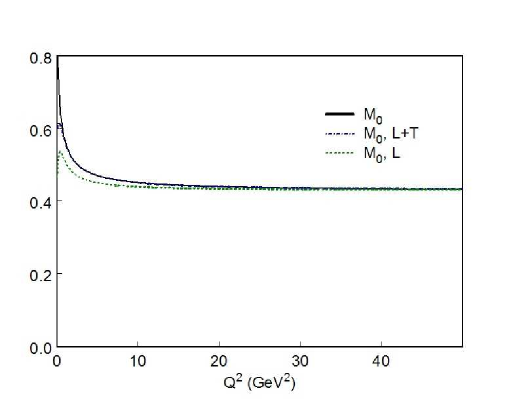
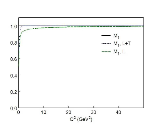
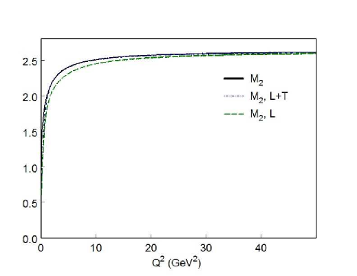
FIG. 5.: The first three moments, $M_{0}$, $M_{1}$, and $M_{2}$. The solid line shows the exact result calculated according to Eq. 79. The dash-dotted lines show the moment calculated in the continuum approximation, the dotted curves show the purely longitudinal contribution to the moment in the continuum approximation. Inclusion of the transverse contributions improves convergence of the moments to their asymptotic values.

In each panel the solid line represents the exact calculation according to (79). The dash-dotted curve is a calculation of the continuum approximation with both longitudinal and transverse contributions, while the dashed curve includes only the longitudinal contribution. Note that the continuum approximation works very well down to a couple of GeV². Note also that while the inclusion of the transverse contribution slows convergence to the asymptotic value for $M_{0}$ it improves convergence for the higher moments.

The continuum approximation can then be used to obtain an expansion of the moments in powers of $1/Q^{2}$ reminiscent of the operator product expansion (OPE) series,

$$M_{n}^{2k}(Q^{2})=\sum_{i=0}^{k}\frac{c^{2i}_{n}}{Q^{2i}}\,.$$ (81)

Note that we do not have any gluons in our model, and thus no radiative corrections. The expansion coefficients $c^{2i}_{n}$ correspond to the non-perturbative matrix elements of higher twist operators in the OPE. Since this is an asymptotic series, the expansion will fail at low $Q^{2}$ with the point at which the series diverges being dependent upon the order of the series. The expansion coefficients for the five lowest moments are shown in Table I. Contributions to the coefficients from transverse and longitudinal responses are shown along with the total.

TABLE I.: Leading coefficients of the expansion of the moments in $1/Q^{2}$

		$c^{0}_{n}$	$c^{2}_{n}$	$c^{4}_{n}$	$c^{6}_{n}$
$M_{0}$	L	0.42859	0.20760	-0.26022	0.13530
	T	0.00000	0.13715	-0.19201	0.19056
	total	0.42859	0.34475	-0.45223	0.32586
$M_{1}$	L	1.00037	-0.32052	0.95887	-2.83879
	T	0.00000	0.32012	-0.95870	2.83881
	total	1.00037	-0.00039	0.00017	0.00002
$M_{2}$	L	2.64117	-2.37461	5.53199	-14.8231
	T	0.00000	0.84518	-3.22720	10.6710
	total	2.64117	-1.52944	2.30479	-4.1521
$M_{3}$	L	7.6117	-11.1960	26.8417	-71.9074
	T	0.0000	2.4357	-11.2072	40.7982
	total	7.6117	-8.7603	15.6345	-31.1092
$M_{4}$	L	23.5214	-47.6636	122.363	-336.920
	T	0.0000	7.5268	-40.233	159.245
	total	23.5214	-40.1368	82.130	-177.675

The obvious feature of these coefficients is that they are not in general small nor do they show any obvious convergence. The reason for this can be seen from Fig. 6. Here the exact result is shown as a solid line and is compared to the expansion with from one to four terms for both $M_{0}$ and $M_{4}$.

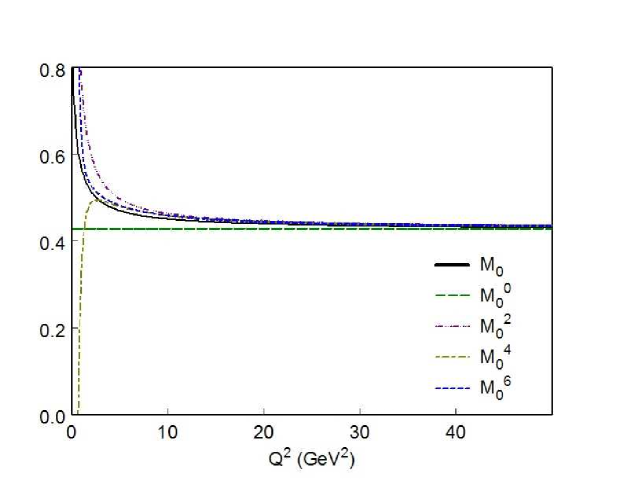
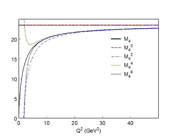
FIG. 6.: Comparison of moments to the expansion of the continuum approximation in $1/Q^{2}$.

Since the moments all have a finite value at $Q^{2}=0$, the function cannot be analytic in $1/Q^{2}$. Any expansion in this variable to a finite number of terms will at some point diverge, either above or below the correct result. Using an additional term to extend the approximation to lower $Q^{2}$ must require that the coefficient of this term be of opposite sign to the preceding term, leading to an alternating series. Higher moments have the curvature toward the finite result occurring at increasing values of $Q^{2}$. This requires that the size of the coefficients for the higher terms in the series must also be increasing. This shows that the global duality observed in our model is the result of a delicate cancellation between many “higher twist” terms. However, while it is fascinating to speculate if duality in Nature is realized by small higher order expansion coefficients or by cancellations, our model is too simple to allow us to draw any conclusions about this. In fact, results presented in [25] indicate that the expansion coefficients have the same sign. One may hope that the building of more realistic models will allow us to gain a better insight into this question in the future.

The relation asymptotic behavior of the moments to sum rules can also be addressed in this model. Consider the moments of $F_{2}(u)$

$${\cal M}_{n}\equiv\int_{-\infty}^{\infty}du\,u^{n-2}F_{2}(u)\,,$$ (82)

where the integral starts at $-\infty$ to include contributions from negative energy states as in the Coulomb Sum Rule. Using (52) this becomes

$${\cal M}_{n} = \frac{m^{2}}{4\pi^{2}E_{0}}\int_{-\infty}^{\infty}du\,u^{n}\int_{|E_{0}-mu|}^{\infty}dp\,p\,N(p)=\frac{m^{2}}{4\pi^{2}E_{0}}\int_{0}^{\infty}dp\,p\,N(p)\int_{\frac{E_{0}-p}{m}}^{\frac{E_{0}+p}{m}}du\,u^{n}$$ (83)

$$= \frac{m^{2}}{4\pi^{2}E_{0}}\int_{0}^{\infty}dp\,p\,N(p)\frac{1}{n+1}\left[\left(\frac{E_{0}+p}{m}\right)^{n+1}-\left(\frac{E_{0}-p}{m}\right)^{n+1}\right]$$ (84)

The two lowest moments

$${\cal M}_{0}=\frac{m}{2\pi^{2}E_{0}}\int_{0}^{\infty}dp\,p^{2}\,N(p)=\frac{m}{E_{0}}=0.43002$$ (85)

and

$${\cal M}_{1}=\frac{1}{2\pi^{2}}\int_{0}^{\infty}dp\,p^{2}\,N(p)=1$$ (86)

are proportional to the normalization integral of the momentum distribution. Comparing these to the corresponding values of $c^{0}_{0}$ and $c^{0}_{1}$ in Table I shows that the contributions from negative energy states are small. Note also that for a spin-1/2 constituent the expression corresponding to (52) have a leading factor of $u$ rather than $u^{2}$ as in this case. So the sum rules would be associated with $M_{1}$ and $M_{2}$ as expected.

VIII The low Q² Region

After studying the scaling behavior of our model at high Q² and the moments over a range of four-momentum transfers, we now discuss the behavior at low Q². In this region, resonances are dominant for a wide range in the scaling variable.

Before discussing the numerical results, a remark on the kinematics is in order. For a fixed resonance in inclusive electron scattering from the nucleon, its position in terms of Bjorken’s scaling variable is given by $x_{res}=\frac{Q^{2}}{W_{res}^{2}-M_{N}^{2}+Q^{2}}$. This means that for higher Q², the resonance position moves towards higher values of $x_{Bj}$, and for very large Q², $x_{Bj}\rightarrow 1$. In our case, the maximal value of the scaling variable $u$ is larger than 1, and for very large Q², the resonances move out to very large values of $u$, where their contribution is extremely small.

If local duality holds, we expect the resonance curve to oscillate around the scaling curve and to average to it, once Q² is large enough. In Bloom-Gilman duality, the finite energy sum rule gets within 5 % for Q${}^{2}\geq$ 1.75 GeV². For lower Q², the resonances approach the scaling curve from below. In our case, we have the onset of scaling for larger values of Q² than observed in Nature. This is not unexpected, as we consider an infinitely heavy meson as target, and assume that this meson is made up of scalar quarks. For this reason, our cross section for photon exchange for large Q² is dominated by the longitudinal part, and the transverse part, comprising solely the convection current, is very small. In Nature, for spin $1/2$ quarks, we have the magnetization current, which is the dominant component of the cross section, and which therefore determines the scaling behavior. So we cannot expect our model calculation to show the same behavior as experimental data for the same values of the four-momentum transfer.

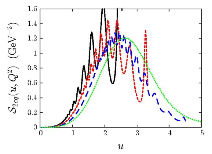
FIG. 7.: The low $Q^{2}$ behavior of ${\cal{S}}_{2cq}(u,Q^{2})$ as a function of $u$ for various values of $Q^{2}$. The solid curve shows $Q^{2}$ = 0.5 GeV², the short-dashed curve shows $Q^{2}$ = 1 GeV², the long-dahsed curve shows $Q^{2}$ = 2 GeV², and the dotted curve shows $Q^{2}$ = 50 GeV².

In discussing local duality and resonances, the smoothing method used becomes important. The visual appearance of “resonances” depends on the chosen smoothing method: a bumpy structure is seen only when a Breit-Wigner shape is inserted for the energy $\delta$-function. It also depends on the width chosen in the Breit-Wigner smoothing method. For a smaller width, the resonances are visible for higher Q². Depending on the width of the Breit-Wigner, e.g. for $\Gamma$ = 100 MeV, we do not see any resonances for Q² = 5 GeV², even though this value of Q² is below the scaling region. In this paper, the working definition of local duality which we use is “resonance curves oscillating around the scaling curve”. At some point, when considering more realistic models, it may be useful and necessary to introduce a sharper, more quantitative definition. However, at this stage, we are interested more in qualitative results, and do not intend to quantify how well exactly local duality works for our simple model.

In Fig. 7, we show our results for the scaling function ${\cal{S}}_{2cq}(u,Q^{2})$ for various low values of $Q^{2}$. The $\delta$-function in the energy has been smoothed out using the Breit-Wigner method, with a width of $\Gamma=100$ MeV. For visual purposes, we have assigned a small width to the elastic peak, too. One can see clearly from the figure that the resonances move out towards higher $u$ with increasing Q², as dictated by kinematics. While the elastic peak is rather prominent for Q² = 0.5 GeV² and Q² = 1.0 GeV², it becomes negligible for Q${}^{2}\geq$ 2.0 GeV². This is the phenomenon we have observed already when studying the moments: the elastic contribution there vanishes rapidly with increasing Q².

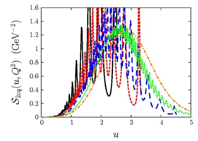
FIG. 8.: The low $Q^{2}$ behavior of ${\cal{S}}_{cq}(u,Q^{2})$ as a function of $u$ for various values of $Q^{2}$. The Breit-Wigner width chosen to smooth out the energy $\delta$-functions is $\Gamma=50MeV$. The solid curve shows $Q^{2}$ = 0.5 GeV², the short-dashed curve shows $Q^{2}$ = 1 GeV², the long-dashed curve shows $Q^{2}$ = 2 GeV², the dotted curve shows $Q^{2}$ = 5 GeV², and the dash-dotted curve shows $Q^{2}$ = 50 GeV².

As already observed while studying the moments in the previous section, the approach to scaling when using a virtual photon is slower than for the all-scalar case discussed in [4]. It is clear that one needs to reach fairly large values of $Q^{2}$ before the “resonance curve” averages with good accuracy to the scaling function. Indeed, with our choice of Breit-Wigner width, this happens only when the bumps have already disappeared, i.e. for $Q^{2}\geq 5$ GeV².

In order to illustrate this point, we have included Fig. 8, where we used a value of $\Gamma=50$ MeV to smooth out the energy $\delta$-function. The curves are more jagged than for the larger width, and the $Q^{2}=5$ GeV² curve still shows plenty of resonance structure.

Overall, we find that the onset of local duality is definitely slower than for the all scalar case, which is what one expects due to the additional structure in the more realistic case discussed in this paper.

IX Summary and Outlook

We have presented a simple, quantum-mechanical model which allows us to obtain the qualitative features of Bloom-Gilman duality. The model assumptions we made are very basic: we assumed relativistic, confined valence scalar quarks, and treated the hadrons in the infinitely narrow resonance approximation. To simplify the situation further, we did not consider a three quark “nucleon” target, but a target composed of an infinitely heavy antiquark and a light quark. In contrast to [4] where all particles involved in the reaction - electrons, photons and quarks - were considered to be scalar, we only use scalar quarks in this paper. This makes the present model more realistic - in particular, we were able to use a conserved current here. However, there is still much work to be done in modelling. The goal of our model calculations is to gain qualitative insight into duality, its applicability and accuracy in various kinematic regions, not to quantitatively describe any data. In the future, we plan to describe more realistic situations in our model. Note that our assumptions are very basic and general, so that we will be able to extend our model in a straightforward manner.

There are several conditions that must be fulfilled in order to see duality. In this paper, we put a special emphasis on three of these conditions: we demonstrated how the transition from coherent scattering at low Q² to incoherent scattering at high Q² takes place, we highlighted the role of relativity by considering the contributions to the Coulomb sum rule in a relativistic framework and a non-relativistic framework, and we gave an analytic proof for the equality of the scaling curve in our model and the parton model result.

Quark-hadron duality is not only very interesting in itself, it also opens the door to very useful applications: duality relates the resonance region data to data from the deep inelastic region. If duality is understood well enough, and if the correct procedures for the averaging of the resonance data and the attendant errors are established, we may exploit duality to gather information in previously unreachable regimes. The investigation of polarized structure functions in the high Bjorken-x region, $x_{Bj}\rightarrow 1$, is a major part of the experimental program at Jefferson Lab [26, 9]. Even without knowing details about the correct averaging procedures, it is clear from the experimental results and our investigation of duality that the conventional, sharp distinction between the “resonance region”, corresponding to an invariant mass $W<2$ GeV, and the “deep inelastic region” where $W>2$ GeV, is entirely artificial.

While quark-hadron duality has been investigated by theorists before, modelling duality is an important new step in our way to a thorough understanding of this phenomenon. In the literature, one often finds the phrase that duality has been explained in terms of QCD by DeRujula, Georgi, and Politzer [24]. What was stated in their paper is that at moderate $Q^{2}$, the higher twist corrections to the lower moments of the structure function are small. The higher twist corrections arise due to initial and final state interactions of the quarks and gluons. Hence, the average value of the structure function at moderate $Q^{2}$ is not very different from its value in the scaling region. While all this is true, the statement is merely a rephrasing of the experimentally observed fact that the resonance curve averages to the scaling curve in terms of the language of the operator product expansion (OPE). However, the operator product expansion does not explain why a certain correction is small or why there are cancellations - the expansion coefficients which determine this behavior are not predicted in the OPE. The ultimate answer to this question might come from a numerical solution of QCD on the lattice, but an understanding of the physical mechanism that leads to the small values of the expansion coefficient in the framework of a model is highly desirable. Also, the OPE will break down for very low $Q^{2}$. Duality was experimentally observed [2] to hold for $Q^{2}$ as low as 0.5 GeV² - a region where the validity of the OPE is questionable. In our analysis of the moments and their expansion coefficients, it became clear that a rigid application of the OPE at very low Q² will inevitably lead to large, alternating expansion coefficients.

The constant resonance to background ratio aspect of duality was addressed in several papers by Carlson and Mukhopadhyay [23]. They used counting rules to find the $Q^{2}$ dependence of the form factors of the resonances in the Breit frame, and compared them to the behavior of the scaling curve for large $x_{Bj}$ and to the behavior of the background in the same region. From these considerations, they could explain the constant ratio, provided the $Q^{2}$-independent coefficients of the helicity amplitudes were not anomalously small, as in the case of the $\Delta$ resonance, for which the ratio vanishes. Still, there is no explanation why the coefficient is small in one case and not in others, and there exist several models with contradictory predictions.

The preceding observations clearly show the need for modelling. Even though one may obtain expansion coefficients from calculations on the lattice, an understanding of the underlying physical mechanisms will most likely be gained only by considering models like ours. One great advantage of a purely analytical model like the one presented here is that explicit derivations of key quantities like the scaling function are feasible. The proof that the scaling function obtained for the transition from a bound quark to an excited bound quark is the same as the scaling function for the transition from a bound quark to a free quark was given here for a linear potential, which is the relativistic analog of a harmonic oscillator. It is desirable to extend the investigation to other types of potential, and to find a proof that applies to a general class of potentials. In a recent publication, [6], numerical methods were applied to study the responses of a massless quark, and a disagreement between results with and without final state interactions were observed. This is in contrast to our findings, and it is important to understand the reasons for these differences.

The experimental data at very low Q² still average to one single curve independent of their Q² [2]. However, this is not duality in the sense defined in this paper because this curve differs from the scaling curve. To investigate this interesting observation, one must go beyond the model presented here, which contains valence quarks only, and therefore must produce a valence-like shape. However, introducing sea quarks and modeling the decay of the excited resonances, along with the corresponding non-resonant production mechanisms from sea quark pairs, might shed considerable light on this issue.

A Duality in the Excitation Form Factors

In this appendix, we proceed to study duality in the excitation form factor $F_{0,N}(\vec{q}^{2})$. While this duality is not directly related to an observable like the structure functions or response functions, it exhibits duality very clearly. Duality in the form factors has recently received some attention in [5].

The duality prediction is that it should not matter if we describe the process in question in a perturbative QCD picture, involving only a free quark, or in a hadronic picture with resonances. The form factor for a hypothetical free quark is just 1, as it does not have any structure. In the hadronic picture, we have inclusive electron scattering where we can excite all resonances – as the final hadronic state is not observed, we have to sum over the resonances incoherently. So we have to compare $\sum_{N}|F_{0,N}(\vec{q}\,^{2})|^{2}$ to 1. Fig. 9 shows single form factors for the lowest resonances, the elastic peak and inelastic excitations up to N = 5. All form factors look qualitatively similar, except for the N=0 elastic form factor, which starts at 1 for $|\vec{q}|=0$. In general, the form factors increase in width and decrease in height with increasing N.

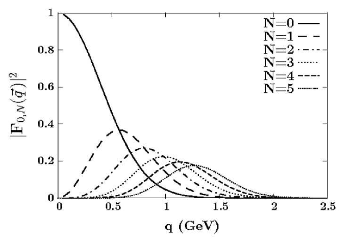
FIG. 9.: The excitation form factor squared, $|F_{0N}(\vec{q}\,)|^{2}$ for the lowest excitations, N = 0 to N = 5, and $\beta=0.4$ GeV.

Using our previous expression for the form factor, eq. (13), we find for the sum up to a certain value $N_{max}$

$$\sum_{N=0}^{N_{max}}|F_{0N}(\vec{q}\,)|^{2}=\exp{(-\frac{\vec{q}\,^{2}}{2\beta^{2}})}\sum_{N=0}^{N_{max}}\frac{1}{N!}\left(\frac{\vec{q}\,^{2}}{2\beta^{2}}\right)^{N}\,,$$ (A1)

and it is obvious that

$$\sum_{N=0}^{N_{max}}|F_{0N}(\vec{q}\,)|^{2}=1\,\,\mbox{if}\,\,\,N_{max}\rightarrow\infty\,,$$ (A2)

as mentioned when discussing the Coulomb sum rule. However, we are limited in the maximal value of $N_{max}$ not by technical problems, but by a physical constraint: we are considering electron scattering, i.e. space-like kinematics, and therefore we must fulfill the condition

$$Q^{2}>0\Leftrightarrow|\vec{q}|>\nu=E_{N}-E_{0}\,,$$ (A3)

so that for fixed three-momentum transfer $|\vec{q}|$, we find a limit on the value of N. The form factor sums are shown in Fig. 10 for various values of the oscillator parameter $\beta$. Larger values of $\beta$ indicate a stronger binding.

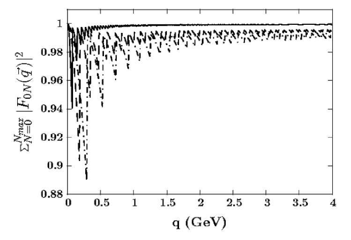
FIG. 10.: The sum over the excitation form factors squared, for $\beta=0.2$ GeV (solid line), $\beta~{}=~{}0.4$ GeV (dashed line), and $\beta=0.6$ GeV (dash-dotted line).

The spiky character of the curves stems from the fact that the form factors for the N-th state are only allowed to contribute to the sum if $|\vec{q}|>\nu_{N}$, where $\nu_{N}:=E_{N}-E_{0}$. Therefore, the sum jumps up whenever another threshold is crossed. This effect can be observed best for the strongest binding, $\beta=0.6$ GeV, as the gaps between the energy levels are largest in this case. With increasing value of the three-momentum transfer, more and more resonance states can be excited and contribute to the sum: the spikes subside and the average value of the sum gets fairly close to 1. The curve for the weakest binding, $\beta=0.2$ GeV, becomes almost smooth and takes on a value of 0.9994, i.e. duality is violated by less than 0.06 %. For $\beta=0.4$ GeV, the sum reaches 0.995, so duality is violated only by 0.5 %. Even for the strongest binding, $\beta=0.6$ GeV, the duality prediction is fulfilled within 1%. Here, we see a typical feature of duality, the need for many resonances to contribute in order to reproduce the behavior of a free quark. At low $|\vec{q}|$, where only a few resonances can contribute, the deviations from 1 are larger. The fact that duality is fulfilled best for weak binding is what we expect: a quark that is bound very lightly and then receives a hard momentum transfer behaves essentially as if it was free. If the binding gets stronger, the situation gets more non-perturbative, and duality does not work as well.

The duality as seen in the form factors is reminiscent of duality in the decay rates of the semileptonic decay of heavy quarks [11, 27]. There, in the limit of infinite masses of the $b$ and $c$ quarks, the loss of strength in the elastic channel is compensated for by the increase in the inelastic decay channels. Once one considers heavy, but not infinitely heavy, quark masses, one obtains a jagged structure, with peaks getting close to the free quark limit, quite similar to what we observe when considering the Coulomb Sum Rule and the excitation form factors.

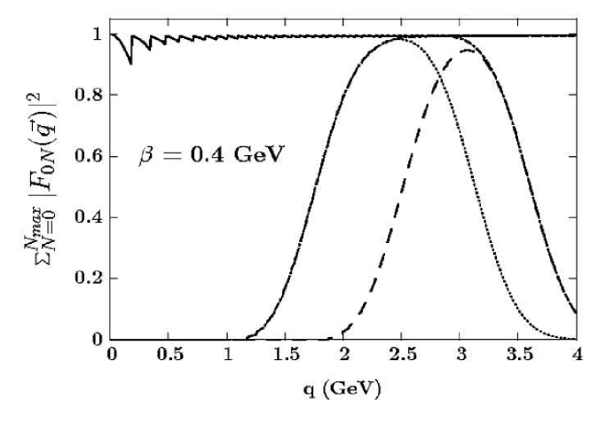
FIG. 11.: The sum over the excitation form factors squared $|F_{0,N}(\vec{q}^{2})|^{2}$ for $\beta=0.4$ GeV. The solid line shows the sum over all allowed N, the dash-dotted line shows the sum from N = 10 to N = 40, the dotted line shows the sum from N = 10 to N = 30, and the dashed line shows the sum from N = 20 to N = 40.

Let us consider the number of resonances needed in more detail, so that we can draw further conclusions on the kind of duality we are observing here. In the calculations presented in Fig. 10, we summed up to the highest allowed N, N_max, which is quite large in general. In Fig. 11, we present the full curve, and three curves where we summed over a limited number of resonances only, namely from N = 10 to N = 40 (dash-dotted line), N = 10 to N = 30 (dotted line) and N = 20 to N = 40 (dashed line). One can see that for a small interval in three-momentum transfer of $\vec{q}=2.6$ GeV - $3.0$ GeV, it is sufficient to include only resonances from N = 10 to N = 40 in order to reproduce the full, unrestricted curve. One also sees from the dotted line that for lower three-momentum transfer, the inclusion of just the twenty resonances from N = 10 to N = 30 suffices to get close to the full curve $\vec{q}=2.6$ GeV, while the same number of resonances does not suffice to approximate the full curve at a slightly higher value of $|\vec{q}|$ (see the dashed line).

So, while it is clear that the “degrees of freedom duality” holds very nicely over the whole kinematic range, we see that duality - the truncated version - does not hold as well: we do need a certain number of resonances to obtain duality in a limited kinematic interval, and this number increases when we increase the three-momentum transfer.

B The Role of Relativity

We have stressed the importance of relativity before, and while it is quite obvious that one needs to include it for GeV momentum transfers to light quarks, it is instructive to see how relativity works for the form factors. In order to illustrate this point, we show the sum of the excitation form factors squared calculated for the non-relativistic harmonic oscillator potential in Fig. 12. As mentioned in section II, the wave functions, and therefore the form factors, are the same. The difference lies in the energy spectrum.

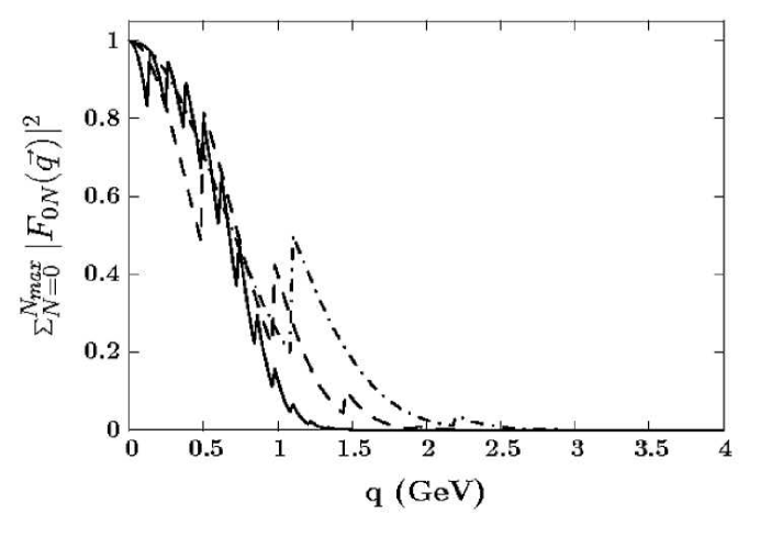
FIG. 12.: The sum over the excitation form factors squared for the non-relativistic case, for $\beta=0.2$ GeV (solid line), $\beta=0.4$ GeV (dashed line), and $\beta=0.6$ GeV (dash-dotted line). Note that the scale differs from the scale in Fig. 10.

Obviously, duality in the non-relativistic case does not work at all: the curves start out at 1, as the elastic form factor for $|\vec{q}|=0$ is 1, but then fall off immediately. Whenever a new threshold opens, the additional contribution is not sufficient to compensate the fall-off of the other form factors: they do not contribute at their maximum value, but only with the “high $|\vec{q}|$” side of the peak, where the form factor drops quickly, see Fig. 9. In the non-relativistic case, the spacing between the energy levels is wider than in the relativistic case, where the levels shrink together. This means that considerably fewer resonances are allowed to contribute at the same, fixed $|\vec{q}|$, and therefore the resulting sum is much smaller and duality is violated. To clarify this point, we show a comparison of energy levels in Fig. 13.

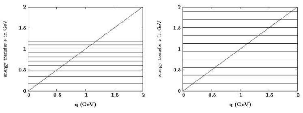
FIG. 13.: The first eleven energy transfers $\nu$ for the relativistic case with $\beta=0.4$ GeV (left panel) and for the non-relativistic case with $\beta=0.25$ GeV (right panel). The diagonal line in both panels indicates the photopoint, i.e. $|\vec{q}|=\nu$. All energy transfers below this line are allowed in the space-like region.

In the left panel, we show the energy transfers $\nu$ for the first eleven energy levels (elastic and the first ten resonances) of a relativistic harmonic oscillator with $\beta=0.4$ GeV. The diagonal line marks the photopoint, $|\vec{q}|=\nu$. This means that for a given $|\vec{q}|$, all the energy transfers below that line are in the space-like region and therefore allowed. E.g., in the relativistic case for $|\vec{q}|=1$ GeV, nine resonances (counting the elastic) can be excited. The right panel of Fig. 13 shows the energy transfers $\nu$ for the energy levels of a non-relativistic harmonic oscillator with $\beta=0.25$ GeV. We chose the $\beta$ for the non-relativistic oscillator in order to reproduce the energy splitting between the ground state and the first excited state of the relativistic case. One clearly sees that fewer resonances can contribute here, e.g. only six compared to nine in the relativistic case at $|\vec{q}|=1$ GeV. The discrepancy grows larger for higher $|\vec{q}|$, as the relativistic energy levels move closer together, while the non-relativistic ones are equally spaced.

In conclusion, we have seen that the relativistic description is necessary to ensure a correct treatment of the phase space. Only with a proper relativistic phase space do we see duality in the excitation form factors. This was already clear from our discussion or the Coulomb Sum Rule in the main body of the paper.

Mathematically, degrees of freedom duality in the excitation form factor means that one can expand a plane wave (free quark) in a set of Hermite polynomials (bound quark), provided one uses a sufficiently large number of basis states. Any other set of ortho-normal polynomials would also work.

REFERENCES

- [1] E. D. Bloom and F. J. Gilman, Phys. Rev. Lett. 25 1140 (1970); E. D. Bloom and F. J. Gilman, Phys. Rev. D 4 2901 (1971).
- [2] I. Niculescu et al., Phys. Rev. Lett. 85, 1182 (2000); 85, 1186 (2000); R. Ent, C.E. Keppel and I. Niculescu, Phys. Rev. D 62, 073008 (2000); Phys. Rev. D 64, 038302 (2001).
- [3] S. Liuti, R. Ent, C.E. Keppel and I. Niculescu, hep-ph/0111063.
- [4] N. Isgur, S. Jeschonnek, W. Melnitchouk, and J. W. Van Orden, Phys. Rev. D 64, 054005 (2001).
- [5] F.E. Close and N. Isgur, Phys. Lett. B 509, 81 (2001).
- [6] M. W. Paris and V. R. Pandharipande, Phys. Lett. B 514 361 (2001); M. W. Paris and V. R. Pandharipande, nucl-th/0110048.
- [7] S. Simula, Phys. Lett. B 481, 14 (2000); Phys. Rev. D 64, 038301 (2001).
- [8] W. Melntichouk, Phys. Rev. Lett. 86, 35 (2001).
- [9] The Science driving the 12 GeV upgrade, edited by L. Cardman, R. Ent, N. Isgur, J.-M. Laget, C. Leemann, C. Meyer, and Z.-E. Meziani, Jefferson Lab, February 2001.
- [10] M.A. Shifman, A.I. Vainshtein and V.I. Zakharov, Nucl. Phys. B147, 385 (1979), Nucl. Phys. B147, 448 (1979); A.I. Vainshtein, V.I. Zakharov, V.A. Novikov and M.A. Shifman, Sov. J. Nucl. Phys. 32, 840 (1980); E. C. Poggio, H. R. Quinn, and S. Weinberg, Phys. Rev. D 13, 1958 (1976); A.V. Radyushkin, in Strong Interactions at Low and Intermediate Energies, ed. J.L. Goity (World Scientific, 2000), [hep-ph/0101227], T. D. Cohen, R. J. Furnstahl, D. K. Griegel, and X. Jin, Prog. Part. Nucl. Phys. 35, 221 (1995); B. Blok and M. Lublinsky, Phys. Rev. D 57, 2676 (1998).
- [11] N. Isgur and M. B. Wise, Phys. Rev. D 43 819 (1991).
- [12] P. D. B. Collins, An Introduction to Regge Theory and High Energy Physics, Cambridge University Press, Cambridge 1977.
- [13] C. G. Callan and D. J. Gross, Phys. Rev. Lett. 22 156 (1969).
- [14] K. W. McVoy and L. Van Hove, Phys. Rev. 125 1034 (1962).
- [15] F. E. Close, priv. comm.; F. E. Close and Qiang Zhao, unpublished.
- [16] J. Zeng, J. W. Van Orden and W. Roberts, Phys. Rev. D 52, 5229 (1995).
- [17] O. W. Greenberg, Phys. Rev. D 47 331 (1993).
- [18] S. A. Gurvitz and A. S. Rinat, Phys. Rev. C 47 2901 (1993); S. A. Gurvitz, Phys. Rev. C 52 1433 (1995).
- [19] E. Pace, G. Salme, and F. M. Lev, Phys. Rev. C 57 2655 (1998).
- [20] O. Nachtmann, Nucl. Phys.B63 237 (1973); O. Nachtmann, Nucl. Phys.B78 455 (1974).
- [21] O. W. Greenberg and D. Bhaumik, Phys. Rev. D 4 2048 (1971).
- [22] R. Barbieri, J. Ellis, M. K. Gaillard, and G. G. Ross, Phys. Lett. 64B 171 (1976); R. Barbieri, J. Ellis, M. K. Gaillard, and G. G. Ross, Nucl. Phys. B117 50 (1976).
- [23] C. E. Carlson, N. C. Mukhopadhyay, Phys. Rev. D 41 2343 (1990); Phys. Rev. D 47 R1737 (1993).
- [24] A. DeRujula, H. Georgi, and H. D. Politzer, Ann. Phys. (N.Y.) 103 315 (1977).
- [25] X. Ji and P. Unrau, Phys. Rev. D 52 72 (1995).
- [26] Jefferson Lab experiment E01-012, spokespersons J.-P. Chen, S. Choi, and N. Liyanage; Jefferson Lab Experiment E93-009, spokespersons G. Dodge, S. Kuhn and M. Taiuti.
- [27] N. Isgur, Phys. Lett. B 448, 111 (1999).