Stochastics of Multiple Electron-Photon Head-on Collisions

Abstract

The problem of stochastis in multiple electron-photon head-on collisions has been considered in this paper. The kinetic equations for the distributions over the electron energy and collisions number along with the equations for these distributions moments have been obtained. The equations for the first moments have been solved by the iteration method. It has been shown that the variance of the energy distribution as a function of the mean number of collisions has a maximum at some value of $\overline{n}$. It is seen from this analysis that multiple scattering of electrons influences on the spectra both electrons and photons even for the photon target of small thickness. The data of approximate analytical calculations agree with the results of the Monte Carlo simulation.

PACS: 07.85.Fv; 13.60.Fz; 24.10.Lx; 41.75.Ht

,

1 Introduction

The problem of laser light Compton scattering on high-energy electrons are now considered in the projects relating to the creation of $\gamma-\gamma$ colliders, laser-synchrotron sources, laser cooling, diagnostic of sub-picosecond electron bunches and others [1]. It is supposed that intensity of laser flash in these problems is so high that an electron can undergo several successive collisions passing through a photon bunch [2, 3, 4]. The distributions over the electrons energy and collisions number, the moments of these distributions, and the spectra of scattered photons have been studied in this paper using corresponding kinetic equations and by statistical simulation methods. It is seen from this analysis that multiple scattering of electrons influences on the spectra both electrons and photons even for the photon target of small thickness.

2 Kinetic equations

Penetration of an electron through a photon target is a stochastic process, where both the number of collisions of each electron with photons and the energy loss in individual collision are random.

Let us consider an electron with energy $\varepsilon_{0}$ traveling through a bunch of photons with energy $\omega_{0}$. The typical value of the scattering electron angle in the Compton back-scattering process is determined by the laser photon energy $\omega_{0}$ and doesn’t depend on the electron energy $\varepsilon_{0}$:

$$\overline{\theta}_{e}\sim 2\frac{\omega_{0}}{mc^{2}}\,,$$

$mc^{2}$ being the rest energy of electron. We shall consider the head-on collisions of laser photons with energy $\omega_{0}\sim 1$ eV and electrons with energy $\varepsilon_{0}\sim 10$ GeV. In this case the electron deflection angle is much less than characteristic radiation angle $mc^{2}/\varepsilon_{0}$ and one can neglect the electron angular deflection (the straight-ahead approximation). In this approximation the probability to undergo $n$ collision along the pass $l$, $P(n|\varepsilon_{0},l)$, obeys the adjoint balance equation (the Kolmogorov-Chapman equation) [5, 6]:

$$P(n|\varepsilon_{0},l)= ( 1-s\Sigma(\varepsilon_{0}))P(n|\varepsilon_{0},l-s)$$ (1)

$$+ s\Sigma(\varepsilon_{0})\int_{0}^{\omega_{\mathrm{max}}}\frac{\Sigma(\omega;\varepsilon_{0})}{\Sigma(\varepsilon_{0})}P(n-1|\varepsilon_{0}-\omega,l)d\omega\,,$$

$\Sigma(\varepsilon_{0})$ and $\Sigma(\omega;\varepsilon_{0})$ being the total and differential macroscopic cross-sections of the Compton scattering, $s$ is a small part of $l$, and $\omega$ is the energy of scattered photon $\displaystyle(0\leq\omega\leq\omega_{\mathrm{max}}),$

$$\omega_{\mathrm{max}}=\varepsilon_{0}\frac{x}{1+x}$$

is the maximum value of the scattered photon energy,

$$x=\frac{4\omega_{0}\varepsilon_{0}}{(mc^{2})^{2}}\,,$$

$$\Sigma(\varepsilon_{0})=2n_{\mathrm{L}}\sigma(\varepsilon_{0})\,,$$

$$\Sigma(\omega;\varepsilon_{0})=2n_{\mathrm{L}}\frac{d\sigma(\omega;\varepsilon_{0})}{d\omega}\,,$$

$\sigma$ and $\displaystyle\frac{d\sigma}{d\omega}$ are the total and differential cross-sections, $n_{\mathrm{L}}$ is the concentration of laser photons in a bunch.

Note that $\Sigma(\varepsilon_{0})$ is the mean number of collisions of an electron per unit path length and $\Sigma(\omega;\varepsilon_{0})$ is the mean number of an electron collisions with energy loss in unit interval about $\omega$ per unit path length.

The first term in the right side of Eq. (1) corresponds to electrons which pass the path $s$ without collisions and $1-s\Sigma(\varepsilon_{0})$ is corresponding probability. These electrons have to undergo $n$ collisions along the rest path $l-s.$ The second term corresponds to the electrons which undergo the first scattering passing the path $s$ and $s\Sigma(\varepsilon_{0})$ is corresponding probability. These electrons have to undergo $n-1$ collisions after that but the energy of electron after first scattering equals $\varepsilon_{0}-\omega$, where $\omega$ is random energy of the scattered photon and $\Sigma(\omega;\varepsilon_{0})/\Sigma(\varepsilon_{0})$ is the probability density function of $\omega$. In the limit $s\rightarrow 0$ Eq. (1) gives the integro-differential equation for $P(n|\varepsilon_{0},l)$ [7]:

$$\frac{\partial}{\partial l}P(n|\varepsilon_{0},l) + \Sigma(\varepsilon_{0})P(n|\varepsilon_{0},l)$$ (2)

$$- \int^{\omega_{\mathrm{max}}}_{0}\Sigma(\omega;\varepsilon_{0})P(n-1|\varepsilon_{0}-\omega,l)d\omega=0$$

with boundary condition

$$P(n|\varepsilon_{0},l)|_{l=0}=\delta_{\mathrm{n0}}\,.$$

In a similar way one can obtain the kinetic equation for the probability density function $P(\varepsilon|\varepsilon_{0},l)$ describing the energy distribution of electrons after travelling the path $l$:

$$\frac{\partial}{\partial l} P (\varepsilon|\varepsilon_{0},l)+\Sigma(\varepsilon_{0})P(\varepsilon|\varepsilon_{0},l)-\int^{\omega_{\mathrm{max}}}_{0}\Sigma(\omega;\varepsilon_{0})P(\varepsilon|\varepsilon_{0}-\omega,l)d\omega=0$$ (3)

with boundary condition

$$P(\varepsilon|\varepsilon_{0},l)|_{l=0}=\delta(\varepsilon-\varepsilon_{0}),$$

$\delta(\varepsilon_{0}-\varepsilon)$ being the Dirac $\delta$-function.

Eqs. (2), (3) can be transformed into the equations for the moments of distributions $P(n|\varepsilon_{0},l),~{}P(\varepsilon|\varepsilon_{0},l)$:

$$\overline{n^{\mathrm{k}}}(\varepsilon_{0},l)=\sum\limits_{n=0}^{\infty}n^{\mathrm{k}}P(n|\varepsilon_{0},l),$$

$$\overline{\varepsilon^{\mathrm{k}}}(\varepsilon_{0},l)=\int^{\varepsilon_{0}}_{mc^{2}}\varepsilon^{\mathrm{k}}P(\varepsilon|\varepsilon_{0},l)d\varepsilon.$$

The equation for $\overline{n}$ and $\overline{\varepsilon^{\mathrm{k}}}$ has a form

$$\frac{\partial}{\partial l}\overline{n}(\varepsilon_{0},l)+\Sigma(\varepsilon_{0})\overline{n}(\varepsilon_{0},l)-\int^{\omega_{\mathrm{max}}}_{0}\Sigma(\omega;\varepsilon_{0})\overline{n}(\varepsilon_{0}-\omega,l)d\omega=\Sigma(\varepsilon_{0})\,,$$ (4)

$$\frac{\partial}{\partial l}\overline{\varepsilon^{\mathrm{k}}}(\varepsilon_{0},l)+\Sigma(\varepsilon_{0})\overline{\varepsilon^{\mathrm{k}}}(\varepsilon_{0},l)-\int^{\omega_{\mathrm{max}}}_{0}\Sigma(\omega;\varepsilon_{0})\overline{\varepsilon^{\mathrm{k}}}(\varepsilon_{0}-\omega,l)d\omega=0\,.$$ (5)

The boundary conditions for the moments are

$$\overline{n}(\varepsilon_{0},l)|_{l=0}=0,$$

$$\overline{\varepsilon^{\mathrm{k}}}(\varepsilon_{0},l)|_{l=0}=\varepsilon_{0}^{\mathrm{k}}.$$

If the relative energy loss of an electron in one collision is small the integro-differential equations (4) and (5) can be transformed by the Taylor expansion of integrands:

$$\overline{n}(\varepsilon_{0}-\omega,l)\approx\overline{n}(\varepsilon_{0},l)-\omega\frac{\partial}{\partial\varepsilon_{0}}\overline{n}(\varepsilon_{0},l)+\frac{1}{2}\omega^{2}\frac{\partial^{2}}{\partial\varepsilon_{0}^{2}}\overline{n}(\varepsilon_{0},l)\,,$$

$$\overline{\varepsilon^{\mathrm{k}}}(\varepsilon_{0}-\omega,l)\approx\overline{\varepsilon^{\mathrm{k}}}(\varepsilon_{0},l)-\omega\frac{\partial}{\partial\varepsilon_{0}}\overline{\varepsilon^{\mathrm{k}}}(\varepsilon_{0},l)+\frac{1}{2}\omega^{2}\frac{\partial^{2}}{\partial\varepsilon_{0}^{2}}\overline{\varepsilon^{\mathrm{k}}}(\varepsilon_{0},l).$$

This gives the partial differential equations:

$$\frac{\partial}{\partial l}\overline{n}(\varepsilon_{0},l)+\beta(\varepsilon_{0})\frac{\partial}{\partial\varepsilon_{0}}\overline{n}(\varepsilon_{0},l)-\frac{1}{2}\gamma(\varepsilon_{0})\frac{\partial^{2}}{\partial\varepsilon_{0}^{2}}\overline{n}(\varepsilon_{0},l)=\Sigma(\varepsilon_{0}),$$ (6)

$$\frac{\partial}{\partial l}\overline{\varepsilon^{\mathrm{k}}}(\varepsilon_{0},l)+\beta(\varepsilon_{0})\frac{\partial}{\partial\varepsilon_{0}}\overline{\varepsilon^{\mathrm{k}}}(\varepsilon_{0},l)-\frac{1}{2}\gamma(\varepsilon_{0})\frac{\partial^{2}}{\partial\varepsilon_{0}^{2}}\overline{\varepsilon^{\mathrm{k}}}(\varepsilon_{0},l)=0.$$ (7)

The quantities $\Sigma(\varepsilon_{0})$, $\beta(\varepsilon_{0})$, and $\gamma(\varepsilon_{0})$ in (6), (7) are the moments of the macroscopic differential cross-section:

$$\Sigma(\varepsilon_{0})=\int_{0}^{\omega_{\mathrm{max}}}\Sigma(\omega;\varepsilon_{0})d\omega,$$

$$\beta(\varepsilon_{0})=\int_{0}^{\omega_{\mathrm{max}}}\omega\Sigma(\omega;\varepsilon_{0})d\omega,$$

$$\gamma(\varepsilon_{0})=\int_{0}^{\omega_{\mathrm{max}}}\omega^{2}\Sigma(\omega;\varepsilon_{0})d\omega.$$

The Eq. (7) for the second moment $\overline{\varepsilon^{2}}(\varepsilon_{0},l)$ can be transformed into the equation for the variance

$$\Delta(\varepsilon_{0},l)=\overline{\varepsilon^{2}}(\varepsilon_{0},l)-\overline{\varepsilon}^{2}(\varepsilon_{0},l)\,.$$

This equation is

$$\frac{\partial}{\partial l}\Delta(\varepsilon_{0},l)+\beta(\varepsilon_{0})\frac{\partial}{\partial\varepsilon_{0}}\Delta(\varepsilon_{0},l)-\frac{1}{2}\gamma(\varepsilon_{0})\frac{\partial^{2}}{\partial\varepsilon_{0}^{2}}\Delta(\varepsilon_{0},l)$$

$$=\gamma(\varepsilon_{0})\left(\frac{\partial}{\partial\varepsilon_{0}}\overline{\varepsilon}(\varepsilon_{0},l)\right)^{2}.$$ (8)

3 Cross-sections and related quantities

The linear Compton scattering differential cross-section is

$$\frac{d\sigma(y;x)}{dy}=\frac{2\sigma_{0}}{x}\left(1-y+\frac{1}{1-y}-\frac{4y}{x(1-y)}+\frac{4y^{2}}{x^{2}(1-y)^{2}}\right),$$ (9)

where $\displaystyle y=\frac{\omega}{\varepsilon_{0}},~{}\sigma_{0}=\pi r_{0}^{2}$, and $\displaystyle r_{0}=\frac{e^{2}}{(mc^{2})^{2}}$ is the classical radius of electron.

In the energy region of our interest the invariant dimensionless parameter $x$ is small and the integral interaction coefficients $\Sigma(\varepsilon_{0})$, $\beta(\varepsilon_{0})$, and $\gamma(\varepsilon_{0})$

are described by the approximate formulas

$$\Sigma(\varepsilon_{0})\approx\Sigma_{0}\left(1-\frac{\varepsilon_{0}}{\omega_{\mathrm{p}}}\right),$$

$$\beta(\varepsilon_{0})\approx\frac{\Sigma_{0}}{2\omega_{\mathrm{p}}}\varepsilon_{0}^{2}\,,$$

$$\gamma(\varepsilon_{0})\approx\frac{7}{20}\frac{\Sigma_{0}}{\omega_{\mathrm{p}}^{2}}\varepsilon_{0}^{4}\,,$$

where $\displaystyle\Sigma_{0}=\frac{16}{3}n_{\mathrm{L}}\sigma_{0},~{}\omega_{\mathrm{p}}=\frac{(mc^{2})^{2}}{4\omega_{0}}.$

The quantities $\beta(\varepsilon_{0})$ and $\gamma(\varepsilon_{0})$ are the mean energy loss and the mean squared energy loss of an electron per unit path length.

4 Solution of equations

The partial differential equations (6), (7), and (8) can be solved by the iteration method. In the first approximation, where the terms with the second derivation are neglected,

$$\overline{n}(\varepsilon_{0},l)=\Sigma_{0}l-2\log\left(1+\frac{\beta(\varepsilon_{0})l}{\varepsilon_{0}}\right)\approx\Sigma(\varepsilon_{0})l\left(1+\Sigma_{0}l\left(\frac{\varepsilon_{0}}{2\omega_{\mathrm{p}}}\right)^{2}\right)\,,$$ (10)

$$\overline{\varepsilon}(\varepsilon_{0},l)=\frac{\varepsilon_{0}}{1+\beta(\varepsilon_{0})l/\varepsilon_{0}}\,,$$ (11)

$$\Delta(\varepsilon_{0},l)=\frac{7}{10}\frac{\varepsilon_{0}^{2}}{\omega_{\mathrm{p}}}\frac{\beta(\varepsilon_{0})l}{\left(1+\beta(\varepsilon_{0})l/\varepsilon_{0}\right)^{4}}\,.$$ (12)

The second term in Eq. (10) is due to increasing of the interaction cross-section because of electron energy loss in collisions. But it is seen from the equation that this effect can be neglected in the energy region under consideration and the problem can be solved in one-velocity $\left(\Sigma(\varepsilon_{0})=const\right)$ approximation.

It follows from Eq. (12) that the variance $\Delta(\varepsilon_{0},l)$ has a maximum at the point, where

$$\beta(\varepsilon_{0})l=\frac{\varepsilon_{0}}{3}$$ (13)

and

$$\frac{\overline{\varepsilon}(\varepsilon_{0},l)}{\varepsilon_{0}}=\frac{3}{4}\,.$$

Using Eqs. (12) and (11) one can derive the formula

$$\Delta(\varepsilon_{0},l)=\frac{7}{10}\,\frac{\overline{\varepsilon}^{3}}{\omega_{\mathrm{p}}}\left(1-\frac{\overline{\varepsilon}}{\varepsilon_{0}}\right),$$

which was earlier obtained in [8].

It can be shown that in the one-velocity approximation the solution of Eq. (3) is the sum of the terms corresponding to nonscattered and scattered electrons:

$$P(\varepsilon|\varepsilon_{0},l)=\exp\left(-\Sigma(\varepsilon_{0})l\right)\delta(\varepsilon_{0}-\varepsilon)+\tilde{P}(\varepsilon|\varepsilon_{0},l)\,,$$

$$\tilde{P}(\varepsilon|\varepsilon_{0},l)=\sum\limits_{n=1}^{\infty}P_{\mathrm{n}}(\varepsilon_{0},l)U_{\mathrm{n}}(\varepsilon|\varepsilon_{0})\,,$$

where

$$P_{\mathrm{n}}(\varepsilon_{0},l)=\exp\left(-\Sigma(\varepsilon_{0})l\right)\frac{\left(\Sigma(\varepsilon_{0}\right)l)^{\mathrm{n}}}{n!}$$

is the Poisson distribution with the mean value $\overline{n}(\varepsilon_{0},l)=\Sigma(\varepsilon_{0})l$ and the function $U_{\mathrm{n}}(\varepsilon|\varepsilon_{0})$ obeys the recurrent convolution formula

$$U_{\mathrm{n}}(\varepsilon|\varepsilon_{0})=\int\limits_{0}^{\omega_{\mathrm{max}}}w(\omega;\varepsilon_{0})U_{\mathrm{n-1}}(\varepsilon|\varepsilon_{0}-\omega)d\omega\,,$$

where

$$w(\omega;\varepsilon_{0})=\frac{\Sigma(\omega;\varepsilon_{0})}{\Sigma(\varepsilon_{0})}$$

is the probability density function of $\omega$ and

$$U_{1}(\varepsilon|\varepsilon_{0})=w(\varepsilon_{0}-\varepsilon;\varepsilon_{0})\,.$$

It should be pointed out that $U_{\mathrm{n}}(\varepsilon|\varepsilon_{0})$ is the energy distribution of n-scattered electrons.

Decreasing of electrons energy due to their repeated collisions changes the energy spectrum of scattered photons. The photons produced in the secondary Compton scatterings are softer and the resulting spectrum can be written as the sum of terms corresponding to individual collisions:

$$\Phi(\omega|\varepsilon_{0},l)=\sum\limits_{k=1}^{\infty}P_{k}(\varepsilon_{0},l)\sum\limits_{n=1}^{k}\Phi(\omega|n),$$

where $\Phi(\omega|n)$ is the spectrum of photons resulting from the $n-$th electron collision and can be written in the form

$$\Phi(\omega|n)=\int\limits_{\omega}^{\varepsilon_{0}}~{}w(\omega;\varepsilon)~{}U_{\mathrm{n-1}}(\varepsilon|\varepsilon_{0})d\varepsilon\,.$$

5 Numerical results

The results of analytical calculations above agree with the data of our statistical simulation for 10 GeV electrons and 1 eV photon head-on collisions. It was supposed in this simulation that the number of electron collisions with laser photons is random. This number was selected from the Poisson distribution with fixed $\overline{n}$. The simulation of individual collisions was carried out in the electron rest frame using the Klein and Nishina formula with the Lorentz transformation to the lab system. In the same way as in analytical calculations above we neglected the angular deflection of electrons but accounted for the energy decreasing after each collision. All results were obtained with statistics more than $10^{6}$ trajectories.

The energy spectra of electrons $U_{\mathrm{n}}(\varepsilon|\varepsilon_{0})$ after fixed number of collisions are given in Fig. (1). The data on the electrons energy distributions $P(\varepsilon|\varepsilon_{0},l)$ are given in Fig. (2) for several values of $\overline{n}.$

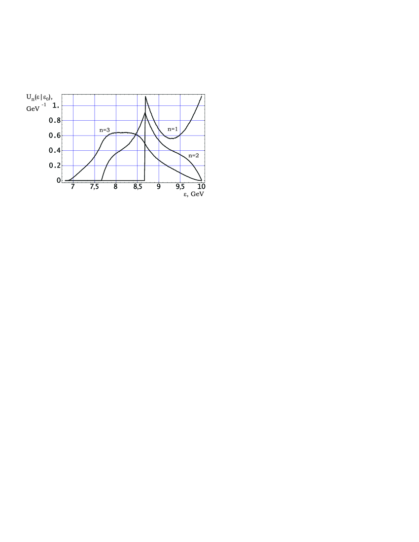
Figure 1: Energy spectra of electrons after $n$ = 1, 2, 3 collisions. $\varepsilon_{0}=10GeV,\,\omega_{0}=1eV.$

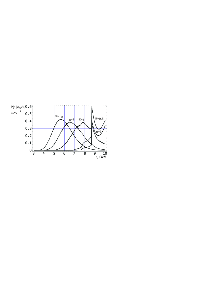
Figure 2: Energy spectra of electrons for $\overline{n}$ = 0.5, 1, 4, 7, 10. $\varepsilon_{0}=10GeV,\,\omega_{0}=1eV.$

It should be pointed out the discontinuous of the spectra for small $\overline{n}$ at the point $\varepsilon=\varepsilon_{0}-\omega_{\mathrm{max}}$ due to single scattered electrons and contribution of multiple scattered electrons at energies below the point of discontinuous. This contribution exists even for small $\overline{n}$.

It is seen from Fig. (2) that the width of the electron energy distributions decreases for such $\overline{n}$ which are greater than those one determined by Eq. (13).

The energy spectra of photons $\Phi(\omega|n)$ from the $n-$th scattering of electron and the resulting spectra for several $\overline{n}$ are shown in Fig. (3) and Fig. (4). It is seen from Fig. (4) that the contribution of multiple scattering should be taken into account even for the photon target of small thickness.

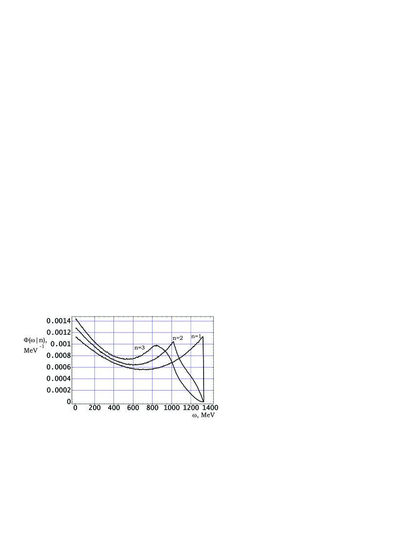
Figure 3: Energy spectra of photons generated in the $n$-th collision, $n$ = 1, 2, 3. $\varepsilon_{0}=10GeV,\,\omega_{0}=1eV.$

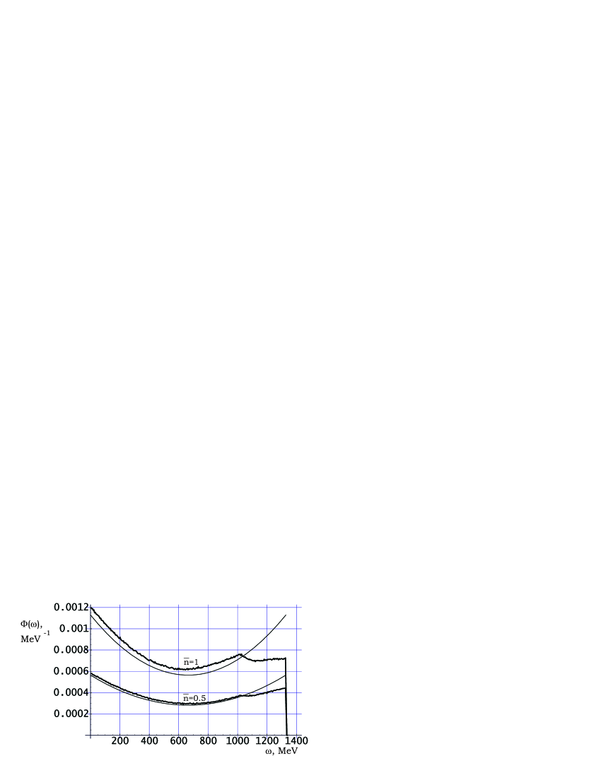
Figure 4: Energy spectra of photons for $\overline{n}$ = 0.5, 1. $\varepsilon_{0}=10GeV,\,\omega_{0}=1eV.$

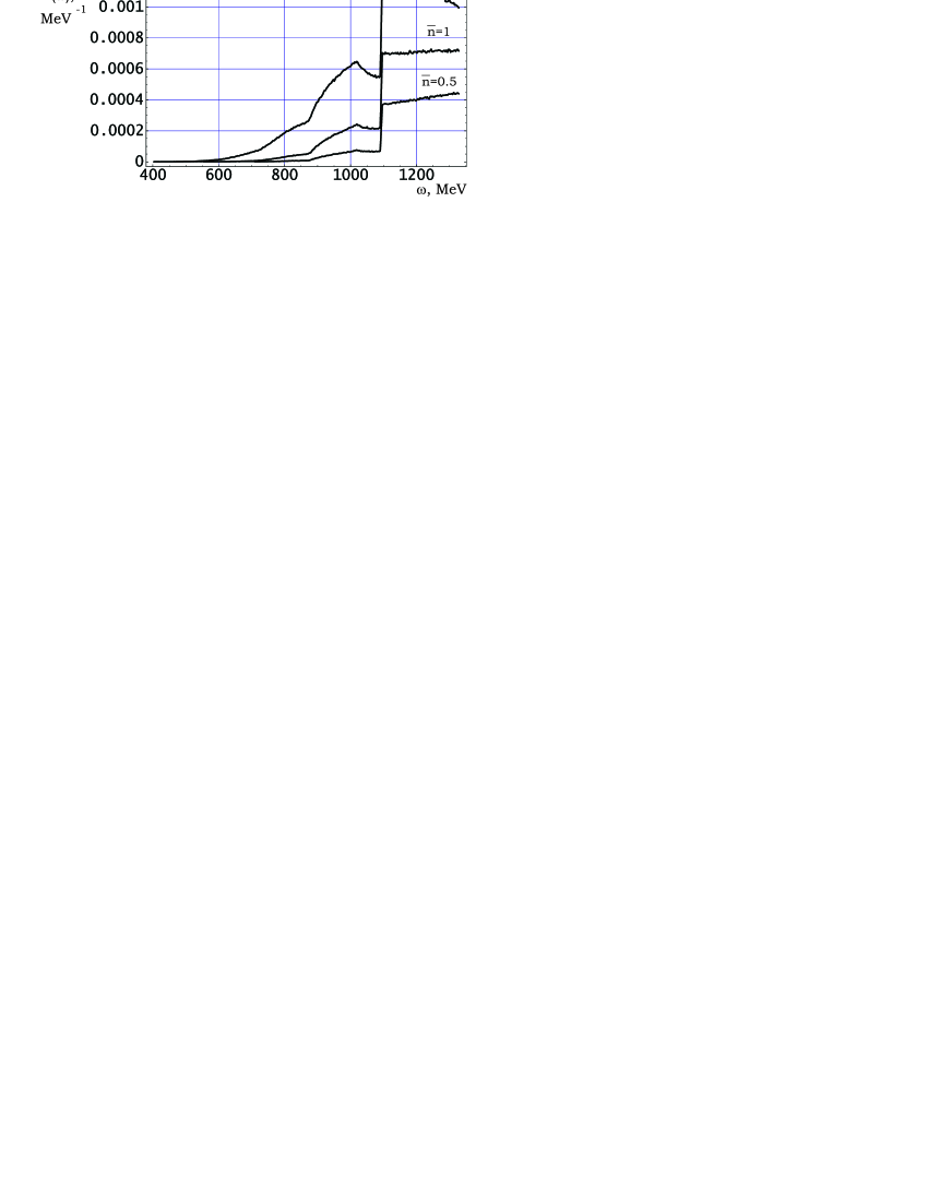
Figure 5: Energy spectra of photons with emission angle $\displaystyle\theta_{\mathrm{\gamma}}<\frac{1}{2}\,\frac{mc^{2}}{\varepsilon_{0}}$ for $\overline{n}$ = 0.5, 1, 2. $\varepsilon_{0}=10GeV,\,\omega_{0}=1eV.$

Fig. (5) shows that the electrons multiple collisions influence on the spectra of photons with emission angle $\displaystyle\theta_{\mathrm{\gamma}}<\frac{1}{2}\,\frac{mc^{2}}{\varepsilon_{0}}$. It is seen from the figure that multiple Compton scattering results in broadening of the photon spectra with increasing of the photon target thickness.

The mean energy loss of electrons in backward Compton scattering and the variance of the electron energy distribution are shown in Fig. (6) and Fig. (7).

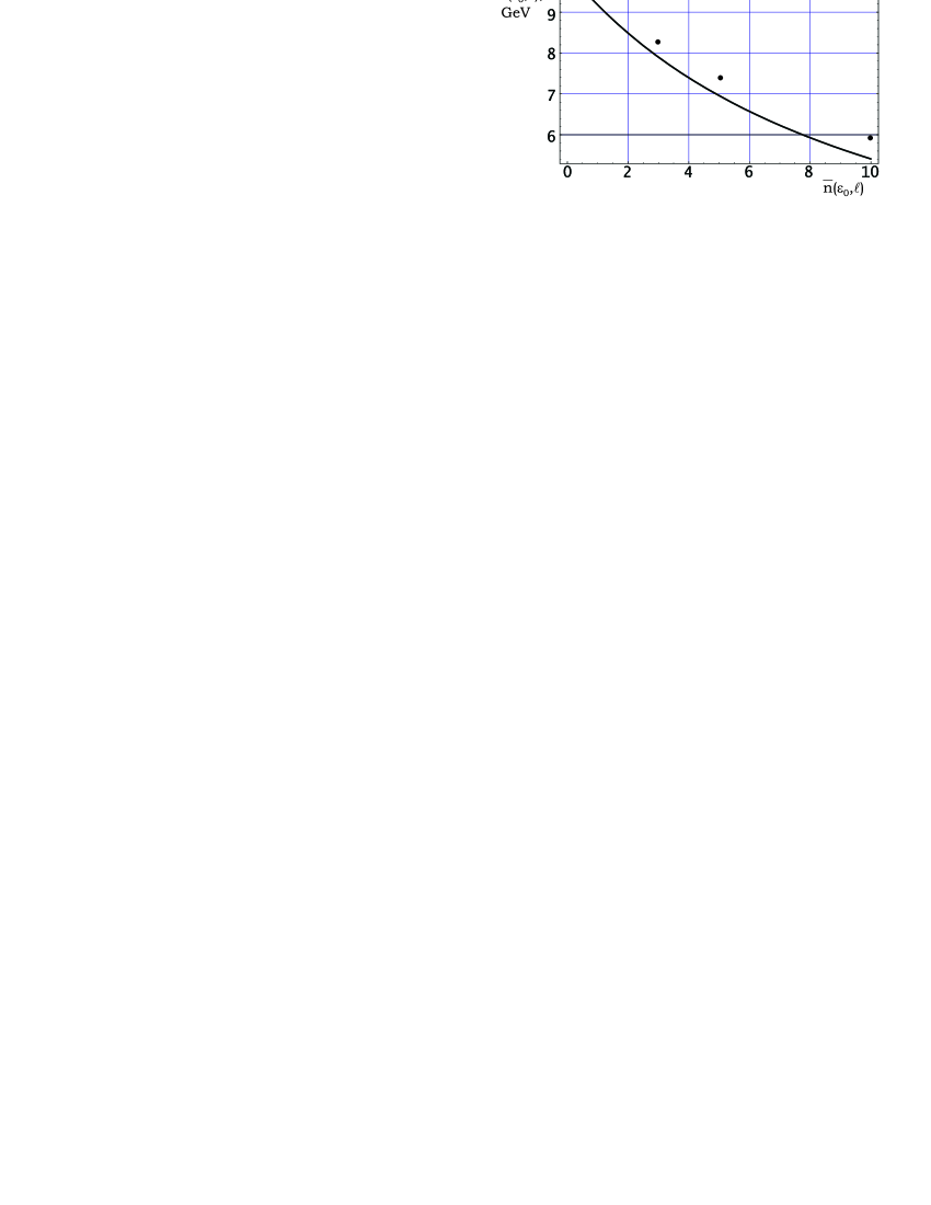
Figure 6: Mean energy of electron in back Compton scattering. $\varepsilon_{0}=10GeV,\,\omega_{0}=1eV.$ Points - simulation, solid line - Eq. (11).

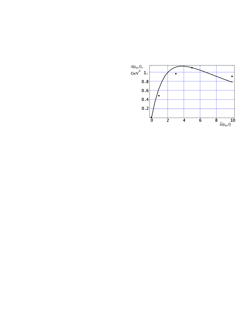
Figure 7: Variance of electron energy distribution. $\varepsilon_{0}=10GeV,\,\omega_{0}=1eV.$ Points - simulation, solid line - Eq. (12).

It is seen that the Monte Carlo data agree with the analytical calculations above.

References

[1]A.D.Angelo at al. Nucl. Instr. and Meth. 455 (2000), 1.
[2]I.Gizburg, G.Kotkin, V.Serbo, and V.Telnov. Nucl.Instr.
and Meth. 285 (1983) 47.
[3]V.Telnov. Nucl.Instr. and Meth. A 355 (1995) 3.
[4]V.Telnov. Nucl.Instr. and Meth. A 472 (2001) 43.
[5]W.Feller, An Introduction to Probability Theory and its
Application, Vols 1 and 2, Wiley, New York, 1971.
[6]A.M.Kolchuzhkin, V.V.Uchaikin, Introduction to the Theory of
Particles Penetration
through a Matter, (book in Russian). Moscow, Atomizdat, 1978.
[7]A.Kolchuzhkin, A.Potylitsyn, A.Bogdanov, I.Tropin, Physics Let.
A 264 (1999) 202.