VUTH 02-02 Estimate of the Collins fragmentation function in a chiral invariant approach

Abstract

We predict the features of the Collins function, which describes the fragmentation of a transversely polarized quark into an unpolarized hadron, by modeling the fragmentation into pions at a low energy scale. We use the chiral invariant approach of Manohar and Georgi, where constituent quarks and Goldstone bosons are considered as effective degrees of freedom in the non-perturbative regime of QCD. To test the approach we calculate the unpolarized fragmentation function and the transverse momentum distribution of a produced hadron, both of which are described reasonably well. In the case of semi-inclusive deep-inelastic scattering, our estimate of the Collins function in connection with the transversity distribution gives rise to a transverse single spin asymmetry of the order of 10%, supporting the idea of measuring the transversity distribution of the nucleon in this way. In the case of $e^{+}e^{-}$ annihilation into two hadrons, our model predicts a Collins azimuthal asymmetry of about 5%.

]

I Introduction

The influence of transverse spin and transverse momentum on fragmentation processes is at present a largely unexplored subject. The Collins fragmentation function [1], correlating the transverse spin of the fragmenting quark to the transverse momentum of the produced hadron, could give us the first chance to study this effect. Moreover, being chiral-odd, the Collins function can be connected to the transversity distribution function, which is chiral-odd as well, and thus can allow the measurement of this otherwise elusive property of the nucleon, which carries valuable information about the dynamics of confined quarks. Beside being chiral-odd, the Collins function is also time-reversal odd (T-odd).

In spite of the apparent difficulty in modeling T-odd effects, in a recent paper [2] we have shown that a non-vanishing Collins function can be obtained through a consistent one-loop calculation, in a description where massive constituent quarks and pions are the only effective degrees of freedom and interact via a simple pseudoscalar coupling.

In our previous work [2] little care has been devoted to the phenomenology of the Collins function. In contrast, our interest here lies in obtaining a reasonable estimate of this function and the observable effects induced by it. At present, only one attempt to theoretically estimate the Collins function for pions exists [3], and little phenomenological information is available from experiments. The HERMES collaboration reported the first measurements of single spin asymmetries in semi-inclusive DIS [4, 5], giving an indication of a possibly non-zero Collins function. The Collins function has also been invoked to explain large azimuthal asymmetries in $pp^{\uparrow}\rightarrow\pi X$ [6, 7]. In this case, however, the extraction of the function is plagued by large uncertainties, due to the possible presence of hadronic effects both in the initial and final state, and hence does not allow any conclusive statement yet. Recently, a phenomenological estimate of the Collins function has been proposed [8], combining results from the DELPHI, SMC and HERMES experiments. However, in spite of all the efforts to pin down the Collins function, the knowledge we have at present is still unsufficient.

In this work we calculate the Collins function for pions in a chiral invariant approach at a low energy scale. We use the model of Manohar and Georgi [9], which incorporates chiral symmetry and its spontaneous breaking, two important aspects of QCD at low energies. The spontaneous breaking of chiral symmetry leads to the existence of (almost massless) Goldstone bosons, which are included as effective degrees of freedom in the model. Quarks appear as further degrees of freedom as well. However, in contrast to the current quarks of the QCD Lagrangian, the model uses massive constituent quarks – a concept which has been proven very succesful in many phenomenological models at hadronic scales. With the exception of Ref. [10], the implications of a chiral invariant interaction for fragmentation functions into Goldstone bosons at low energy scales remains essentially unexplored. To investigate the Collins function for vector mesons like the $\rho$ [11] is beyond the reach of the approach.

Although the applicability of the Manohar-Georgi model is restricted to energies below the scale of chiral symmetry breaking $\Lambda_{\chi}\approx 1\,\rm{GeV}$, this is sufficient to calculate soft objects. In this kinematical regime, the chiral power counting allows setting up a consistent perturbation theory [12]. The relevant expansion parameter is given by $l/\Lambda_{\chi}$, where $l$ is a generic external momentum of a particle participating in the fragmentation. To guarantee the convergence of the perturbation theory, we restrict the maximum virtuality $\mu^{2}$ of the decaying quark to a soft value. We mostly consider the case $\mu^{2}=1\,\rm{GeV}^{2}$.

The outline of the paper is as follows: We first give the details of our model and present the analytical results of our calculation. Next, we discuss our results and compare them with known observables, indicating the choice of the parameters of our model. Then, we present the features of our prediction for the Collins function and its moments. Finally, using the outcome of our model, we estimate the leading order asymmetries containing the Collins function in semi-inclusive DIS and in $e^{+}e^{-}$ annihilation into two hadrons.

II Calculation of the Collins function

Considering the fragmentation process of a quark into a pion, $q^{\ast}(k)\to\pi(p)X$, we use the expressions of the unpolarized fragmentation function $D_{1}$ and the Collins function $H_{1}^{\perp}$ in terms of light-cone correlators, depending on the longitudinal momentum fraction $z$ of the pion and the transverse momentum $k_{{\scriptscriptstyle T}}$ of the quark. The definitions read [13, 14]

$$D_{1}(z,z^{2}k^{2}_{{\scriptscriptstyle T}})=\left.\frac{1}{4z}\int{\rm\,d}k^{+}\;\mbox{Tr}\,[\Delta(k,p)\gamma^{-}]\right|_{k^{-}=\frac{p^{-}}{z}}\,,$$ (1)

$$\frac{\epsilon_{{\scriptscriptstyle T}}^{ij}k_{{\scriptscriptstyle T}\,j}}{m_{\pi}}\,H_{1}^{\perp}(z,z^{2}k^{2}_{{\scriptscriptstyle T}})$$ (2)

$$\quad\quad\quad\quad\mbox{}=\left.\frac{1}{4z}\int{\rm\,d}k^{+}\;\mbox{Tr}\,[\Delta(k,p){\rm i}\sigma^{i-}\gamma_{5}]\right|_{k^{-}=\frac{p^{-}}{z}}\,,$$ (3)

with $m_{\pi}$ denoting the pion mass and $\epsilon_{{\scriptscriptstyle T}}^{ij}\equiv\epsilon^{ij-+}$ (we specify the plus and minus lightcone components of a generic 4-vector $a^{\mu}$ according to $a^{\pm}\equiv(a^{0}\pm a^{3})/\sqrt{2}$). The correlation function $\Delta(k,p)$ in Eqs. (1, 3), omitting gauge links, takes the form

$$\Delta(k,p)=\sum_{X}\,\int \frac{{\rm\,d}^{4}\xi}{(2\pi)^{4}}\;{\rm e}^{+{\rm i}k\cdot\xi}\langle 0|\,\psi(\xi)|\pi,X\rangle$$ (5)

$$\mbox{}\times\langle\pi,X|\bar{\psi}(0)|0\rangle\,.$$

We now use the chiral invariant model of Manohar and Georgi [9] to calculate the matrix elements in the correlation function. Neglecting the part that describes free Goldstone bosons, the Lagrangian of the model reads

$${\cal L}=\bar{\psi}\,({\rm i}\hbox to0.0pt{/\hss}\partial+\hbox to0.0pt{/\hss}V-m+g_{{\scriptscriptstyle A}}\hbox to0.0pt{/\hss}A\gamma_{5})\,\psi\,.$$ (6)

In Eq. (6) the pion field enters through the vector and axial vector combinations

$$V^{\mu}=\frac{{\rm i}}{2}\,[u^{\dagger},\partial^{\mu}u]\,,\qquad A^{\mu}=\frac{{\rm i}}{2}\,\{u^{\dagger},\partial^{\mu}u\}\,,$$ (7)

with $u=\textrm{exp}({\rm i}\,\vec{\tau}\!\cdot\!\vec{\pi}/2F_{\pi})$, where the $\tau_{i}$ are the generators of the SU(2) flavour group and $F_{\pi}=93\,\textrm{MeV}$ represents the pion decay constant. In absence of resonances, the pion decay constant determines the scale of chiral symmetry breaking via $\Lambda_{\chi}=4\pi F_{\pi}$. The quark mass $m$ and the axial coupling constant $g_{{\scriptscriptstyle A}}$ are free parameters of the model that are not constrained by chiral symmetry. The values of these parameters will be specified in Sec. III. Though we limit ourselves here to the SU(2) flavour sector of the model, the extension to strange quarks is straightforward, allowing in particular the calculation of kaon fragmentation functions. For convenience we write down explicitly those terms of the interaction part of the Lagrangian (6) that are relevant for our calculation. To be specific we need both the interaction of a single pion with a quark and the two-pion contact interaction, which can be easily obtained by expanding the non-linear representation $u$ in terms of the pion field:

$${\cal L}_{\pi qq} = -\frac{g_{\scriptscriptstyle A}}{2F_{\pi}}\bar{\psi}\gamma_{\mu}\gamma_{5}\vec{\tau}\cdot\partial^{\mu}\vec{\pi}\psi\,,$$ (8)

$${\cal L}_{\pi\pi qq} = -\frac{1}{4F_{\pi}^{2}}\bar{\psi}\gamma_{\mu}\vec{\tau}\cdot(\vec{\pi}\times\partial^{\mu}\vec{\pi})\psi\,.$$ (9)

Performing the numerical calculation of the Collins function, it turns out that the contact interaction (9), which is a direct consequence of chiral symmetry, plays a dominant role.

At tree level, the fragmentation of a quark is modeled through the process $q^{\ast}\to\pi q$, where Fig. 1 represents the corresponding unitarity diagram. Using the Lagrangian in Eq. (8), the correlation function at lowest order reads

$$\Delta_{(0)}(k,p) = -\frac{g_{\scriptscriptstyle A}^{2}}{4F_{\pi}^{2}}\frac{1}{(2\pi)^{4}}\,\frac{(\hbox to0.0pt{/\hss}k+m)}{k^{2}-m^{2}}\,\gamma_{5}\,\hbox to0.0pt{/\hss}p\,(\hbox to0.0pt{/\hss}k-\hbox to0.0pt{/\hss}p+m)$$ (11)

$$\mbox{}\times\hbox to0.0pt{/\hss}p\,\gamma_{5}\frac{(\hbox to0.0pt{/\hss}k+m)}{k^{2}-m^{2}}\,2\pi\,\delta((k-p)^{2}-m^{2})\,.$$

This correlation function allows to compute the unpolarized fragmentation function $D_{1}$ by means of Eq. (1), leading to

$$D_{1}(z,z^{2}k^{2}_{\scriptscriptstyle T}) = \frac{1}{z}\frac{g_{\scriptscriptstyle A}^{2}}{4F_{\pi}^{2}}\frac{1}{16\pi^{3}}$$ (13)

$$\mbox{}\times\bigg{(}1-4\frac{1-z}{z^{2}}\frac{m^{2}m_{\pi}^{2}}{[k_{\scriptscriptstyle T}^{2}+m^{2}+\frac{1-z}{z^{2}}m_{\pi}^{2}]^{2}}\bigg{)}.$$

Note that the expression in (13) is only weakly dependent on the transverse momentum of the quark. In fact, $D_{1}$ is constant as a function of $k_{\scriptscriptstyle T}$, if $m_{\pi}=0$ and (or) $m=0$. Because our approach is limited to a soft regime, we will impose an upper cutoff on the $k_{\scriptscriptstyle T}$ integration, as will be discussed in more detail in Sec. III. This in turn leads to a finite $D_{1}(z)$ after integration over the transverse momentum.

The SU(2) flavour structure of our approach implies the relations

$$D_{1}^{u\rightarrow\pi^{0}}=D_{1}^{\bar{u}\rightarrow\pi^{0}}=D_{1}^{d\rightarrow\pi^{0}}=D_{1}^{\bar{d}\rightarrow\pi^{0}} = D_{1}\,,$$ (14)

$$D_{1}^{u\rightarrow\pi^{+}}=D_{1}^{\bar{d}\rightarrow\pi^{+}}=D_{1}^{\bar{u}\rightarrow\pi^{-}}=D_{1}^{d\rightarrow\pi^{-}} = 2\,D_{1}\,,$$ (15)

where $D_{1}$ is the result given in Eq. (13). In the case of unfavoured fragmentation processes $D_{1}$ vanishes at tree level, but will be non-zero as soon as one-loop corrections are included. According to the chiral power counting, one-loop contributions to $D_{1}$ are suppressed by a factor $l^{2}/\Lambda_{\chi}^{2}$ compared to the tree level result. The maximum momentum up to which the chiral perturbation expansion converges numerically can only be determined by an explicit calculation of the one-loop corrections.

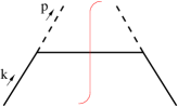
FIG. 1.: Lowest-order unitarity diagram describing the fragmentation of a quark into a pion.

Like in the case of a pseudoscalar quark-pion coupling [2], the Collins function $H_{1}^{\perp}$ turns out to be zero in Born approximation. To obtain a non-zero result, we have to resort to the one-loop level. In Fig. 2 the corresponding diagrams are shown, where we have displayed only those graphs that contribute to the Collins function. The explicit calculation of $H_{1}^{\perp}$ is similar to our previous work [2]. The relevant ingredients of the calculation are the self-energy and the vertex correction diagrams. These ingredients are sketched in Fig. 3 and can be expressed analytically as

$$-{\rm i}\Sigma(k)=\frac{g_{\scriptscriptstyle A}^{2}}{4F_{\pi}^{2}}\int\frac{{\rm\,d}^{4}l}{(2\pi)^{4}}\,\frac{\hbox to0.0pt{/\hss}l\,(\hbox to0.0pt{/\hss}k-\hbox to0.0pt{/\hss}l-m)\,\hbox to0.0pt{/\hss}l}{[(k-l)^{2}-m^{2}]\,[l^{2}-m_{\pi}^{2}]}\,,$$ (16)

$$\Gamma_{1}(k,p)=-{\rm i}\frac{g_{\scriptscriptstyle A}^{3}}{8F_{\pi}^{3}}\gamma_{5}\int\frac{{\rm\,d}^{4}l}{(2\pi)^{4}}$$ (17)

$$\quad\mbox{}\times\frac{\hbox to0.0pt{/\hss}l\,(\hbox to0.0pt{/\hss}k-\hbox to0.0pt{/\hss}p-\hbox to0.0pt{/\hss}l+m)}{[(k-p-l)^{2}-m^{2}]}\frac{\hbox to0.0pt{/\hss}p\,(\hbox to0.0pt{/\hss}k-\hbox to0.0pt{/\hss}l-m)\,\hbox to0.0pt{/\hss}l}{[(k-l)^{2}-m^{2}][l^{2}-m_{\pi}^{2}]}\,,$$ (18)

$$\Gamma_{2}(k,p)=-{\rm i}\frac{g_{\scriptscriptstyle A}}{8F_{\pi}^{3}}\gamma_{5}\int\frac{{\rm\,d}^{4}l}{(2\pi)^{4}}$$ (19)

$$\quad\mbox{}\times\frac{(\hbox to0.0pt{/\hss}l+\hbox to0.0pt{/\hss}p)\,(\hbox to0.0pt{/\hss}l-\hbox to0.0pt{/\hss}k+m)\,\hbox to0.0pt{/\hss}l}{[(k-l)^{2}-m^{2})][l^{2}-m_{\pi}^{2}]}\,,$$ (20)

where flavour factors have been suppressed. For later purpose, we give here the most general parametrization of the functions $\Sigma$, $\Gamma_{1}$ and $\Gamma_{2}$,

$$\Sigma(k) = A\,\hbox to0.0pt{/\hss}k+B\,m\,,\vphantom{\frac{1}{1}}$$ (21)

$$\Gamma_{1}(k,p) = \frac{g_{\scriptscriptstyle A}}{2F_{\pi}}\gamma_{5}\Big{(}C_{1}+D_{1}\,\hbox to0.0pt{/\hss}p+E_{1}\,\hbox to0.0pt{/\hss}k+F_{1}\,\hbox to0.0pt{/\hss}p\,\hbox to0.0pt{/\hss}k\Big{)}\,,$$ (22)

$$\Gamma_{2}(k,p) = \frac{g_{\scriptscriptstyle A}}{2F_{\pi}}\gamma_{5}\Big{(}C_{2}+D_{2}\,\hbox to0.0pt{/\hss}p+E_{2}\,\hbox to0.0pt{/\hss}k+F_{2}\,\hbox to0.0pt{/\hss}p\,\hbox to0.0pt{/\hss}k\Big{)}\,.$$ (23)

The real parts of the functions $A$, $B$, $C_{1}$, $D_{1}$ etc. could be UV-divergent and require in principle a proper renormalization. Here, we don’t need to deal with the question of renormalization at all, since only the imaginary parts of the loop diagrams are important when calculating the Collins function [2].

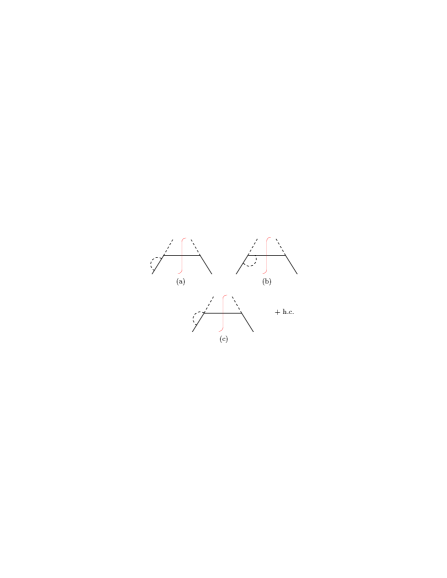
FIG. 2.: One-loop corrections to the fragmentation of a quark into a pion contributing to the Collins function. The hermitian conjugate diagrams (h.c.) are not shown explicitly.

FIG. 3.: One-loop self-energy, and vertex corrections.

Taking now flavour factors properly into account, the contributions to the correlation function generated by the diagrams (a), (b) and (c) in Fig. 2 are given by

$$\Delta_{(1)}^{(a)}(k,p)=-3\frac{g_{\scriptscriptstyle A}^{2}}{4F_{\pi}^{2}}\frac{1}{(2\pi)^{4}}\,\frac{(\hbox to0.0pt{/\hss}k+m)}{k^{2}-m^{2}}\,\gamma_{5}\,\hbox to0.0pt{/\hss}p\,(\hbox to0.0pt{/\hss}k-\hbox to0.0pt{/\hss}p+m)\,$$ (24)

$$\qquad\mbox{}\times\hbox to0.0pt{/\hss}p\,\gamma_{5}\frac{(\hbox to0.0pt{/\hss}k+m)}{k^{2}-m^{2}}\,\Sigma(k)\,\frac{(\hbox to0.0pt{/\hss}k+m)}{k^{2}-m^{2}}\,$$ (25)

$$\qquad\mbox{}\times 2\pi\,\delta((k-p)^{2}-m^{2})\,,\vphantom{\frac{1}{1}}$$ (26)

$$\Delta_{(1)}^{(b)}(k,p)=\frac{g_{\scriptscriptstyle A}}{2F_{\pi}^{2}}\frac{1}{(2\pi)^{4}}\,\frac{(\hbox to0.0pt{/\hss}k+m)}{k^{2}-m^{2}}\,\gamma_{5}\,\hbox to0.0pt{/\hss}p\,(\hbox to0.0pt{/\hss}k-\hbox to0.0pt{/\hss}p+m)$$ (27)

$$\qquad\mbox{}\times\Gamma_{1}(k,p)\frac{(\hbox to0.0pt{/\hss}k+m)}{k^{2}-m^{2}}\,2\pi\,\delta((k-p)^{2}-m^{2})\,,$$ (28)

$$\Delta_{(1)}^{(c)}(k,p)=-2\frac{g_{\scriptscriptstyle A}}{2F_{\pi}^{2}}\frac{1}{(2\pi)^{4}}\,\frac{(\hbox to0.0pt{/\hss}k+m)}{k^{2}-m^{2}}\,\gamma_{5}\,\hbox to0.0pt{/\hss}p\,(\hbox to0.0pt{/\hss}k-\hbox to0.0pt{/\hss}p+m)$$ (29)

$$\qquad\mbox{}\times\Gamma_{2}(k,p)\frac{(\hbox to0.0pt{/\hss}k+m)}{k^{2}-m^{2}}\,2\pi\,\delta((k-p)^{2}-m^{2})\,.$$ (30)

The correlation functions of the hermitian conjugate diagrams follow from the hermiticity condition $\Delta_{(1)}^{h.c.}(k,p)=\gamma^{0}\Delta_{(1)}^{\dagger}(k,p)\gamma^{0}$.

Summing the contributions of all diagrams and inserting the resulting correlation function in Eq. (3), we eventually obtain the result

$$H_{1}^{\perp}(z,z^{2}k^{2}_{{\scriptscriptstyle T}})=\frac{g_{\scriptscriptstyle A}^{2}}{32\pi^{3}F_{\pi}^{2}}\frac{m_{\pi}}{1-z}\frac{1}{k^{2}-m^{2}}$$ (31)

$$\quad\mbox{}\times\bigg{(}-3m\,{\rm Im}\,\big{(}A+B\big{)}$$ (32)

$$\quad-\,{\rm Im}\,\big{(}C_{1}\!-mE_{1}+(k^{2}\!-m^{2})F_{1}\big{)}\vphantom{\frac{1}{1}}$$ (33)

$$\quad+2\,{\rm Im}\,\big{(}C_{2}\!-mE_{2}+(k^{2}\!-m^{2})F_{2}\big{)}\!\bigg{)}\!\bigg{|}_{k^{2}=\frac{z}{1-z}k_{{\scriptscriptstyle T}}^{2}+\frac{m^{2}}{1-z}+\frac{m_{\pi}^{2}}{z}}\,.$$ (34)

Thus, the Collins function is entirely given by the imaginary parts of the coefficients defined in Eqs. (21–23). We can compute these imaginary parts by applying Cutkosky rules to the self-energy and vertex diagrams of Fig. 3. Explicit calculation leads to

$$\,{\rm Im}\,\big{(}A+B\big{)}=\frac{g_{\scriptscriptstyle A}^{2}}{32\pi^{2}F_{\pi}^{2}}$$ (35)

$$\quad\mbox{}\times\bigg{(}2m_{\pi}^{2}-\frac{k^{2}-m^{2}}{2}\Big{(}1-\frac{m^{2}-m_{\pi}^{2}}{k^{2}}\Big{)}\bigg{)}I_{1}\,,$$ (36)

$$\,{\rm Im}\,\big{(}C_{1}-mE_{1}+(k^{2}-m^{2})F_{1}\big{)}=\frac{g_{\scriptscriptstyle A}^{2}}{32\pi^{2}F_{\pi}^{2}}$$ (37)

$$\quad\mbox{}\times m\,(k^{2}-m^{2})\bigg{(}\frac{3k^{2}+m^{2}-m_{\pi}^{2}}{2k^{2}}I_{1}$$ (38)

$$\quad\mbox{}+4m^{2}\frac{k^{2}-m^{2}+m_{\pi}^{2}}{\lambda(k^{2},m^{2},m_{\pi}^{2})}\Big{(}I_{1}+(k^{2}-m^{2}-2m_{\pi}^{2})I_{2}\Big{)}\bigg{)}\,,$$ (39)

$$\,{\rm Im}\,\big{(}C_{2}-mE_{2}+(k^{2}-m^{2})F_{2}\big{)}=\frac{1}{32\pi^{2}F_{\pi}^{2}}$$ (40)

$$\quad\mbox{}\times m\,(k^{2}-m^{2})\bigg{(}1-\frac{m^{2}-m_{\pi}^{2}}{k^{2}}\bigg{)}I_{1}\,,$$ (41)

where we have introduced the so-called Källen function, $\lambda(k^{2},m^{2},m_{\pi}^{2})=[k^{2}-(m+m_{\pi})^{2}][k^{2}-(m-m_{\pi})^{2}]$, and the factors

$$I_{1} = \int{\rm\,d}^{4}l\;\delta(l^{2}-m_{\pi}^{2})\,\delta((k-l)^{2}-m^{2})$$ (42)

$$= \frac{\pi}{2k^{2}}\sqrt{\lambda(k^{2},m^{2},m_{\pi}^{2})}\;\theta(k^{2}-(m+m_{\pi})^{2})\,,$$ (43)

$$I_{2} = \int{\rm\,d}^{4}l\;\frac{\delta(l^{2}-m_{\pi}^{2})\,\delta((k-l)^{2}-m^{2})}{(k-p-l)^{2}-m^{2}}$$ (44)

$$= -\frac{\pi}{2\sqrt{\lambda(k^{2},m^{2},m_{\pi}^{2})}}\ln{\left|1+\frac{\lambda(k^{2},m^{2},m_{\pi}^{2})}{k^{2}m^{2}-(m^{2}-m_{\pi}^{2})^{2}}\right|}$$ (46)

$$\mbox{}\times\theta(k^{2}-(m+m_{\pi})^{2})\,.\vphantom{\frac{1}{1}}$$

These integrals are finite and vanish below the threshold of quark-pion production, where the self-energy and vertex diagrams do not possess an imaginary part.

Thus, Eq. (33) in combination with Eqs. (36)–(46) gives the explicit result for the Collins function in the Manohar-Georgi model to lowest possible order. Because of its chiral-odd nature, the Collins function would vanish in this model if we set the mass of the quark to zero. The same phenomenon has been observed in the calculation of a chiral-odd twist-3 fragmentation function [10]. The result in Eq. (33) corresponds, e.g., to the fragmentation $u\to\pi^{0}$. The expressions of the remaining favoured transitions are obtained in analogy to Eqs. (14,15). Unfavoured fragmentation processes in the case of the Collins function appear only at the two-loop level.

III Estimates and phenomenology

A Unpolarized fragmentation function and the choice of parameters

We now present our numerical estimates, where all results for the fragmentation functions in this subsection refer to the transition $u\to\pi^{+}$. To begin with we calculate the unpolarized fragmentation function $D_{1}(z)$ which is given by

$$D_{1}(z)=\pi\int_{0}^{K^{2}_{{\scriptscriptstyle T}\,{\rm max}}}{\rm\,d}K^{2}_{{\scriptscriptstyle T}}\;D_{1}(z,K^{2}_{{\scriptscriptstyle T}}),$$ (47)

where $\vec{K}_{{\scriptscriptstyle T}}=-z\vec{k}_{{\scriptscriptstyle T}}$ denotes the transverse momentum of the outgoing hadron with respect to the quark direction. The upper limit on the $K^{2}_{{\scriptscriptstyle T}}$ integration is set by the cutoff on the fragmenting quark virtuality, $\mu^{2}$, and corresponds to

$$K^{2}_{{\scriptscriptstyle T}\,{\rm max}}=z\,(1-z)\,\mu^{2}-z\,m^{2}-(1-z)\,m_{\pi}^{2}\,.$$ (48)

Besides $m$ and $g_{\scriptscriptstyle A}$, the cutoff $\mu^{2}$ is the third parameter of our approach that is not fixed a priori. However, as will be explained below, the possible values of $\mu^{2}$ can be restricted when comparing our results to experimental data. Unless otherwise specified, we always use the values

$$m=0.3\;{\rm GeV},\qquad g_{{\scriptscriptstyle A}}=1,\qquad\mu^{2}=1\;{\rm GeV}^{2}\,.$$ (49)

At the relevant places, the dependence of our results on possible variations of these parameters will be discussed. Few remarks concerning the choice in (49) are in order. The value of $m$ is a typical mass of a constituent quark. The choice for the axial coupling can be seen as a kind of average number of what has been proposed in the literature. For instance, in a simple SU(6) spin-flavour model for the proton one finds $g_{\scriptscriptstyle A}\approx 0.75$ in order to obtain the correct value for the axial charge of the nucleon [9]. On the other side, large $N_{c}$ arguments favour a value of the order of one [15], while, according to a recent calculation in a relativistic point-form approach [16], a $g_{\scriptscriptstyle A}$ slightly above one seems to be required for describing the axial charge of the nucleon. Finally, our choice for $\mu^{2}$ ensures that the momenta of the outgoing pion and quark, in the rest-frame of the fragmenting quark, remain below values of the order $0.5\,\rm{GeV}$. In this region we believe chiral perturbation theory to be applicable, meaning that our leading order result should provide a reliable estimate.

In Fig. 4 we show the result for the unpolarized fragmentation function $D_{1}^{u\rightarrow\pi^{+}}$. Notice that in general the fragmentation functions vanish outside the kinematical limits, which in our model are given by

$$z_{{\rm max},{\rm min}} = \frac{1}{2}\Biggl{[}\left(1-\frac{m^{2}-m_{\pi}^{2}}{\mu^{2}}\right)$$ (51)

$$\qquad\pm\sqrt{\left(1-\frac{m^{2}-m_{\pi}^{2}}{\mu^{2}}\right)^{2}-4\,\frac{m_{\pi}^{2}}{\mu^{2}}}\Biggr{]},$$

corresponding to the situation when the upper limit of the $K_{{\scriptscriptstyle T}}^{2}$ integration becomes equal to zero. We consider our tree level result as a pure valence-type part of $D_{1}^{u\rightarrow\pi^{+}}$. The sea-type (unfavoured) transition $\bar{u}\to\pi^{+}$ is strictly zero at leading order. Therefore, we compare the model result to the valence-type quantity $D_{1}^{u\rightarrow\pi^{+}}-D_{1}^{\bar{u}\rightarrow\pi^{+}}$, where the fragmentation functions have been taken from the parametrization of Kretzer [17] at a scale $Q^{2}=1\,\rm{GeV}^{2}$. Obviously, the $z$-dependence of both curves is in nice agreement. We point out that such an agreement is non-trivial. For example, in the pseudoscalar model that we used in our previous work [2], $D_{1}$ behaves quite differently and peaks at an intermediate $z$-value.

On the other side, we underestimate the parametrization of Ref. [17] by about a factor of two. Some remarks are in order at this point. Although a part of the discrepancy might be attributed to the uncertainty in the value of $g_{\scriptscriptstyle A}$, the most important point is to address the question as to what extent we can compare our estimate with existing parametrizations. The parametrization of [17] serves basically as input function of the pQCD evolution equations, used to describe high-energy $e^{+}e^{-}$ data, and displays the typical logarithmic dependence on the scale $Q^{2}$. A value of $Q^{2}=1$ GeV² is believed to be already beyond the limit of applicability of pQCD calculations. On the other side, our approach displays, to a first approximation, a linear dependence on the cutoff $\mu^{2}$. It is supposed to be valid at low scales and it is also stretched to the limit of its applicability for $\mu^{2}=1$ GeV². In this context it should also be investigated to what extent the inclusion of one-loop corrections, which allow for the additional decay channel $q^{\ast}\to\pi\pi q$, will increase the result for $D_{1}$ at $\mu^{2}=1\,\rm{GeV}^{2}$. Finally, we want to remark that to our knowledge there exists no strict one-to-one correspondence between the quark virtuality $\mu^{2}$ and the scale used in the evolution equation of fragmentation functions, which in semi-inclusive DIS, e.g., is typically identified with the photon virtuality $Q^{2}$. For all these reasons, a smooth matching of our calculation and the parametrization of [17] cannot necessarily be expected. Despite these caveats, the correct $z$-behaviour displayed by our result for $D_{1}$ suggests that the calculation can well be used as an input for evolution equations at a low scale. In the next subsection we will elaborate more on this point in connection with the Collins function.

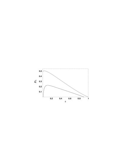
FIG. 4.: Model result for the unpolarized quark fragmentation function $D_{1}^{u\rightarrow\pi^{+}}$ (solid line) and comparison with a parametrization of Ref. [17] (grey line).

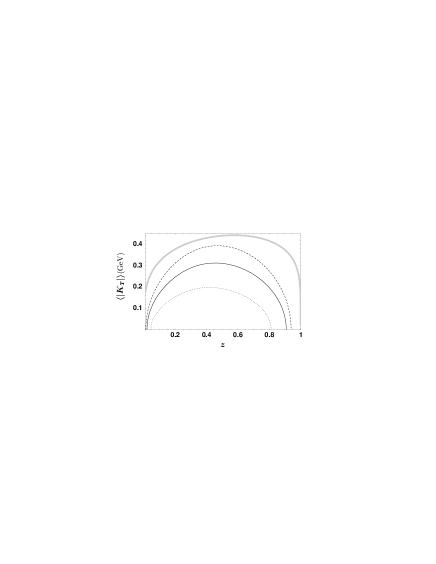
FIG. 5.: Model result for the average hadron transverse momentum for different choices of the cutoff: $\mu^{2}=0.5$ GeV² (dotted line), $\mu^{2}=1$ GeV² (solid line), $\mu^{2}=1.5$ GeV² (dashed line) and comparison with a fit to experimental results from DELPHI [21] (grey line).

The best indication of the appropriate value of the cutoff $\mu^{2}$ may be obtained when comparing our calculation to experimental data of the average transverse momentum of the outgoing hadron with respect to the quark, which we evaluate according to

$$\langle|\vec{K}_{{\scriptscriptstyle T}}|\rangle(z)=\frac{\pi}{D_{1}(z)}\int_{0}^{K^{2}_{{\scriptscriptstyle T}\,{\rm max}}}{\rm\,d}K^{2}_{{\scriptscriptstyle T}}\,|\vec{K}_{{\scriptscriptstyle T}}|\,D_{1}(z,K^{2}_{{\scriptscriptstyle T}})\,.$$ (52)

In Fig. 5 we show the result of this observable as a function of $z$ for three different choices of the parameter $\mu^{2}$. As a comparison, we also show a fit (taken from Ref. [6]) to experimental data obtained by the DELPHI collaboration [21]. Like in the case of $D_{1}(z)$, the shape of our result is very similar to the experimental one, which we consider as an encouraging result. For $\mu^{2}=1\,\rm{GeV}^{2}$ our curve is about $30\%$ below the data. Such a disagreement is not surprising, keeping in mind that at LEP energies higher order pQCD effects (e.g. gluon bremsstrahlung, unfavoured fragmentations, etc.) play an important role, leading in general to a broadening of the $K_{\scriptscriptstyle T}$ distribution. For experiments at lower energies, however, where pQCD contributions can be neglected in a first approximation, it may be possible to exhaust the experimental value for $\langle|\vec{K}_{{\scriptscriptstyle T}}|\rangle(z)$ with genuine soft contributions as described in our model. This in turn would determine the appropriate value of the cutoff $\mu^{2}$. For example, such a method of matching our calculation with experimental conditions could be applied at HERMES kinematics, even though the method is somewhat hampered since $K_{\scriptscriptstyle T}$ is not directly measured in semi-inclusive DIS. In this case, one rather observes the transverse momentum of the outgoing hadron with respect to the virtual photon, $P_{h\perp}$, which depends on both $K_{\scriptscriptstyle T}$ and the transverse momentum of the partons inside the target $p_{\scriptscriptstyle T}$. At leading order in the hard scattering cross section one can in fact derive the relation

$$\langle P^{2}_{h\perp}\rangle(x,z)$$ (53)

$$\qquad= z^{2}\frac{\pi\int{\rm\,d}p^{2}_{{\scriptscriptstyle T}}\,p_{{\scriptscriptstyle T}}^{2}\,f_{1}(x,p^{2}_{{\scriptscriptstyle T}})}{f_{1}(x)}+\frac{\pi\int{\rm\,d}K^{2}_{{\scriptscriptstyle T}}\,K_{{\scriptscriptstyle T}}^{2}\,D_{1}(z,K^{2}_{{\scriptscriptstyle T}})}{D_{1}(z)}$$ (54)

$$\qquad= z^{2}\,\langle p^{2}_{{\scriptscriptstyle T}}\rangle(x)+\langle K^{2}_{{\scriptscriptstyle T}}\rangle(z)\,,$$ (55)

where $x$ represents the Bjorken variable.

B Collins function

We now turn to the description of our model result for the Collins function. In Fig. 6, $H_{1}^{\perp}$ is plotted for three different values of the constituent quark mass, $m=0.2,\,0.3,\,0.4$ GeV. In a large $z$-range, the function does not depend strongly on the precise value of the quark mass, if we choose it within reasonable limits. That’s why we can confidently fix $m=0.3\,\rm{GeV}$ for our numerical studies. It is very interesting to observe that the behaviour of the unpolarized fragmentation function $D_{1}$ is quite distinct from that of the Collins function: while the former is decreasing as $z$ increases, the latter is growing.

FIG. 6.: Model result for the Collins function for different values of the constituent quark mass: $m=0.2$ GeV (dotted line), $m=0.3$ GeV (solid line), $m=0.4$ GeV (dashed line).

The different behaviour of the two functions becomes even more evident when looking at their ratio, shown in Fig. 7. We emphasize that also from the experimental side there exists some evidence for an increasing ratio $H_{1}^{\perp}/D_{1}$. In a recent analysis of the longitudinal single spin asymmetry measured at HERMES, Efremov et al. [8] extracted a behaviour $H_{1}^{\perp}/D_{1}\propto z$ for $z\leq 0.7$. We consider the agreement in finding a clearly rising ratio $H_{1}^{\perp}/D_{1}$ as remarkable, even though in the analysis of Ref. [8] some simplifying assumptions have been used in order to obtain information on $H_{1}^{\perp}$ from data taken with a longitudinally polarized target. It will be very interesting to see if dedicated future experiments can confirm such a behaviour. We also mention that ratios of the Collins function or any of its moments with $D_{1}$ are almost independent of the coupling constant $g_{{\scriptscriptstyle A}}$. The reason is that the one-loop correction containing the contact interaction is only proportional to $g_{{\scriptscriptstyle A}}^{2}$, as $D_{1}$ is, and is dominating on the others. Furthermore, the ratio $H_{1}^{\perp}/D_{1}$ is nearly independent of the cutoff $\mu^{2}$. In conclusion, the prediction shown in Fig. 7 is almost independent of the choice of parameters in our approach.

FIG. 7.: Model result for $H_{1}^{\perp}/D_{1}$.

At this point we would like to add some general remarks concerning the $z$-behaviour of our results. It turns out that the shape of all the results does not vary much when changing the parameters within reasonable limits. In particular, variations of $g_{\scriptscriptstyle A}$ and of the cutoff $\mu^{2}$ only change the normalization of the curves but not their shape. In this sense our calculation of fragmentation functions has a strong predictive power. This has a direct practical consequence if one uses, for instance, our result of the Collins function as input in an evolution equation: the $z$-dependence of the input function can be adjusted to the shape of our $H_{1}^{\perp}$, while its normalization can be kept free in order to account for uncertainties in the values of $g_{\scriptscriptstyle A}$ and $\mu^{2}$.

In Fig. 8 we plot the ratio

$$\frac{H_{1}^{\perp(\frac{1}{2})}(z)}{D_{1}(z)}\equiv\frac{\pi}{D_{1}(z)}\int{\rm\,d}K_{{\scriptscriptstyle T}}^{2}\,\frac{|\vec{K}_{{\scriptscriptstyle T}}|}{2zm_{\pi}}\,H_{1}^{\perp}(z,K_{{\scriptscriptstyle T}}^{2})\,,$$ (56)

which enters the transverse single spin asymmetry to be discussed in the following subsection. This quantity rises roughly linearly within a large $z$-range, leading to a similar $z$-behaviour of the transverse spin asymmetry. $H_{1}^{\perp(1/2)}/D_{1}$ is no longer independent of the cutoff $\mu^{2}$, but rather the same dependence as in the case of $\langle|\vec{K}_{{\scriptscriptstyle T}}|\rangle$ (shown in Fig. 5) can be assumed. In Fig. 8, this ratio is compared to the expression

$$\frac{\langle|\vec{K}_{{\scriptscriptstyle T}}|\rangle(z)}{2zm_{\pi}}\frac{H_{1}^{\perp}(z)}{D_{1}(z)}=\pi\,\frac{H_{1}^{\perp}(z)}{D_{1}^{2}(z)}\int{\rm\,d}K_{{\scriptscriptstyle T}}^{2}\frac{|\vec{K}_{{\scriptscriptstyle T}}|}{2zm_{\pi}}D_{1}(z,K_{{\scriptscriptstyle T}}^{2})\,.$$ (57)

A very close agreement between the two different curves can be observed, indicating that the model predicts a quite similar transverse momentum dependence of both the Collins function and $D_{1}$. In the literature, this feature is sometimes assumed in phenomenological parametrizations of $H_{1}^{\perp}$. Note, however, that in our approach deviations from this simple behaviour can be expected, if $D_{1}$ is also calculated consistently to the one-loop order.

FIG. 8.: Model result for $H_{1}^{\perp(1/2)}/D_{1}$ (solid line) and comparison with the product $(\langle|\vec{K}_{{\scriptscriptstyle T}}|\rangle/2zm_{\pi})\,(H_{1}^{\perp}/D_{1})$ (dashed line). Note that the positivity bound requires the ratio to be smaller than $0.5$.

The Collins function has to fulfill the positivity bound [22, 23]

$$\frac{|\vec{K}_{{\scriptscriptstyle T}}|}{2zm_{\pi}}\,H_{1}^{\perp}(z,K_{{\scriptscriptstyle T}}^{2})\leq\frac{1}{2}\,D_{1}(z,K_{{\scriptscriptstyle T}}^{2}).$$ (58)

Integration over $K_{{\scriptscriptstyle T}}^{2}$ gives the simplified expression

$$\frac{H_{1}^{\perp(\frac{1}{2})}(z)}{D_{1}(z)}\leq\frac{1}{2}\,,$$ (59)

which is satisfied by our model calculation. It is clear, however, that increasing the value of $\mu^{2}$ will eventually result in a violation of the positivity condition. To avoid such a violation, we should calculate $D_{1}$ and $H_{1}^{\perp}$ consistently at the same order, i.e., the one-loop corrections to $D_{1}$ should be included. By doing so, the positivity bound will be fulfilled even at larger values of $\mu^{2}$, for which our numerical results are no longer trustworthy.

From our results, we expect an increasing behaviour of the azimuthal asymmetry in $p^{\uparrow}p\to\pi\,X$ as function of $x_{F}$, qualitatively similar to what has been predicted in Ref. [3] in the context of the Lund-fragmentation model. At this point, it is also interesting to discuss the comparison of our results with the ones obtained using the so-called “Collins guess”. On the basis of very general assumptions, Collins suggested a possible behaviour for the transverse spin asymmetry containing $H_{1}^{\perp}$ [1]. This suggestion has been used in the literature (see, e.g., Refs. [24, 25, 26, 27]) to propose the following shape for the Collins function

$$H_{1}^{\perp(\frac{1}{2})}(z)=\pi\int{\rm\,d}K_{{\scriptscriptstyle T}}^{2}\,\frac{|\vec{K}_{\scriptscriptstyle T}|}{2z}\,\frac{M_{C}}{M_{C}^{2}+\frac{K_{{\scriptscriptstyle T}}^{2}}{z^{2}}}\,D_{1}(z,K_{{\scriptscriptstyle T}}^{2}),$$ (60)

with the parameter $M_{C}$ ranging between 0.3 and $0.7\,\rm{GeV}$. Using our model outcome for the unpolarized fragmentation function, we apply Eq. (60) to estimate $H_{1}^{\perp(1/2)}$, and in Fig. 9 we show how this compares to the exact result of Eq. (56). There is a rough qualitative agreement with the Collins ansatz for the lowest value of the parameter $M_{C}$, although it is not growing fast enough compared to the exact evaluation. On the other side, in the Manohar-Georgi model there is no agreement with the Collins ansatz for high values of the parameter $M_{C}$, which might indicate that the relation suggested in Eq. (60) should be handled with care.

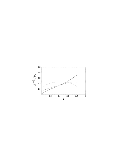
FIG. 9.: Model result for $H_{1}^{\perp(1/2)}/D_{1}$ (solid line) and comparison with the same ratio, where $H_{1}^{\perp(1/2)}$ is calculated according to Eq. (60) with $M_{C}=0.3$ GeV (dashed line) and $M_{C}=0.7$ GeV (dotted line).

Finally, we display in Fig. 10 the quantity

$$\frac{H_{1}^{\perp(1)}(z)}{D_{1}(z)}\equiv\frac{\pi}{D_{1}(z)}\int{\rm\,d}K_{{\scriptscriptstyle T}}^{2}\,\frac{K_{{\scriptscriptstyle T}}^{2}}{2z^{2}m_{\pi}^{2}}\,H_{1}^{\perp}(z,K_{{\scriptscriptstyle T}}^{2})\,,$$ (61)

because this ratio appears in the weighted asymmetries to be considered below. In Fig. 10, also the expression

$$\frac{\langle K_{{\scriptscriptstyle T}}^{2}\rangle(z)}{2z^{2}m_{\pi}^{2}}\frac{H_{1}^{\perp}(z)}{D_{1}(z)}=\pi\,\frac{H_{1}^{\perp}(z)}{D_{1}^{2}(z)}\int{\rm\,d}K_{{\scriptscriptstyle T}}^{2}\frac{K_{{\scriptscriptstyle T}}^{2}}{2z^{2}m_{\pi}^{2}}D_{1}(z,K_{{\scriptscriptstyle T}}^{2})\,$$ (62)

is shown for comparison. Once again, there is a remarkable agreement between the two different expressions, confirming the quite similar $K_{\scriptscriptstyle T}$ behaviour of $H_{1}^{\perp}$ and $D_{1}$.

FIG. 10.: Model result $H_{1}^{\perp(1)}/D_{1}$ (solid line) and comparison with the product $(\langle K_{{\scriptscriptstyle T}}^{2}\rangle/2z^{2}m_{\pi}^{2})(H_{1}^{\perp}/D_{1}^{\perp})$ (dashed line).

C Asymmetries in semi-inclusive DIS and $e^{+}e^{-}$ annihilation

We turn now to estimates of possible observables containing the Collins function. We will take into consideration one-particle inclusive DIS, where the Collins function appears in connection with the transversity distribution of the nucleon, and $e^{+}e^{-}$ annihilation into two hadrons belonging to two different jets.

In the first case, we consider the DIS cross section with a transversely polarized target and the production of one pion. We denote the transverse polarization vector of the target as $\vec{S}_{T}$. The cross section is differential in six variables, for which we choose $x,y,z,|\vec{P}_{h\perp}|,\phi^{S}_{h},\phi^{S}_{l}$, where $\vec{P}_{h\perp}$ is the transverse component of the pion momentum, $\phi^{S}_{h}$ is its azimuthal angle with respect to the target spin, and $\phi^{S}_{l}$ is the azimuthal angle of the lepton scattering plane again with respect to the target spin.

Orienting the spin of the target in two opposite directions and summing the cross sections we isolate the unpolarized part [14],

$${\rm\,d}^{6}\sigma_{U\uparrow}+{\rm\,d}^{6}\sigma_{U\downarrow}\;=\;\frac{4\alpha^{2}_{\rm em}}{sxy^{2}}\,\left(1-y+\frac{y^{2}}{2}\right)$$ (63)

$$\qquad\mbox{}\times\int{\rm\,d}^{2}\vec{p}_{{\scriptscriptstyle T}}{\rm\,d}^{2}\vec{k}_{{\scriptscriptstyle T}}\;\delta^{2}\left(\vec{p}_{{\scriptscriptstyle T}}-\frac{\vec{P}_{h\perp}}{z}-\vec{k}_{{\scriptscriptstyle T}}\right)$$ (65)

$$\qquad\mbox{}\times\sum_{a}e^{2}_{a}f_{1}^{a}(x,p_{{\scriptscriptstyle T}}^{2})\,D_{1}^{a}(z,z^{2}k_{{\scriptscriptstyle T}}^{2}),$$

where the subscript $U$ indicates an unpolarized electron beam, the index $a$ denotes quark flavours, and $f_{1}$ is the usual unpolarized quark distribution in the nucleon. Subtracting the cross sections we obtain the polarized part [14],

$${\rm\,d}^{6}\sigma_{U\uparrow}-{\rm\,d}^{6}\sigma_{U\downarrow}\;=\;-|\vec{S}_{T}|\,\frac{4\alpha_{\rm em}^{2}}{sxy^{2}}\,(1-y)\,\sin{(\phi_{h}^{S}-2\phi_{l}^{S})}$$ (66)

$$\mbox{}\times\int{\rm\,d}^{2}\vec{p}_{{\scriptscriptstyle T}}{\rm\,d}^{2}\vec{k}_{{\scriptscriptstyle T}}\;\delta^{2}\left(\vec{p}_{{\scriptscriptstyle T}}-\frac{\vec{P}_{h\perp}}{z}-\vec{k}_{{\scriptscriptstyle T}}\right)$$ (68)

$$\mbox{}\times\frac{\vec{P}_{h\perp}\cdot\vec{k}_{{\scriptscriptstyle T}}}{|\vec{P}_{h\perp}|\,m_{\pi}}\;\sum_{a}e^{2}_{a}h_{1}^{a}(x,p_{{\scriptscriptstyle T}}^{2})\,H_{1}^{\perp\,a}(z,z^{2}k_{{\scriptscriptstyle T}}^{2}).$$

Integration over the azimuthal angles would cause the polarized part of the cross section to vanish. After defining the angle $\phi\equiv\phi_{h}^{S}-2\phi_{l}^{S}$, we consider the $\sin\phi$ weighted transverse spin asymmetry

$$\left\langle\sin{\phi}\right\rangle_{UT}(x,y,z)$$ (69)

$$\qquad= \frac{\int{\rm\,d}\phi_{l}^{S}\,{\rm\,d}^{2}\vec{P}_{h\perp}\,\sin{\phi}\;({\rm\,d}^{6}\sigma_{U\uparrow}-{\rm\,d}^{6}\sigma_{U\downarrow})}{\int{\rm\,d}\phi_{l}^{S}\,{\rm\,d}^{2}\vec{P}_{h\perp}({\rm\,d}^{6}\sigma_{U\uparrow}+{\rm\,d}^{6}\sigma_{U\downarrow})}\,.$$ (70)

Inserting Eqs. (68,65) into the definition of the asymmetry results in an expression where the transverse momenta of $h_{1}$ and $H_{1}^{\perp}$ are still entangled in a convolution integral [28]. To resolve the convolution, it is required to assume a particular dependence of the transversity distribution on the intrinsic transverse momentum. The simplest example is

$$h_{1}(x,p_{{\scriptscriptstyle T}}^{2})\approx h_{1}(x)\,\frac{\delta(p_{{\scriptscriptstyle T}}^{2})}{\pi}\,,$$ (71)

that means supposing there is no intrinsic transverse momentum of the partons inside the target. Under this assumption, the pion transverse momentum with respect to the virtual photon is entirely due to the fragmentation process, i.e., $\vec{P}_{h\perp}=\vec{K}_{T}=-z\vec{k}_{T}$, and the convolution can be disentangled

$$\left\langle\sin{\phi}\right\rangle_{UT}(x,y,z)$$ (72)

$$\qquad\approx |\vec{S}_{{\scriptscriptstyle T}}|\frac{\frac{1}{xy^{2}}\,(1-y)\,\sum_{a}e_{a}^{2}\,h_{1}^{a}(x)\,H_{1}^{\perp(\frac{1}{2})a}(z)}{\frac{1}{xy^{2}}\left(1-y+\frac{y^{2}}{2}\right)\sum_{a}e_{a}^{2}\,f_{1}^{a}(x)\,D_{1}^{a}(z)}\,,$$ (73)

where the approximation sign reminds that the equality is assumption-dependent.

If we want to disentangle the convolution integral of Eq. (68) without making any assumption on the intrinsic transverse momentum distribution, we need to weight the integral with the magnitude of the pion transverse momentum [29]. This procedure results in the azimuthal transverse spin asymmetry

$$\bigg{\langle}\frac{|\vec{P}_{h\perp}|}{m_{\pi}}\sin{\phi}\bigg{\rangle}_{UT}(x,y,z)$$ (74)

$$\qquad= \frac{\int{\rm\,d}\phi_{l}^{S}{\rm\,d}^{2}\vec{P}_{h\perp}\,\frac{|\vec{P}_{h\perp}|}{m_{\pi}}\,\sin{\phi}\;({\rm\,d}^{6}\sigma_{U\uparrow}-{\rm\,d}^{6}\sigma_{U\downarrow})}{\int{\rm\,d}\phi_{l}^{S}{\rm\,d}^{2}\vec{P}_{h\perp}({\rm\,d}^{6}\sigma_{U\uparrow}+{\rm\,d}^{6}\sigma_{U\downarrow})}$$ (75)

$$\qquad= |\vec{S}_{{\scriptscriptstyle T}}|\frac{\frac{1}{xy^{2}}\,(1-y)\,z\,\sum_{a}e_{a}^{2}\,h_{1}^{a}(x)\,H_{1}^{\perp(1)a}(z)}{\frac{1}{xy^{2}}\,\left(1-y+\frac{y^{2}}{2}\right)\,\sum_{a}e_{a}^{2}\,f_{1}^{a}(x)\,D_{1}^{a}(z)}\;.$$ (76)

We achieved an assumption-free factorization of the $x$ dependent transversity distribution and the $z$-dependent Collins function. The measurement of this asymmetry requires to bin the cross section according to the magnitude of the pion transverse momentum. On the other side, this asymmetry represents potentially the cleanest method to measure the transversity distribution together with the Collins function. Moreover, it is not afflicted by complications due to Sudakov factors [30].

We show predictions for both transverse spin asymmetries defined in Eqs. (73) and (76). Different calculations can be found in the literature, e.g., in Refs. [31, 32, 27]. To estimate the magnitude of the asymmetries, we need inputs for the distribution functions, in particular for the transversity distribution. Several model calculations of this function are available at present (see [33] for a comprehensive review). We refrain ourselves from considering many different examples and rather restrict the analysis to two limiting situations. In the first case we adopt the non-relativistic assumption $h_{1}=g_{1}$, while in the second case we exhaust the upper bound on the transversity distribution, i.e., $h_{1}\leq\frac{1}{2}(f_{1}+g_{1})$ [34]. We use the simple parametrization of $g_{1}$ and $f_{1}$ suggested in [35]. At the moment, more sophisticated parametrizations are available, taking also scale evolution into account. However, all these parametrizations are compatible with each other to the extent of our purpose here, that is to give an estimate of the asymmetries for a low scale. We focus on the production of $\pi^{+}$, where the contribution of down quarks is negligible, not only because of the presence of unfavoured fragmentation functions, but also because the transversity distribution for down quarks is supposed to be much smaller than for up quarks.

In Fig. 11 we present the azimuthal asymmetry defined in Eq. (73) as a function of $x$, after integrating numerator and denominator over the variables $y$ and $z$, for the two cases described above. In Fig. 12, we present the same asymmetry as a function of $z$, after integrating over $y$ and $x$. As already mentioned before, our prediction is supposed to be valid at a low energy scale of about $1\,\rm{GeV}^{2}$. Neglecting evolution effects, it could be utilized for comparison with experiments at a scale of few GeV². We assume the value of the transverse polarization to be $|\vec{S}_{T}|=0.75$. In performing the integrations, we apply the kinematical cuts typical of the HERMES experiment, as described in [4]. Therefore, our prediction is particularly significant for HERMES, which is supposed to be the first experiment to measure this asymmetry. In principle, the simultaneous study of the $x$ and $z$-dependence of the asymmetry yields separate information on the distribution and fragmentation parts and allows to extract both up to a normalization factor [32]. Note, however, that this procedure relies on the assumption of up-quark dominance and is valid only if the asymmetry is truly factorized, so that the $x$-dependence can be ascribed entirely to the distribution functions and the $z$-dependence entirely to the fragmentation functions. Kinematical cuts could partially spoil this situation. We would like to stress that our calculation predicts an asymmetry up to the order of 10%, which should be within experimental reach, and suggests the possibility to distinguish between different assumptions on the transversity distribution.

FIG. 11.: Azimuthal transverse spin asymmetry $\langle\sin{\phi}\rangle_{UT}$ as a function of $x$. Solid line: assuming $h_{1}=g_{1}$. Dashed line: assuming $h_{1}=\frac{1}{2}(f_{1}+g_{1})$. The functions $f_{1}$ and $g_{1}$ are taken from [35].

FIG. 12.: Azimuthal transverse spin asymmetry $\langle\sin{\phi}\rangle_{UT}$ as a function of $z$. Solid line: assuming $h_{1}=g_{1}$. Dashed line: assuming $h_{1}=\frac{1}{2}(f_{1}+g_{1})$. The functions $f_{1}$ and $g_{1}$ are taken from [35].

Using the same procedure as before, we have estimated the asymmetry defined in Eq. (76), containing the weighting with $|\vec{P}_{h\perp}|/m_{\pi}$. The results are shown in Fig. 13 as a function of $x$ and in Fig. 14 as a function of $z$. The magnitude of this asymmetry is higher than in the unweighted case, which is due to the fact that the weighting spuriously enhances the asymmetry by about a factor two.

FIG. 13.: Azimuthal spin asymmetry $\langle\frac{|\vec{P}_{h\perp}|}{m_{\pi}}\,\sin{\phi}\rangle_{UT}$ as a function of $x$. Solid line: assuming $h_{1}=g_{1}$. Dashed line: assuming $h_{1}=\frac{1}{2}(f_{1}+g_{1})$. The functions $f_{1}$ and $g_{1}$ are taken from [35].

FIG. 14.: Azimuthal spin asymmetry $\langle\frac{|\vec{P}_{h\perp}|}{m_{\pi}}\,\sin{\phi}\rangle_{UT}$ as a function of $z$. Solid line: assuming $h_{1}=g_{1}$. Dashed line: assuming $h_{1}=\frac{1}{2}(f_{1}+g_{1})$. The functions $f_{1}$ and $g_{1}$ are taken from [35].

Besides appearing in semi-inclusive DIS in connection with the transversity distribution of the nucleon, the Collins function can be independently extracted from another process, that is electron-positron annihilation into two hadrons belonging to two back-to-back jets [36, 37]. We restrict ourselves to the case of $\gamma$-exchange only. In this process, one of the two hadrons (say hadron 2) defines the scattering plane together with the leptons and determines the direction with respect to which the azimuthal angles must be measured. The cross section is differential in five variables, e.g., $z_{1},z_{2},y,|\vec{P}_{h\perp}|,\phi$. The variables $z_{1}$ and $z_{2}$ are the longitudinal fractional momenta of the two hadrons. In the center of mass frame $y=(1+\cos{\theta})/2$, where $\theta$ is the angle of hadron 2 with respect to the momentum of the incoming leptons. The vector $\vec{P}_{h\perp}$ denotes the transverse component of the momentum of hadron 1 and $\phi$ is its azimutal angle with respect to the scattering plane. For a more detailed description of the kinematical variables we refer to [36, 37].

We define the azimuthal asymmetry

$$\left\langle P_{h\perp}^{2}\cos{2\phi}\right\rangle_{e^{+}e^{-}}(\theta,z_{1},z_{2})$$ (77)

$$= \frac{\int{\rm\,d}^{2}\vec{P}_{h\perp}\,P_{h\perp}^{2}\,\cos{2\phi}\;{\rm\,d}^{5}\sigma_{e^{+}e^{-}}}{\int{\rm\,d}^{2}\vec{P}_{h\perp}\,P_{h\perp}^{2}\,{\rm\,d}^{5}\sigma_{e^{+}e^{-}}}$$ (78)

$$= \frac{2\,\sin^{2}{\theta}}{1+\cos^{2}{\theta}}\,\frac{H_{1}^{\perp(1)}(z_{1})\,\bar{H}_{1}^{\perp(1)}(z_{2})}{\left(D_{1}(z_{1})\,\bar{D}_{1}^{(1)}(z_{2})+D_{1}^{(1)}(z_{1})\,\bar{D}_{1}(z_{2})\right)},$$ (79)

where summations over quark flavours are understood. The weighting with a second power of $P_{h\perp}$ in the numerator is necessary to obtain a deconvoluted expression. We prefer to use the same weighting in the denominator as well, to avoid a modification of the asymmetry just caused by the weighting.

In Fig. 15 we present the estimate of the asymmetry defined above, entirely based on our model. The asymmetry has been integrated over $z_{2}$ and $\theta$, leaving the dependence on $z_{1}$ alone. We have extended the $\theta$ integration interval all the way to $[0,\pi]$, to obtain a conservative estimate. In fact, limiting the interval to $[\frac{\pi}{4},\frac{3\pi}{4}]$ will enhance the asymmetry by a factor 2, approximately. Because the Collins function increases with increasing $z$, we also get a larger asymmetry by restricting the integration range for $z_{2}$. As an illustration of this feature, in Fig. 15 we present two results, obtained from two different integration ranges. Our prediction is supposed to be valid only at low energy scales and should be evolved for comparison with higher energy experiments. It is important to note that we estimate the asymmetry to be of the order of about 5%, and thus should be very well observable in experiments.

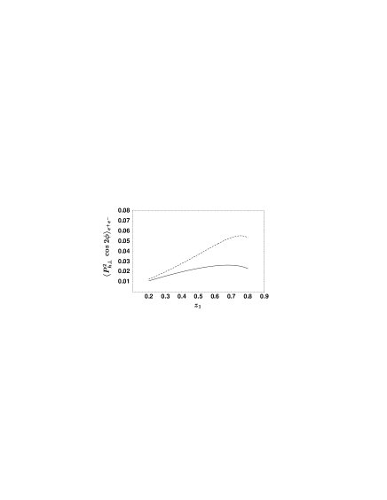
FIG. 15.: Azimuthal asymmetry $\langle P_{h\perp}^{2}\cos{2\phi}\rangle_{e^{+}e^{-}}$ for $e^{+}e^{-}$ annihilation into two hadrons, integrated over the range $0.2\leq z_{2}\leq 0.8$ (solid line), and over the range $0.5\leq z_{2}\leq 0.8$ (dashed line).

IV Summary and conclusions

We have estimated the Collins fragmentation function for pions at a low energy scale by means of the Manohar-Georgi model. This model contains three essential features of non-perturbative QCD: massive quark degrees of freedom, chiral symmetry and its spontaneous breaking (with pions as Goldstone bosons). Because of the chiral invariant interaction between pions and quarks, the fragmentation process can be evaluated in a perturbative expansion. The constituent quark mass, the axial pion-quark coupling $g_{\scriptscriptstyle A}$ and the maximum virtuality $\mu^{2}$ of the fragmenting quark are free parameters of our approach. The quark mass and $g_{\scriptscriptstyle A}$ are constrained within reasonable limits. To ensure the convergence of the chiral perturbation expansion, $\mu^{2}$ cannot exceed a typical hadronic scale. We have mostly considered the value $\mu^{2}=1\,\rm{GeV}^{2}$, which guarantees that the momenta of the particles produced in the fragmentation process stay well below the scale of chiral symmetry breaking, $\Lambda_{\chi}\approx 1$ GeV. To determine the appropriate value of $\mu^{2}$, the average transverse momentum of a data set could be used. In any case, we observed that variations of the free parameters within reasonable limits have only a minor influence on the shape of the results, implying that our approach has a strong predictive power for the $z$-behaviour of the various functions.

We have found that the Manohar-Georgi model reproduces reasonably well the unpolarized pion fragmentation function and the average transverse momentum of a produced hadron as function of $z$, supporting the idea of describing the fragmentation process by a chiral invariant approach.

Compared to the unpolarized fragmentation function, modeling the Collins function is considerably more difficult, mainly because of its chiral-odd and time-reversal odd nature. In our approach, the helicity-flip required to generate a chiral-odd object is caused by the mass of the constituent quark, while the T-odd behaviour is produced via one-loop corrections. The Collins function exhibits a quite distinct behaviour from the the unpolarized fragmentation function. In particular, the ratio $H_{1}^{\perp}/D_{1}$ is strongly increasing with increasing $z$.

On the basis of our results, we have calculated the transverse single-spin asymmetry in semi-inclusive DIS where the Collins function appears in combination with the transversity of the nucleon. This observable will be measured in the near future at HERMES and could also be investigated at COMPASS, Jlab (upgraded) and eRHIC. For typical HERMES kinematics the asymmetry is of the order of $10\%$, giving support to the intention of extracting the nucleon transversity in this way. We believe that our estimate of the Collins function, despite its uncertainties, can be very useful for this extraction.

More information on the Collins function from the experimental side is urgently required. In this respect, the most promising experiment seems to be $e^{+}e^{-}$ annihilation into two hadrons, where $H_{1}^{\perp}$ appears squared in an azimuthal $\cos{2\phi}$ asymmetry. According to our calculation, an asymmetry of the order of $5\%$ can be expected, which should be measurable at high luminosity accelerators, such as BABAR and BELLE. Dedicated measurements of the Collins function would be extremely important for the extraction of the transversity distribution. Moreover, they could answer the question whether a chiral invariant Lagrangian can be used to model the Collins function.

- [1] J. Collins, Nucl. Phys. B396 (1993) 161 [hep-ph/9208213].
- [2] A. Bacchetta, R. Kundu, A. Metz and P. J. Mulders, Phys. Lett. B 506 (2001) 155 [hep-ph/0102278].
- [3] X. Artru, J. Czyzewski and H. Yabuki, Z. Phys. C 73 (1997) 527 [hep-ph/9508239].
- [4] A. Airapetian et al. [HERMES Collaboration], Phys. Rev. Lett. 84 (2000) 4047 [hep-ex/9910062].
- [5] A. Airapetian et al. [HERMES Collaboration], Phys. Rev. D 64 (2001) 097101 [hep-ex/0104005].
- [6] M. Anselmino, M. Boglione and F. Murgia, Phys. Rev. D 60 (1999) 054027 [hep-ph/9901442].
- [7] M. Boglione and E. Leader, Phys. Rev. D 61 (2000) 114001 [hep-ph/9911207].
- [8] A. V. Efremov, K. Goeke and P. Schweitzer, Phys. Lett. B 522 (2001) 37 [hep-ph/0108213].
- [9] A. Manohar and H. Georgi, Nucl. Phys. B 234 (1984) 189.
- [10] X. D. Ji and Z. K. Zhu, hep-ph/9402303.
- [11] J. Czyzewski, Acta Phys. Polon. 27 (1996) 1759 [hep-ph/9606390].
- [12] S. Weinberg, PhysicaA 96, 327 (1979).
- [13] J. Levelt and P. J. Mulders, Phys. Lett. B 338 (1994) 357 [hep-ph/9408257].
- [14] P. J. Mulders and R. D. Tangerman, Nucl. Phys. B461 (1996) 197 [hep-ph/9510301], and Nucl. Phys. B484 (1997) 538 (E).
- [15] S. Weinberg, Phys. Rev. Lett. 65, 1181 (1990).
- [16] S. Boffi, L. Y. Glozman, W. Klink, W. Plessas, M. Radici and R. F. Wagenbrunn, hep-ph/0108271.
- [17] S. Kretzer, Phys. Rev. D 62 (2000) 054001 [hep-ph/0003177].
- [18] B. A. Kniehl, G. Kramer and B. Pötter, Nucl. Phys. B 582 (2000) 514 [hep-ph/0010289].
- [19] L. Bourhis, M. Fontannaz, J. P. Guillet and M. Werlen, Eur. Phys. J. C 19 (2001) 89 [hep-ph/0009101].
- [20] S. Kretzer, E. Leader and E. Christova, Eur. Phys. J. C 22 (2001) 269 [hep-ph/0108055].
- [21] P. Abreu et al. [DELPHI Collaboration], Z. Phys. C 73 (1996) 11.
- [22] A. Bacchetta, M. Boglione, A. Henneman and P. J. Mulders, Phys. Rev. Lett. 85 (2000) 712 [hep-ph/9912490].
- [23] A. Bacchetta, M. Boglione, A. Henneman and P. J. Mulders, hep-ph/0005140.
- [24] K. A. Oganessyan, H. R. Avakian, N. Bianchi and A. M. Kotzinian, hep-ph/9808368;
- [25] A. M. Kotzinian, K. A. Oganessyan, H. R. Avakian and E. De Sanctis, Nucl. Phys. A666&667 (2000) 290c [hep-ph/9908466].
- [26] E. De Sanctis, W. D. Nowak and K. A. Oganessyan, Phys. Lett. B 483, 69 (2000) [hep-ph/0002091].
- [27] B. Q. Ma, I. Schmidt and J. J. Yang, hep-ph/0110324.
- [28] J. P. Ralston and D. E. Soper, Nucl. Phys. B 152 (1979) 109.
- [29] A. M. Kotzinian and P. J. Mulders, Phys. Lett. B 406 (1997) 373 [hep-ph/9701330].
- [30] D. Boer, Nucl. Phys. B 603 (2001) 195 [hep-ph/0102071].
- [31] M. Anselmino and F. Murgia, Phys. Lett. B 483 (2000) 74 [hep-ph/0002120].
- [32] V. A. Korotkov, W. D. Nowak and K. A. Oganessyan, Eur. Phys. J. C 18 (2001) 639 [hep-ph/0002268].
- [33] V. Barone, A. Drago and P. G. Ratcliffe, Phys. Rept. 359 (2002) 1 [hep-ph/0104283].
- [34] J. Soffer, Phys. Rev. Lett. 74 (1995) 1292 [hep-ph/9409254].
- [35] S. J. Brodsky, M. Burkardt and I. Schmidt, Nucl. Phys. B 441 (1995) 197 [hep-ph/9401328].
- [36] D. Boer, R. Jakob and P. J. Mulders, Nucl. Phys. B 504 (1997) 345 [hep-ph/9702281].
- [37] D. Boer, R. Jakob and P. J. Mulders, Phys. Lett. B424 (1998) 143 [hep-ph/9711488].