Abstract

Recent developments and open issues in chiral dynamics with strange quarks are reviewed. Topics include: Order parameters of chiral symmetry breaking, the flavor dependence of these order parameters, speculations about the phase structure of QCD with varying number of flavors, OZI violation and its natural emergence in case of a small strange quark condensate, heavy kaon chiral perturbation theory, an update on pion-pion, pion-kaon and pion-nucleon sigma terms, the dynamics and nature of scalar mesons, the role of the scalar pion and kaon form factors, attempts to describe some strange baryons employing coupled channel dynamics tied to unitarity and chiral perturbation theory, and the role of final state interactions in Goldstone boson pair production in proton-proton collisions.

PACS: 12.39.Fe, 14.40.Aq, 12.38.Aw, 11.30.Rd

1 Introduction

The strange quark plays a special role in the QCD dynamics at the confinement scale. In this essay, I will discuss some open questions surrounding chiral dynamics with strange quarks, pertinent to the structure of the strong interaction vacuum as well as to the structure of light mesons and baryons. Some of these questions are:

• Is the strange quark really light? It is well established that the up and the down quarks are light compared to any hadronic scale, in particular $m_{u},m_{d}\ll\Lambda_{\rm QCD}$, with $\Lambda_{\rm QCD}\simeq 150\,$MeV. On the other hand, $m_{s}\sim\Lambda_{\rm QCD}$ (the most recent non-lattice determination based on scalar sum rules gives $m_{s}(2\,{\rm GeV})=99\pm 16\,$MeV [1]. See that paper for many more references on determinations of $m_{s}$.) Therefore, one can even entertain the extreme possibility of considering the strange quark as heavy. Still, there are many successes of standard three flavor chiral perturbation theory based on the conventional scenario which treats the strange quark mass as a perturbation on equal footing with the light quark masses $m_{u}$ and $m_{d}$ (see e.g. the contributions of Ametller [2], Bijnens [3], Gasser [4] and Holstein [5] to this volume).

• Why is the OZI rule so badly violated in the scalar sector with vacuum quantum numbers? This rule is exact in the limit of a large number of colors $N_{c}\to\infty$ and works astonishingly well in most channels even for $N_{c}=3$, i.e. in nature. However, in the $0^{++}$ channel, huge deviations from the OZI rule are observed. One example is the reaction $J/\Psi\to\phi\pi\pi/\bar{K}K$, which is OZI suppressed to leading order (see Fig. 1a) but has an additional doubly OZI suppressed contribution depicted in Fig. 1b. These processes have been measured at DM2 and Mark-III. The $\pi^{+}\pi^{-}$ event distribution shows a clear peak at the energy of 980 MeV which is due to the $f_{0}$ scalar meson. This lets one anticipate that the dynamics of the low-lying scalar mesons and the mechanism of OZI violation are in some way related.

  Figure 1: Quark line diagrams for decay $J/\Psi$ into the $\phi$ and a meson pair ($\pi\pi$ or $K\bar{K}$). The quark flavors are explicitly given, $n$ refers to the light non–strange $u,d$ quarks. The hatched blob in a) depicts the final state interactions in the coupled $\pi\pi/K\bar{K}$ system.

• More generally, it is of interest to learn about the phase structure of SU($N_{c}$) gauge theory at large number of flavors $N_{f}\,$. In QCD, we know that asymptotic freedom is lost for $N_{f}\geq 17$ but from the study of the two-loop $\beta$ function one expects that there is a conformal window around $N_{f}\simeq 6$, see [6] and for a recent update with many references, see [7]. This lets one contemplate the question whether there is already a rich phase structure even for the transition from $N_{f}=2$ to $N_{f}=3$ ? Some lattice studies seem to indicate a strong flavor sensitivity when going from $N_{f}=2$ to $N_{f}=4$. In Fig. 2 I show some results obtained by the Columbia group using staggered fermions. These seem to indicate a suppression of the chiral condensate as the number of flavors is increased together with the degeneracy of meson and baryon states of opposite parity [8]. For similar lattice results, see [9].

  Figure 2: Left panel: Suppression of the chiral condensate with increasing number of flavors. Right panel: Degeneracy of staggered hadron masses for $N_{f}=4$ which seems to indicate a restoration of chiral symmetry. From the QCDSP collaboration.

• The so-called sigma terms play a special role in the investigations of chiral dynamics chiefly because they are nothing but the expectation values of the quark mass term of QCD within hadron states, $H$, $\langle H|m_{q}\bar{q}q|H\rangle$, with $H$ e.g. pions, kaons or nucleons. Since no external scalar probes are available, the determination of these matrix elements proceeds by analyzing four–point functions, more precisely Goldstone boson–hadron scattering amplitudes in the unphysical region, $\phi(q)+H(p)\to\phi(q^{\prime})+H(p^{\prime})$ (note that the hadron can also be a Goldstone boson). While the pion and kaon sigma terms behave as expected, there is still much debate about the pion-nucleon sigma term, especially concerning the possible admixture of $\bar{s}s$ pairs in the proton’s wave function (which itself can, of course, not be measured). This might be taken as a hint that the transition from two to three flavors reveals some unexpected behavior.

• The nature of the low-lying scalar mesons, the so-called “sigma”, the $f_{0}(980)$, $a_{0}(980)$ and so on, is still under debate - are these quark-antiquark states, kaon-antikaon molecules or dynamically generated by the strong final state interactions in the coupled channel $\pi\pi/\bar{K}K$ system? Is there furthermore a mixing of some of these states with glueballs ? To my opinion, any model to describe these states must be able to describe the large body of data on decays (strong and electromagnetic) as well as scattering and production reactions. Also, since these particles have vacuum quantum numbers, they play a special role as we already encountered in the brief discussion of OZI violation and the phase structure of QCD for more than two flavors.

• In the baryon sector, there are also some “strange” states with non-vanishing strangeness. More precisely, what is the nature of some strange baryons like the $\Lambda(1405)$ or the $S_{11}(1535)$, are these three quarks states or meson-baryon bound states ? The latter scenario was already contemplated many years ago by Dalitz and Tuan [10] and has been rejuvenated with the advent of coupled channel calculations using chiral Lagrangians to specify the driving interaction. The bound-state scenario is triggered by the fact that the $\Lambda(1405)$ sits just above/below the $\pi\Sigma/\bar{K}N$ threshold as shown in Fig. 3.

  Figure 3: Location of the $\Lambda(1405)$ between the $\pi\Sigma$ and the $\bar{K}N$ thresholds.

This essay is organized as follows. In section 2 I briefly discuss the chiral symmetry of QCD and its breaking with particular emphasis on the pertinent order parameters. Section 3 discusses QCD inequalities for these order parameters as a function of $N_{f}$, the number of light quark flavors. Further facts and speculations about the flavor dependence of the quark condensate are collected in section 4. The reordering of the chiral expansion in light of a possible suppression of the three flavor quark condensate is discussed in section 5. Another type of reordering based on the assumption that one can treat kaons and etas has heavy particles is presented in section 6 and some pertinent results are discussed. Then, in section 7 the status of sigma terms as extracted from pion-pion, pion-kaon and pion-nucleon scattering is reviewed. Some remarks on the structure of the light scalar mesons and certain strange baryons are made in sections 8 and 9, respectively. Finally, I will make some comments about pseudoscalar (strange) meson production in proton-proton collisions in section 10. The essay concludes with a short summary and outlook in section 11.

2 Chiral symmetry of QCD - order parameters

The QCD Lagrangian has the form

$${\cal L}_{\rm QCD}=-\frac{1}{4}G_{\mu\nu}^{\alpha}G^{\mu\nu,\alpha}-\frac{g^{2}}{32\pi^{2}}{\theta}\tilde{G}_{\mu\nu}^{\alpha}{G}^{\mu\nu,\alpha}+\sum_{q}\bar{q}(iD\!\!\!\!/-m_{q})q+\sum_{Q}\bar{Q}(iD\!\!\!\!/-M_{Q})Q+{\cal L}_{\rm gf}~{},$$ (2.1)

with $G_{\mu\nu}^{\alpha}$ the conventional gluon field strength tensor, $\tilde{G}_{\mu\nu}^{\alpha}$ its dual, the color index $\alpha$ runs from 1 to 8, $g$ denotes the strong coupling constant, $D\!\!\!\!/=\gamma^{\mu}D_{\mu}=\gamma^{\mu}(\partial_{\mu}-igG_{\mu}^{\alpha}T^{\alpha})$ the gauge-covariant derivative (with $T^{\alpha}=\lambda^{\alpha}/2$ the SU(3) generators), $q$ collects the light quark fields $u$, $d$, and $s$ whereas the heavy quarks $c$, $b$ and $t$ are collected in $Q$. These fields are chosen such that the current quark mass matrix is diagonal, its entries are the three real numbers $m_{q}$ and the three $M_{Q}$. The topological term involving the dual field strength tensor leads to strong $P$ and $T$ violation. Experimental bounds like from the electric dipole moment of the neutron, however, force the vacuum angle $\theta$ to be very tiny. Therefore, in what follows, we set the $\theta$ angle to zero. The term ${\cal L}_{\rm gf}$ collects gauge–fixing and ghost terms. The heavy quark sector is governed by the so-called heavy quark symmetry, which allows for many interesting predictions. The light quark sector, on the other hand, is dominated by the so-called chiral symmetry, as will be explained shortly. We will consider the heavy quarks as infinitely heavy, that is they decouple from the light quark sector. Of course, there are interesting processes which show an intricate interplay between heavy quark and chiral symmetry, but we will not be concerned with these here. To a good first approximation, one can set the light quark masses to zero, $m_{q}=0$. In that case the quark fields can be decomposed into right- and left-handed parts, which do not interact. Stated differently, one can independently rotate the right- and the left-handed light quark fields,

$$q_{R/L}\to V_{R/L}\,q_{R/L}~{},\quad V_{R/L}\in{\rm SU}(3)_{R/L}~{}.$$ (2.2)

Obviously, a fermion mass term like $\bar{q}_{L}{\cal M}q_{R}+\bar{q}_{R}{\cal M}^{\dagger}q_{L}$ breaks this chiral symmetry, but it can still be considered an approximate symmetry if the quark masses are in some sense light. Chiral symmetry leads to eight conserved right- and eight left-handed currents. Alternatively, one consider eight conserved vector ($V=L+R$) and eight conserved axial-vector ($A=L-R$) currents and the corresponding conserved charges:

$$\begin{array}[]{llllll}\partial^{\mu}V_{\mu}^{a}&=&i\bar{q}[{\cal M},\lambda^{a}]q&\rightarrow&Q_{V}^{a}=\int_{V}d^{3}V_{0}^{a}&{\rm with}~{}~{}\displaystyle{{dQ_{V}^{a}\over dt}}=0~{},\\ \\ \partial^{\mu}A_{\mu}^{a}&=&i\bar{q}\{{\cal M},\lambda^{a}\}\gamma_{5}q&\rightarrow&Q_{A}^{a}=\int_{V}d^{3}V_{0}^{a}&{\rm with}~{}~{}\displaystyle{{dQ_{A}^{a}\over dt}}=0~{},\end{array}$$

with $a=1,\ldots,8$ and ${\cal M}={\rm diag}(m_{u},m_{d},m_{s})$ the diagonal current quark matrix. In three flavor chiral limit, that is $m_{u}=m_{d}=m_{s}=0$, these 16 currents and charges are exactly conserved. It is believed that QCD undergoes spontaneous chiral symmetry breaking and that the symmetry is realized in the Nambu-Goldstone mode, i.e.

$$\lim_{V\to\infty}\langle 0|[{\cal O},Q_{V}^{a}]|0\rangle=0~{},\quad{\rm but:}\quad\lim_{V\to\infty}\langle 0|[{\cal O},Q_{A}^{a}]|0\rangle\neq 0~{},$$ (2.3)

where ${\cal O}$ is some order parameter (as discussed in more detail below) and $|0\rangle$ denotes the highly complicated strong interaction vacuum. It is one of the few exact theorems of QCD that in the absence of $\theta$-terms, the vector symmetry cannot be broken (more generally this holds for any vector-like gauge theory under the stated assumptions) [11]. There is also ample phenomenological evidence that the axial symmetry is not realized in nature. For example, the hadron spectrum reveals SU(3)_V multiplets (the celebrated eightfold way), but no parity doublets, as it would be the case for an additional realized axial symmetry, are observed. The axial symmetry is hidden, its dynamics is transfered into the interactions of the Goldstone bosons, which are a consequence of the symmetry violation. In massless QCD, there are eight of these modes and they should be massless. Collectively, I denote these degrees of freedom as pions. As a direct consequence of Goldstone’s theorem, these pions can couple to the vacuum via the axial current,

$$\langle 0|A_{\mu}^{a}(x)|\pi^{b}(p)\rangle=i\delta^{ab}F(3)p_{\mu}{\rm e}^{ip\cdot x}~{},$$ (2.4)

with $F(3)$ the pion decay constant in the three flavor chiral limit, i.e.

$$\lim_{m_{u},m_{d},m_{s}\to 0}F_{\pi}=F(3)~{}.$$ (2.5)

In the real world, that is massive QCD, these Goldstone bosons can be identified with the three pions ($\pi^{+},\pi^{-},\pi^{0}$), the four kaons ($K^{+},K^{-},K^{0},\bar{K}^{0}$) and the eta ($\eta$). They are the lightest hadrons and their finite mass is related to the small current quark masses. We will come back to this topic in section 4.

Let me return to the notion of an order parameter. A textbook example is a magnetic system of spins located on some lattice sites interacting with an energy $\sim\vec{S}_{i}\cdot\vec{S}_{j}$, where $i$ denotes some site and $j$ belongs to its nearest neighbors. Obviously, the magnet Hamiltonian is invariant under spatial rotations, i.e under O(3). However, below the Curie temperature this symmetry is spontaneously broken, O(3) $\to$ O(2), with all spins pointing in one direction as shown in panel a) of Fig. 4.

Figure 4: a) Ferromagnetic order. The spins on all lattice sites point in the same direction. This defines the magnetization. b) Anti–ferromagnetic order. There are two sublattices as shown by the solid and dashed lines. The spins on the sites of these sublattices point in opposite directions, such that the total magnetization vanishes.

This defines the magnetization $\vec{M}$, and one has $\langle 0|\vec{M}|0\rangle\neq 0$, where $|0\rangle$ denotes the ground state. The remaining O(2) symmetry group is given by the rotations around the direction of the magnetization. More generally, one defines an order parameter ${\cal O}$ by the relation:

$$\langle 0|{\cal O}|0\rangle\neq 0\quad\rightarrow\quad{\rm spontaneous}~{}~{}{\rm symmetry}~{}~{}{\rm breaking}~{}.$$ (2.6)

For the ferromagnet, the magnetization is the simplest order parameter, in fact, there is an infinite amount of such order parameters. For the ferromagnetic case, any positive power of $\vec{M}$ qualifies as such. The inverse of Eq. (2.6) is, however, not true. This can be easily exemplified using an anti-ferromagnetic system, as shown in the panel b) of Fig. 4. Here, the total magnetization is zero, because there are two sublattices, on which the spins point in opposite direction, as shown in the figure by the dashed and the solid lines. The pertinent order parameter in this case is $\vec{M}_{\rm solid}-\vec{M}_{\rm dashed}$, where the magnetization is defined on the corresponding sublattices. More complicated order parameters, which account for this underlying structure, can of course be considered. From this simple example one concludes that a detailed study of the order parameters in a given system can reveal the nature of the mechanism of the spontaneous symmetry breaking.

Now the question arises what are the order parameters of the spontaneous chiral symmetry breaking ? Consider first the current-current correlator between vector and axial currents,

$$\Pi^{ab}_{\mu\nu}(q) = i\int d^{4}x\,{\rm e}^{iqx}\,\langle 0|T\{V_{\mu}^{a}(x)V_{\nu}^{b}(0)-A_{\mu}^{a}(x)A_{\nu}^{b}(0)\}|0\rangle$$ (2.7)

$$= 4i\int d^{4}x\,{\rm e}^{iqx}\,\langle 0|T\{R_{\mu}^{a}(x)L_{\nu}^{b}(0)\}|0\rangle~{}.$$

In the three flavor chiral limit, it can be written in terms of meson and continuum contributions, i.e. for $m_{q}\to 0$ we have

$$\Pi^{ab}_{\mu\nu}(q)=(q_{\mu}q_{\nu}-g_{\mu\nu}q^{2})\,\left[-\sum_{P}{F^{2}(3)\over q^{2}}-\sum_{V}{F_{V}^{2}\over M_{V}^{2}-q^{2}}+\sum_{A}{F_{A}^{2}\over M_{A}^{2}-q^{2}}+\ldots\right]~{},$$ (2.8)

where the first sum runs over the pseudoscalar Goldstone bosons, the second over vector and the third over axial-vector mesons. It follows immediately that

$$\Pi^{ab}_{\mu\nu}(0)=-\frac{1}{4}g_{\mu\nu}\delta^{ab}F^{2}(3)~{}.$$ (2.9)

We have thus identified an order parameter of spontaneous chiral symmetry breaking (S$\chi$SB), namely the pion decay constant in the chiral limit. Its non-vanishing is a sufficient and necessary condition for S$\chi$SB,

$$\Pi^{ab}_{\mu\nu}(0)\neq 0\leftrightarrow F(3)\neq 0\leftrightarrow{\rm S}\chi{\rm SB}~{}.$$ (2.10)

Naturally, there are many other possible order parameters, often considered is the light quark condensate,

$$\langle 0|\bar{q}q|0\rangle=\langle 0|\bar{u}u|0\rangle^{(3)}=\langle 0|\bar{d}d|0\rangle^{(3)}=\langle 0|\bar{s}s|0\rangle^{(3)}\equiv-\Sigma(3)~{},$$ (2.11)

because the scalar-isoscalar operator $\bar{q}q$ mixes right- and left-handed quark fields. As will be discussed in the following sections, the quark condensate plays a different role than the pion decay constant. Other possible color-neutral order parameters of higher dimension are e.g. the mixed quark–gluon condensate $\langle 0|\bar{q}^{i}\sigma^{\mu\nu}G_{\mu\nu}^{\alpha}T^{\alpha}_{ij}q_{j}|0\rangle^{(3)}$ or certain four-quark condensates $\langle 0|(\bar{q}\Gamma_{1}q)(\bar{q}\Gamma_{2}q)|0\rangle$ with $\Gamma_{i}$ some Dirac operator. This concludes our general discussion of order parameters in QCD. It goes without saying that the spontaneously and explicitely broken chiral symmetry can be systematically analyzed in terms of an effective field theory - chiral perturbation theory (CHPT) (or some variant thereof) [12, 13, 14].

3 QCD inequalities: Flavor dependence of chiral order parameters

We now consider some exact results for the flavor dependence of order parameters of the S$\chi$SB in QCD. For this, we consider QCD on a torus, or in an Euclidean ($t\to-ix^{0}$) box of size $L\times L\times L\times L$, understanding of course that we have to take the infinite volume limit $L\to\infty$ at its appropriate place. Quarks and gluon fields are then subject certain boundary conditions, which are anti-periodic and periodic, in order. I will not go through the derivation of these results, but rather refer to the work of Banks and Casher [15], Vafa and Witten [11], Leutwyler and Smilga [16], Stern [17] and Descotes, Girlanda and Stern [18] (and others). The interested reader is referred to these articles for the details.

To be specific, consider the Dirac operator of QCD in a gluonic background,

$${\cal D}[G]=\gamma_{\mu}(\partial_{\mu}+iG_{\mu})={\cal D}^{\dagger}[G]~{},$$ (3.1)

where the important hermiticity property is rooted in the Euclidean metric we are using. The eigenvalue equation for the Euclidean Dirac operator reads

$${\cal D}\!\!\!\!/\,\psi_{n}=\lambda_{n}\,\psi_{n}~{}.$$ (3.2)

From this, three important observations can be made. First, the spectrum of ${\cal D}[G]$ is symmetric under $\psi_{n}\to\gamma_{5}\psi_{n}$, that is we can classify the eigenvalues $\lambda_{n}\geq 0$ by a strictly positive, increasing number (since $\lambda_{-n}=-\lambda_{n}$). In addition, for gauge fields with non-vanishing winding number $\nu$, the spectrum contains $|\nu|$ topological zero modes. Second, one can derive an uniform upper bound for the small eigenvalues [11],

$$|\lambda_{n}[G]|<C\,{n^{1/d}\over L}\equiv\omega_{n}~{},$$ (3.3)

where $d$ is the dimensionality of space-time and the constant $C$ does not depend on the gauge field configuration, the integer $n$ and the volume $V=L^{d}$ but only on the shape of the space-time manifold (at fixed volume). Third, only the small eigenvalues are relevant to generate S$\chi$SB in the infinite volume limit (see below). Consider now some operator for varying number of flavors, more specifically for the transition $N_{f}\to N_{f}+1$. The flavor dependence of such an operator enters through the quark propagator,

$$S(x,y|G)=\sum_{n}{\psi_{n}(x)\psi_{n}^{\dagger}(y)\over{\cal M}+i\lambda_{n}}~{},$$ (3.4)

and through the fermion determinant. More precisely, consider first the quark condensate for $N_{f}$ flavors with a uniform light mass $m$ in a gluonic background,

$$\Sigma(N_{f})=\lim_{L\to\infty}{1\over L^{4}}\left\langle\int d^{4}x\,{\rm Tr}\,S(x,x|G)\right\rangle_{[G]}^{N_{f}} = \lim_{L\to\infty}{1\over L^{4}}\left\langle\sum_{n}{\psi_{n}(x)\psi_{n}^{\dagger}(x)\over m+i\lambda_{n}}\right\rangle_{[G]}^{N_{f}}$$ (3.5)

$$= \lim_{L\to\infty}{1\over L^{4}}\left\langle\sum_{n}{m\over m^{2}+\lambda_{n}^{2}}\right\rangle_{[G]}^{N_{f}}$$

$$= \lim_{m\to 0}\int_{-\infty}^{+\infty}d\epsilon{m\over m^{2}+\epsilon^{2}}\,\lim_{L\to\infty}{1\over L^{4}}\Biggl{\langle}\underbrace{\sum_{n}\delta(\epsilon-\lambda_{n})}_{\equiv\rho(\epsilon,L)}\Biggr{\rangle}_{[G]}^{N_{f}}~{},$$

where the symbol $\langle~{}\rangle_{[G]}^{N_{f}}$ represents the normalized average over gauge field configurations weighted by the fermion determinant,

$$\left\langle O\right\rangle_{[G]}^{N_{f}}=Z^{-1}\int d\mu[G]\,O\,\Delta^{N_{f}}(m|G)\,\prod_{j>N_{f}}\Delta(m_{j}|G)\,\exp(-S[G])~{}.$$ (3.6)

Here, $S[G]$ stands for the Yang-Mills action and $Z$ ia a normalization constant. This functional integral may also be viewed as an average over all Dirac spectra. Note that Eq. (3.5) is nothing but the Banks-Casher relation [15]

$$\Sigma(N_{f})=\pi\,\lim_{\epsilon\to 0}\lim_{L\to\infty}\rho(\epsilon,L)~{},$$ (3.7)

which expresses the quark condensate in terms of the zero modes of the QCD Dirac operator. From this formula one concludes that an accumulation of small eigenvalues $|\lambda_{n}|\sim 1/L^{4}$ is necessary so that $\Sigma(N_{f})\neq 0$. A similar relation can be obtained for the pion decay constant [17]

$$F^{2}(N_{f})=\lim_{L\to\infty}{1\over L^{4}}\left\langle\sum_{k,n}{m\over m^{2}+\lambda_{k}^{2}}{m\over m^{2}+\lambda_{n}^{2}}J_{kn}\right\rangle_{[G]}^{N_{f}}~{},$$ (3.8)

in terms of the “quark mobility”

$$J_{kn}=\frac{1}{4}\sum_{\mu}\left|\int d^{4}x\,\psi^{\dagger}_{n}(x)\gamma_{\mu}\psi_{n}(x)\right|^{2}~{}.$$ (3.9)

This can be brought in a form similar to the Banks-Casher relation, Eq. (3.7),

$$F^{2}(N_{f})=\pi^{2}\,\lim_{\epsilon\to 0}\lim_{L\to\infty}L^{4}\,J(\epsilon,L)\,\rho^{2}(\epsilon,L)~{}.$$ (3.10)

Clearly, an accumulation of small eigenvalues $|\lambda_{n}|\sim 1/L^{2}$ is necessary so that $F^{2}\neq 0$. We note the different IR sensitivity as compared to the quark condensate. Now we return to Eq. (3.6). The existence of the bound Eq. (3.3) allows to split the fermion determinant into IR and UV parts [19] by choosing a cut-off $\Lambda$ and an integer $K$ such that $\omega_{K}=\Lambda$. The single flavor fermion determinant takes the form

$$\Delta(m|G)=m^{|\nu|}\,\Delta_{\rm IR}(m|G)\,\Delta_{\rm UV}(m|G)~{},$$ (3.11)

where $\Delta_{\rm IR}$ involves the first $K$ non-zero eigenvalues and it is bounded by one,

$$\Delta_{\rm IR}(m|G)=\prod_{k=1}^{K}{m^{2}+\lambda_{k}^{2}[G]\over m^{2}+\omega_{k}^{2}}<1~{}.$$ (3.12)

Consequently, since the order parameters $F^{2}$ and $\Sigma$ are dominated by the IR end of the Dirac spectrum, the flavor dependence resides mostly in the determinant $\Delta_{\rm IR}$ and one therefore expects a paramagnetic effect,

$$\Sigma(N_{f}+1) < \Sigma(N_{f})~{}~{}\sim 1/L^{4}~{},$$ (3.13)

$$F^{2}(N_{f}+1) < F^{2}(N_{f})~{}\sim 1/L^{2}~{},$$ (3.14)

indicating a suppression of the chiral order parameters with increasing number of flavors. We stress again that the condensate is most IR sensitive. These results are exact, the question is now how strong this flavor dependence is or how this flavor dependence can be tested or extracted from some observables. This will be the topic of the next section.

4 Flavor dependence of the quark condensate: Facts and
speculations

We are now in the position to analyze the flavor dependence of the quark condensate. First, consider the standard scenario, in which $\Sigma(3)\lesssim\Sigma(2)$. With the definition of the quark condensate given in Eq. (2.11) the quark mass expansion of the Goldstone bosons takes the form (neglecting intra-multiplet mass splittings and $\pi^{0}-\eta$ mixing)

$$F_{\pi}^{2}M_{\pi}^{2} = 2\hat{m}\,\Sigma(3)+{\cal O}(m_{q}^{2})~{},$$

$$F_{K}^{2}M_{K}^{2} = (\hat{m}+m_{s})\,\Sigma(3)+{\cal O}(m_{q}^{2})~{},$$

$$F_{\eta}^{2}M_{\eta}^{2} = \frac{2}{3}(\hat{m}+2m_{s})\,\Sigma(3)+{\cal O}(m_{q}^{2})~{},$$ (4.1)

with $\hat{m}=(m_{u}+m_{d})/2$ the average (two-flavor) light quark mass. Note that the differences between $F_{\pi}$, $F_{K}$ and $F_{\eta}$ are formally of higher order in the chiral expansion. However, for later comparison we chose to work with this particular form of writing the Goldstone boson masses in terms of the quark masses. In the standard scenario, the terms quadratic in the quark masses are small, as has been recently confirmed for the two flavor case from the analysis of the BNL E865 $K_{e4}$ data [20]. If these terms are also small in the three flavor case, the so-called Gell-Mann–Oakes–Renner ratio $X(3)$ stays close to one,

$$X(3)\equiv{2\hat{m}\Sigma(3)\over F_{\pi}^{2}M_{\pi}^{2}}\sim 1~{}.$$ (4.2)

If the terms quadratic in the quark masses are exactly zero, the celebrated Gell-Mann-Okubo relation results:

$$M_{\eta}^{2}=\frac{4}{3}M_{K}^{2}-\frac{1}{3}M_{\pi}^{2}~{},$$ (4.3)

which is fulfilled in nature within a few percent, $(547.3\,{\rm MeV})^{2}\simeq(569.5\,{\rm MeV})^{2}$. This is one of the strong arguments in favor of the standard scenario, since corrections to the Gell-Mann-Okubo relation are small. Note that to leading order in the quark mass expansion, QCD is characterized by two parameters (apart from the quark masses), namely $F(3)$ (of dimension energy) and $\Sigma(3)$ (of dimension energy cubed). In the standard case, the corresponding scales are very different,

$$\Sigma^{1/3}(3)\sim 1.5~{}{\rm GeV}\gg F(3)\sim 0.1~{}{\rm GeV}~{}.$$ (4.4)

For the application of this scheme to processes involving pions, kaons and, especially, etas, I refer to the contributions by Ametller, Bijnens, Gasser and Holstein to this volume. Some related aspects concerning pion-kaon scattering will be discussed in section 6.

Let us now contemplate the possibility that $\Sigma(3)\ll\Sigma(2)\$. In an extreme scenario, this would mean that chiral symmetry is broken signaled by $F(3)\neq 0$ but the condensate is very small, $\Sigma(3)\simeq 0$. In that case, we would have to consider a very different phase structure of the QCD vacuum as it is the case of the standard scenario, where one expands around a flavor symmetric phase, see Fig. 5.

Figure 5: Possible non–standard phase structure of QCD for increasing number of flavors $N_{f}$. Shown are two (arbitrarily normalized) order parameters. While the pion decay constant $F^{2}$ varies only mildly, the quark condensate $\Sigma$ drops sharply when $N_{f}$ goes from two to three.

To be able to test or analyze such a scenario, we have to be more specific. Thus, consider the a theory with $N_{f}$ massless quarks ($m_{u}=m_{d}=\ldots=m=0$) and one (strange quark) with a fixed mass $m_{s}$. The variation of the condensate with the “heavy” mass can easily be evaluated:

$${\partial\over\partial m_{s}}\Sigma(N_{f}) = \lim_{m\to 0}\int dx\,\underbrace{\langle\bar{u}u(x)\bar{s}s(0)\rangle_{c}}_{\rm OZI\!\!\!\!/}\equiv\Pi_{z}(m_{s})$$ (4.5)

$$= \lim_{L\to\infty}{1\over L^{4}}\left\langle\left(\sum_{n}{m\over m^{2}+\lambda_{n}^{2}}\right)\,\left(\sum_{k}{m_{s}\over m_{s}^{2}+\lambda_{n}^{2}}\right)\right\rangle_{[G]~{}c}^{N_{f}}$$

where $c$ refers to the connected piece. The operator on top of the brace has vacuum quantum numbers and clearly is related to OZI breaking. In the limit of the vanishing light quark masses, we can integrate Eq. (4.5) and deduce the sum rule

$$\Sigma(N_{f})=\Sigma(N_{f}+1)+\int_{0}^{m_{s}}d\mu\,\Pi_{z}(\mu)=\Sigma(N_{f}+1)+m_{s}Z_{s}(m_{s})+{\cal O}(m_{s}^{2}\log m_{s}^{2})~{},$$ (4.6)

where $Z_{s}$ is an OZI violating coupling constant. Note also that $\Pi_{z}$ is an order parameter of S$\chi$SB. From this, one deduces that in the standard scenario the difference $\Sigma(N_{f})-\Sigma(N_{f}+1)$ is small for two reasons: First, $m_{s}\ll\Sigma(N_{f}+1)$ and, second, in the limit of a large number of colors, $N_{c}\to\infty$, $\langle\bar{u}u(x)\bar{s}s(0)\rangle_{c}$ vanishes chiefly because in that limit the OZI rule is exact [21]. Stated differently, in that case quantum fluctuations are very much suppressed and the flavor dependence of the quark condensate is very weak. However, if $N_{f}+1$ happens to be close to a critical value $N_{f}^{\rm crit}$ (like e.g. for the conformal window), then one would expect large fluctuations in the density of states and consequently the OZI suppressed operators (or low-energy constants in the language of chiral perturbation theory) would be enhanced. This is the scenario which has been advocated by the Orsay group as a possibility over the last few years, see e.g. [18]. The phase structure of the two most important order parameters, namely the pion decay constant and the quark condensate, is the one shown in Fig. 5. The question arises whether there is any evidence for such a scenario? Indeed, there is some, as first shown by Moussallam [23, 24]. I will briefly review his arguments here and refer to [25, 26] for a refined discussion. It was pointed out in [23] that $\Pi_{z}$ satisfies a superconvergent sum rule,

$$\Pi_{z}(m_{s})={1\over\pi}\int_{0}^{\infty}{dt\over t}\sigma(t)~{}.$$ (4.7)

Furthermore, the spectral function $\sigma(t)$ collects OZI-violating contributions,

$$\sigma(p^{2})=\frac{1}{2}\sum_{n}(2\pi)^{4}\delta^{(4)}(p-P_{n})\langle 0|\bar{u}u|n\rangle\langle n|\bar{s}s|0\rangle~{}.$$ (4.8)

Here, the sum runs over isoscalar two-particle states, $|n\rangle=|\pi\pi\rangle,|K\bar{K}\rangle,\ldots\$ (neglecting four-particle intermediate states, which is supported by phenomenology) and the matrix elements $\langle 0|\bar{u}u|n\rangle=\langle 0|\bar{d}d|n\rangle$ and $\langle 0|\bar{s}s|n\rangle$ are the so-called non-strange/strange scalar form factors of the pions and the kaons. More precisely:

$$\begin{array}[]{ll}\langle 0|\bar{n}n|\pi\pi\rangle=\sqrt{2}B_{0}\Gamma_{\pi}^{n}(s)~{},&\langle 0|\bar{n}n|\bar{K}K\rangle=\sqrt{2}B_{0}\Gamma_{K}^{n}(s)~{},\\ \langle 0|\bar{s}s|\pi\pi\rangle=\sqrt{2}B_{0}\Gamma_{\pi}^{s}(s)~{},&\langle 0|\bar{s}s|\bar{K}K\rangle=\sqrt{2}B_{0}\Gamma_{K}^{s}(s)~{},\end{array}$$ (4.9)

with $\bar{n}n=(\bar{u}u+\bar{d}d)/\sqrt{2}$ and $B_{0}$ characterizes the strength of the quark-antiquark condensation in the nonperturbative vacuum, $B_{0}=|\langle 0|\bar{q}q|0\rangle|/F_{\pi}^{2}$. The superscript $n/s$ refers to the non-strange/strange scalar-isoscalar operator. These form factors can be obtained from the coupled channel $\pi\pi\to\pi\pi/\bar{K}K$ T-matrix using CHPT constraints. In Fig. 6 I show some of these form factors taken from [22].

Figure 6: Scalar form factors as a function of the energy $W=\sqrt{s}$ in GeV. Left panel: Modulus of the non-strange scalar kaon form factor, $|\Gamma_{K}^{n}(s)|$. Right panel: Modulus of the strange scalar form factor of the pion, $|\Gamma_{\pi}^{s}(s)|$, and the kaon, $|\Gamma_{K}^{s}(s)|$, in order. Solid lines: Chiral unitary approach of [22], dotted lines: CHPT to one-loop accuracy. The peak at $W\simeq 1\$GeV is due to the $f_{0}(980)$.

The strong peak due to the $f_{0}(980)$ scalar mesons (which in the approach used in [22] is dynamically generated by meson-meson final state interactions) is also dominating the spectral function $\sigma(t)$. The generic form of this spectral function is shown in Fig. 7. In [23] three different T-matrices were used as input [27, 28, 29], they differ in the height due to the $f_{0}$ meson and in particular for energies above 1 GeV, fortunately such energies are suppressed due to the weight factor in the sum rule Eq. (4.7). In fact, for extracting $\Pi_{z}$, one decomposes the energy integration into three regions. Region I extends up to $\sqrt{s}\simeq 1.2\,$GeV and is dominated by the $f_{0}(980)$ peak. Region II must be mostly negative and can either be obtained from the explicit T-matrices (as shown in Fig. 7) or by another sum rule [30]. Finally, for energies above $1.6\ldots 1.8\,$GeV, one can use the OPE and duality since for large Euclidean momenta, $\Pi(p^{2})\to((\alpha_{s}/\pi)^{2}\times{\rm coefficient}/(-p^{2}))$. Putting all this together, one arrives at $2\lesssim 16\pi^{2}\Pi_{z}\lesssim 6$ which translates into

$$\Sigma(3)=\Sigma(2)\,\left[1-0.54\pm 0.27\right]~{},$$ (4.10)

where the central value indicates a large suppression of the three flavor condensate but the uncertainties are large enough to give marginal consistency with the standard scenario. This result is stable against higher order corrections (for the scalar form factors) if one assumes that the chiral series converges [24]. Furthermore, one can also analyze this in terms of the low-energy constants $L_{i}$ and the quark mass ratio $m_{s}/\hat{m}$, as detailed in [26][30]. Clearly, more work is needed to solidify these results and to reduce the theoretical uncertainties. However, the central value of Eq. (4.10) is consistent with the assumption of a suppressed three flavor condensate. Taken that for granted, I will discuss in the next section how the chiral expansion would have to be reordered. Before doing that, it is important to stress that the possible suppression of the three-flavor condensate, which is largely due to the $f_{0}(980)$ peak in the sum rule, leads also to a natural mechanism to explain the OZI violation in the sector with vacuum quantum numbers due to the large light quark quantum fluctuations. It can also be tested using lattice simulations for the small eigenvalues of the QCD Dirac operator employing the extended Leutwyler-Smilga sum rules [16] derived in [31]. This is certainly an attractive feature of this scheme, which needs to be explored in more detail. The $m_{s}$ dependence of the condensate has also been studied in [32].

Figure 7: Generic form of the spectral function $\sigma(s)={\rm Im}~{}\Pi(s)$ as given by the solid line. The peak due to the $f_{0}(980)$ is clearly visible. The dashed lines indicate the uncertainty due to the various input $\pi\pi/\bar{K}K$ T-matrices.

5 Reordering the chiral expansion I: Small condensate case

Let us now consider the case $\Sigma(3)\ll\Sigma(2)$. Then, the quark mass expansion of the Goldstone bosons is much more complicated than it is in the standard case, Eq. (4), because the leading term would be suppressed and higher order terms in the quark masses could be equally large. This scenario is, however, still predictive if one assumes that the terms of third order in the quark mass only lead to small corrections - as it would be expected if the couplings accompanying the quadratic and cubic quark mass terms are all of natural size. Under this assumption, the quark mass expansion of the Goldstone boson masses takes the form [30]

$$F_{\pi}^{2}M_{\pi}^{2} = 2\hat{m}\Sigma(3)+2\hat{m}(m_{s}+2\hat{m})Z^{s}+4\hat{m}^{2}A+4\hat{m}^{2}B_{0}^{2}L+F_{\pi}^{2}\delta_{\pi}~{},$$

$$F_{K}^{2}M_{K}^{2} = (\hat{m}+m_{s})\Sigma(3)+(m_{s}+\hat{m})(m_{s}+2\hat{m})Z^{s}+(m_{s}+\hat{m})^{2}A+\hat{m}(m_{s}+\hat{m})B_{0}^{2}L+F_{K}^{2}\delta_{K}~{},$$

$$F_{\eta}^{2}M_{\eta}^{2} = \frac{2}{3}(\hat{m}+2m_{s})\Sigma(3)+\frac{2}{3}(\hat{m}+2m_{s})(m_{s}+2\hat{m})Z^{s}+\frac{4}{3}(2m_{s}^{2}+\hat{m}^{2})A$$ (5.1)

$$\qquad+\frac{8}{3}(m_{s}-\hat{m})^{2}Z^{p}+\frac{1}{3}B_{0}^{2}L+F^{2}_{\eta}\delta_{\eta}~{},$$

where we define $B_{0}=\Sigma(3)/F^{2}(3)$ and $L$ contains the chiral logarithms,

$$L={1\over 32\pi^{2}}\left[3\log{M_{K}^{2}\over M_{\pi}^{2}}+\log{M_{\eta}^{2}\over M_{K}^{2}}\right]=25.3\cdot 10^{-3}~{},$$ (5.2)

which are, of course, dominated by the pion cloud. The $\delta_{P}(P=\pi,K,\eta)$ are the assumed small remainders. The low-energy constants (LECs) $A$, $Z^{s}$ and $Z^{p}$ are related to the LECs $L_{6}$, $L_{7}$ and $L_{8}$ which appear at next-to-leading order in the standard scenario, we have

$$A = 16B_{0}^{2}\left[L_{8}(\mu)-{1\over 512\pi^{2}}\left(\log\frac{M_{K}^{2}}{\mu^{2}}+\frac{2}{3}\log\frac{M_{\eta}^{2}}{\mu^{2}}\right)\right]~{},$$

$$Z^{s} = 32B_{0}^{2}\left[L_{6}(\mu)-{1\over 512\pi^{2}}\left(\log\frac{M_{K}^{2}}{\mu^{2}}+\frac{2}{9}\log\frac{M_{\eta}^{2}}{\mu^{2}}\right)\right]~{},\quad Z^{p}=16B_{0}^{2}\,L_{7}~{}.$$ (5.3)

If the $\delta_{P}$ are indeed small, the equations (4) can be analyzed in terms of the quark mass ratio $r=m_{s}/\hat{m}$ and the LECs $L_{i}$. Before discussing these issues, it is important to reconsider the Gell-Mann-Okubo relation in this context. In the way the meson decay constants are included, it takes the somewhat unfamiliar form

$$3F_{\eta}^{2}M_{\eta}^{2}+F^{2}_{\pi}M_{\pi}^{2}=4F_{K}^{2}M_{K}^{2}~{},$$ (5.4)

which, of course, agrees with Eq. (4.3) since the differences between the decay constants are ${\cal O}(m_{q})$. For this equation to hold, one must require

$$A+2Z^{p}\simeq 0~{},$$ (5.5)

which, in terms of the standard LECs, amounts to a strong correlation between $L_{7}$ and $L_{8}$. Such a correlation remains to be explained, the Gell-Mann-Okubo relation does not naturally arise here. Given now that the remainders in Eq. (5) are small, that is $\delta_{P}\ll M_{P}^{2}$, one can derive a nonperturbative relation between the three-flavor Gell-Mann-Oakes-Renner ratio $X(3)$, the quark mass ratio $r=m_{s}/\hat{m}$ and the OZI-violating coupling $L_{6}$ (for a given $F_{0}$, the pion decay constant in the chiral limit), see [26]. Quantum fluctuations of the condensate, which scale as ${\cal O}(1/N_{c})$ are suppressed if $L_{6}$ lies in a narrow band around $L_{6}(M_{\rho})\simeq-0.26\cdot 10^{-3}$ (for $F_{0}=85\,$MeV), which is close to the value deduced in standard chiral perturbation theory in connection with the OZI rule [33]. However, the dependence of $X(3)$ on $L_{6}$ is very strong, one finds e.g. $X(3)\simeq 0.6$ for $L_{6}(M_{\rho})\simeq+0.4\cdot 10^{-3}$ for $r\simeq 25$ and $F_{0}=85\,$MeV. Note, however, that the presence of three massless flavors (in the sea) seems to be crucial for this effect - vacuum fluctuations do not suppress the two-flavor condensate $X(2)$. $X(2)$ remains close to one as long as $r>20$. In addition, using also the quark mass expansions of $F_{\pi}$, $F_{K}$ and $F_{\eta}$, one can systematically analyze the LECs $L_{4,5,7,8}$ as functions of $r$, $F_{0}$ and $L_{6}$. For all details and more results the reader should consult [26, 30]. Still, there are many open questions in this approach, e.g. the problem of $\pi^{0}-\eta$ mixing has so far not been solved.

6 Reordering the chiral expansion II: Heavy kaons

Let me start this section by briefly reviewing some results concerning low-energy pion-kaon scattering, which is the simplest Goldstone boson scattering process involving strange quarks. The one-loop representation has been given and analyzed in [34]. The chiral predictions for the scattering lengths in the physical isospin channels are displayed in Fig. 8 in comparison to the at that time available data and constraints from dispersion theory (for the normalization $F_{K}=F_{\pi}$).

Figure 8: Chiral predictions for the S-wave $\pi K$ scattering lengths in pion mass units. Lowest order: CA, one-loop: CHPT. The shaded area are the allowed values from the old Roy equation study of [35]. The data points can be traced back from [34].

As has been stressed recently [36], it is advantageous to consider the isospin-even and -odd scattering lengths, $a_{0}^{+}=(a^{1/2}_{0}+2a^{3/2}_{0})/3$ and $a_{0}^{-}=(a^{1/2}_{0}-a^{3/2}_{0})/3$, respectively. The chiral analysis of these two quantities displays a remarkably different behavior: As was pointed out e.g. in [37], $a_{0}^{-}$ at order ${\cal O}(p^{4})$ depends only on one single low–energy constant, $L_{5}$, which is in turn determined by the ratio $F_{K}/F_{\pi}$, such that $a_{0}^{-}$ can be predicted to a very good accuracy, $a_{0}^{-}=(0.0793\pm 0.0006)M_{\pi}^{-1}$. On the contrary, no less than seven low–energy constants enter the isoscalar scattering length $a_{0}^{+}$, some of them known to rather poor accuracy, such that the chiral prediction for this quantity at one–loop order is plagued by a very large uncertainty, $a_{0}^{+}=(0.025\pm 0.017)M_{\pi}^{-1}$. Furthermore, the tree–level result for $a_{0}^{-}$ receives only a 12% correction from one–loop contributions and counterterms (if, as done here, one normalizes the tree level result to $1/F_{\pi}^{2}$), while $a_{0}^{+}$ vanishes at tree level, and the contributions at order ${\cal O}(p^{4})$ are rather large. In fact, if one expands the expressions for $a_{0}^{+}$ and $a_{0}^{-}$ in powers of $M_{\pi}/M_{K}$, $a_{0}^{-}$ receives contributions of odd powers of the pion mass only, while $a_{0}^{+}$ scales with even powers of $M_{\pi}$, such that one has symbolically:

$$a_{0}^{-} = \frac{M_{K}M_{\pi}}{8\pi F_{\pi}^{2}(M_{K}+M_{\pi})}\left\{1+\frac{M_{\pi}^{2}}{\Lambda_{\chi}^{2}}\left(c_{0}^{-}+c_{2}^{-}\frac{M_{\pi}^{2}}{M_{K}^{2}}+c_{4}^{-}\frac{M_{\pi}^{4}}{M_{K}^{4}}+\ldots\right)+{\cal O}(\Lambda_{\chi}^{-4})\right\}~{},$$ (6.1)

$$a_{0}^{+} = \frac{M_{K}M_{\pi}}{8\pi F_{\pi}^{2}(M_{K}+M_{\pi})}\left\{\frac{M_{\pi}M_{K}}{\Lambda_{\chi}^{2}}\left(c_{0}^{+}+c_{2}^{+}\frac{M_{\pi}^{2}}{M_{K}^{2}}+c_{4}^{+}\frac{M_{\pi}^{4}}{M_{K}^{4}}+\ldots\right)+{\cal O}(\Lambda_{\chi}^{-4})\right\}~{},$$ (6.2)

where $\Lambda_{\chi}=4\pi F_{\pi}$ is the chiral symmetry breaking scale, and the $c_{i}^{\pm}$ are quark mass independent constants. This makes it obvious that the one–loop contributions to $a_{0}^{-}$ are suppressed by one power of $M_{\pi}/M_{K}$ with respect to those to $a_{0}^{+}$. This behavior is completely analogous to what one finds for pion–nucleon scattering lengths (see e.g. [38]). Therefore, it might pay to reorder the chiral expansion by treating the kaons as massive (matter) particles, as will be discussed in the next paragraph. First, however, let me mention that progress has been made in connecting the dispersive and chiral representations of the $\pi K$ scattering amplitude, see [37]. This paves the way for a new dispersive study of pion-kaon scattering. As a first application, sum rules for certain LECs where considered in [39], and a new value for the OZI-violating coupling $L_{4}$ was reported,

$$L_{4}(M_{\rho})=(0.22\pm 0.30)\cdot 10^{-3}~{},$$ (6.3)

which is in its central value very different from the standard one (see e.g. [33]) but consistent within error bars. Another interesting work concerning S-wave $\pi K$ scattering including also explicit resonance fields was reported in [40] (extending and improving upon the work of [41]). Isospin violation of relevance for the measurement of $\pi K$ atoms at CERN [42] was considered in [43, 36, 44, 45].

So far, we have considered the kaons and the pions on equal footing, namely as pseudo-Goldstone bosons of the spontaneously broken chiral symmetry of QCD, with their finite masses related to the non-vanishing current quark masses. However, the fact that the kaons (and also the eta) are much heavier than the pions might raise the question whether a perturbative treatment in the strange quark mass is justified? Also, we had just seen in the discussion of the chiral expansion of the S-wave scattering lengths that the kaon behaves much like the nucleon, which is a genuine matter field. In fact, one can take a very different view from the standard case and consider only the pions as light with the kaons behaving as heavy sources, much like a conventional matter field in baryon CHPT. This point of view was first considered in the Skyrme model [46] and has been reformulated in the context of heavy kaon chiral perturbation theory (HKCHPT) in Ref.[47] (a closely related work applying reparametrization invariance instead of the reduction of relativistic amplitudes was presented in [48].). Since the kaons appear now as matter fields, the chiral Lagrangian for pion-kaon interactions decomposes into a string of terms with a fixed number of kaon fields, that is into sector with $n$ ($n\geq 0$) in-coming and $n$ out-going kaons,

$${\cal L}_{\rm HKCHPT}={\cal L}_{\pi}+{\cal L}_{\pi KK}+{\cal L}_{\pi KKKK}+\ldots~{}.$$ (6.4)

where the first term is the conventional pion effective Lagrangian. To be specific, consider only processes with at most one kaon in the in/out states (like e.g. $\pi K$ scattering). The general form of the Lagrangian up to one–loop accuracy, i.e. order ${\cal O}(p^{4})$, is

$${\cal L}_{HK\chi PT}={\cal L}_{\pi}^{(2)}+{\cal L}_{\pi}^{(4)}+{\cal L}_{\pi KK}^{(1)}+{\cal L}_{\pi KK}^{(2)}+{\cal L}_{\pi KK}^{(3)}+{\cal L}_{\pi KK}^{(4)}~{},$$ (6.5)

where the terms ${\cal L}_{\pi KK}^{(n)}$ with $n\geq 2$ contain so-called heavy kaon LECs, denoted $A_{i}$, $B_{i}$ and $C_{i}$, respectively. Obviously, the power counting has to be modified due to the new large mass scale, $M_{K}$; and as it is the case for baryons, terms with an odd number of derivatives are allowed. The pertinent power counting rules can be easily derived, similar to the case of heavy baryon CHPT [49, 50]. Consider the amplitude ${\cal A}$ of an arbitrary graph consisting of $V_{n}^{\pi\pi}$ pionic vertices of order $n\,$, $V_{m}^{\pi K}$ pion–kaon vertices of order $m\,$, $E^{\pi}$ external pion legs, $E^{K}$ external kaon lines, $I^{\pi}$ internal pion lines, $I^{K}$ internal kaon lines, and $L$ loops. The chiral dimension $\nu$ assigned to such a diagram is (that is, ${\cal A}\sim p^{\nu}$)

$$\nu=\sum_{n}V_{n}^{\pi\pi}(n-2)+\sum_{m}V_{m}^{\pi K}(m-1)+2L+1~{},$$ (6.6)

where we have used the topological identities $I^{K}=\sum_{m}V_{m}^{\pi K}-1$ and $I^{\pi}+I^{K}=L+\sum_{n}V_{n}^{\pi\pi}+\sum_{m}V_{m}^{\pi K}-1\,$. To provide HKCHPT with predictive power we need the numerical values of the renormalized LECs characteristic of the heavy kaon theory. In principle, these can be obtained from experimental data, in complete analogy to the determination of the $L_{i}\,$ in conventional SU(3) CHPT. In fact, one can translate knowledge of the $L_{i}$ into the heavy kaon theory and thus infer information about the HKCHPT parameters. As already stressed, the major difference in both approaches is the treatment of the strange quark mass. While in SU(3) CHPT $m_{s}$ serves as an expansion parameter of the chiral series, in the heavy kaon approach $m_{s}$ does enter as part of the static kaon mass, yet, when involved in loops, the kaon is rather dealt with as a heavy quark, i.e. its effects are absorbed into the numerical values of the constants present in any expansion. Having calculated an observable quantity in both schemes, a comparison of the two power series then yields an expansion of certain combinations of HKCHPT parameters in powers of $m_{s}\,$, where the SU(3) CHPT LECs are incorporated into the coefficients. One can thus compare these two series order by order and relate the various LECs in both schemes. This procedure is referred to as matching. For example, the comparison of the quark mass expansion of $M_{\pi}$, $F_{\pi}$ and $M_{K}$ in both scheme gives one matching condition for some second order HKCHPT LECs,

$$A_{1}+\frac{1}{4}\,M^{2}A_{2}=\frac{1}{2}+{\cal O}(\bar{M}_{K}^{2})~{},$$ (6.7)

with $\bar{M}_{K}^{2}=B_{0}m_{s}$ and $M^{2}$ the leading (quark mass independent) term in the chiral expansion of the kaon mass in the heavy kaon scheme. Another relation is found from the fourth order corrections,

$${F^{2}\over 8}\left(C_{5}^{r}+2C_{6}^{r}\right)+F^{2}\left(C_{13}^{r}+C_{14}^{r}+C_{15}^{r}\right)+{3M^{2}A_{2}\over 2048\pi^{2}}$$

$$\qquad=-{5\over 9216\pi^{2}}-{1\over 2304\pi^{2}}\log\left({4\bar{M}_{K}^{2}\over 3\mu^{2}}\right)+\frac{1}{4}\left(4L_{4}^{r}+L_{5}^{r}-8L_{6}^{r}+2L_{8}^{r}\right)+{\cal O}(\bar{M}_{K}^{2})~{},$$ (6.8)

with $\mu$ the scale of dimensional regularization and we have suppressed the scale dependence of the renormalized LECs (note that the dimension two LECs are finite). This approach is particularly suited to analyze chiral SU(2) theorems within a three flavor formulation. Pion-kaon scattering in the threshold region was considered in Ref. [47] and all LECs appearing in the scattering amplitude were obtained by matching conditions. This allows e.g. to calculate threshold parameters (which mostly agree with the ones obtained in [34]). Most interestingly, a low-energy theorem for the quantity $A^{-}$,

$$A^{-}=a_{0}^{-}-6M_{\pi}M_{K}\,a_{1}^{-}+30M_{\pi}^{2}M_{K}^{2}\,a_{2}^{-}~{},$$ (6.9)

first considered in Ref. [51], was given. To leading order, $A^{-}_{\rm CA}=0$, and the higher order contact terms and loops generate a small one–loop correction,

$$A^{-}_{\rm 1-loop}={M_{\pi}\over M_{\pi}+M_{K}}{M_{K}^{3}\over 160\pi^{3}F_{\pi}^{4}}+{M_{\pi}^{3}\over M_{\pi}+M_{K}}\left({3M_{K}\over 32\pi^{3}F_{\pi}^{4}}+{3B_{2}^{r}M_{K}^{3}\over 2\pi F_{\pi}^{2}}+{3M_{K}\bar{\mu}_{\pi}\over\pi F_{\pi}^{4}}\right)=0.022~{}{M_{\pi}}^{-1}~{}.$$ (6.10)

More accurate data on the threshold parameters would be needed to quantitatively test this prediction. Other aspects of heavy kaon CHPT are discussed in [48] and in [52]. It would certainly also be of great interest to apply this scheme to reactions involving eta mesons.

7 Update on sigma terms

In QCD, the mass terms for the three light quarks $u$,$d$, and $s$ can be measured in the so–called sigma–terms. These are matrix elements of the scalar quark currents $m_{q}\bar{q}q$ in a given hadron $H$, $\langle H|m_{q}\bar{q}q|H\rangle$, with $H$ e.g. pions, kaons or nucleons. Since no external scalar probes are available, the determination of these matrix elements proceeds by analyzing four–point functions, more precisely Goldstone boson–hadron scattering amplitudes in the unphysical region, $\phi(q)+H(p)\to\phi(q^{\prime})+H(p^{\prime})$ (note that the hadron can also be a Goldstone boson). The determination of the sigma–terms starts from the generic low-energy theorem [53] for the isoscalar scattering amplitude $A(\nu,t)$

$$F^{2}A(t,\nu)=\Gamma(t)+q^{\prime\mu}q^{\nu}\,r_{\mu\nu}~{},$$ (7.1)

where $\Gamma(t)$ is the pertinent scalar form factor (of course, one has to differentiate between non-strange ($\sim\bar{u}u+\bar{d}d$ and strange ($\sim\bar{s}s$) form factors, see e.g. Eq. (4.9))

$$\Gamma(t)=\langle H(p^{\prime})\,|\,{m_{q}}\bar{q}q\,|\,H(p)\rangle~{},~{}t=(p^{\prime}-p)^{2}~{},$$ (7.2)

which at zero momentum transfer gives the desired sigma term,

$$\Gamma(0)=2M_{\phi}\,\sigma_{\phi H}~{},$$ (7.3)

for appropriately normalized hadron states. Furthermore, in Eq.(7.1) $r_{\mu\nu}$ is the so–called remainder, which is not determined by chiral symmetry. However, it has the same analytical structure as the scattering amplitude. To determine the sigma–term, one has to work in a kinematic region where this remainder is small, otherwise a precise determination is not possible. By definition, the point where the remainder takes its smallest value is the so–called Cheng-Dashen (CD) point [54], which e.g. for pion scattering off other hadrons is given by $t=2M_{\pi}^{2}$ and $\nu=0\,$, which clearly lies outside the physical region for elastic scattering but well inside the Lehmann ellipse.

Consider first the case of pion-pion scattering, which only involves light quarks. Here, the situation is under complete control, we just quote the result for the LET, Eq. (7.1), from the work of Ref. [55]. At tree level, the remainder is zero at the CD-point (but sizeable at threshold $t=0\,$!) and to one-loop accuracy one has

1.14 = 1.09 + 0.05 ,

$$F^{2}_{\pi}A_{\pi}^{\rm CD}$$ = +  ,

(7.4)

in pion mass units and $\Delta_{\pi}$ is the remainder at the CD-point. For the pion sigma term it amounts to a correction of about 3.5 MeV with the total pion sigma term at one loop being $\sigma_{\pi}\sim 69\,$MeV [13]. Of course, it is known that there are large higher order corrections in this channel. Their influence on the one-loop result Eq. (7.4) could be worked out using the existing two-loop or dispersive representations of the scalar pion form factor and the $\pi\pi$ scattering amplitude. Astonishingly, for the case of pion-kaon scattering, matters are not very different at one-loop order [52] (scaled by a factor of two for easier comparison with the pion case)

1.09 = 1.07 + 0.02 ,

$$F^{2}A_{\pi K}^{\rm CD}$$ = +  ,

(7.5)

again in pion mass units and for the case that one choses $F^{2}=F_{\pi}^{2}$ for the field normalization. Furthermore, $\Gamma_{K}$ is the non-strange scalar form factor of the kaon, defined here via

$$\Gamma_{K}(t)=\langle K^{0}(p^{\prime})\,|\,\hat{m}(\bar{u}u+\bar{d}d)\,|\,K^{0}(p)\rangle~{}.$$ (7.6)

In three flavor CHPT, up to corrections of higher order, one could also set $F^{2}=F_{\pi}F_{K}$ or $F^{2}=F_{K}^{2}$. In these latter two cases, the LET is afflicted by larger corrections $\sim L_{5}M_{K}^{2}M_{\pi}^{2}$. However, employing the heavy kaon formalism discussed in section 6, the choice $F^{2}=F_{\pi}^{2}$ has to be made (because in this case the kaon cannot decay) and thus the LET, Eq. (7.5), can be considered a true two-flavor theorem within a three flavor calculation. For a more detailed discussion of this and related issues, the reader is referred to [52]. The corresponding $\sigma$–term is $\sigma_{\pi K}\simeq 36\,$MeV, very similar to the pion-nucleon $\sigma$–term $\sigma_{0}$ (as discussed below).

The situation is more complicated for the pion-nucleon case, which is certainly the most studied of all sigma terms. Chiral perturbation theory can be used to calculate the remainder at the CD-point and to relate the sigma term to the strangeness content of the proton. Consider first the remainder. While the scattering amplitude and the scalar form factor both contain strong IR singularities, these cancel completely at the CD-point up to and including terms of order $p^{4}$ [56],

$$\Delta_{\pi N}^{\rm CD}=cM_{\pi}^{4}+{\cal O}(M_{\pi}^{5})~{},$$ (7.7)

where $c$ is a quark mass independent constant. Numerically, the remainder is small, $\Delta_{\pi N}^{\rm CD}\sim 2\,$MeV. The relation between the sigma term, $\sigma_{\pi N}(0)$, and the strangeness content, $y$, is [57]

$$\sigma_{\pi N}(0)={\sigma_{0}\over 1-y}~{},\quad y={2\langle p|\bar{s}s|p\rangle\over\langle p|\bar{u}u+\bar{d}d|p\rangle}~{}.$$ (7.8)

The constant $\sigma_{0}$ can be calculated in baryon CHPT. Its latest evaluation at ${\cal O}(m_{q}^{2})$ is $\sigma_{0}=(36\pm 7)\,$MeV [58]. To obtain the isospin-even D-amplitude of pion-nucleon scattering with the pseudo-vector Born terms subtracted at the CD-point (i.e. the left-hand-side of Eq. (7.1)) from $\pi N$ scattering data, one has to employ dispersion relations. This field is under active reinvestigation by various groups since new low-energy data from TRIUMF and PSI have become available and some older data are now considered incorrect. Also, the commonly applied electromagnetic corrections have recently shown to be incomplete in the low-energy region [59]. The impact of that work on the extraction of the hadronic amplitudes using dispersion relations remains to be worked out. For other recent work on $\pi N$ scattering and the sigma term in the framework of chiral perturbation theory, see e.g. [60, 61, 62, 63] (and references therein). In Fig. 9 most of the recent determinations of $\sigma_{\pi N}^{\rm CD}\equiv\Sigma_{\pi N}$ are shown in relation to the strangeness content $y$ based on the work of [58] and employing the scalar form factor from [64], $\sigma_{\pi N}(2M_{\pi}^{2})-\sigma_{\pi N}(0)\simeq 15\,$MeV. The figure is taken from [65]. The value of the GWU group has slightly changed, their most recent number [66] is $\Sigma_{\pi N}=(79\pm 7)\,$MeV, which implies a huge strangeness content. Only when the new dispersion theoretical analysis under development at Karlsruhe and Helsinki will have been finished, more definite statements can be made. Note, however, that the most constrained and most internally consistent $\pi N$ $\sigma$ term analysis is the one of [64], which does not lead to any absurdly large strangeness fraction. One might also speculate that the scenario of a very suppressed three–flavor condensate might lead to a consistent picture of $\sigma_{\pi N}$ and the strangeness content of the proton.

Figure 9: Values of the $\pi$N $\sigma$ term (at the CD-point) from various recent analysis. The solid curve and its dashed counterparts indicate the relationship between $\sigma_{\pi N}$ and the $s\bar{s}$ content of the proton given in Ref. [58] The points indicate the results of various analyses which lead to $\sigma_{\pi N}$.

8 Remarks and prejudices on light scalar mesons

The nature of the low–lying scalar mesons has been and still is under active debate. This controversy originates from the observation that there are several different models to deal with the isospin $I=0,\,1$ scalar sector, all of them reproducing the scattering data up to some extent, but with different conclusions with respect to the origin of the underlying dynamics. Models for these scalar mesons include $\bar{q}\bar{q}qq$ states, mixing with glueballs, kaon-antikaon molecules and so on (for a recent review, see e.g. [67]). To my opinion, these states are generated by the strong final state interactions in the coupled $\pi\pi/K\bar{K}$ system, for a pedagogical discussion see Ref.[68]. Of course, this has to be backed by precise calculations. In particular, it is not sufficient to describe the mass spectrum, but one also has to be able to properly account for strong and electromagnetic decays as well as production processes, in which these states dominate the final state interactions. An attractive feature of such a dynamical generation of the scalars (with vacuum quantum numbers) via loop effects (rescattering) is the natural emergence of OZI violation in this channel, see e.g. [17, 69]. With respect to this controversy, the contribution of the work presented in [70, 71] is of importance. In that approach, the most general structure of a partial wave amplitude when the unphysical cuts are neglected was established. In particular, in [71] explicit s-channel resonance exchanges were included together with the lowest order CHPT contribution and the whole SU(3) scalar sector with isospin $I=0,1/2,1$ was studied. It was observed that the lightest $0^{++}$ nonet is of dynamical origin, i.e. made up of meson–meson resonances, and is formed by the $\sigma(500)$, $\kappa$, $a_{0}(980)$ and a strong contribution to the physical $f_{0}(980)$. On the other hand, the pre–existing scalar nonet would be made up by an octet around 1.4 GeV and a singlet contributing to the physical $f_{0}(980)$ resonance. Here, pre–existing is to be understood in the sense that the state under consideration cannot be explained entirely in terms of rescattering, in the language of field theory an explicit matter field representation is mandatory. The inclusion of a pre–existing contribution to the $f_{0}(980)$ was considered in order to be able to reproduce the data on the inelastic $\pi\pi\to K\bar{K}$ cross section when including also the $\eta\eta$ channel (note, however, that the errors on these data are under debate). If this channel is not considered, one can reproduce the strong scattering data, including also the previous experiments on the inelastic $\pi\pi\rightarrow K\bar{K}$ cross section, without including such preexisting contribution. Finally, in Ref.[71] it was also shown that the contributions in the physical region due to the unphysical cut are very small. As pointed out in [28, 72], to obtain a consistent picture of the scalar sector, one also has to study other reactions in which the $0^{++}$ amplitudes have a possible large influence via final state interactions. In this way one can complement the deficient information coming from the direct strong S–wave scattering data and distinguish between available models. In [73] the whole set of photon fusion reactions $\gamma\gamma\rightarrow\pi^{0}\pi^{0}$, $\pi^{+}\pi^{-}$, $K^{+}K^{-}$, $K^{0}\bar{K}^{0}$ and $\pi^{0}\eta$ were reproduced in an unified way from threshold up to $\sqrt{s}\approx 1.4$. Furthermore, in Ref. [74] the reactions $\phi\to\gamma\pi^{0}\pi^{0}$, $\gamma\pi^{+}\pi^{-}$ and $\gamma\pi^{0}\eta$ were predicted. These predictions were nicely confirmed by a recent experiment at Novosibirsk [75] (see also earlier work in [76]). Finally, the already mentioned data on the OZI suppressed process $J/\Psi\to\phi\pi\pi\,(\bar{K}K)$ could be described making use of the same coupled channel T-matrix in [22], see Fig. 10.

Figure 10: Left panel: $\pi^{+}\pi^{-}$ event distribution in the $J/\psi\to\phi\pi^{+}\pi^{-}$ decay from [22]. The width of the bin is 25 MeV. The dashed lines indicate some theoretical uncertainty, see [22]. Right panel: $K^{+}K^{-}$ event distribution in the $J/\Psi\rightarrow\phi K^{+}K^{-}$ decay. The upper panel corresponds to the data from DM2 [77], 20 MeV bins. The lower one corresponds to the data from MARK-III [78], 25 MeV bins. We are grateful to David Bugg for useful discussion on these data.

Within this theoretical approach to the scalar sector, one is thus able to discuss all these processes in an unified way. This is achieved without including new elements ad hoc for each reaction, because all these processes are related by the use of an effective theory description that combines CHPT and unitarity constraints.

There is one other important topic which needs to be discussed in this context. Irrespective of this admittedly controversial assignment of the scalars, the pion scalar form factor cannot be represented simply in terms of a scalar meson with a certain mass and width. Although the description of the low-lying scalar states in terms of dynamically generated, rather than “pre-existing,” states may be controversial and thus subject to ongoing discussion, let us stress that the scalar form factor itself is not. The form factor which emerges for the chiral unitary approach shown before, cf. Eq. (4.9), compares well to that which emerges from the dispersion analysis of Ref. [79].

Figure 11: The $\sigma\to\pi^{+}(p_{+})\pi^{-}(p_{-})$ form factor $\Gamma_{\sigma\pi\pi}$ as a function of $\sqrt{s}$, with $s=(p_{+}+p_{-})^{2}$. The real (solid line) and imaginary (dot-dashed line) parts of $\Gamma_{\sigma\pi\pi}$, as well as its modulus (dashed line), are shown. The curves which do not persist below physical threshold, $\sqrt{s}=2M_{\pi}\sim 0.27$ GeV, correspond to the form factor based on Eq. (8.1), whereas the curves which extend to $s=0$ correspond to the form factor from [22].

Consequently, when one has a source with vacuum quantum numbers coupled to a two-pion state, it can be very misleading to use a simple Breit-Wigner parameterization, albeit with a running width. Specifically

$$\Gamma_{\sigma\pi\pi}(x)={g_{\sigma\pi^{+}\pi^{-}}}\left(\frac{1}{x-M_{\sigma}^{2}+i\Gamma_{\sigma}(x)M_{\sigma}}\right)\;,$$ (8.1)

where the running width $\Gamma_{\sigma}(x)$ is defined as

$$\Gamma_{\sigma}(x)=\Gamma_{\sigma}\frac{M_{\sigma}}{\sqrt{x}}\frac{\sqrt{x/4-M_{\pi}^{2}}}{\sqrt{M_{\sigma}^{2}/4-M_{\pi}^{2}}}~{},$$ (8.2)

in terms of the sigma meson mass $M_{\sigma}$ and its width $\Gamma_{\sigma}$. This is displayed graphically in Fig. 11, where the scalar form factor is normalized such that in its peak it agrees with the Breit-Wigner form with $M_{\sigma}=478\pm 24$ MeV and $\Gamma_{\sigma}=324\pm 41$ MeV as recently deduced from $D\to 3\pi$ decays [80],

$$\chi\,\left|\Gamma_{1}^{n}(M_{\sigma}^{2})\right|=\frac{g_{\sigma\pi^{+}\pi^{-}}}{\Gamma_{\sigma}(M_{\sigma}^{2})M_{\sigma}}~{}\to\chi=20.0\,\hbox{GeV}^{-1}~{},$$ (8.3)

using $g_{\sigma\pi\pi}=2.52\,$GeV. Note that this significant difference casts doubt on the extraction of the $\sigma$ meson properties from $D\to 3\pi$ decays, note Ref. [80]. This is quite in contrast to the pion vector form factor and the $\rho$ meson, for which such a description works to good accuracy. It was shown in [81] that the use of the proper non-strange scalar pion form factor plays an important role in the description of $B\to\rho\pi\to 3\pi$ decay (extending and improving the work presented in [82]). Moreover, the “doubly” OZI-violating form factor $\langle 0|\bar{s}s|\pi\pi\rangle$ is non-trivial as well, cf. Fig. 1; such a contribution is needed to fit the $\pi\pi$ and $K\bar{K}$ invariant mass distributions in $J/\psi\to\phi\pi\pi(K\bar{K})$ decay [22]. These observations give new insight on rescattering effects in hadronic B decays, generating a new mechanism of factorization breaking in $n\geq 3$ particle final states.

9 “Strange” baryons

As it is the case in the meson sector, the baryon spectrum also reveals some “strange” states that might not be genuine quark model states but dynamically generated by strong final state interactions. The premier example is the $\Lambda(1405)$. First speculations about its possible unconventional nature date back to [10]. Since then many (QCD-inspired) models have been considered, but the first work of supplementing coupled channel dynamics with chiral Lagrangians which allows to dynamically generate the $\Lambda(1405)$ was reported in [83], see also [84]. A non-perturbative resummation scheme is mandatory since in a perturbative theory like CHPT, one can never generate a bound state or a resonance. There exist many such approaches, but it is possible and mandatory to link such a scheme tightly to the chiral QCD dynamics. Such an improved approach was developed for pion–nucleon [85] and later applied to $\bar{K}$N scattering [86]. To be specific, let us consider $\pi$N scattering. The starting point is the T–matrix for any partial wave, which can be represented in closed form if one neglects for the moment the crossed channel (left-hand) cuts (for more explicit details, see [85])

$$T=\left[\tilde{T}(W)+g(s)\right]^{-1}~{},$$ (9.1)

with $W=\sqrt{s}$ the cm energy (note that the analytical structure is much simpler when using $W$ instead of $s$). $\tilde{T}$ collects all local terms and poles (which can be most easily interpreted in the large $N_{c}$ world) and $g(s)$ is the meson-baryon loop function (the fundamental bubble) that is resummed by e.g. dispersion relations in a way to exactly recover the right-hand (unitarity) cut contributions. The function $g(s)$ needs regularization, this can be best done in terms of a subtracted dispersion relation and using dimensional regularization (for details, see [85]). It is important to ensure that in the low-energy region, the so constructed T–matrix agrees with the one of CHPT (matching). In addition, one has to recover the contributions from the left-hand cut. This can be achieved by a hierarchy of matching conditions, e.g. for the $\pi$N system one has

$${\cal O}(p) : \tilde{T}_{1}(W)=T_{1}^{\chi}(W)~{},$$

$${\cal O}(p^{2}) : \tilde{T}_{1}(W)+\tilde{T}_{2}(W)=T_{1}^{\chi}(W)+T_{2}^{\chi}(W)~{},$$

$${\cal O}(p^{3}) : \tilde{T}_{1}(W)+\tilde{T}_{2}(W)+\tilde{T}_{3}(W)=T_{1}^{\chi}(W)+T_{2}^{\chi}(W)+T_{3}^{\chi}(W)+\tilde{T}_{1}(W)\,g(s)\,\tilde{T}_{1}(W)~{},$$ (9.2)

and so on. Here, $T_{n}^{\chi}$ is the T–matrix calculated within CHPT to ${\cal O}(p^{n})$. Of course, one has to avoid double counting as soon as one includes pion loops, this is achieved by the last term in the third equation (loops only start at third order in this case). In addition, one can also include resonance fields by saturating the local contact terms in the effective Lagrangian through explicit meson and baryon resonances (for details, see [85]). In particular, in this framework one can cleanly separate genuine quark resonances from dynamically generated resonance–like states. The former require the inclusion of an explicit field in the underlying Lagrangian, whereas in the latter case the fit will arrange itself so that the couplings to such an explicit field will vanish. This method was applied to $\pi$N scattering below the inelastic thresholds in [85] by matching to the third order heavy baryon CHPT results and including the $\Delta(1232)$, $N^{\star}(1440)$, $\rho(770)$ and a scalar resonance. Instead of the CHPT low–energy constants (LECs), one now fits resonance parameters, of course, to a given order one can only determine as many (combinations) thereof as there are LECs.

Figure 12: Left panel: Fit to the low (S,P) $\pi$N partial waves. The solid (dashed) lines refer to (un)constrained fits as explained in [85]. Right panel: Fit to various cross sections coupling to the $\bar{K}$N channel. Solid lines: best fit, dashed lines: natural values for the parameters, see [86].

A typical fit to the low partial waves is shown in the left panel of Fig. 12. The threshold parameters are found to be in good agreement with values obtained from phase shift analyses and the $\Delta$ is found in the complex–W plane at (1210-i53) MeV, in good agreement with earlier findings [87]. It is also important to point out that the scalar exchange can be well represented by contact terms, i.e. no need for a light sigma meson arises. These considerations were extended to S–wave, strangeness $S=-1$ $\bar{K}$N scattering in [86]. In this case, one has to consider the coupling to the whole set of SU(3) coupled channels, these are $\bar{K}$N, $\Lambda\pi$, $\Sigma\pi$, $\Sigma\eta$ and $\Xi K$ (for earlier related work, see e.g. [83, 84]). The lowest order (dimension one) effective Lagrangian was used, it depends on three parameters, which are the average baryon octet mass, the pion decay constant in the chiral limit and the subtraction constant appearing in the dispersion relation for $g(s)$. Their values can be estimated from simple considerations leading to the so–called “natural values”. One finds a good description of the scattering data and the threshold ratios, see the dashed lines in the right panel of Fig. 12. Leaving these parameters free, one obtains the best fit (solid lines). It is worth to stress that the values of the parameters for the best fit differ at most by 15% from their natural values. We have also investigated the pole structure of the S–wave $\bar{K}$N system in the unphysical Riemann sheets. In addition to the $I=0$ pole close to the $\bar{K}$N threshold that can be identified with the $\Lambda(1405)$ resonance, one finds another pole with $I=0$ close to the $\Sigma\pi$ threshold and another one with $I=1$ close to the $\bar{K}$N channel opening (which is threefold degenerate in the isospin limit). Thus one can speculate about a nonet of $J=1/2$ meson–baryon resonances with strangeness $S=-1$. Still, one has to investigate the $I=1/2$ channel with $S=0,-2$ in this energy interval to strengthen this conjecture. In a similar approach, the nature of the $S_{11}(1535)$ was investigated in [88]. Higher resonances with $S=-1$ were considered in [89]. To differentiate the bound-state scenario from e.g. a three quark description, it is mandatory to consider also decays and electromagnetic properties, see e.g. [90] and [91] for photo/electroproduction of the $\Lambda(1405)$ and the $S_{11}(1535)$, respectively.

10 Strange goings-on in proton–proton collisions

With the advent of Cooler Synchrotrons at IUCF, Jülich and Uppsala, a huge amount of very precise data on meson production in proton–proton collisions has become available and has led to many theoretical investigations. For some general ideas, I refer to [92] and to various reviews, which have appeared over the last few years [93] (see also [94]). It is not my intention to discuss the role of strangeness production in $pp$ collisions in general (as revealed e.g. in the reactions $pp\to pKY$, with $Y$ a hyperon, or $pp\to ppM$, with $M=\pi^{0},\eta,\eta^{\prime},\phi,\ldots\,$) but rather to concentrate on two specific reactions which allow to test the ideas behind the strong final state interactions in the meson and the baryon sector discussed in the preceding two sections.

Here I will concentrate on the (coupled channel) reactions $pp\to dK^{+}\bar{K^{0}}$ and $pp\to d\pi^{+}\eta$ that are presently the subject of experimental study by the ANKE collaboration at COSY at Jülich with the aim (among others) of learning about the nature and properties of the $a_{0}(980)$ resonance [95]. In the process $pp\to dK^{+}\bar{K^{0}}$, the $K^{+}\bar{K}^{0}$ system is in an $I=1$ state which, given the proximity of the $a_{0}(980)$ resonance, would have its rate of production and invariant mass distributions very much influenced by the tail of that resonance. The reaction $pp\to d\pi^{+}\eta$ could actually display the shape of the $a_{0}(980)$ resonance through the mass distribution of the $\pi^{+}\eta$ system. The P-wave nature of these reactions [96] is another peculiar feature that makes it different to other ones producing the $a_{0}(980)$. Indeed, due to total angular momentum and parity conservation as well as to the antisymmetry of the initial state, the two mesons cannot be simultaneously in intrinsic S-wave and in S-wave relative to the deuteron. For the ANKE kinematics, one notes that the kaon-antikaon pair is only 45 MeV above threshold, thus the meson pair production is dominated by the operators with $\ell=1,L=0$ and $\ell=0,L=1$, with $\ell$ the relative orbital angular momentum of the deuteron and the CM frame of the two pseudoscalars $PQ$ and $L$ the orbital angular momentum of the latter in their own CM frame. Taking guidance from chiral symmetry [97], we pointed out in [98] that the structure $\ell=0,L=1$ is not realized for the $\pi^{+}\eta$ final state and thus the primary production process can be parameterized in terms of three real amplitudes,

$$f_{\bar{K}K}^{S}=\cos\theta~{},\quad f_{\pi\eta}^{S}=\sin\theta\cos\phi~{},\quad f_{\bar{K}K}^{P}=\sin\theta\sin\phi~{},$$ (10.1)

with $f_{\bar{K}K}^{S}$ the amplitude for producing the $\bar{K}K$ pair in an S-wave and so on. Admittedly, this approach for the production mechanism is very simple, but since it only contains two parameters (and one normalization), it has predictive power. In [98], the general structure of the amplitudes for $pp\to dPQ$ was also given which allows to apply the formalism of that paper to more complicated models for the primary production. Quite in contrast to this, the important final state interactions (FSI) are under complete control, employing the chiral unitary approach already used in the previous sections. As shown in Fig. 13, these reactions have the unique feature of undergoing strong meson–meson as well as meson–baryon FSI.

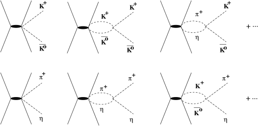
Figure 13: Final state interactions in the coupled channel processes $pp\to dK^{+}\bar{K}^{0}$ and $pp\to d\pi^{+}\eta$. Left panel: Meson–meson FSI that generate the $a_{0}(980)$. Right panel: Meson–baryon FSI sensitive to the $\Lambda(1405)$.

The bubble sum in the coupled $\pi^{+}\eta/\bar{K}^{0}K^{+}$ system generates the $a_{0}(980)$, as described in section 8. On the other hand, the strong $\bar{K}N$ interaction generates the $\Lambda(1405)$, which leaves it trace in the large $\bar{K}d$ scattering length, $a_{\bar{K}d}=(-1.6+i1.9)$ fm. The process at hand is indeed sensitive to the low–energy $\bar{K}N$ amplitude, see the right panel of Fig. 13. Most importantly, these two types of FSI can lead to very strong interference effects, which reveal itself in the invariant mass distributions. Even more dramatic is the prediction for ratio of the total $\pi^{+}\eta$ to the $K^{+}\bar{K}^{0}$ production as a function of the $\theta$ and $\phi$ parameters, see Eq.(10.1). The $\pi^{+}\eta$ production appears mostly around the $a_{0}(980)$ resonance region. In Fig.14 we show the ratio between the integrated $\pi^{+}\eta$ production cross section between $M_{I}=950$ MeV (the invariant mass of the meson pair) and the end of its phase space and the $K^{+}\bar{K}^{0}$ production cross section in all its available phase space. One sees that for most of the values of $\theta$ and $\phi$ the $\pi^{+}\eta$ production rate is substantially larger than that of $K^{+}\bar{K}^{0}$. It is interesting to point out that even in the case when there is no primary $\pi^{+}\eta$ production so that $f^{S}_{\pi\eta}=0$ ($\theta=0$ and any $\phi$ or $\phi=\pi/2$, $3\pi/2$ and any $\theta$), the final state interactions starting from primary $K^{+}\bar{K}^{0}$ production can lead to a $\pi^{+}\eta$ cross section an order of magnitude bigger than that of the $K^{+}\bar{K}^{0}$. One also finds interesting interference effects for some values of $\theta$ and $\phi$ that can reinforce the $\pi^{+}\eta$ production as compared to the $K^{+}\bar{K}^{0}$ as well as other situations when the $K^{+}\bar{K}^{0}$ is produced more copiously than the $\pi^{+}\eta$ channel. The P–wave nature of this reaction can also be seen in the invariant mass distribution of the $\pi^{+}\eta$ system; only after division by the squared three–momentum of the deuteron, the resonance shape of the $a_{0}$ becomes visible. For a more detailed discussion and other interesting predictions, see [98]. Of course much more theoretical effort is needed to achieve a truly systematic and controlled description of these and similar hadronic meson production processes.

Figure 14: $\sigma(\pi^{+}\eta)/\sigma(K^{+}\bar{K}^{0})$ as function of $\theta$ and $\phi$ (in radians).

11 Summary

Let me briefly summarize the salient topics discussed here:

• There are two distinct order parameters characterizing the spontaneous chiral symmetry breaking in QCD, the pion decay constant in the chiral limit, $F$, and the scalar quark condensate, $\Sigma$. The condensate is more sensitive to the IR end of the spectrum of the Euclidean Dirac operator. One expects these order parameters to decrease with increasing number of massless (light) quarks.

• Standard chiral perturbation theory which treats the strange quark as light and is characterized by a large condensate $\Sigma(3)\lesssim\Sigma(2)$ works in many, many instances. OZI violation does not naturally emerge in this scheme, although the OZI suppressed low-energy constants could be large.

• There are some indications that the three–flavor condensate could be sizeably smaller than its two-flavor counterpart, $\Sigma(3)\ll\Sigma(2)$ due to large quantum fluctuations related to light quark loops. In such a scenario, OZI violation would be natural and be related to the sector of the light scalar mesons with vacuum quantum numbers. However, there are still many open questions in this scenario.

• Strange quarks can be treated as heavy matter fields, leading to a reordering of the chiral expansion. Matching conditions relate this heavy kaon scheme to the standard formulation. The heavy kaon approach can e.g. be used to study two–flavor low–energy theorems within SU(3).

• Sigma terms are a direct measure of the QCD quark mass term within hadron states. The sigma terms related to pion–pion and pion–kaon scattering are under control, whereas for the pion–nucleon case the situation is less clear (mostly related to the analysis of $\pi$N scattering data).

• The nature of the low–lying scalar mesons is under debate, although a consistent picture emerges when these are considered as meson–meson resonances due to strong final state interactions. To the contrary, the scalar form factors of the pion and the kaon can be determined to good precision and these can be further applied and tested in many different processes.

• The bound state scenario for some baryons like the $\Lambda(1405)$ can be tested in hadronic and electromagnetic production processes or in transition form factors. Theoretical progress has been made in connecting the coupled channel calculations to chiral perturbation theory.

• Goldstone boson pair production in proton–proton collisions allows for further testing the final state interaction dynamics in the meson–meson and meson–baryon systems. Clearly, the theory of these processes is only in its infancy.

References

- [1] Jamin, M., Oller, J.A. and Pich, A., [arXiv:hep-ph/0110194].
- [2] Ametller, Ll., this volume [arXiv:hep-ph/0112278].
- [3] Bijnens, J., this volume.
- [4] Gasser, J., this volume.
- [5] Holstein, B.R., this volume [arXiv:hep-ph/0112150].
- [6] Banks, T. and Zaks, A., Nucl. Phys. B196, 189 (1982).
- [7] Gardi, E. and Grunberg, G., JHEP 9903, 024 (1999) [arXiv:ep-th/9810192]; Grunberg, G., [arXiv:hep-ph/0009272].
- [8] Sui, C., Nucl. Phys. Proc. Suppl. 73, 228 (1999) [arXiv:hep-lat/9811011]; Mawhinney, R.D., Nucl. Phys. Proc. Suppl. 83, 57 (2000) [arXiv:hep-lat/0001032].
- [9] Iwasaki, Y., Kanaya, K., Kaya, S., Sakai, S. and Yoshié, T., Prog. Theor. Phys. Suppl. 131, 415 (1998) [arXiv:hep-lat/9804005].
- [10] Dalitz, R.H. and Tuan, S.F., Ann. Phys. (NY) 10, 307 (1960).
- [11] Vafa, C. and Witten, E., Nucl. Phys. B234, 173 (1984).
- [12] Weinberg, S., Physica 96A, 327 (1979).
- [13] Gasser, J. and Leutwyler, H., Ann. Phys. (NY) 158, 142 (1984).
- [14] J. Gasser and H. Leutwyler, Nucl. Phys. B250, 465 (1985).
- [15] Banks, T. and Casher, A., Nucl. Phys. B169, 103 (1980).
- [16] Leutwyler, H. and Smilga, A., Phys. Rev. D46, 5632 (1992).
- [17] Stern, J., [arXiv:hep-ph/9801282].
- [18] Descotes, S., Girlanda, L. and Stern, J., JHEP 0001, 041 (2000) [arXiv:hep-ph/0010537].
- [19] Duncan, A., Eichten, E. and Thacker, H., Phys. Rev. D59, 014505 (1999) [arXiv:hep-lat/9806020].
- [20] Pislak, S. et al. (BNL-E865 Collaboration), Phys. Rev. Lett. 87, 221801 (2001) [arXiv:hep-ex/0106071].
- [21] Witten, E., Nucl. Phys. B160, 57 (1979).
- [22] Meißner, Ulf-G. and Oller, J.A., Nucl. Phys. A679, 671 (2001) [arXiv:hep-ph/0005253].
- [23] Moussallam, B., Eur. Phys. J. C14, 111 (2000) [arXiv:hep-ph/9909292].
- [24] Moussallam, B., JHEP 0008, 005 (2000) [arXiv:hep-ph/0005245].
- [25] Descotes, S., “Effet des boucles de quarks légers sur la structure de vide de QCD”, Thèse de doctorat, Université Paris-XI, Orsay, France (2000).
- [26] Descotes, S. and Stern, J., Phys. Lett. B488, 274 (2000) [arXiv:hep-ph/0007082].
- [27] Oller, J.A., Oset, E. and Pelaez, J.R., Phys. Rev. D59, 074001 (1999) [arXiv:hep-ph/9804029].
- [28] Au, K.L., Morgan, D. and Pennington, M.R., Phys. Rev. D35, 1633 (1987).
- [29] Kaminsky, R., Lesniak, L. and Maillet, J.P., Phys. Rev. D50, 3145 (1994) [arXiv:hep-ph/9403264]; Kaminsky, R., Lesniak, L. and Loiseau, B., Phys. Lett. B413, 130 (1997) [arXiv:hep-ph/9707377].
- [30] Descotes, S., JHEP 0103, 002 (2001) [arXiv:hep-ph/0012221].
- [31] Descotes, S. and Stern, J., Phys. Rev. D62, 054011 (2000) [arXiv:hep-ph/9912234].
- [32] Amoros, G., Bijnens, J., and Talavera, P., Nucl. Phys. B585, 293 (2000); Erratum ibid B598, 665 (2001) [arXiv:hep-ph/0003258].
- [33] Bijnens, J., Ecker, G. and Gasser, J., in The second DAPHNE physics handbook, Maiani, L., Pancheri, G. and Paver, N. (editors), INFN Frascati, 1995 [arXiv:hep-ph/9411232].
- [34] Bernard, V., Kaiser, N. and Meißner, Ulf-G., Nucl. Phys. B357, 129 (1991); Phys. Rev. D43, R2757 (1991).
- [35] Johannesson, N.O. and Nilsson, G., Nuovo Cimento 43A, 376 (1978).
- [36] Kubis, B. and Meißner, Ulf-G., Phys. Lett. B (2002) in print [arXiv:hep-ph/0112154].
- [37] Ananthanarayan, B. and Büttiker, P., Eur. Phys. J. C19, 517 (2001) [arXiv:hep-ph/0012023].
- [38] Bernard, V., Kaiser, N. and Meißner, Ulf-G., Phys. Rev. C52, 2185 (1995).
- [39] Ananthanarayan, B., Büttiker, P. and Moussallam, B., Eur. Phys. J. C22, 133 (2001) [arXiv:hep-ph/0106230].
- [40] Jamin, M., Oller, J.A. and Pich, A., Nucl. Phys. B587, 331 (2000) [arXiv:hep-ph/0006045].
- [41] Bernard, V., Kaiser, N. and Meißner, Ulf-G., Nucl. Phys. B364, 283 (1991).
- [42] Adeva, B. et al., CERN/SPSC 2000-032.
- [43] Kubis, B. and Meißner, Ulf-G., Nucl. Phys. A699, 709 (2002) [arXiv:hep-ph/0107199].
- [44] Nehme, A. and Talavera, P., [arXiv:hep-ph/0107299].
- [45] Nehme, A., [arXiv:hep-ph/0111212].
- [46] Callan, C.G. Jr. and Klebanov, I.R., Nucl. Phys. B262, 365 (1985).
- [47] A. Roessl, Nucl. Phys. B555, 507 (1999) [arXiv:hep-ph/9904230].
- [48] S.M. Ouellette, [arXiv:hep-ph/0101055].
- [49] Jenkins, E. and Manohar, A.V., Phys. Lett. B255, 558 (1991).
- [50] Bernard, V., Kaiser, N. and Meißner, Ulf-G., Int. J. Mod. Phys. E4, 193 (1995). [arXiv:hep-ph/9501384].
- [51] Lang, C.B., Fortschr. Phys. 26, 509 (1978).
- [52] Frink, M., Kubis, B. and Meißner, Ulf-G., in preparation.
- [53] Brown, L.S., Pardee, W.J. and Peccei, R.D., Phys. Rev. D4, 2801 (1971)
- [54] Cheng, T.P. and Dashen, R., Phys. Rev. Lett. 26, 594 (1971).
- [55] Gasser, J. and Sainio, M.E., in Physcis and Detectors for DANE, Frascati Physics Series Vol. 16, S. Bianco et al. (eds) (Frascati, 1999) [arXiv:hep-ph/0002283].
- [56] Bernard, V., Kaiser, N. and Meißner, Ulf-G., Phys. Lett. B389, 144 (1999) [arXiv:hep-ph/9607245].
- [57] Gasser, J., Ann. Phys. (NY) Ann. Phys. (NY) 136, 62 (1981).
- [58] Borasoy, B. and Meißner, Ulf-G., Ann. Phys. 254, 192 (1997) [arXiv:hep-ph/9607432].
- [59] Fettes, N. and Meißner, Ulf-G., Nucl. Phys. A693, 693 (2001) [arXiv:hep-ph/0101030].
- [60] Fettes, N. and Meißner, Ulf-G., Nucl. Phys. A676, 311 (2000) [arXiv:hep-ph/0002162].
- [61] Büttiker, P. and Meißner, Ulf-G., Nucl. Phys. A668, 97 (2000) [arXiv:hep-ph/9908247].
- [62] Becher, T. and Leutwyler, H., Eur. Phys. J. C9, 643 (1999) [arXiv:hep-ph/9901384].
- [63] Becher, T. and Leutwyler, H., JHEP 0106, 017 (2001) [arXiv:hep-ph/0103263].
- [64] Gasser, J., Leutwyler, H. and Sainio, M.E., Phys. Lett. B253, 252 (1991); ibid 260.
- [65] Meißner, Ulf-G. and Smith, G., [arXiv:hep-ph/0011277].
- [66] Pavan, M.M., Arndt, R.A., Strakovsky, I.I. and Workman, R.L., [arXiv:hep-ph/0111066].
- [67] Pennington, M.R., Physcis and Detectors for DANE, Frascati Physics Series Vol. 16, S. Bianco et al. (eds) (Frascati, 1999) [arXiv:hep-ph/9905241].
- [68] Meißner, Ulf-G., Comm. Nucl. Part. Phys. 20 (1991) 119.
- [69] Geiger, P. and Isgur, N., Phys. Rev. D47, 5050 (1993).
- [70] Oller, J.A. and Oset, E., Nucl. Phys. A620, 438 (1997); (E) Nucl. Phys. A652, 407(1999) [arXiv:hep-ph/9702314].
- [71] Oller, J.A. and Oset, E., Phys. Rev. D60, 074023 (1999) [arXiv:hep-ph/9809337].
- [72] Morgan, D. and Pennington, M.R., Phys. Rev. D48, 1185, 5422 (1993).
- [73] Oller, J.A. and Oset, E., Nucl. Phys. A629, 739 (1998) [arXiv:hep-ph/9706487].
- [74] Marco, E., Hirenzaki, S., Oset, E. and Toki, H., Phys. Lett. B470, 20 (1999) [arXiv:hep-ph/9903217].
- [75] Achasov, M.N. et al., Phys. Lett. B440, 442 (1998).
- [76] Achasov, N.N. and Ivanchenko, V.N. Nucl. Phys. B315, 465 (1989); Achasov, N.N., Gubin, V.V. and Solodov, E.P., Phys. Rev. D55, 2672 (1997).
- [77] Falvard, A. et al., Phys. Rev. D38, 2706 (1988).
- [78] Lockman, W.S., “Production of the Meson in the Decays”, Ajaccio Hadron 1989, page 109.
- [79] Donoghue, J.F., Gasser, J. and Leutwyler, H., Nucl. Phys. B343, 341 (1990).
- [80] Aitala, M. et al. [E791 Collaboration], Phys. Rev. Lett. 86, 770 (2001) [arXiv:hep-ex/0007028].
- [81] Gardner, S. and Meißner, Ulf-G., [arXiv:hep-ph/0112281].
- [82] Deandrea, A. and Polosa, A.D., Phys. Rev. Lett. 86, 216 (2001) [arXiv:hep-ph/0008084].
- [83] Kaiser, N., Siegel, P.B. and Weise, W., Nucl. Phys. A594, 325 (1995) [arXiv:nucl-th/9505043].
- [84] Oset, E. and Ramos, A., Nucl. Phys. A635, 99 (1998) [arXiv:nucl-th/9711022].
- [85] Meißner, Ulf-G. and Oller, J.A., Nucl. Phys. A673, 311 (2000) [arXiv:nucl-th/9912026].
- [86] Meißner, Ulf-G. and Oller, J.A., Phys. Lett. B500, 263 (2001) [arXiv:hep-ph/0011146].
- [87] G. Höhler, in Landolt-Börnstein, Vol. 9b2, H. Schopper (ed.), Springer Verlag, Berlin (1983); Hanstein, O., Drechsel, D. and Tiator, L., Phys. Lett. B385, 45 (1996) [arXiv:nucl-th/9605008].
- [88] Kaiser, N., Siegel, P.B. and Weise, W., Phys. Lett. B362, 23 (1995) [arXiv:nucl-th/9507036].
- [89] Oset, E., Ramos, A., and Bennhold, C., Phys. Lett. B, in print [arXiv:nucl-th/0109006].
- [90] Nacher, J.C., Oset, E., Toki, H. and Ramos, A., Phys. Lett. B455, 55 (1999). [arXiv:nucl-th/9812055].
- [91] Frankfurt, L., Johnson, M., Sargsian, M., Weise, W. and Strikman, M., Phys. Rev. C60, 055202 (1999) [arXiv:nucl-th/9808016].
- [92] Kilian, K., Meißner, Ulf-G. and Speth, J., Phys. Bl. 54, 911 (1998).
- [93] Machner, H. and Haidenbauer, J., J. Phys. G25, R231 (1991); Nakayama, K., [arXiv:nucl-th:0108032]; Gronzka, D. and Kilian, K., Nucl. Phys. A684, 130c (2001); Kühn, W. et al., Nucl. Phys. A684, 440c (2001); Fäldt, G. and Wilkin, C., Phys.Scripta 64, 427 (2001) [arXiv:nucl-th/0104081].
- [94] Fäldt, G., Johansson, T. and Wilkin, C., this volume.
- [95] Barsov, S. et al., Nucl. Instrum. Meth. A462, 364 (2001).
- [96] Grishina, V.Yu., Kondratyuk, L.A., Bratkovskaya, E.L., Büscher, M. and Cassing, W., Eur. Phys. J. A9, 277 (2000) [arXiv:nucl-th/0007074]; Bratkovskaya, E.L., Grishina, V.Yu., Kondratyuk, L.A., Büscher, M. and Cassing, W., [arXiv: nucl-th/0107071].
- [97] Bernard, V., Kaiser, N. and Meißner, Ulf-G., Phys. Rev. D44, 3698 (1991); Ecker, G., Gasser, J., Pich, A. and de Rafael, E., Nucl. Phys. B321, 311 (1989).
- [98] Oset, E., Oller, J.A. and Meißner, Ulf-G., Eur. Phys. J. A (2002), in print [arXiv: nucl-th/0109050].