Can Van Hove singularities be observed in relativistic heavy-ion collisions ?

Abstract

Based on general arguments the in-medium quark propagator in a quark-gluon plasma leads to a quark dispersion relation consisting of two branches, of which one exhibits a minimum at some finite momentum. This results in a vanishing group velocity for collective quark modes. Important quantities such as the production rate of low mass lepton pairs and mesonic correlators depend inversely on this group velocity. Therefore these quantities, which follow from self energy diagrams containing a quark loop, are strongly affected by Van Hove singularities (peaks and gaps). If these sharp structures could be observed in relativistic heavy-ion collisions it would reveal the physical picture of the QGP as a gas of quasiparticles.

1. Introduction

Recently, Van Hove singularities in the QGP  [?,?,?,?,?,?], caused by the collective quark modes appearing due to the interaction with the medium, have attracted great attention as they could probe the QGP as a gas of quasiparticles formed in heavy-ion collisions. One of the quark modes, the plasmino branch, has a minimum at some finite momentum leading to a vanishing group velocity. Thus the density of states, which is inversely proportional to the group velocity, diverges, causing Van Hove singularities on relevant quantities like the dilepton production rate and mesonic correlators. Here we would like to discuss the role of Van Hove singularities in the QGP.

In the next section, we briefly recall the classic idea of Van Hove singularities in the density of states as discussed in the context of condensed matter physics. We will demonstrate in the following two sections that Van Hove singularities appear as a dynamical aspect of QGP on account of the effective quark propagator containing the quark self-energy. In sec.3 we will demonstrate this through the hadronic correlators using the hard thermal loop (HTL) resummed qurak propagator whereas in sec. 4 through the nonperturbative dilepton production rate, using an effective quark propagator obtained by taking into account the nonperturbative gluon condensate above the critical temperature derived from lattice QCD. In sec. 5 we will argue that the minimum in the plasmino branch and thus the appearance of Van Hove singularities is a general property of massless fermions at finite temperature. Finally, in sec. 6 we will discuss the possibilities and difficulties to observe Van Hove singularities which could reflect the physical picture of the QGP as a gas of quasiparticles produced in heavy-ion collisions.

2. Van Hove Singularities

In condensed matter physics Van Hove singularities in the density of states were discussed on structural aspects of a solid by Van Hove  [?] in 1953. The density of state of a system (e.g. phonons, electrons) is given as

$$g(\omega)=\sum_{n}\int\frac{{\rm d}^{3}k}{(2\pi)^{3}}\>\delta(\omega-\omega_{n}(\mbox{\boldmath$k$})),$$ (1)

implying the number of allowed wave vectors $k$ in the level $n$ having energy $\omega_{n}(\mbox{\boldmath$k$})$ within the energy interval $\omega$ and $\omega+{\rm d}\omega$. By surface integration it can be given  [?] as

$$g(\omega)=\sum_{n}\int\frac{{\rm d}S_{\omega}}{(2\pi)^{3}}\>\frac{1}{|{\bf\nabla}\omega_{n}(\mbox{\boldmath$k$})|},$$ (2)

which is explicitly related to the group velocity, ${|{\bf\nabla}\omega_{n}(\mbox{\boldmath$k$})|}$, which is the derivative of the dispersion relation. Due to symmetries in a crystal the group velocity vanishes at certain momenta, resulting in a divergent integrand in (2). This divergence is integrable in 3-dimensions, leading to a finite density of states. In lower dimensions, however, Van Hove singularities appear. For example, a 2-dimensional electron gas shows logarithmic singularities, which have been discussed in connection with high-$T_{c}$ superconductors  [?]. A 2-dimensional electron gas has also been discussed widely in the context of the quantum Hall effect. As discussed here, the Van Hove singularities are linked to the structural aspect of a solid whereas, as we will see below, in the QGP they are due to dynamical reasons.

3. Thermal Hadronic Correlaton Function

3.1 Definition

Meson correlators are constructed from meson currents $J_{M}(\tau,\vec{x})=\bar{q}(\tau,\vec{x})\Gamma_{M}q(\tau,\vec{x})$, where $\Gamma_{M}=1$, $\gamma_{5}$, $\gamma_{\mu}$, $\gamma_{\mu}\gamma_{5}$ for scalar, pseudo-scalar, vector and pseudo-vector channels, respectively. The thermal two-point functions in coordinate space, $G_{M}(\tau,\vec{x})$, are defined as

$$G_{M}(\tau,\vec{x}) = \langle J_{M}(\tau,\vec{x})J_{M}^{\dagger}(0,\vec{0})\rangle$$ (3)

$$= T\sum_{n=-\infty}^{\infty}\int{{\rm d}^{3}p\over(2\pi)^{3}}\;{\rm e}^{-i(\omega_{n}\tau-\vec{p}\vec{x})}\;\chi_{M}(\omega_{n},\vec{p})~{}~{},$$ (4)

where $\tau\in[0,1/T]$, and the Fourier transformed correlation function $\chi_{M}(\omega_{n},\vec{p})$ is given at the discrete Matsubara modes, $\omega_{n}=2n\pi T$. The imaginary part of the momentum space correlator gives the spectral function $\sigma_{M}(\omega,\vec{p})$,

$$\chi_{M}(\omega_{n},\vec{p})=-\int_{-\infty}^{\infty}{\rm d}\omega{\sigma_{M}(\omega,\vec{p})\over i\omega_{n}-\omega+i\epsilon}\Rightarrow\sigma_{M}(\omega,\vec{p})={1\over\pi}{\rm Im}\;\chi_{M}(\omega,\vec{p}).$$ (5)

Using eqs. (4) and (5) we obtain the spectral representation of the thermal correlation function in coordinate space at fixed momentum ($\beta=1/T$),

$$G_{M}(\tau,\vec{p})=\int_{0}^{\infty}{\rm d}\omega\;\sigma_{M}(\omega,\vec{p})\;{{\rm cosh}(\omega(\tau-\beta/2))\over{\rm sinh}(\omega\beta/2)}~{}~{}.$$ (6)

3.2 Hard Thermal Loop (HTL) Approximation

Perturbative QCD at finite temperature is based on the fact that the temperature dependent running coupling constant is small at high temperatures due to asymptotic freedom, $T\rightarrow\infty\Rightarrow\alpha_{s}(T)=g^{2}/4\pi\rightarrow 0$. At a typical temperature of $T=250$ MeV we expect $\alpha_{s}=0.3$ – 0.5. This suggests that perturbative theory could work at least qualitatively.

However, restricting only to bare propagators and vertices perturbative QCD can lead to serious problems, i.e., infrared divergent and gauge dependent results for physical quantities, e.g., in the case of the damping rate of a long wave, collective gluon mode in the QGP. The sign and magnitude of the gluon damping rate was found to be strongly gauge dependent  [?,?]. The reason for such behaviour is the fact that bare perturbative QCD at finite temperature is incomplete, i.e., higher order diagrams missing in bare perturbation theory can contribute to lower order in coupling constant. In order to overcome these problems, the HTL resummation technique, an improved perturbation theory, has been suggested by Braaten and Pisarski  [?] and also by Frenkel and Taylor  [?], in which those diagrams can be taken into account by resummation. The following prescription has been suggested for the improved perturbation theory:

1. Isolate those diagrams which should be resummed. The starting point is the separation of scales in the weak coupling limit, $g<<1$, since there are two momentum scales in a plasma of massless particles: (i) hard, where the momentum $\sim$ temperature, $T$ and (ii) soft, where the momentum $\sim$ thermal mass ($\sim\ gT$, $g<<1$). These diagrams are HTL self energies and vertices given by one loop diagram, where the external momenta are soft and the loop momenta are hard. For example, in the case of self energies in QED or QCD a result proportional to $g^{2}T^{2}$ was obtained, which is equivalent to the high temperature approximation, $T>>p,\ \ |p_{0}|$, found earlier by Klimov   [?] and Weldon  [?], and also to the semiclassical approximation by Silin  [?].

2. Effective propagators in the HTL approximation are constructed using the Dyson-Schwinger equations. The HTL vertex follows simply by adding the HTL correction to the bare vertex. This effective vertex is also related, except for scalar particles, to the HTL propagator through Ward identity.

3. These effective quantities, propagators and vertices, can then be used as in ordinary perturbation theory if all legs are soft, leading to results that are complete to leading order in the coupling constant, gauge independent and improved in the infrared behaviour. If, on the other hand, at least one leg of the propagtors or vertices is hard, bare quantities are sufficient.

3.3 Quark self energy in HTL-approximation

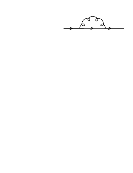
Figure  1.: Quark self energy having quark momentum $K$.

The most general ansatz for the fermionic self energy in rest frame of the plasma is given by  [?]

$$\Sigma(K)=-a(k_{0},k)K\!\!\!\!/\,-b(k_{0},k)\gamma_{0}\ ,$$ (7)

where $K=(k_{0},{\bf k})$, $k=|{\bf k}|$ and the quark mass is neglected assuming that the temperature is much larger than the quark mass, which holds at least for $u$ and $d$ quarks. The scalar quantities $a$ and $b$ are given by the traces over self energies in figure 1 as, respectively,

$$a(k_{0},k) = \frac{1}{4k^{2}}\>\left[{\rm{tr}}\,(K\!\!\!\!/\,\Sigma)-k_{0}\>{\rm{tr}}\,(\gamma_{0}\Sigma)\right],$$ (8)

$$b(k_{0},k) = \frac{1}{4k^{2}}\>\left[K^{2}\>{\rm{tr}}\,(\gamma_{0}\Sigma)-k_{0}\>{\rm{tr}}\,(K\!\!\!\!/\,\Sigma)\right],$$ (9)

and obtained in HTL-approximation as

$$a(k_{0},k) = \frac{m_{q}^{2}}{k^{2}}\>\left(1-\frac{k_{0}}{2k}\>\ln\frac{k_{0}+k}{k_{0}-k}\right)\ \ ,$$ (10)

$$b(k_{0},k) = \frac{m_{q}^{2}}{k^{2}}\>\left(-k_{0}+\frac{k_{0}^{2}-k^{2}}{2k}\>\ln\frac{k_{0}+k}{k_{0}-k}\right)\ \ ,$$ (11)

where $m_{q}^{2}={g^{2}T^{2}}/{6}$, is the effective quark mass. The quark self energy in eq.(7) has an imaginary part below the light cone, $k_{0}^{2}-k^{2}<0$, representing Landau damping for space like quark momenta. Furthermore, the general ansatz in eq.(7) is also chirally invariant in spite of the appearance of an effective quark mass.

3.4 Effective Propagators and Vertices in HTL-approximation

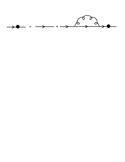
Figure  2.: Effective quark propagator in HTL-approximation

Resumming the quark self-energy by using the Dyson-Schwinger equation, the effective quark propagator in figure 2 can be written as

$$S(K)=[K\!\!\!\!/\,-\Sigma(K)]^{-1}.$$ (12)

For massless quarks, decomposing the effective quark propagator in (12) into helicity eigenstates, we get

$$S(K)=\frac{\gamma_{0}-\hat{\bf k}\cdot{\vec{\gamma}}}{2D_{+}(K)}+\frac{\gamma_{0}+\hat{\bf k}\cdot{\vec{\gamma}}}{2D_{-}(K)}\ \ ,$$ (13)

with

$$D_{\pm}(k_{0},k)=(1+a(k_{0},k))\>(-k_{0}\pm k)+b(k_{0},k)\ \ \ .$$ (14)

The relevant QED like HTL-vertex is related to this propagator through the Ward identity  [?,?]

$$K_{\mu}\Gamma^{\mu}(K_{1},K_{2};K)=S^{-1}(K_{1})-S^{-1}(K_{2})\ \ .$$ (15)

Figure  3.: Quark dispersion relation in HTL-approximation along with the free ($\omega=k$) one.

Now, the zeros of $D_{\pm}(K)$ give the in-medium dispersion relation for quarks. As shown in figure 3 the upper curve $\omega_{+}(k)$ corresponds to the solution of $D_{+}(K)=0$, whereas the lower curve $\omega_{-}(k)$ represents the solution of $D_{-}(K)=0$. Both branches start from a common effective mass, $m_{q}$, obtained in the $k\rightarrow 0$ limit  [?]. The $\omega_{+}(k)$ branch describes the propagation of an ordinary quark with thermal mass, and the ratio of its chirality to helicity is $+1$. On the other hand, the $\omega_{-}(k)$ branch corresponds to the propagation of a quark mode with a negative chirality to helicity ratio. This branch represents the plasmino mode which is absent in the vacuum but appears as consequence of the medium due to the broken Lorentz invariance, and has a shallow minimum. This corresponds to a purely collective long wave-length mode, whose spectral strength decreases exponentially at high momenta. For high momenta, however, both branches approach the free dispersion relation.

3.5 Hadronic spectral and correlation function in HTL-approximation

The hadronic spectral functions, $\sigma_{M}(\omega,p)$ in (5), of the temporal correlators are proportional to the imaginary part of the quark loop diagram. Here we will calculate the imaginary part of the quark loop diagram corresponding to the vector meson channel, which is related to the static dilepton production rate (${\vec{p}}=0$) as  [?]

$$\sigma_{V}(\omega)=\frac{1}{\pi}{\rm{Im}}\ \chi_{V}(\omega)=\frac{18\pi^{2}N_{C}}{5\alpha^{2}}\left(e^{\beta\omega}-1\right)\omega^{2}\frac{dR}{d^{4}xd\omega d^{3}p}({\vec{p}}=0).$$ (16)

For the details of the other channels, e.g., pseudovector, scalar and pseudoscalar, see Refs.  [?,?].

Figure  4.: Self-energy diagram involving quarks loop in HTL-approximation.

Now the vector meson correlation function can be written from figure 4 as

$$\chi_{V}\left(\omega,p\right)=2N_{C}T\sum_{k_{0}}\int\frac{d^{3}k}{(2\pi)^{3}}{\rm{tr}}\left[S\left(K\right)\Gamma^{\mu}(-Q,-K;P)S\left(Q\right)\Gamma^{\nu}(Q,K;-P)\right]\,,$$ (17)

where, $Q=P-K$, $N_{C}=3$ and $\chi_{V}$ denotes the trace over the Lorentz indices of $\chi_{M}^{\mu\nu}$. Using the effective quantities from (13) and (15), eq. (16) at ${\vec{p}}=0$ can be written as

$$\sigma_{V}(\omega) = \frac{4N_{c}}{{\pi^{2}}}(e^{\beta\omega}-1)\int^{\infty}_{0}dk\,k^{2}\int_{-\infty}^{+\infty}dx\int^{+\infty}_{-\infty}dx^{\prime}n_{F}\left(x\right)n_{F}\left(x^{\prime}\right)\delta\left(\omega-x-x^{\prime}\right)$$ (21)

$$\times\left\{4\left(1-\frac{x^{2}-x^{\prime 2}}{2k\omega}\right)^{2}\rho_{+}\left(x,k\right)\rho_{-}\left(x^{\prime},k\right)+\left(1+\frac{x^{2}+x^{\prime 2}-2k^{2}-2m_{q}^{2}}{2k\omega}\right)^{2}\right.$$

$$\left.\times\rho_{+}\left(x,k\right)\rho_{+}\left(x^{\prime},k\right)+\left(1-\frac{x^{2}+x^{\prime 2}-2k^{2}-2m_{q}^{2}}{2k\omega}\right)^{2}\rho_{-}\left(x,k\right)\rho_{-}(x^{\prime},k)\right.$$

$$\left.+\theta\left(k^{2}-x^{2}\right)\frac{m^{2}_{q}}{4k\omega^{2}}\left(1-\frac{x^{2}}{k^{2}}\right)\left[\left(1+\frac{x}{k}\right)\rho_{+}\left(x^{\prime},k\right)+\left(1-\frac{x}{k}\right)\rho_{-}\left(x^{\prime},k\right)\right]\ \right\},$$

where $x$ and $x^{\prime}$ are the energies of the internal particles, $n_{F}$ is the fermi distribution function, and $\rho_{\pm}$ are the spectral function for collective quark modes in the medium  [?] having a pole contribution from the in-medium dispersion relation and a cut contribution for space like quark momenta related to Landau damping below the light cone ($k_{0}^{2}<k^{2}$). The meson spectral function, constructed from two quark propagators, will have pole-pole, pole-cut and cut-cut contributions, $\sigma_{M}(\omega)=\sigma^{\rm{pp}}(\omega)+\sigma^{\rm{pc}}(\omega)+\sigma^{\rm{cc}}(\omega)$. Here we quote only the pole-pole expression for vector mesons,

$$\sigma_{V}^{\rm{pp}} = \frac{1}{4m^{4}_{q}}\left[{k^{2}_{1}}n^{2}_{F}\left(\omega_{+}\left(k_{1}\right)\right)\frac{\left(\omega^{2}_{+}\left(k_{1}\right)-k^{2}_{1}\right)^{2}}{2\omega_{+}^{\prime}(k_{1})}\left(1+\frac{\omega^{2}_{+}\left(k_{1}\right)-k^{2}_{1}-m^{2}_{q}}{k_{1}\omega}\right)^{2}\right.$$ (22)

$$+ \left.k^{2}_{2}n\,^{2}_{F}\left(\omega_{-}\left(k_{2}\right)\right)\left(1-\frac{\omega^{2}_{-}\left(k_{2}\right)-k^{2}_{2}-m^{2}_{q}}{k_{2}\omega}\right)^{2}\frac{\left(\omega^{2}_{-}\left(k_{2}\right)-k^{2}_{2}\right)^{2}}{2\omega_{-}^{\prime}(k_{2})}\right.$$ (23)

$$+ \left.2k^{2}_{3}\,n_{F}\left(\omega_{+}\left(k_{3}\right)\right)n_{F}\left(-\omega_{-}\left(k_{3}\right)\right)\frac{\left(\omega^{2}_{+}\left(k_{3}\right)-k^{2}_{3}\right)\left(\omega^{2}_{-}\left(k_{3}\right)-k^{2}_{3}\right)}{\omega_{+}^{\prime}(k_{3})-\omega_{-}^{\prime}(k_{3})}\right.$$ (24)

$$\times \left.\left(1+\frac{\omega^{2}_{+}\left(k_{3}\right)+\omega^{2}_{-}\left(k_{3}\right)-2k^{2}_{3}-2m^{2}_{q}}{2k_{3}\omega}\right)^{2}\right]\ ,$$ (25)

where $k_{1}$ is the solution of $\omega-2\omega_{+}(k)=0$, and $k_{2}^{i}$ and $k_{3}^{i}$ are the solutions of $\omega-2\omega_{-}(k)=0$ and $\omega-\omega_{+}(k)+\omega_{-}(k)=0$, respectively, which can have two solutions at low momenta due to the plasmino mode. Each term in (25) corresponds to different physical processes  [?,?,?] and is inversely proportional to the derivative of the dispersion relation (group velocity). The other contributions ($\sigma^{\rm{pc}}$ and $\sigma^{\rm{cc}}$) can easily be obtained  [?,?,?] from (21). Similar results for the scalar channel have also been derived and detailed discussions are given in Ref.  [?,?]. Free meson spectral functions are also obtained using bare propagators and vertices in figure 4 as  [?,?]

$$\sigma^{{\rm free}}_{M}\left(\omega\right)=\frac{N_{C}}{4\pi^{2}}\omega^{2}\tanh\left(\frac{\omega}{4T}\right)a_{M}\ \ ,$$ (26)

where $a_{M}=(+)-1$ for (pseudo)scalar and $(-)+2$ for (pseudo)vector.

Figure  5.: (a) Pseudoscalar and (b) vector meson spectral functions in HTL approximation for $m_{q}/T=1$. The free one is represented by crosses.

In figure 5 we show the different contributions for pseudoscalar and vector mesons for $m_{q}/T=1$, i.e., $g=\sqrt{6}$. Generically the pole-pole term of the meson spectral function in HTL-approximation describes three physical processes: (1) the annihilation of collective quarks (e.g., 1^st term in (25)), (2) the annihilation of two plasminos (2^nd term in (25)) and (3) the transition from upper to lower branch (3^rd term in (25)). The transition process starts at zero energy and continues until the maximum difference $\omega=0.47\>m_{q}$ between the two branches at $k_{3}=1.18\>m_{q}$. At this point a Van Hove singularity is encountered due to the vanishing denominator $\omega^{\prime}_{+}(k_{3})-\omega^{\prime}_{-}(k_{3})=0$, implying a diverging density of states. The plasmino annihilation starts at $\omega=1.86\>m_{q}$ with another Van Hove singularity corresponding to the minimum of the plasmino branch at $k_{3}=0.41\>m_{q}$, where $\omega^{\prime}_{-}(k_{2})=0$. This contribution falls off rapidly due to the exponentially suppressed spectral strength of the plasmino mode for large energies, where only the first process, quark-antiquark annihilation starting at $\omega=2m_{q}$, contributes. For large energies this dominates and approaches the free results (crosses) for $\omega>>m_{q}$. The pole-cut and cut-cut contributions, which involve external gluons as can be seen by cutting the HTL quark self energy, lead to a smooth contribution to the spectral function. The pole-pole and pole-cut contributions in both channels are of similar magnitude, while the cut-cut contribution at small $\omega$ vanishes in the pseudoscalar channel but diverges in the vector channel. This has its origin in the structure of HTL quark-meson vertex  [?,?], which is required for the vector channel containing a collinear singularity  [?], whereas bare vertices are sufficient for the (pseudo)scalar channel. This implies that higher order diagrams in the HTL expansion contribute to the same order in the coupling constant  [?], which, of course, indicates that the low frequency part of the vector meson spectral function is inherently nonperturbative. As discussed, the vector meson spectral function is linked to the dilepton production  [?,?] at high temperature whereas the pseudoscalar correlator is related to the chiral condensate and thus to the chiral susceptibility  [?,?].

Figure  6.: The subtracted thermal pseudoscalar (left) and vector (right) meson correlation functions in HTL-approximation for $m_{q}/T=2$.

The temporal correlators for pseudoscalar and vector mesons can be obtained from their spectral function according to (6). The competing effects of pole and cut contributions in the spectral function carries over to the correlation functions, which is found to be almost similar  [?,?], unlike in lattice calculations  [?], to the free one with bare propagators and vertices. A linear divergence, due to the effective HTL-vertices, of the spectral function in the vector channel at low frequencies also renders the temporal correlator infrared divergent. Although the pseudoscalar correlation functions are infrared finite, the low frequency part of the spectral functions will also be modified significantly from contributions of higher order diagrams. It is reasonable to consider modified correlation functions, $\Delta{G}_{M}(\tau)\equiv{G}_{M}(\tau)-{G}_{M}(\beta/2)$, which are less sensitive to details of the low frequency part of the spectral functions. In the subtracted correlation functions the infrared divergences are eliminated. As shown in figure 6 they are well-defined in both channels. One observes that after elimination of the infrared divergent parts the structure of the pole and cut contributions is similar in the scalar and vector channel. The vector correlator seems to be even closer to the leading order perturbative (free) correlator than the scalar one.

4. Gluon condensate and nonperturbative dilepton production

It seems that quite generally nonperturbative effects  [?] dominate the temperature regime attainable in heavy-ion collisions and the application of perturbative calculations there becomes questionable as the coupling constant is not small. Such nonperturbative effects were made explicit by lattice QCD calculations  [?] below and above the phase transition temperature. The gluon condensate, which appears due to the broken scale invariance at zero as well as at finite temperature, describes the nonperturbative imprints of the QCD ground states and have extensively been used for studying hadron properties at zero and finite temperature. Lattice QCD so far is not capable to compute dynamical quantities. As an alternative method to lattice and perturbative QCD it has been suggested to include the gluon condensate obtained from lattice QCD into the parton propagators at zero  [?] as well at finite  [?] temperature. In this way, nonperturbative effects are taken into account within the Green functions technique, which then can be exploited to calculate various physical quantities like the dilepton rate, hadronic correlators, susceptibilities, etc.

4.1 Quark propagation

Figure  7.: Quark self-energy diagram in the presence of the gluon condensate.

Now, the functions $a(k_{0},k)$ and $b(k_{0},k)$ in the general effective quark propagator at finite temperature defined in (13) and (14) can be obtained using self energy diagram with the gluon condensate in figure 7 as  [?,?,?]

$$a = -\frac{g^{2}}{6}\frac{1}{K^{6}}\biggl{[}\left(\frac{1}{3}k^{2}-\frac{5}{3}k_{0}^{2}\right)\langle{\mathcal{E}}^{2}\rangle_{T}-\left(\frac{1}{5}k^{2}-k_{0}^{2}\right)\langle{\mathcal{B}}^{2}\rangle_{T}\biggr{]},$$ (27)

$$b = -\frac{4}{9}g^{2}\frac{k_{0}}{K^{6}}\left[k_{0}^{2}\langle{\mathcal{E}}^{2}\rangle_{T}+\frac{1}{5}k^{2}\langle{\mathcal{B}}^{2}\rangle_{T}\right],$$ (28)

with the chromoelectric and and chromomagnetic condensates expressed  [?,?,?] in terms of the space like ($\Delta_{\sigma}$) and time like ($\Delta_{\tau}$) plaquette expectation values as

$$\frac{\alpha_{s}}{\pi}\langle{\cal E}^{2}\rangle_{T} = \frac{4}{11}T^{4}\Delta_{\tau}-\frac{2}{11}\langle G^{2}\rangle_{T=0}\ ,$$ (29)

$$\frac{\alpha_{s}}{\pi}\langle{\cal B}^{2}\rangle_{T} = -\frac{4}{11}T^{4}\Delta_{\sigma}+\frac{2}{11}\langle G^{2}\rangle_{T=0}\ ,$$ (30)

where $\langle G^{2}\rangle_{T=0}=(2.5\pm 1.0)T_{c}^{4}$ and the plaqutte values are taken from lattice calculations  [?]. This propagator is also related to an effective vertex  [?] through the QED like Ward identity. The dispersion relation in the presence of the gluon condensate is shown in figure 8, which shows the same qualitative features as in the HTL case (figure 3) although it is a completely different approximation. However, the thermal mass of the quark is $m_{\rm{eff}}\sim 1.15T$, which is independent of the coupling constant unlike in the HTL case.

Figure  8.: Quark dispersion relation in the presence of the gluon condensate with $T=1.1T_{c}$ (left) and $T=4T_{c}$ (right). Here, read l=$k$.

4.2 Nonperturbative dilepton production

Figure  9.: Dilepton production in the presence of the gluon condensate for $T=1.1T_{c}$, $2T_{c}$ and $4T_{c}$.

The dilepton production rate using the gluon condensate can be obtained from the imaginary part of the photon self energy related to (16)

$$\frac{dR}{d^{4}xd\omega d^{3}p}=\frac{1}{6\pi^{4}}\>\frac{\alpha}{M^{2}}\frac{1}{e^{\omega/T}-1}\>{\rm{Im}}\Pi_{\mu}^{\mu}(P),$$ (31)

where $E=\omega=\sqrt{p^{2}+M^{2}}$ is the energy of the virtual photon with invariant mass $M$ and momentum $p$, and $\alpha$ is the fine structure constant. The nonperturbative dilepton production rate has been obtained in Ref.  [?,?] neglecting an effective quark-photon vertex containing the gluon condensate. The results are shown in figure 9 for $p=0$ (left) and $p=T_{c}$ (right) for different temperatures. As in the case of soft dileptons  [?] and hadronic correlators  [?,?] calculated within the HTL approximation, we also find peaks and gaps in the dilepton rate. The peaks (Van Hove singularities) are caused again by the presence of the minimum in the plasmino dispersion (figure 8). The contribution at small $M$ ending with a Van Hove singularity comes from an electromagnetic transition from the upper branch to the lower branch ($q_{+}\rightarrow\gamma^{*}q_{-}$) of the quark dispersion relation. After this peak there is a gap before the channel for plasmino annihilation ($q_{-}\>\bar{q}_{-}\rightarrow\gamma^{*}$) opens up with another singularity. This contribution drops quickly but at $M=2m_{\rm{eff}}$ the contribution from the annihilation of collective quarks ($q_{+}\>\bar{q}_{+}\rightarrow\gamma^{*}$) sets in. This contribution dominates and approaches the one coming from the annihilation of bare quarks (Born term  [?]) at large $M$. The peaks and gaps are smoothed out to some extent for nonzero $p$ as shown in the right panel. It should be noted that there are no smooth cut contributions in contrast to the HTL dilepton rate, because the quark self energy containing the gluon condensate (figure 7) has no imaginary part.

5. General quark dispersion relation

It has been demonstrated in the preceding two sections with two completely different approximations that the in-medium dispersion relation reveals identical qualitative features: (1) there are always two branches; (2) both of them lie above the free dispersion curve ($\omega=k$) and start at the same energy, i.e., effective mass, in the isotropic limit ($k\rightarrow 0$); (3) the two branches have opposite slopes in the isotropic limit; (4) as shown in the two independent examples, both branches approach the free dispersion relation thus the plasmino branch must always have a minimum. Considering the most general ansatz for the fermion self energy and thus for the quark propagator, it has been argued  [?] that the plasmino minimum is a general feature responsible for the appearance of the van Hove singularities in the dilepton production rate and hadronic correlators.

6. Discussions and conclusion

Considering two independent approximations, the HTL and the gluon condensate, for the quark propagator, we have studied the in-medium quark dispersion relation. The dispersion relation, in both approximations, is found to govern general characteristics implying the physical picture of the QGP as a gas of quasiparticles. The important feature, which appears to be general, is the minimum in plasmino branch due to the broken Lorentz invariance.

One loop dispersive curves are gauge invariant and whether they are physically observable is, again, a highly nontrivial question. Future lattice calculation might be able to investigate the dispersion relation  [?]. However, it is easy to measure explicitly photon dispersive curves in a QED plasma by studying the propagation of classical electromagnetic waves, which measures the electric charge density as a function of time and spatial coordinates and thus determine the frequency and wave vectors.

But due to confinement there is no such thing in nature like color fields and also device which could measure the color charge density. What one can measure are correlators of colorless currents like mesonic correlation functions and the dilepton production rate. As seen, they will be affected by the in-medium dispersion relation because a colorless current is always coupled to a pair of colored particles through their Green’s functions which are related to the characteristics of the dispersion relation only in a indirect way. Also, the thermal modification of vertices is important as they are related to the thermal Green’s functions through the Ward identity.

We have calculated the dilepton rates and hadronic correlators using the in-medium dispersion relation obtained in two different approximation and have found in both cases Van Hove singularities, which are due to the general characteristic (plasmino mode) of the dispersion relation. However, to some extent these structures will be smeared out by consideration of finite momentum, higher order processes and the space-time evolution of the fireball. If these structures are observed in the dilepton spectrum or in hadronic correlation functions in relativistic heavy-ion collisions, they would certainly reveal the general nature of the dispersion relation implying the physical picture of the QGP as a gas of quasiparticles. Such a signal is not expected from the hadronic phase  [?]. These effects are interesting topics of future investigations.

REFERENCES

- [1] E. Braaten, R.D. Pisarski, and T.C. Yuan, Phys. Rev. Lett. 64, (1990) 2242.
- [2] M. G. Mustafa, A Schäfer, and M. H. Thoma, Nucl. Phys. A 661 (1999) 653c.
- [3] M. G. Mustafa, A. Schäfer and M. H. Thoma, Phys. Rev. C 61 (2000) 024902.
- [4] A. Peshier and M.H. Thoma, Phys. Rev. Lett. 84 (2000) 841.
- [5] F. Karsch, M. Mustafa, and M.H. Thoma, Phys. Lett. B 497 (2001) 249.
- [6] M. H. Thoma, Nucl. Phys. (Proc. Suppl.) B 92 (2001) 162.
- [7] L. Van Hove, Phys. Rev. 89 (1953) 1189.
- [8] N.W. Ashcroft and N.D. Mermin, Solid State Physics (Saunders College, Philadelphia, 1976).
- [9] R.S. Markiewicz, J. Phys. Chem. Sol. 58 (1997) 1179.
- [10] K. Kajantie and J. I. Kapusta, Ann. Phys. (N.Y.) 160 (1985) 477.
- [11] J. C. Parikh, P. J. Siemens, and J.A. Lopez, Pramana 32 (1989) 555.
- [12] E. Braaten and R.D. Pisarski, Nucl. Phys. B 337 (1990) 569.
- [13] J. Frenkel and J. C. Taylor, Nucl. Phys. B 334 (1990) 199.
- [14] V.V. Klimov, Sov. Phys. JETP 55 (1982) 199.
- [15] H.A. Weldon, Phys. Rev. D 26 (1982) 1394.
- [16] V.P Silin, Sov. Phys. JETP 11 (1960) 1136.
- [17] H.A. Weldon, Phys. Rev. D 26 (1982) 2789.
- [18] W. Florkowski and B.L. Friman, Z. Phys. A 347 (1994) 271.
- [19] R. Baier, S. Peigné, and D. Schiff, Z. Phys. C 62 (1994) 337.
- [20] P. Aurenche et al., Phys. Rev. D 61 (2000) 116001.
- [21] T. Hatsuda and T. Kunihiro, Phys. Rep. 247 (1994) 221.
- [22] P. Chakraborty, M. G. Mustafa and M. H. Thoma, under preparation.
- [23] E. Laermann, in this procedings.
- [24] G. Boyd et al., Nucl. Phys. B 469, 419 (1996).
- [25] M. J. Lavelle and M. Schaden, Phys. Lett. B 208 (1988) 419.
- [26] A. Schäfer and M. H. Thoma, Phys. Lett. B 451 (1999) 195.
- [27] M. G. Mustafa, A. Schäfer and M. H. Thoma, Phys. Lett. B 472 (2000) 402 .
- [28] J. Cleymans, J. Fingberg, and K. Redlich, Phys. Rev. D 35 (1987) 2153.
- [29] F. Karsch, private communication.
- [30] R. Rapp and J. Wambach, Adv. Nucl. Phys. 25 (2000) 1.