The exclusive $B\rightarrow\pi\ell^{+}\ell^{-}$and $B\rightarrow\rho\ell^{+}\ell^{-}$decays in the general two Higgs doublet model

Abstract:

We study the differential branching ratio, branching ratio and the forward-backward asymmetry for the exclusive $B\rightarrow\pi\ell^{+}\ell^{-}$and $B\rightarrow\rho\ell^{+}\ell^{-}$decays in the general two Higgs doublet model including the neutral Higgs boson effects. We analyze the dependencies of these quantities on the neutral Higgs boson contributions and the other model parameters. We observe that two Higgs doublet model with the neutral Higgs boson exchanges gives quite sizable contributions to these observables for both channels we consider. Since the neutral Higgs boson exchanges are the only source of the forward-backward asymmetry for $B\rightarrow\pi\tau^{+}\tau^{-}$decay, which is at the order of magnitude $1-10\%$, measurement of this observable is promising to determine the neutral Higgs boson effects.

1 Introduction

The rare decays of B-mesons, induced by the flavor-changing neutral currents (FCNC), have always been a good candidate for testing the Standard Model (SM) at the loop level and looking for new physics beyond it. They can also be used to determine the fundamental parameters of the SM, like the elements of the Cabibbo-Kobayashi-Maskawa (CKM) matrix, the leptonic decay constants etc.. Among the rare B-decays, exclusive processes induced by $b\rightarrow s(d)\ell^{+}\ell^{-}$ transitions have received a special attention since the SM predicts relatively larger branching ratios for these decays.

From the experimental side, there is an impressive effort for searching B-meson decays, especially at the B-factories, like at Belle [1] and BaBar [2], and with the increased statistical power of these experiments, in the near future the rare B-meson decays will be measured very precisely. From the theoretical side, the decays $B\rightarrow X_{s,d}\ell^{+}\ell^{-}$ provide important probes of the effective Hamiltonian which governs the FCNC transitions $b\rightarrow s(d)\ell^{+}\ell^{-}$ at quark level [3]. For $b\rightarrow s\ell^{+}\ell^{-}$ transition, the matrix element contains the terms that receive contributions from $t\bar{t}$, $c\bar{c}$ and $u\bar{u}$ loops, which are proportional to the combination of $\xi_{t}=V_{tb}V^{*}_{ts}$, $\xi_{c}=V_{cb}V^{*}_{cs}$ and $\xi_{u}=V_{ub}V^{*}_{us}$, respectively. Smallness of $\xi_{u}$ in comparison with $\xi_{c}$ and $\xi_{t}$, together with the unitarity of the CKM matrix elements, bring about the consequence that matrix element for the $b\rightarrow s\ell^{+}\ell^{-}$ decay involves only one independent CKM factor $\xi_{t}$, so that the CP violation in this channel is suppressed in the SM [4, 5]. However, for $b\rightarrow d\ell^{+}\ell^{-}$ decay, all the CKM factors $\eta_{t}=V_{tb}V^{*}_{td}$, $\eta_{c}=V_{cb}V^{*}_{cd}$ and $\eta_{u}=V_{ub}V^{*}_{ud}$ are at the same order in the SM and this induces a considerable CP violating asymmetry in the partial rates [6, 7].

In this paper we investigate the exclusive $B\rightarrow\pi\ell^{+}\ell^{-}$and $B\rightarrow\rho\ell^{+}\ell^{-}$decays, which are induced by the $b\rightarrow d\ell^{+}\ell^{-}$decay at the quark level, in the framework of the general two Higgs doublet model (2HDM) (model III). These decays have been studied in the literature, both in the SM and in the 2HDM. CP violating effects in inclusive $b\rightarrow d\ell^{+}\ell^{-}$ and exclusive $B\rightarrow\pi\ell^{+}\ell^{-}$and $B\rightarrow\rho\ell^{+}\ell^{-}$channels were studied within the framework of the SM in refs. [6]-[8]. 2HDM contributions to these exclusive decays have been investigated in [9, 10]. In earlier works about the exclusive $B\rightarrow\rho\ell^{+}\ell^{-}$and $B\rightarrow\pi\ell^{+}\ell^{-}$decays, contributions from exchanging the neutral Higgs bosons (NHB) were neglected because of the smallness of $m_{\ell}/m_{W}\,(\ell=e,\mu)$. However, in the models with two Higgs doublets, such as MSSM, 2HDM, etc., the situation is different, especially in case of $\ell=\tau$ with large $\tan\beta$ or large $\bar{\xi}^{U}_{N,\tau\tau}$, where $\tan\beta=v_{2}/v_{1}$, the ratio of the vacuum expectation values of the two Higgs doublets and $\bar{\xi}^{U}_{N,\tau\tau}$ is the Yukawa coupling to which NHB contributions are proportional in model III. Indeed, there are a number of works in the literature, which show that the contributions from exchanging NHB can compete with those from exchanging $\gamma$ and Z when $\tan\beta$ and/or $\bar{\xi}^{U}_{N,\tau\tau}$ are large enough [11]-[16].

The aim of this work is to calculate the branching ratio ($BR$) and the forward backward asymmetry ($A_{FB}$) of the exclusive $B\rightarrow\pi\ell^{+}\ell^{-}$and $B\rightarrow\rho\ell^{+}\ell^{-}$decays in the general 2HDM, including NHB effects without neglecting the lepton mass. The 2HDM is one of the simplest extensions of the SM, which is obtained by the addition of a second complex Higgs doublet. In general, the 2HDM possesses tree-level FCNC that can be avoided by imposing an ad hoc discrete symmetry [17]. As a result, there appear two different choices, namely model I and II, depending on whether up-type and down-type quarks couple to the same or two different Higgs doublets, respectively. Model II has been more attractive since its Higgs sector is the same as the Higgs sector in the supersymmetric models. In a more general 2HDM, namely model III [18, 19], no discrete symmetry is imposed and there appear FCNC naturally at the tree level. We note that in model III, FCNC receiving contributions from the first two generations are highly suppressed, which is confirmed by the low energy experiments. As for those involving the third generation, it is possible to impose some restrictions on them with the existing experimental results.

The paper is organized as follows: In section 2, after we present the theoretical framework of the general 2HDM and the leading order QCD corrected effective Hamiltonian for the process $b\rightarrow d\ell^{+}\ell^{-}$, we calculate the differential $BR$ and the $A_{FB}$ of the exclusive $B\rightarrow\rho\ell^{+}\ell^{-}$and $B\rightarrow\pi\ell^{+}\ell^{-}$decays. The 3. section is devoted to the numerical analysis and the discussions. Finally, in the Appendices, we give the explicit forms of the operators appearing in the effective Hamiltonian and the corresponding Wilson coefficients.

2 The exclusive $B\rightarrow\pi\ell^{+}\ell^{-}$ and $B\rightarrow\rho\ell^{+}\ell^{-}$decays in the framework of the general 2HDM

In this section, we first present the theoretical framework of the general 2HDM, and then calculate some physical observables related to the exclusive $B\rightarrow\pi\ell^{+}\ell^{-}$and $B\rightarrow\rho\ell^{+}\ell^{-}$decays in this model.

2.1 The theoretical framework

We would like to present the main essential points of the general 2HDM, namely model III. In this model, both Higgs doublets can couple to up- and down-types quarks. We can choose two scalar doublets $\phi_{1}$ and $\phi_{2}$ in the following form

$$\phi_{1}=\frac{1}{\sqrt{2}}\left[\left(\begin{array}[]{c c}0\\ v+H^{0}\end{array}\right)\;+\left(\begin{array}[]{c c}\sqrt{2}\chi^{+}\\ i\chi^{0}\end{array}\right)\right]\,;\phi_{2}=\frac{1}{\sqrt{2}}\left(\begin{array}[]{c c}\sqrt{2}H^{+}\\ H_{1}+iH_{2}\end{array}\right)\,\,$$ (7)

with the vacuum expectation values,

$$<\phi_{1}>=\frac{1}{\sqrt{2}}\left(\begin{array}[]{c c}0\\ v\end{array}\right)\,\,;<\phi_{2}>=0\,\,$$ (10)

so that the first doublet $\phi_{1}$ is the same as the one in the SM, while the second doublet contains all the new particles. Further, we take $H_{1}$ and $H_{2}$ as the mass eigenstates $h^{0}$ and $A^{0}$, respectively.

The general Yukawa Lagrangian can be written as

$${\cal{L}}_{Y} = \eta^{U}_{ij}\bar{Q}_{iL}\tilde{\phi_{1}}U_{jR}+\eta^{D}_{ij}\bar{Q}_{iL}\phi_{1}D_{jR}+\xi^{U\,\dagger}_{ij}\bar{Q}_{iL}\tilde{\phi_{2}}U_{jR}+\xi^{D}_{ij}\bar{Q}_{iL}\phi_{2}D_{jR}+h.c.\,\,\,,$$ (11)

where $i,j$ are family indices of quarks , $L$ and $R$ denote chiral projections $L(R)=1/2(1\mp\gamma_{5})$, $\phi_{m}$ for $m=1,2$, are the two scalar doublets, $Q_{iL}$ are quark doublets, $U_{jR}$, $D_{jR}$ are the corresponding quark singlets, $\eta^{U,D}_{ij}$ and $\xi^{U,D}_{ij}$ are the matrices of the Yukawa couplings. After the rotation that diagonalizes the quark mass eigenstates, the part of the Lagrangian that is responsible for the FCNC at the tree level looks like

$${\cal{L}}_{Y,FC}=-H^{\dagger}\bar{{\cal{U}}}[V_{CKM}\,\xi^{D}_{N}\,R-\xi^{U,\dagger}_{N}\,V_{CKM}\,L]\,{\cal{D}}\,\,,$$ (12)

where ${\cal{U}}({\cal{D}})$ represents the mass eigenstates of up (down) type quarks. In this work, we adopt the following redefinition of the Yukawa couplings:

$$\xi^{U,D}_{N}=\sqrt{\frac{4G_{F}}{\sqrt{2}}}\bar{\xi}^{U,D}_{N,ij}.$$ (13)

After this brief summary about the general 2HDM, now we would like to present briefly the main steps in calculating the matrix elements for the inclusive $b\rightarrow d\ell^{+}\ell^{-}$ decay. For this, the effective Hamiltonian method provides a powerful framework. In this approach, the first step is to calculate the full theory including the NHB effects. We use the on-shell renormalization scheme to overcome the logarithmic divergences that appear during the calculations of NHB contributions. (For the details of this calculations, see ref.[11].) The next step is to match the full theory with the effective theory, which is obtained by integrating out the heavy degrees of freedom, i.e., $t$ quark, $W^{\pm}$, $H^{\pm}$, $h^{0}$, $H^{0}$ and $A^{0}$ in our case, at high scale $\mu=m_{W}$, and then calculate the Wilson coefficients at the lower scale $\mu\sim{\cal O}(m_{b})$ using the renormalization group equations. Following these steps above, one can obtain the effective Hamiltonian governing the $b\rightarrow d\ell^{+}\ell^{-}$ transitions, in the 2HDM in terms of a set of operators

$${\cal H}_{eff} = \frac{4G_{F}}{\sqrt{2}}\,V_{tb}V^{*}_{td}\Bigg{\{}\sum_{i=1}^{10}\,\,C_{i}(\mu)\,O_{i}(\mu)\,+\sum_{i=1}^{10}\,\,C_{Q_{i}}(\mu)\,Q_{i}(\mu)\,$$ (14)

$$- \lambda_{u}\{C_{1}(\mu)[O_{1}^{u}(\mu)-O_{1}(\mu)]+C_{2}(\mu)[O_{2}^{u}(\mu)-O_{2}(\mu)]\}\Bigg{\}}$$

where

$$\lambda_{u}=\frac{V_{ub}V_{ud}^{\ast}}{V_{tb}V_{td}^{\ast}},$$ (15)

using the unitarity of the CKM matrix i.e. $V_{tb}V_{td}^{\ast}+V_{ub}V_{ud}^{\ast}=-V_{cb}V_{cd}^{\ast}$. Here, $O_{1}$ and $O_{2}$ are the current-current operators, $O_{3}$,…,$O_{6}$ are usually named as the QCD penguin operators, $O_{7}$ and $O_{8}$ are the magnetic penguin operators and $O_{9}$ and $O_{10}$ are the semileptonic electroweak penguin operators. The additional $Q_{i}$ ($1=1,...,10$) are due to the NHB exchange diagrams. $O_{1}^{u}$-$O_{2}^{u}$ are the new operators for the $b\rightarrow d$ decay which are absent in the $b\rightarrow s$ decay. $C_{i}(\mu)$ and $C_{Q_{i}}(\mu)$ are Wilson coefficients renormalized at the scale $\mu$. All these operators and the Wilson coefficients, together with their initial values calculated at $\mu=m_{W}$ in the SM and also additional coefficients coming from the new Higgs scalars are presented in Appendix A.

Neglecting the mass of the $d$ quark, the effective short distance Hamiltonian for the $b\rightarrow d\ell^{+}\ell^{-}$ decay leads to the QCD corrected matrix element:

$${\cal M} = \frac{G_{F}\alpha}{2\sqrt{2}\pi}V_{tb}V_{td}^{\ast}\Bigg{\{}C_{9}^{eff}(m_{b})~{}\bar{d}\gamma_{\mu}(1-\gamma_{5})b\,\bar{\ell}\gamma^{\mu}\ell+C_{10}(m_{b})~{}\bar{d}\gamma_{\mu}(1-\gamma_{5})b\,\bar{\ell}\gamma^{\mu}\gamma_{5}\ell$$

$$- 2C_{7}^{eff}(m_{b})~{}\frac{m_{b}}{q^{2}}\bar{d}i\sigma_{\mu\nu}q^{\nu}(1+\gamma_{5})b\,\bar{\ell}\gamma^{\mu}\ell+C_{Q_{1}}(m_{b})~{}\bar{d}(1+\gamma_{5})b\,\bar{\ell}\ell+C_{Q_{2}}(m_{b})~{}\bar{d}(1+\gamma_{5})b\,\bar{\ell}\gamma_{5}\ell\Bigg{\}},$$

where $q$ is the momentum transfer.

2.2 The exclusive $B\rightarrow\pi\ell^{+}\ell^{-}$decay in the 2HDM

In this section we calculate the $BR$ and the $A_{FB}$ of the $B\rightarrow\pi\ell^{+}\ell^{-}$decay. In order to find these physically measurable quantities at hadronic level, we first need to calculate the matrix elements $<\pi(p_{\pi})|\bar{d}\gamma_{\mu}(1-\gamma_{5})b|B(p_{B})>$, $<\pi(p_{\pi})|\bar{d}i\sigma_{\mu\nu}q_{\nu}(1+\gamma_{5})b|B(p_{B})>$ and $<\pi(p_{\pi})|\bar{d}(1+\gamma_{5})b|B(p_{B})>$. The first two of these matrix elements can be written in terms of the form factors in the following way

$$<\pi(p_{\pi})|\bar{d}\gamma_{\mu}(1-\gamma_{5})b|B(p_{B})> = f^{+}(q^{2})(p_{B}+p_{\pi})_{\mu}+f^{-}(q^{2})q_{\mu}\,,$$ (17)

$$<\pi(p_{\pi})|\bar{d}i\sigma_{\mu\nu}q_{\nu}(1+\gamma_{5})b|B(p_{B})> = [(p_{B}+p_{\pi})_{\mu}q^{2}-q_{\mu}(m_{B}^{2}-m_{\pi}^{2})]f_{v}(q^{2})\,,$$ (18)

where $p_{B}$ and $p_{\pi}$ denote the four momentum vectors of $B$ and $\pi$-mesons, respectively. To find $<\pi(p_{\pi})|\bar{d}(1+\gamma_{5})b|B(p_{B})>$, we multiply both sides of Eq. (17) with $q_{\mu}$ and then use the equation of motion. Neglecting the mass of the $d$-quark, we get

$$<\pi(p_{\pi})|\bar{d}(1+\gamma_{5})b|B(p_{B})>=\frac{1}{m_{b}}[f^{+}(q^{2})(m_{B}^{2}-m_{\pi}^{2})+f^{-}(q^{2})q^{2}].$$ (19)

Using Eqs. (17-19), we find the amplitude governing the $B\rightarrow\pi\ell^{+}\ell^{-}$decay :

$$\cal{M}^{B\rightarrow\pi} = \frac{G_{F}\alpha}{2\sqrt{2}\pi}V_{tb}V_{td}^{\ast}\Bigg{\{}[2A_{1}p_{\pi}^{\mu}+B_{1}q^{\mu}]\bar{\ell}\gamma_{\mu}\ell+[2G_{1}p_{\pi}^{\mu}+D_{1}q^{\mu}]\bar{\ell}\gamma_{\mu}\gamma_{5}\ell+E_{1}\bar{\ell}\ell+F_{1}\bar{\ell}\gamma_{5}\ell\Bigg{\}}$$

where

$$A_{1} = C^{eff}_{9}f^{+}-2m_{B}C^{eff}_{7}f_{v},$$

$$B_{1} = C^{eff}_{9}(f^{+}+f^{-})+2C^{eff}_{7}\frac{m_{B}}{q^{2}}f_{v}(m_{B}^{2}-m_{\pi}^{2}-q^{2}),$$

$$G_{1} = C_{10}f^{+},$$

$$D_{1} = C_{10}(f^{+}+f^{-}),$$

$$E_{1} = C_{Q_{1}}\frac{1}{m_{b}}[(m_{B}^{2}-m_{\pi}^{2})f^{+}+f^{-}q^{2}],$$

$$F_{1} = C_{Q_{2}}\frac{1}{m_{b}}[(m_{B}^{2}-m_{\pi}^{2})f^{+}+f^{-}q^{2}].$$ (21)

Here $f^{+}$, $f^{-}$ and $f_{v}$ are the relevant form factors.

The matrix element in Eq. (2.2) leads to the following double differential decay rate:

$$\frac{d^{2}\Gamma}{ds~{}dz} = \frac{G_{F}^{2}\alpha^{2}}{2^{11}\pi^{5}}|V_{tb}V_{td}^{\ast}|^{2}m_{B}^{3}\sqrt{\lambda_{\pi}}~{}v~{}\Bigg{\{}m_{B}^{2}\lambda_{\pi}(1-z^{2}v^{2})|A_{1}|^{2}+s(v^{2}|E_{1}|^{2}+|F_{1}|^{2})$$ (22)

$$+ (m_{B}^{2}\lambda_{\pi}(1-z^{2}v^{2})+16~{}r_{\pi}~{}m^{2}_{\ell})~{}|G_{1}|^{2}+4~{}s~{}m_{\ell}^{2}~{}|D_{1}|^{2}$$

$$+ 4~{}m_{\ell}^{2}~{}(1-r_{\pi}-s)~{}Re[G_{1}D_{1}^{\ast}]+2~{}v~{}m_{\ell}~{}\sqrt{\lambda_{\pi}}~{}z~{}Re[A_{1}E_{1}^{\ast}]$$

$$+ 2~{}m_{\ell}~{}((1-r_{\pi}-s)~{}Re[G_{1}F_{1}^{\ast}]+sRe[D_{1}F_{1}^{\ast}])\Bigg{\}}\,.$$

Here $s=q^{2}/m_{B}^{2}$, $r_{\pi}=m_{\pi}^{2}/m_{B}^{2}$, $v=\sqrt{1-\frac{4t^{2}}{s}}$, $t=m_{l}/m_{B}$, $\lambda_{\pi}=r_{\pi}^{2}+(s-1)^{2}-2r_{\pi}(s+1)$ and $z=\cos\theta$, where $\theta$ is the angle between the three-momentum of the $\ell^{-}$ lepton and that of the B-meson in the center of mass frame of the dileptons $\ell^{+}\ell^{-}$. We note that our expression for double differential decay rate in Eq. (22) coincides with the one in [20].

Integrating the expression in Eq. (22) over the angle variable, we obtain the differential decay rate as follows

$$\frac{d\Gamma}{ds} = \frac{G_{F}^{2}\alpha^{2}}{2^{10}\pi^{5}}|V_{tb}V_{td}^{\ast}|^{2}m_{B}^{3}\sqrt{\lambda_{\pi}}\,v\,\Delta_{\pi}\,,$$ (23)

where

$$\Delta_{\pi} = \frac{1}{3}~{}m_{B}^{2}~{}\lambda_{\pi}(3-v^{2})(|A_{1}|^{2}+|G_{1}|^{2})+\frac{4m_{\ell}^{2}}{3s}(12\,r_{\pi}~{}s+\lambda_{\pi})|G_{1}|^{2}$$ (24)

$$+ 4~{}m_{\ell}^{2}~{}s~{}|D_{1}|^{2}+s(v^{2}|E_{1}|^{2}+|F_{1}|^{2})+4~{}m_{\ell}^{2}(1-r_{\pi}-s)Re[G_{1}~{}D_{1}^{\ast}]$$

$$+ 2~{}m_{\ell}((1-r_{\pi}-s)Re[G_{1}~{}F_{1}^{\ast}]+sRe[D_{1}~{}F_{1}^{\ast}])\,.$$

The $A_{FB}$ is another observable that may provide valuable information at hadronic level. We write its definition as given by

$$A_{FB}(s) = \frac{\int^{1}_{0}dz\frac{d\Gamma}{dz}-\int^{0}_{-1}dz\frac{d\Gamma}{dz}}{\int^{1}_{0}dz\frac{d\Gamma}{dz}+\int^{0}_{-1}dz\frac{d\Gamma}{dz}}\,,$$ (25)

where $\Gamma$ is the total decay rate.

For the $B\rightarrow\pi\ell^{+}\ell^{-}$ decay, $A_{FB}$ is calculated to be

$$A_{FB} = -\int\,\,ds\,\,(tv^{2}\lambda_{\pi}Re(A_{1}~{}E_{1}^{\ast}))\Bigg{/}\int\,\,ds\,\,v\sqrt{\lambda_{\pi}}\,\Delta_{\pi}.$$ (26)

As seen from Eq.(26), in the $B\rightarrow\pi\ell^{+}\ell^{-}$ decay, the only source for the $A_{FB}$ is the NHB effects [12, 20]. Since $A_{FB}$ does not exist in the SM and 2HDM without NHB effects, it may be a good candidate for testing the existence and the importance of the NHB contributions .

2.3 The exclusive $B\rightarrow\rho\ell^{+}\ell^{-}$decay in the 2HDM

In this section we proceed to calculate the $BR$ and the $A_{FB}$ of the $B\rightarrow\rho\ell^{+}\ell^{-}$decay. We follow the same strategy as in the $B\rightarrow\pi\ell^{+}\ell^{-}$decay. In order to calculate the matrix element governing the $B\rightarrow\rho\ell^{+}\ell^{-}$decay, we need the following matrix elements:

$$<\rho(p_{\rho},\varepsilon)|\bar{d}\gamma_{\mu}(1-\gamma_{5})b|B(p_{B})> = -\epsilon_{\mu\nu\lambda\sigma}\varepsilon^{\ast\nu}p_{\rho}^{\lambda}p_{B}^{\sigma}\frac{2V(p^{2})}{m_{B}+m_{\rho}}-i\varepsilon_{\mu}^{\ast}(m_{B}+m_{\rho})A_{1}(q^{2})$$ (27)

$$+ i(p_{B}+p_{\rho})_{\mu}(\varepsilon^{\ast}q)\frac{A_{2}(q^{2})}{m_{B}+m_{\rho}}+iq_{\mu}(\varepsilon q)\frac{2m_{\rho}}{q^{2}}[A_{3}(q^{2})$$

$$-A_{0}(q^{2})],$$

$$<\rho(p_{\rho},\varepsilon)|\bar{d}i\sigma_{\mu\nu}q^{\nu}(1+\gamma_{5})b|B(p_{B})> = 4\epsilon_{\mu\nu\lambda\sigma}\varepsilon^{\ast\nu}p_{\rho}^{\lambda}q^{\sigma}T_{1}(q^{2})+2i[\varepsilon^{\ast}_{\mu}(m_{B}^{2}-m_{\rho}^{2})$$ (28)

$$- (p_{B}+p_{\rho})_{\mu}(\varepsilon^{\ast}q)]T_{2}(q^{2})+2i(\varepsilon^{\ast}q)$$

$$\Bigg{(}q_{\mu}-(p_{B}+p_{\rho})_{\mu}\frac{q^{2}}{m_{B}^{2}-m_{\rho}^{2}}\Bigg{)}T_{3}(q^{2}),$$

$$<\rho(p_{\rho},\varepsilon)|\bar{d}(1+\gamma_{5})b|B(p_{B})>=\frac{-1}{m_{b}}2im_{\rho}(\varepsilon q)A_{0}\,,$$ (29)

where $p_{\rho}$ and $\varepsilon^{\ast}$ denote the four momentum and polarization vectors of the $\rho$ meson, respectively. In order to calculate the matrix element in Eq. (29), we multiply both sides of Eq.(27) with $q_{\mu}$ and use the equation of motion.

From Eqs. (27-29), we get the following expression for the matrix element of the $B\rightarrow\rho\ell^{+}\ell^{-}$decay:

$$\cal{M}^{B\rightarrow\rho} = \frac{G_{F}\alpha}{2\sqrt{2}\pi}V_{tb}V_{td}^{\ast}\Bigg{\{}\bar{\ell}\gamma_{\mu}\ell[2A\epsilon_{\mu\nu\lambda\sigma}\varepsilon^{\ast\nu}p_{\rho}^{\lambda}p_{B}^{\sigma}+iB\varepsilon^{\ast}_{\mu}-iC(p_{B}+p_{\rho})_{\mu}(\varepsilon^{\ast}q)-iD(\varepsilon^{\ast}q)q_{\mu}]$$ (30)

$$+ \bar{\ell}\gamma_{\mu}\gamma_{5}\ell[2E\epsilon_{\mu\nu\lambda\sigma}\varepsilon^{\ast\nu}p_{\rho}^{\lambda}p_{B}^{\sigma}+iF\varepsilon^{\ast}_{\mu}-iG(\varepsilon^{\ast}q)(p_{B}+p_{\rho})-iH(\varepsilon^{\ast}q)q_{\mu}]+i\bar{\ell}\ell Q(\varepsilon^{\ast}q)$$

$$+ i\bar{\ell}\gamma_{5}\ell N(\varepsilon^{\ast}q)\Bigg{\}}$$

where

$$A = C^{eff}_{9}\frac{V}{m_{B}+m_{\rho}}+4\frac{m_{b}}{q^{2}}C^{eff}_{7}T_{1},$$

$$B = (m_{B}+m_{\rho})\Bigg{(}C^{eff}_{9}A_{1}+\frac{4m_{b}}{q^{2}}(m_{B}-m_{\rho})C^{eff}_{7}T_{2}\Bigg{)},$$

$$C = C^{eff}_{9}\frac{A_{2}}{m_{B}+m_{\rho}}+4\frac{m_{b}}{q^{2}}C^{eff}_{7}\Bigg{(}T_{2}+\frac{q^{2}}{m_{B}^{2}-m_{\rho}^{2}}T_{3}\Bigg{)},$$

$$D = 2C^{eff}_{9}\frac{m_{\rho}}{q^{2}}(A_{3}-A_{0})-4C^{eff}_{7}\frac{m_{b}}{q^{2}}T_{3},$$

$$E = C_{10}\frac{V}{m_{B}+m_{\rho}},$$ (31)

$$F = C_{10}(m_{B}+m_{\rho})A_{1},$$

$$G = C_{10}\frac{A_{2}}{m_{B}+m_{\rho}},$$

$$H = 2C_{10}\frac{m_{\rho}}{q^{2}}(A_{3}-A_{0}),$$

$$Q = 2C_{Q_{1}}\frac{m_{\rho}}{m_{b}}A_{0},$$

$$N = 2C_{Q_{2}}\frac{m_{\rho}}{m_{b}}A_{0}.$$

Here $A_{0}$, $A_{1}$, $A_{2}$, $A_{3}$, $V$, $T_{1}$, $T_{2}$ and $T_{3}$ are the relevant form factors.

This matrix element leads to the following double differential decay rate

$$\frac{d^{2}\Gamma}{ds~{}dz} = \frac{\alpha^{2}G_{F}^{2}}{2^{15}m_{B}\pi^{5}}|V_{tb}V^{*}_{td}|^{2}\sqrt{\lambda_{\rho}}~{}v~{}\Bigg{\{}4~{}s~{}\lambda_{\rho}(2+v^{2}(z^{2}-1))|A|^{2}+4\,v^{2}\,s\,m_{B}^{4}\lambda_{\rho}(1+z^{2})|E|^{2}$$

$$+ 16\,m_{B}^{2}\,s\,v\,z\sqrt{\lambda_{\rho}}\Big{(}Re[BE^{\ast}]+Re[AF^{\ast}]\Big{)}+\frac{1}{r}\Bigg{[}[\lambda_{\rho}(1-z^{2}v^{2})+2\,r_{\rho}s(5-2v^{2})]|B|^{2}$$

$$+ m_{B}^{4}\lambda_{\rho}^{2}(1-z^{2}v^{2})|C|^{2}+[\lambda_{\rho}(1-z^{2}v^{2})-2\,r_{\rho}s(1-4v^{2})]|F|^{2}$$

$$+ m_{B}^{4}\lambda_{\rho}[(-1+r_{\rho})^{2}(1-v^{2})z^{2}+(-1+z^{2})(st^{2}-8(1+r_{\rho})t^{2}-\lambda_{\rho})]|G|^{2}$$

$$+ 2\,m_{B}^{2}\lambda_{\rho}W_{\rho}(1-z^{2}v^{2})Re[BC^{\ast}]-2\,m_{B}^{2}\lambda_{\rho}[W_{\rho}(1-z^{2}v^{2})-4t^{2}]Re[FG^{\ast}]$$

$$+ m_{B}^{2}\lambda_{\rho}\Big{(}4sm_{\ell}(m_{\ell}|H|^{2}+Re[HN^{\ast}])+s(|N|^{2}+v^{2}|Q|^{2})-4t(Re[F(2tH^{\ast}+N^{\ast}/m_{B})]$$

$$+ 4(1-r_{\rho})m_{\ell}Re[G(2m_{\ell}H^{\ast}+N^{\ast})]\Big{)}+4tm_{B}vz^{2}Re[(W_{\rho}B+m^{2}_{B}(W^{2}_{\rho}-4r_{\rho}s)C)Q^{\ast}]\Bigg{]}\Bigg{\}}\,,$$

where $r_{\rho}=m_{\rho}^{2}/m_{B}^{2}$, $W_{\rho}=-1+r_{\rho}+s$ and $\lambda_{\rho}=r_{\rho}^{2}+(s-1)^{2}-2r_{\rho}(s+1)$.

The differential decay rate for $B\rightarrow\rho\ell^{+}\ell^{-}$decay is given by [21]

$$\frac{d\Gamma}{ds} = \frac{\alpha^{2}G_{F}^{2}m_{B}}{2^{12}\pi^{5}}|V_{tb}V^{*}_{td}|^{2}\sqrt{\lambda_{\rho}}~{}~{}v~{}~{}\Delta_{\rho}$$ (33)

where

$$\Delta_{\rho} = \frac{8}{3}\lambda_{\rho}m_{B}^{6}s((3-v^{2})|A|^{2}+2v^{2}|E|^{2})-\frac{4}{r}\lambda_{\rho}m_{B}^{2}m_{\ell}Re[(F-m_{B}^{2}(1-r_{\rho})G-m_{B}^{2}sH)N^{\ast}]$$ (34)

$$+ \frac{1}{r_{\rho}}\lambda_{\rho}m_{B}^{4}\Bigg{[}sv^{2}|Q|^{2}+\frac{1}{3}\lambda_{\rho}m_{B}^{2}(3-v^{2})|C|^{2}+s|N|^{2}+m_{B}^{2}s^{2}(1-v^{2})|H|^{2}$$

$$+ \frac{2}{3}[(3-v^{2})\,W_{\rho}-3\,s(1-v^{2})]Re[F~{}G^{\ast}]-2\,s\,(1-v^{2})Re[F~{}H^{\ast}]$$

$$+ 2\,m_{B}^{2}s(1-r_{\rho})(1-v^{2})Re[G~{}H^{\ast}]+\frac{2}{3}(3-v^{2})W_{\rho}Re[B~{}C^{\ast}]\Bigg{]}$$

$$+ \frac{1}{3r_{\rho}}m_{B}^{2}\Bigg{[}(\lambda_{\rho}+12r_{\rho}s)(3-v^{2})|B|^{2}+\lambda_{\rho}m_{B}^{4}[\lambda_{\rho}(3-v^{2})-3s(s-2r_{\rho}-2)(1-v^{2})]|G|^{2}$$

$$+ (\lambda_{\rho}(3-v^{2})+24r_{\rho}sv^{2})|F|^{2}\Bigg{]}.$$

We also give the $A_{FB}$ of the $B\rightarrow\rho\ell^{+}\ell^{-}$decay

$$A_{FB} = \int~{}ds~{}2m_{B}^{3}\lambda_{\rho}v^{2}\Big{(}4m_{B}s(Re[B~{}E^{\ast}]+Re[A~{}F^{\ast}])$$ (35)

$$+ \frac{t}{r_{\rho}}[W_{\rho}Re[B~{}Q^{\ast}]+m_{B}^{2}\lambda_{\rho}Re[C~{}Q^{\ast}]]\Big{)}\Bigg{/}\int~{}ds\sqrt{\lambda_{\rho}}~{}~{}v~{}~{}\Delta_{\rho}.$$

3 Numerical results and discussion

In this section we present the numerical analysis of the exclusive $B\rightarrow\pi\ell^{+}\ell^{-}$and $B\rightarrow\rho\ell^{+}\ell^{-}$decays in the general 2HDM. We give our results for the $\ell=\tau$ case in order to express our motivation to calculate the $BR$ and the $A_{FB}$ of these decays without neglecting the lepton mass. The input parameters we used in our numerical analysis are as follows:

$$m_{B}=5.28\,GeV\,,\,m_{b}=4.8\,GeV\,,\,m_{c}=1.4\,GeV\,,\,m_{\tau}=1.78\,GeV\,,\,m_{\pi}=0.14\,GeV\,,$$

$$m_{\rho}=0.77\,GeV\,,\,m_{H^{0}}=150\,GeV\,,\,m_{h^{0}}=100\,GeV\,,\,m_{A^{0}}=100\,GeV\,,\,m_{H^{\pm}}=400\,GeV\,,$$

$$|V_{tb}V^{*}_{td}|=0.011\,,\,\alpha^{-1}=129\,,\,G_{F}=1.17\times 10^{-5}\,GeV^{-2}\,,\,\tau_{B}=1.54\times 10^{-12}\,s\,.$$ (36)

Using the Wolfenstein parametrization of the CKM matrix, $\lambda_{u}$ in Eq.(15) can be written as:

$$\lambda_{u}=\frac{\rho(1-\rho)-\eta^{2}-i\eta}{(1-\rho)^{2}+\eta^{2}}+O(\lambda^{2}).$$ (37)

Furthermore, we have used the relation

$$\frac{|V_{tb}V_{td}^{\ast}|^{2}}{|V_{cb}|^{2}} = \lambda^{2}[(1-\rho)^{2}+\eta^{2}]+{\cal O}(\lambda^{4})$$ (38)

where $\lambda=\sin\theta_{C}\simeq 0.221$ and we take the Wolfenstein parameters as $\rho=-0.07$ and $\eta=0.34$ throughout the calculations.

We note that the Wilson coefficient $C_{9}^{eff}$ receives also long distance (LD) contributions due to $c\bar{c}$ intermediate states. (See Appendix B for the details of the LD contributions).

	$f(0)$	$T_{f}$	$n_{f}$
$f_{+}^{B\rightarrow\pi}$	0.29	6.71	2.35
$f_{-}^{B\rightarrow\pi}$	-0.26	6.553	2.30
$f_{v}^{B\rightarrow\pi}$	-0.05	6.68	2.31

Table 1: $B\rightarrow\pi$ transition form factors in the light-cone constituent quark model.

There are five possible resonances in the $c\bar{c}$ system that can contribute to the decays under consideration and to calculate their contributions, we need to divide the integration regions for $s$ into two parts: the region $0.4546\leq s\leq((m_{\psi_{2}}-0.02)/m_{B})^{2}$ is common for both decays and we have $((m_{\psi_{2}}+0.02)/m_{B})^{2}\leq s\leq 0.9476$ and $((m_{\psi_{2}}+0.02)/m_{B})^{2}\leq s\leq 0.7296$ as second integration parts for the $B\rightarrow\pi\tau^{+}\tau^{-}$and $B\rightarrow\rho\tau^{+}\tau^{-}$decays, respectively. Here, $m_{\psi_{2}}$ is the mass of the second resonance.

	$F(0)$	$a_{F}$	$b_{F}$
$A_{1}^{B\rightarrow\rho}$	$0.26\pm 0.04$	0.29	-0.415
$A_{2}^{B\rightarrow\rho}$	$0.22\pm 0.03$	0.93	-0.092
$V^{B\rightarrow\rho}$	$0.34\pm 0.05$	1.37	0.315
$T_{1}^{B\rightarrow\rho}$	$0.15\pm 0.02$	1.41	0.361
$T_{2}^{B\rightarrow\rho}$	$0.15\pm 0.02$	0.28	-0.500
$T_{3}^{B\rightarrow\rho}$	$0.10\pm 0.02$	1.06	-0.076

Table 2: $B\rightarrow\rho$ transition form factors in a three-parameter fit.

The masses of the charged and the neutral Higgs bosons, $m_{H^{\pm}}$, $m_{A^{0}}$, $m_{h^{0}}$, $m_{H^{0}}$ and the Yukawa couplings ($\xi_{ij}^{U,D}$) remain as free parameters of the model. For the mass of the charged Higgs, the lower limit $m_{H_{\pm}}\geq 200$ GeV and $m_{H_{\pm}}\geq 250$ GeV have been given in [22] and [23], respectively. However, it is also pointed out that adding different theoretical errors leads to $m_{H_{\pm}}>370$ GeV and also these bounds are quite sensitive to the details of the calculations. In our work, we choose $m_{H_{\pm}}=400$ GeV . For the masses of the neutral Higgs bosons, the lower limits are given as $m_{H^{0}}\geq 115$ GeV, $m_{h^{0}}\geq 89.9$ GeV $m_{A^{0}}\geq 90.1$ GeV in [24] and the values we choose are given in Eq.(3.1).

For Yukawa couplings , we use the restrictions coming from CLEO data [25],

$$BR(B\rightarrow X_{s}\,\gamma) = (3.15\pm 0.35\pm 0.32)10^{-4}\,,$$ (39)

$B^{0}-\bar{B}^{0}$ mixing [26], $\rho$ parameter [19], and neutron electric-dipole moment [27], that yields $\bar{\xi}^{D}_{N,ib}\sim 0$ and $\bar{\xi}^{D}_{N,ij}\sim 0$, where the indices $i$, $j$ denote d and s quarks, and $\bar{\xi}^{U}_{N,tc}<<\bar{\xi}^{U}_{N,tt}$. Therefore, we take into account only the Yukawa couplings of b and t quarks, $\bar{\xi}^{U}_{N,tt}$, $\bar{\xi}^{D}_{N,bb}$ and also $\bar{\xi}^{D}_{N,\tau\tau}$. There is also a restriction on the Wilson coefficient $C_{7}^{eff}$ from the BR of $B\rightarrow X_{s}\gamma$ in Eq.(39) as follows [26],

$$0.257\leq|C_{7}^{eff}|\leq 0.439.$$ (40)

In the following subsections, we calculate the dependencies of the differential branching ratio $(dBR/ds)$ and $A_{FB}(s)$ of the above decays on the invariant dilepton mass $s$, and also dependencies of the BR and $A_{FB}$ on the Model III parameters. The results are presented by a series of graphs, which are plotted for $\ell=\tau$ and for two different cases of the ratio $|r_{tb}|\equiv\Bigg{|}\frac{\bar{\xi}^{D}_{N,tt}}{\bar{\xi}^{D}_{N,bb}}\Bigg{|}$ where $|r_{tb}|<1$ or $r_{tb}>1$.

3.1 Numerical results of the exclusive $B\rightarrow\pi\ell^{+}\ell^{-}$decay

In our numerical calculations for $B\rightarrow\pi\ell^{+}\ell^{-}$decay, we use the results of the light-cone constituent quark model [28, 29], which can be found from the following expression

$$f(q^{2})=\frac{f(0)}{(1-q^{2}/T_{f})^{n_{f}}}\,,$$ (41)

where the parameters $f(0)$, $T_{f}$ and $n_{f}$ are listed in table 1.

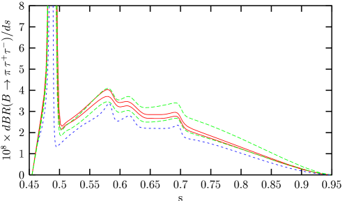
Figure 1: $dBR/ds$ for $B\rightarrow\pi\tau^{+}\tau^{-}$as a function of $s$ for $\bar{\xi}_{N,bb}^{D}=40\,m_{b}$ and $\bar{\xi}_{N,\tau\tau}^{D}=10\,m_{\tau}$, in case that the ratio $|r_{tb}|<1$. Here the region between the solid curves represents the $dBR/ds$ in Model III without the NHB effects, while the one between the dashed curves is for the $dBR/ds$ with NHB contributions. The SM prediction is represented by the small dashed curve

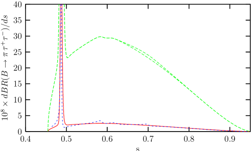
Figure 2: The same as Fig.(1), but for $r_{tb}>1$ with $\bar{\xi}_{N,bb}^{D}=0.1\,m_{b}$ and $\bar{\xi}_{N,\tau\tau}^{D}=m_{\tau}$.

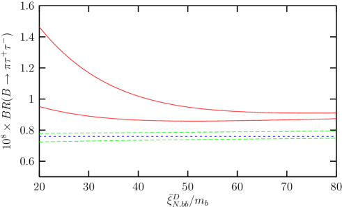
Figure 3: $BR$ of $B\rightarrow\pi\tau^{+}\tau^{-}$as a function of $\bar{\xi}_{N,bb}^{D}/m_{b}$ for $\bar{\xi}_{N,\tau\tau}^{D}=10\,m_{\tau}$ and $|r_{tb}|<1$. Here $BR$ is restricted in the region between solid (dashed) curves for $C^{eff}_{7}>0$ ($C^{eff}_{7}<0$). Small dashed straight line represents the SM prediction.

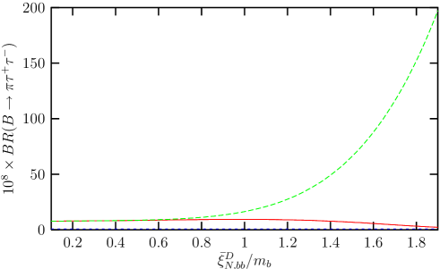
Figure 4: The same as Fig.(3), but for $r_{tb}>1$ with $\bar{\xi}_{N,\tau\tau}^{D}=m_{\tau}$.

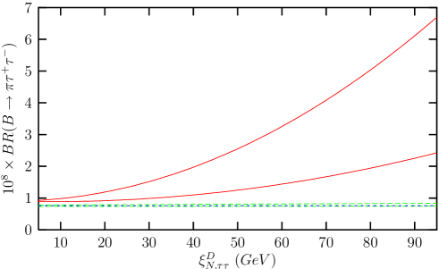
Figure 5: $BR$ of $B\rightarrow\pi\tau^{+}\tau^{-}$as a function of $\bar{\xi}_{N,\tau\tau}^{D}$ for $\bar{\xi}_{N,bb}^{D}=40\,m_{b}$ and $|r_{tb}|<1$. Here $BR$ is restricted in the region between solid (dashed) curves for $C^{eff}_{7}>0$ ($C^{eff}_{7}<0$). Small dashed straight line represents the SM prediction.

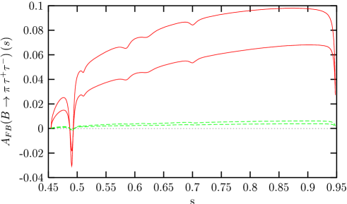
Figure 6: Differential $A_{FB}$ for $B\rightarrow\pi\tau^{+}\tau^{-}$as a function of $s$ for $\bar{\xi}_{N,bb}^{D}=40\,m_{b}$ and $\bar{\xi}_{N,\tau\tau}^{D}=10\,m_{\tau}$, in case of the ratio $|r_{tb}|<1$. Here differential $A_{FB}$ is restricted in the region between solid (dashed) curves for $C^{eff}_{7}>0$ ($C^{eff}_{7}<0$).

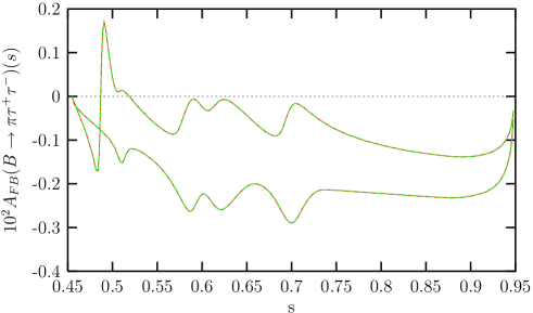
Figure 7: The same as Fig.(6), but for $r_{tb}>1$ with $\bar{\xi}_{N,bb}^{D}=0.1\,m_{b}$ and $\bar{\xi}_{N,\tau\tau}^{D}=m_{\tau}$.

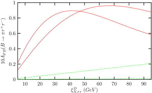
Figure 8: $A_{FB}$ for $B\rightarrow\pi\tau^{+}\tau^{-}$as a function of $\bar{\xi}_{N,\tau\tau}^{D}$ for $\bar{\xi}_{N,bb}^{D}=40\,m_{b}$ and $|r_{tb}|<1$. Here $A_{FB}$ is restricted in the region between solid (dashed) curves for $C^{eff}_{7}>0$ ($C^{eff}_{7}<0$).

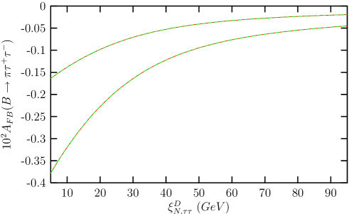
Figure 9: The same as Fig.(8), but for $r_{tb}>1$ with $\bar{\xi}_{N,bb}^{D}=0.1\,m_{b}$.

In Fig. (1), we plot the dependence of the $dBR/ds$ on the invariant dilepton mass $s$, for $|r_{tb}|<1$ and $C^{eff}_{7}>0$ cases, by taking into account the long distance effects. Here the region between the solid (red) curves represents the $dBR/ds$ in Model III without the NHB effects, while the one between the dashed (green) curves is for the $dBR/ds$ with NHB contributions. In both cases, we observe an enhancement compared to the SM prediction, which is represented by the small dashed (blue) curve. This enhancement reaches up to $70\,\%$ and $50\,\%$ as compared with the SM and the Model III prediction without NHB effects, respectively. In Fig. (2), the same comparison is made for $r_{tb}>1$ case and we see that the contributions coming from the NHB effects are extremely large. These figures explicitly show the size of the NHB effects on the exclusive $B\rightarrow\pi\tau^{+}\tau^{-}$decay.

From now on in figures we plot, the regions bounded by the solid (red) curves represent the $C_{7}^{eff}>0$ case and the regions bounded by the dashed (green) curves represent the $C_{7}^{eff}<0$ case while the small dashed (blue) curves are for the SM predictions for the relevant observable.

	$BR(B\rightarrow\pi\tau^{+}\tau^{-})$
$(\rho;\eta)$	$|V_{cb}|=0.037$	$|V_{cb}|=0.043$
$(0.3;0.34)$	$0.69\times 10^{-8}$	$0.93\times 10^{-8}$
$(-0.3;0.34)$	$0.60\times 10^{-8}$	$0.81\times 10^{-8}$
$(-0.07;0.34)$	$0.62\times 10^{-8}$	$0.83\times 10^{-8}$

Table 3: The values of the total branching ratio for $B\rightarrow\pi\tau^{+}\tau^{-}$decay in the SM, at three different sets of the Wolfenstein parameters $(\rho;\eta)$.

We present the dependence of the BR on the parameter $\bar{\xi}_{N,bb}^{D}/m_{b}$ in Figs.(3-4), where the first one is for $|r_{tb}|<1$ and the latter for $r_{tb}>1$. Our prediction for the BR of the $B\rightarrow\pi\tau^{+}\tau^{-}$decay in the SM including the long distance effects is

$$BR(B\rightarrow\pi\tau^{+}\tau^{-})=0.76\times 10^{-8}.$$ (42)

We also give the SM values of the total branching ratio for $B\rightarrow\pi\tau^{+}\tau^{-}$decay at three different sets of the Wolfenstein parameters $(\rho;\eta)$ in table 3. As seen from Fig. (3), for $|r_{tb}|<1$, the $C_{7}^{eff}<0$ case almost coincides with the SM prediction. However, for $C_{7}^{eff}>0$, we observe an enhancement which is $1.5-2$ times of the SM prediction; but this enhancement decreases with the increasing values of the $\bar{\xi}_{N,bb}^{D}/m_{b}$ parameter. In case of $r_{tb}>1$ (Fig. (4)), extremely large enhancement, $2-3$ orders larger compared the SM case, is reached for $C_{7}^{eff}<0$ case.

We plot the dependence of the BR on the parameter $\bar{\xi}_{N,\tau\tau}^{D}$ in Fig. (5) for $|r_{tb}|<1$ . From this figure, we again observe an enhancement as in the $\bar{\xi}_{N,bb}^{D}/m_{b}$ dependence and this is the contribution due to the NHB effects. However, the behavior of this dependence is opposite to that of $\bar{\xi}_{N,bb}^{D}/m_{b}$ dependence: the BR increases with the increasing values of the $\bar{\xi}_{N,\tau\tau}^{D}$. The SM prediction again lies in the region bounded by the $C_{7}^{eff}<0$ case.

The dependence of the differential $A_{FB}$ on the invariant dilepton mass $s$ for the $B\rightarrow\pi\tau^{+}\tau^{-}$decay is presented in Fig. (6) (Fig. (7)) for $|r_{tb}|<1$ ($r_{tb}>1$) case. Since $A_{FB}$ arises in the 2HDM only when the NHB effects are taken into account, it provides a good probe to test these effects. For $|r_{tb}|<1$, although $A_{FB}(s)$ is very small for $C_{7}^{eff}<0$ case, it is considerably enhanced for $C_{7}^{eff}>0$ case. For $r_{tb}>1$, $A_{FB}(s)$ for $C_{7}^{eff}<0$ and $C_{7}^{eff}>0$ cases completely coincide and its magnitude is one order smaller than the $|A_{FB}(s)|$ for $|r_{tb}|<1$ case.

Figs.(8) and (9) are devoted to the $\bar{\xi}_{N,\tau\tau}^{D}$ dependence of the $A_{FB}$ of the $B\rightarrow\pi\tau^{+}\tau^{-}$decay for $|r_{tb}|<1$ and $r_{tb}>1$ cases, respectively. As can be observed from Fig.(8), $A_{FB}$ is quite sensitive to the parameter $\bar{\xi}_{N,\tau\tau}^{D}$ especially for $C_{7}^{eff}>0$. It can reach 10% for $\bar{\xi}_{N,\tau\tau}^{D}\sim 60$. For $r_{tb}>1$ case shown in Fig.(9), the $C_{7}^{eff}<0$ and $C_{7}^{eff}>0$ cases completely coincide and $|A_{FB}|$ decreases with the increasing values of the $\bar{\xi}_{N,\tau\tau}^{D}$. In addition, its value is one order smaller than the $|r_{tb}|<1$ case.

3.2 Numerical results of the exclusive $B\rightarrow\rho\ell^{+}\ell^{-}$decay

In our numerical calculation for $B\rightarrow\rho\ell^{+}\ell^{-}$decay, we use three parameter fit of the light-cone QCD sum rule [30] which can be written in the following form

$$F(q^{2})=\frac{F(0)}{1-a_{F}~{}q^{2}/m_{B}^{2}+b_{F}(q^{2}/m_{B}^{2})^{2}}$$ (43)

where the values of the parameters $F(0)$, $a_{F}$ and $b_{F}$ are given in table (2). The form factors $A_{0}$ and $A_{3}$ can be found from the following parametrization,

$$A_{0} = A_{3}-\frac{T_{3}~{}q^{2}}{m_{\rho}m_{b}},$$

$$A_{3} = \frac{m_{B}+m_{\rho}}{2m_{\rho}}A_{1}-\frac{m_{B}-m_{\rho}}{2m_{\rho}}A_{2}.$$ (44)

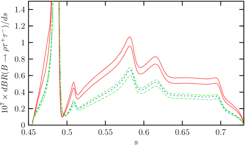
Figure 10: $dBR/ds$ for $B\rightarrow\rho\tau^{+}\tau^{-}$as a function of $s$ for $\bar{\xi}_{N,bb}^{D}=40\,m_{b}$ and $\bar{\xi}_{N,\tau\tau}^{D}=10\,m_{\tau}$, in case of the ratio $|r_{tb}|<1$. Here $dBR/ds$ is restricted in the region between solid (dashed) curves for $C^{eff}_{7}>0$ ($C^{eff}_{7}<0$. Small dashed curve represents the SM prediction.

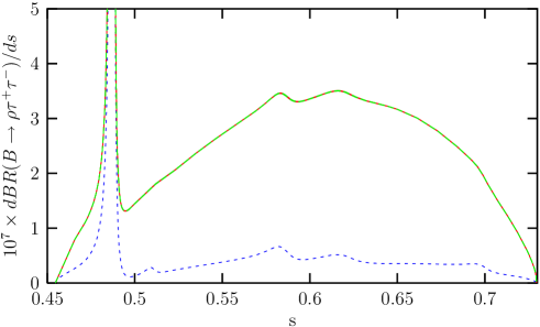
Figure 11: The same as Fig.(10), but for $r_{tb}>1$ with $\bar{\xi}_{N,bb}^{D}=0.1\,m_{b}$ and $\bar{\xi}_{N,\tau\tau}^{D}=m_{\tau}$.

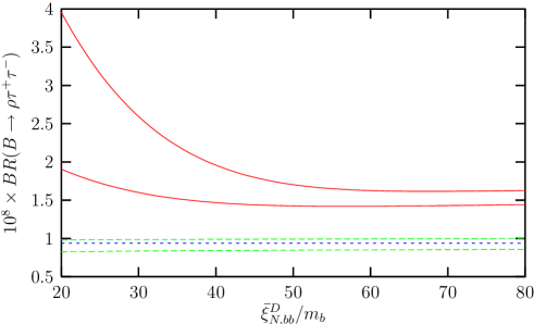
Figure 12: $BR$ for $B\rightarrow\rho\tau^{+}\tau^{-}$as a function of $\bar{\xi}_{N,bb}^{D}/m_{b}$ for $\bar{\xi}_{N,\tau\tau}^{D}=10\,m_{\tau}$ and $|r_{tb}|<1$. Here $BR$ is restricted in the region between solid (dashed) curves for $C^{eff}_{7}>0$ ($C^{eff}_{7}<0$). Small dashed straight line represents the SM prediction.

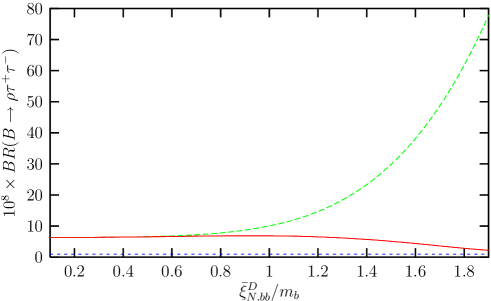
Figure 13: The same as Fig.(12), but for $r_{tb}>1$ with $\bar{\xi}_{N,\tau\tau}^{D}=m_{\tau}$.

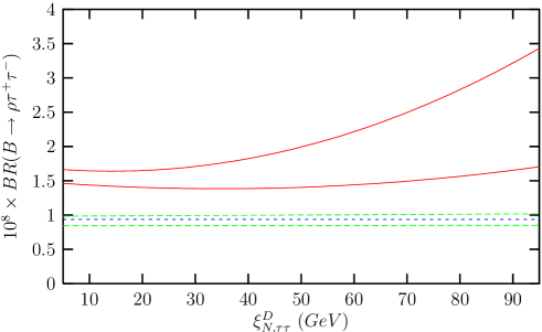
Figure 14: $BR$ for $B\rightarrow\rho\tau^{+}\tau^{-}$as a function of $\bar{\xi}_{N,\tau\tau}^{D}$ for $\bar{\xi}_{N,bb}^{D}=40\,m_{b}$ and $|r_{tb}|<1$. Here $BR$ is restricted in the region between solid (dashed) curves for $C^{eff}_{7}>0$ ($C^{eff}_{7}<0$). Small dashed straight line represents the SM prediction.

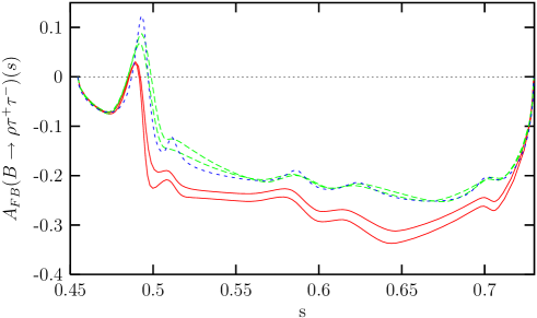
Figure 15: $A_{FB}(s)$ for $B\rightarrow\rho\tau^{+}\tau^{-}$as a function of $s$ for $\bar{\xi}_{N,bb}^{D}=40\,m_{b}$ and $\bar{\xi}_{N,\tau\tau}^{D}=10\,m_{\tau}$, in case of the ratio $|r_{tb}|<1$. Here $A_{FB}(s)$ is restricted in the region between solid (dashed) curves for $C^{eff}_{7}>0$ ($C^{eff}_{7}<0$). Small dashed curve represents the SM prediction.

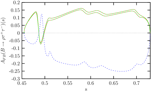
Figure 16: The same as Fig.(15), but for $r_{tb}>1$ with $\bar{\xi}_{N,bb}^{D}=0.1\,m_{b}$ and $\bar{\xi}_{N,\tau\tau}^{D}=m_{\tau}$.

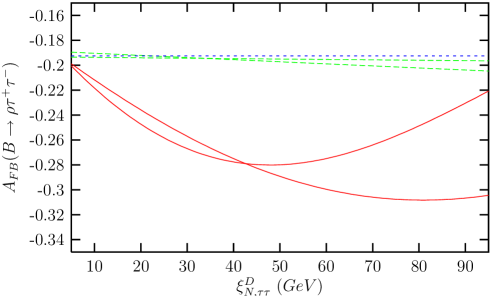
Figure 17: $A_{FB}$ for $B\rightarrow\rho\tau^{+}\tau^{-}$as a function of $\bar{\xi}_{N,\tau\tau}^{D}$ for $\bar{\xi}_{N,bb}^{D}=40\,m_{b}$ and $|r_{tb}|<1$. Here $A_{FB}$ is restricted in the region between solid (dashed) curves for $C^{eff}_{7}>0$ ($C^{eff}_{7}<0$). Small dashed straight line represents the SM prediction.

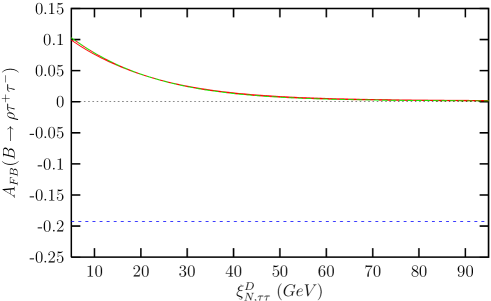
Figure 18: The same as Fig.(17), but for $r_{tb}>1$ with $\bar{\xi}_{N,bb}^{D}=0.1\,m_{b}$.

We first consider the dependence of $dBR/ds$ on the invariant dilepton mass $s$ for the $B\rightarrow\rho\tau^{+}\tau^{-}$decay. This is plotted in Fig.(10) for $\bar{\xi}^{D}_{N,bb}=40~{}m_{b}$ and $\bar{\xi}^{D}_{N,\tau\tau}=10~{}m_{\tau}$, in case of the ratio $|r_{tb}|<1$ by taking into account the long distance effects. We conclude from this graph that, $dBR/ds$ almost coincides with the SM result for $C_{7}^{eff}<0$ case, while for $C_{7}^{eff}>0$ it is considerably enhanced. As for the $r_{tb}>1$ case (Fig. (11))where we take $\bar{\xi}^{D}_{N,bb}=0.1~{}m_{b}$ and $\bar{\xi}^{D}_{N,\tau\tau}=m_{\tau}$, we observe an enhancement of one order as compared with the $|r_{tb}|<1$ and also the SM cases. Here $C_{7}^{eff}>0$ and $C_{7}^{eff}<0$ cases completely coincide.

	$BR(B\rightarrow\rho\tau^{+}\tau^{-})$		$A_{FB}(B\rightarrow\rho\tau^{+}\tau^{-})$
$(\rho;\eta)$	$|V_{cb}|=0.037$	$|V_{cb}|=0.043$
$(0.3;0.34)$	$0.94\times 10^{-8}$	$1.26\times 10^{-8}$	-0.17
$(-0.3;0.34)$	$0.72\times 10^{-8}$	$0.97\times 10^{-8}$	-0.20
$(-0.07;0.34)$	$0.76\times 10^{-8}$	$1.02\times 10^{-8}$	-0.19

Table 4: The values of the total branching ratio and the forward-backward asymmetry for $B\rightarrow\rho\tau^{+}\tau^{-}$decay in the SM, at three different sets of the Wolfenstein parameters $(\rho;\eta)$.

The dependence of the BR on one of the free parameters of the model III, $\bar{\xi}_{N,bb}^{D}/m_{b}$, is given in Figs. (12) and (13) for $|r_{tb}|<1$ and $r_{tb}>1$, respectively. Our prediction for the BR of the $B\rightarrow\rho\tau^{+}\tau^{-}$decay in the SM including the long distance effects is

$$BR(B\rightarrow\rho\tau^{+}\tau^{-})=0.94\times 10^{-8}.$$ (45)

We also give the SM values of the total branching ratio together with $A_{FB}$ values for $B\rightarrow\rho\tau^{+}\tau^{-}$decay at three different sets of the Wolfenstein parameters $(\rho;\eta)$ in table 4. As seen from Fig. (12), for $|r_{tb}|<1$ where we take $\bar{\xi}_{N,\tau\tau}^{D}=10\,m_{\tau}$, the $C_{7}^{eff}<0$ case coincides with the SM prediction. When $C_{7}^{eff}>0$, however, the BR is enhanced by $2.5-5$ times of the SM prediction; but this enhancement decreases with the increasing values of the $\bar{\xi}_{N,bb}^{D}/m_{b}$ parameter. For $r_{tb}>1$, we take $\bar{\xi}_{N,\tau\tau}^{D}=\,m_{\tau}$ and observe an enhancement for both $C_{7}^{eff}<0$ and $C_{7}^{eff}>0$ cases. For $C_{7}^{eff}<0$, it is one order larger than the SM value while for $C_{7}^{eff}>0$, the order of enhancement is the same as that in $|r_{tb}|<1$ case.

We plot the dependence of the BR on $\bar{\xi}_{N,\tau\tau}^{D}$, the other free parameter of model III, in Fig. (14) for $|r_{tb}|<1$. Here, we take $\bar{\xi}_{N,bb}^{D}=40\,m_{b}$ and see that the BR is not sensitive to $\bar{\xi}_{N,\tau\tau}^{D}$ for $C_{7}^{eff}<0$ and it is almost the same as the the SM prediction. However for $C_{7}^{eff}>0$, the BR is quite sensitive to $\bar{\xi}_{N,\tau\tau}^{D}$ and increases as it increases.

The dependence of $A_{FB}(s)$ of the $B\rightarrow\rho\tau^{+}\tau^{-}$decay on the invariant dilepton mass $s$ is represented in Fig.(15) (Fig.(16)) for $|r_{tb}|<1$ ($r_{tb}>1$) case. For $|r_{tb}|<1$, there is an enhancement on $|A_{FB}(s)|$ for $C_{7}^{eff}>0$, while for $C_{7}^{eff}<0$ it is almost the same as the SM prediction. For $r_{tb}>1$, all Model III predictions for $A_{FB}(s)$ almost coincide but with a flip in the sign as compared to the SM prediction.

Finally we present the dependence of the $A_{FB}$ on the $\bar{\xi}_{N,\tau\tau}^{D}$ parameter. Our prediction for the $A_{FB}$ of the $B\rightarrow\rho\tau^{+}\tau^{-}$decay in the SM is

$$A_{FB}(B\rightarrow\rho\,\tau^{+}\tau^{-})=\,-0.193$$ (46)

(See also table 4.) In Fig. (17), this dependence is plotted for the ratio $|r_{tb}|<1$ and $\bar{\xi}_{N,bb}^{D}=40\,m_{b}$. Although the $C_{7}^{eff}<0$ case almost coincides with the SM value, there is an enhancement for $|A_{FB}|$ up to the $50\%$ of the SM value for the moderate values of the $\bar{\xi}_{N,\tau\tau}^{D}$ parameter, for $C_{7}^{eff}>0$ case. For $r_{tb}>1$ case where we take $\bar{\xi}_{N,bb}^{D}=0.1\,m_{b}$, $|A_{FB}|$ can reach at most half of the SM value and drops to zero for large values of $\bar{\xi}_{N,\tau\tau}^{D}$. Here, $C_{7}^{eff}<0$ and $C_{7}^{eff}>0$ cases almost coincide.

Finally, we would like to comment briefly about the NHB effects on the CP violating asymmetry, $A_{CP}$, for $B\rightarrow\pi\ell^{+}\ell^{-}$and $B\rightarrow\rho\ell^{+}\ell^{-}$decays. As pointed out before [6]-[8], in the SM there is a considerable $A_{CP}$ in the partial rates for these decays because all three CKM factors contributing are at the same order. Further, the 2HDM contributions to $A_{CP}$ have been investigated in [9, 10] and it is shown that since charged Higgs contributions give rise to constructive interference to the SM result, $A_{CP}$ decreases while the BR increases for $B\rightarrow\pi\ell^{+}\ell^{-}$and $B\rightarrow\rho\ell^{+}\ell^{-}$decays in the 2HDM. We expect that including the NHB effects will further decrease magnitude of $A_{CP}$ with respect to its value without NHB effects. To see this, consider $A_{CP}$ between $B\rightarrow M\ell^{+}\ell^{-}$ and $B\rightarrow\bar{M}\ell^{+}\ell^{-}$ decays for $M=\pi,\rho$, which can be written as [20, 31]

$$A_{CP} \sim \frac{\int~{}ds~{}Im(C^{eff}_{7})Im(C^{eff}_{9}){\cal F}}{\int~{}ds~{}\Delta}$$

where ${\cal F}$ is a function of various form factors for the decays we consider and $\Delta$ is proportional to the one given by Eq.(24) and (34) for $\pi$ and $\rho$, respectively. As can be seen from the equation above, the numerator of the $A_{CP}$ ratio is free from the NHB contributions while the denominator gets this additional contribution so that magnitude of $A_{CP}$ will decrease with the inclusion of the NHB contributions.

3.3 Conclusion

In this paper we have investigated the physical observables, $BR$ and $A_{FB}$, related to the exclusive $B\rightarrow\pi\ell^{+}\ell^{-}$and $B\rightarrow\rho\ell^{+}\ell^{-}$decays in the general 2HDM including the NHB effects. We have found that NHB effects are quite sizable, leading to considerable enhancements on these physical observables. An experimental observation of the $A_{FB}$ in the $B\rightarrow\pi\ell^{+}\ell^{-}$decay, which is absent in the SM, would be a very powerful and direct test of the 2HDM and the existence of NHB. In conclusion we say that the exclusive $B\rightarrow\pi\ell^{+}\ell^{-}$and $B\rightarrow\rho\ell^{+}\ell^{-}$decays provide very useful testing ground for the new physics beyond the SM.

Appendix A The operator basis

The operator basis in the 2HDM for our process is [15, 32, 33]

$$O_{1} = (\bar{d}_{L\alpha}\gamma_{\mu}c_{L\beta})(\bar{c}_{L\beta}\gamma^{\mu}b_{L\alpha}),$$

$$O_{2} = (\bar{d}_{L\alpha}\gamma_{\mu}c_{L\alpha})(\bar{c}_{L\beta}\gamma^{\mu}b_{L\beta}),$$

$$O_{3} = (\bar{d}_{L\alpha}\gamma_{\mu}b_{L\alpha})\sum_{q=u,d,s,c,b}(\bar{q}_{L\beta}\gamma^{\mu}q_{L\beta}),$$

$$O_{4} = (\bar{d}_{L\alpha}\gamma_{\mu}b_{L\beta})\sum_{q=u,d,s,c,b}(\bar{q}_{L\beta}\gamma^{\mu}q_{L\alpha}),$$

$$O_{5} = (\bar{d}_{L\alpha}\gamma_{\mu}b_{L\alpha})\sum_{q=u,d,s,c,b}(\bar{q}_{R\beta}\gamma^{\mu}q_{R\beta}),$$

$$O_{6} = (\bar{d}_{L\alpha}\gamma_{\mu}b_{L\beta})\sum_{q=u,d,s,c,b}(\bar{q}_{R\beta}\gamma^{\mu}q_{R\alpha}),$$

$$O_{7} = \frac{e}{16\pi^{2}}\bar{d}_{\alpha}\sigma_{\mu\nu}(m_{b}R+m_{s}L)b_{\alpha}{\cal{F}}^{\mu\nu},$$

$$O_{8} = \frac{g}{16\pi^{2}}\bar{d}_{\alpha}T_{\alpha\beta}^{a}\sigma_{\mu\nu}(m_{b}R+m_{s}L)b_{\beta}{\cal{G}}^{a\mu\nu}\,\,,$$

$$O_{9} = \frac{e}{16\pi^{2}}(\bar{d}_{L\alpha}\gamma_{\mu}b_{L\alpha})(\bar{\ell}\gamma^{\mu}\ell)\,\,,$$

$$O_{10} = \frac{e}{16\pi^{2}}(\bar{d}_{L\alpha}\gamma_{\mu}b_{L\alpha})(\bar{\ell}\gamma^{\mu}\gamma_{5}\ell)\,\,,$$

$$O^{u}_{1} = (\bar{d}_{L\alpha}\gamma_{\mu}u_{L\beta})(\bar{u}_{L\beta}\gamma^{\mu}b_{L\alpha}),$$

$$O^{u}_{2} = (\bar{d}_{L\alpha}\gamma_{\mu}u_{L\alpha})(\bar{u}_{L\beta}\gamma^{\mu}b_{L\beta}),$$

$$Q_{1} = \frac{e^{2}}{16\pi^{2}}(\bar{d}^{\alpha}_{L}\,b^{\alpha}_{R})\,(\bar{\ell}\ell)\,,$$

$$Q_{2} = \frac{e^{2}}{16\pi^{2}}(\bar{d}^{\alpha}_{L}\,b^{\alpha}_{R})\,(\bar{\ell}\gamma_{5}\ell)\,,$$

$$Q_{3} = \frac{g^{2}}{16\pi^{2}}(\bar{d}^{\alpha}_{L}\,b^{\alpha}_{R})\,\sum_{q=u,d,s,c,b}(\bar{q}^{\beta}_{L}\,q^{\beta}_{R})\,,$$

$$Q_{4} = \frac{g^{2}}{16\pi^{2}}(\bar{d}^{\alpha}_{L}\,b^{\alpha}_{R})\,\sum_{q=u,d,s,c,b}(\bar{q}^{\beta}_{R}\,q^{\beta}_{L})\,,$$

$$Q_{5} = \frac{g^{2}}{16\pi^{2}}(\bar{d}^{\alpha}_{L}\,b^{\beta}_{R})\,\sum_{q=u,d,s,c,b}(\bar{q}^{\beta}_{L}\,q^{\alpha}_{R})\,,$$

$$Q_{6} = \frac{g^{2}}{16\pi^{2}}(\bar{d}^{\alpha}_{L}\,b^{\beta}_{R})\,\sum_{q=u,d,s,c,b}(\bar{q}^{\beta}_{R}\,q^{\alpha}_{L})\,,$$

$$Q_{7} = \frac{g^{2}}{16\pi^{2}}(\bar{d}^{\alpha}_{L}\,\sigma^{\mu\nu}\,b^{\alpha}_{R})\,\sum_{q=u,d,s,c,b}(\bar{q}^{\beta}_{L}\,\sigma_{\mu\nu}q^{\beta}_{R})\,,$$

$$Q_{8} = \frac{g^{2}}{16\pi^{2}}(\bar{d}^{\alpha}_{L}\,\sigma^{\mu\nu}\,b^{\alpha}_{R})\,\sum_{q=u,d,s,c,b}(\bar{q}^{\beta}_{R}\,\sigma_{\mu\nu}q^{\beta}_{L})\,,$$

$$Q_{9} = \frac{g^{2}}{16\pi^{2}}(\bar{d}^{\alpha}_{L}\,\sigma^{\mu\nu}\,b^{\beta}_{R})\,\sum_{q=u,d,s,c,b}(\bar{q}^{\beta}_{L}\,\sigma_{\mu\nu}q^{\alpha}_{R})\,,$$

$$Q_{10} = \frac{g^{2}}{16\pi^{2}}(\bar{d}^{\alpha}_{L}\,\sigma^{\mu\nu}\,b^{\beta}_{R})\,\sum_{q=u,d,s,c,b}(\bar{q}^{\beta}_{R}\,\sigma_{\mu\nu}q^{\alpha}_{L})\,,$$ (47)

where $\alpha$ and $\beta$ are $SU(3)$ colour indices and ${\cal{F}}^{\mu\nu}$ and ${\cal{G}}^{\mu\nu}$ are the field strength tensors of the electromagnetic and strong interactions, respectively.

Appendix B The initial values of the Wilson coefficients.

The initial values of the Wilson coefficients for the relevant process in the SM are [32]

$$C^{SM}_{1,3,\dots 6}(m_{W}) = 0\,\,,$$

$$C^{SM}_{2}(m_{W}) = 1\,\,,$$

$$C_{7}^{SM}(m_{W}) = \frac{3x_{t}^{3}-2x_{t}^{2}}{4(x_{t}-1)^{4}}\ln x_{t}+\frac{-8x_{t}^{3}-5x_{t}^{2}+7x_{t}}{24(x_{t}-1)^{3}}\,\,,$$

$$C_{8}^{SM}(m_{W}) = -\frac{3x_{t}^{2}}{4(x_{t}-1)^{4}}\ln x_{t}+\frac{-x_{t}^{3}+5x_{t}^{2}+2x_{t}}{8(x_{t}-1)^{3}}\,\,,$$

$$C_{9}^{SM}(m_{W}) = -\frac{1}{sin^{2}\theta_{W}}B(x_{t})+\frac{1-4\sin^{2}\theta_{W}}{\sin^{2}\theta_{W}}C(x_{t})-D(x_{t})+\frac{4}{9},\,\,,$$

$$C_{10}^{SM}(m_{W}) = \frac{1}{\sin^{2}\theta_{W}}(B(x_{t})-C(x_{t}))\,\,,$$

$$C_{Q_{i}}^{SM}(m_{W}) = 0~{}~{}~{}i=1,..,10$$ (48)

and for the additional part due to charged Higgs bosons are

$$C^{H}_{1,\dots 6}(m_{W}) = 0\,,$$

$$C_{7}^{H}(m_{W}) = Y^{2}\,F_{1}(y_{t})\,+\,XY\,F_{2}(y_{t})\,\,,$$

$$C_{8}^{H}(m_{W}) = Y^{2}\,G_{1}(y_{t})\,+\,XY\,G_{2}(y_{t})\,\,,$$

$$C_{9}^{H}(m_{W}) = Y^{2}\,H_{1}(y_{t})\,\,,$$

$$C_{10}^{H}(m_{W}) = Y^{2}\,L_{1}(y_{t})\,\,,$$ (49)

where

$$X = \frac{1}{m_{b}}~{}~{}~{}\left(\bar{\xi}^{D}_{N,bb}+\bar{\xi}^{D}_{N,db}\frac{V_{td}}{V_{tb}}\right)~{}~{},~{}~{}$$

$$Y = \frac{1}{m_{t}}~{}~{}~{}\left(\bar{\xi}^{U}_{N,tt}+\bar{\xi}^{U}_{N,tc}\frac{V^{*}_{cd}}{V^{*}_{td}}\right)~{}~{}.~{}~{}$$ (50)

Note that the results for model I and II can be obtained from model III by the following substitutions:

$$Y\rightarrow\cot\beta\,\, \,\,XY\rightarrow-\cot^{2}\beta\,\,for\,\,model\,I$$ ,

$$Y\rightarrow\cot\beta\,\, \,\,XY\rightarrow 1\,\,for\,\,model\,II\,.$$ ,

The NHB effects bring new operators and the corresponding Wilson coefficients read as [11]

$$C^{A^{0}}_{Q_{2}}((\bar{\xi}^{U}_{N,tt})^{3}) = \frac{\bar{\xi}^{D}_{N,\tau\tau}(\bar{\xi}^{U}_{N,tt})^{3}m_{b}y_{t}(\Theta_{5}(y_{t})z_{A}-\Theta_{1}(z_{A},y_{t}))}{32\pi^{2}m_{A^{0}}^{2}m_{t}\Theta_{1}(z_{A},y_{t})\Theta_{5}(y_{t})},$$

$$C^{A^{0}}_{Q_{2}}((\bar{\xi}^{U}_{N,tt})^{2}) = \frac{\bar{\xi}^{D}_{N,\tau\tau}(\bar{\xi}^{U}_{N,tt})^{2}\bar{\xi}^{D}_{N,bb}}{32\pi^{2}m_{A^{0}}^{2}}\Big{(}\frac{1}{\Theta_{1}(z_{A},y_{t})\Theta_{1}(z_{A},y_{t})\Theta_{5}(y_{t})}\Big{)}$$

$$\cdot (y_{t}(\Theta_{1}(z_{A},y_{t})-\Theta_{5}(y_{t})(xy+z_{A}))-2\Theta_{1}(z_{A},y_{t})\Theta_{5}(y_{t})\ln[\frac{z_{A}\Theta_{5}(y_{t})}{\Theta_{1}(z_{A},y_{t})}])$$

$$C^{A^{0}}_{Q_{2}}(\bar{\xi}^{U}_{N,tt}) = \frac{g^{2}\bar{\xi}^{D}_{N,\tau\tau}\bar{\xi}^{U}_{N,tt}m_{b}x_{t}}{64\pi^{2}m_{A^{0}}^{2}m_{t}}\Bigg{(}\frac{2}{\Theta_{5}(x_{t})}-\frac{xyx_{t}+2z_{A}}{\Theta_{1}(z_{A},x_{t})}-2\ln[\frac{z_{A}\Theta_{5}(x_{t})}{\Theta_{1}(z_{A},x_{t})}]$$

$$- xyx_{t}y_{t}(\frac{(x-1)x_{t}(y_{t}/z_{A}-1)-(1+x)y_{t})}{(\Theta_{6}-(x-y)(x_{t}-y_{t}))(\Theta_{3}(z_{A})+(x-y)(x_{t}-y_{t})z_{A})}$$

$$- \frac{x(y_{t}+x_{t}(1-y_{t}/z_{A}))-2y_{t}}{\Theta_{6}\Theta_{3}(z_{A})})\Bigg{)}$$

$$\!\!\!C^{A^{0}}_{Q_{2}}(\bar{\xi}^{D}_{N,bb}) = \frac{g^{2}\bar{\xi}^{D}_{N,\tau\tau}\bar{\xi}^{D}_{N,bb}}{64\pi^{2}m^{2}_{A^{0}}}\Big{(}1-\frac{x^{2}_{t}y_{t}+2y(x-1)x_{t}y_{t}-z_{A}(x^{2}_{t}+\Theta_{6})}{\Theta_{3}(z_{A})}$$

$$+ \frac{x^{2}_{t}(1-y_{t}/z_{A})}{\Theta_{6}}+2\ln[\frac{z_{A}\Theta_{6}}{\Theta_{2}(z_{A},x)}]\Big{)}$$

$$\!\!\!\!\!\!\!\!\!\!\!\!\!\!\!\!\!\!\!\!\!C^{H^{0}}_{Q_{1}}((\bar{\xi}^{U}_{N,tt})^{2})=\frac{g^{2}(\bar{\xi}^{U}_{N,tt})^{2}m_{b}m_{\tau}}{64\pi^{2}m^{2}_{H^{0}}m^{2}_{t}}\Bigg{(}\frac{x_{t}(1-2y)y_{t}}{\Theta_{5}(y_{t})}+\frac{(-1+2\cos^{2}\theta_{W})(-1+x+y)y_{t}}{\cos^{2}\theta_{W}\Theta_{4}(y_{t})}$$

$$+\frac{z_{H}(\Theta_{1}(z_{H},y_{t})xy_{t}+\cos^{2}\theta_{W}\,(-2x^{2}(-1+x_{t})yy^{2}_{t}+xx_{t}yy^{2}_{t}-\Theta_{8}z_{H}))}{\cos^{2}\theta_{W}\Theta_{1}(z_{H},y_{t})\Theta_{7}}\Bigg{)},$$

$$C^{H^{0}}_{Q_{1}}(\bar{\xi}^{U}_{N,tt}) = \frac{g^{2}\bar{\xi}^{U}_{N,tt}\bar{\xi}^{D}_{N,bb}m_{\tau}}{64\pi^{2}m^{2}_{H^{0}}m_{t}}\Bigg{(}\frac{(-1+2\cos^{2}\theta_{W})\,y_{t}}{\cos^{2}\theta_{W}\,\Theta_{4}(y_{t})}-\frac{x_{t}y_{t}}{\Theta_{5}(y_{t})}+\frac{x_{t}y_{t}(xy-z_{H})}{\Theta_{1}(z_{H},y_{t})}$$ (51)

$$+ \frac{(-1+2\cos^{2}\theta_{W})y_{t}z_{H}}{\cos^{2}\theta_{W}\Theta_{7}}-2x_{t}\,\ln\Bigg{[}\frac{\Theta_{5}(y_{t})z_{H}}{\Theta_{1}(z_{H},y_{t})}\Bigg{]}\Bigg{)},$$

$$C^{H^{0}}_{Q_{1}}(g^{4})=-\frac{g^{4}m_{b}m_{\tau}x_{t}}{128\pi^{2}m^{2}_{H^{0}}m^{2}_{t}}\Bigg{(}-1+\frac{(-1+2x)x_{t}}{\Theta_{5}(x_{t})+y(1-x_{t})}+\frac{2x_{t}(-1+(2+x_{t})y)}{\Theta_{5}(x_{t})}$$

$$-\frac{4\cos^{2}\theta_{W}(-1+x+y)+x_{t}(x+y)}{\cos^{2}\theta_{W}\Theta_{4}(x_{t})}+\frac{x_{t}(x(x_{t}(y-2z_{H})-4z_{H})+2z_{H})}{\Theta_{1}(z_{H},x_{t})}$$

$$+\frac{y_{t}((-1+x)x_{t}z_{H}+\cos^{2}\theta_{W}((3x-y)z_{H}+x_{t}(2y(x-1)-z_{H}(2-3x-y))))}{\cos^{2}\theta_{W}(\Theta_{3}(z_{H})+x(x_{t}-y_{t})z_{H})}$$

$$+2\,(x_{t}\ln\Bigg{[}\frac{\Theta_{5}(x_{t})z_{H}}{\Theta_{1}(z_{H},x_{t})}\Bigg{]}+\ln\Bigg{[}\frac{x(y_{t}-x_{t})z_{H}-\Theta_{3}(z_{H})}{(\Theta_{5}(x_{t})+y(1-x_{t})y_{t}z_{H}}\Bigg{]})\Bigg{)},$$

$$C^{h_{0}}_{Q_{1}}((\bar{\xi}^{U}_{N,tt})^{3}) = -\frac{\bar{\xi}^{D}_{N,\tau\tau}(\bar{\xi}^{U}_{N,tt})^{3}m_{b}y_{t}}{32\pi^{2}m_{h^{0}}^{2}m_{t}\Theta_{1}(z_{h},y_{t})\Theta_{5}(y_{t})}\Big{(}\Theta_{1}(z_{h},y_{t})(2y-1)+\Theta_{5}(y_{t})(2x-1)z_{h}\Big{)}$$

$$C^{h_{0}}_{Q_{1}}((\bar{\xi}^{U}_{N,tt})^{2}) = \frac{\bar{\xi}^{D}_{N,\tau\tau}(\bar{\xi}^{U}_{N,tt})^{2}}{32\pi^{2}m_{h^{0}}^{2}}\Bigg{(}\frac{(\Theta_{5}(y_{t})z_{h}(y_{t}-1)(x+y-1)-\Theta_{1}(z_{h},y_{t})(\Theta_{5}(y_{t})+y_{t})}{\Theta_{1}(z_{h})\Theta_{5}(y_{t})}$$

$$- 2\ln\Bigg{[}\frac{z_{h}\Theta_{5}(y_{t})}{\Theta_{1}(z_{h})}\Bigg{]}\Bigg{)}$$

$$C^{h^{0}}_{Q_{1}}(\bar{\xi}^{U}_{N,tt}) = -\frac{g^{2}\bar{\xi}^{D}_{N,\tau\tau}\bar{\xi}^{U}_{N,tt}m_{b}x_{t}}{64\pi^{2}m^{2}_{h^{0}}m_{t}}\Bigg{(}\frac{2(-1+(2+x_{t})y)}{\Theta_{5}(x_{t})}-\frac{x_{t}(x-1)(y_{t}-z_{h})}{\Theta^{\prime}_{2}(z_{h})}+2\ln\Bigg{[}\frac{z_{h}\Theta_{5}(x_{t})}{\Theta_{1}(z_{h},x_{t})}\Bigg{]}$$

$$+ \frac{x(x_{t}(y-2z_{h})-4z_{h})+2z_{h}}{\Theta_{1}(z_{h},x_{t})}-\frac{(1+x)y_{t}z_{h}}{xyx_{t}y_{t}+z_{h}((x-y)(x_{t}-y_{t})-\Theta_{6})}$$

$$+ \frac{\Theta_{9}+y_{t}z_{h}((x-y)(x_{t}-y_{t})-\Theta_{6})(2x-1)}{z_{h}\Theta_{6}(\Theta_{6}-(x-y)(x_{t}-y_{t}))}+\frac{x(y_{t}z_{h}+x_{t}(z_{h}-y_{t}))-2y_{t}z_{h}}{\Theta_{2}(z_{h})}\Bigg{)},$$

$$C^{h^{0}}_{Q_{1}}(\bar{\xi}^{D}_{N,bb}) = -\frac{g^{2}\bar{\xi}^{D}_{N,\tau\tau}\bar{\xi}^{D}_{N,bb}}{64\pi^{2}m^{2}_{h^{0}}}\Bigg{(}\frac{yx_{t}y_{t}(xx^{2}_{t}(y_{t}-z_{h})+\Theta_{6}z_{h}(x-2))}{z_{h}\Theta_{2}(z_{h})\Theta_{6}}+2\ln\Bigg{[}\frac{\Theta_{6}}{x_{t}y_{t}}\Bigg{]}$$

$$+ 2\ln\Bigg{[}\frac{x_{t}y_{t}z_{h}}{\Theta_{2}(z_{h})}\Bigg{]}\Bigg{)}$$

where

$$\Theta_{1}(\omega,\lambda) = -(-1+y-y\lambda)\omega-x(y\lambda+\omega-\omega\lambda)$$

$$\Theta_{2}(\omega) = (x_{t}+y(1-x_{t}))y_{t}\omega-xx_{t}(yy_{t}+(y_{t}-1)\omega)$$

$$\Theta^{\prime}_{2}(\omega) = \Theta_{2}(\omega,x_{t}\leftrightarrow y_{t})$$

$$\Theta_{3}(\omega) = (x_{t}(-1+y)-y)y_{t}\omega+xx_{t}(yy_{t}+\omega(-1+y_{t}))$$

$$\Theta_{4}(\omega) = 1-x+x\omega$$

$$\Theta_{5}(\lambda) = x+\lambda(1-x)$$

$$\Theta_{6} = (x_{t}+y(1-x_{t}))y_{t}+xx_{t}(1-y_{t})$$

$$\Theta_{7} = (y(y_{t}-1)-y_{t})z_{H}+x(yy_{t}+(y_{t}-1)z_{H})$$ (52)

$$\Theta_{8} = y_{t}(2x^{2}(1+x_{t})(y_{t}-1)+x_{t}(y(1-y_{t})+y_{t})+x(2(1-y+y_{t})$$

$$+ x_{t}(1-2y(1-y_{t})-3y_{t})))$$

$$\Theta_{9} = -x^{2}_{t}(-1+x+y)(-y_{t}+x(2y_{t}-1))(y_{t}-z_{h})-x_{t}y_{t}z_{h}(x(1+2x)-2y)$$

$$+ y^{2}_{t}(x_{t}(x^{2}-y(1-x))+(1+x)(x-y)z_{h})$$

and

$$x_{t}=\frac{m_{t}^{2}}{m_{W}^{2}}~{}~{}~{},~{}~{}~{}y_{t}=\frac{m_{t}^{2}}{m_{H^{\pm}}}~{}~{}~{},~{}~{}~{}z_{H}=\frac{m_{t}^{2}}{m^{2}_{H^{0}}}~{}~{}~{},~{}~{}~{}z_{h}=\frac{m_{t}^{2}}{m^{2}_{h^{0}}}~{}~{}~{},~{}~{}~{}z_{A}=\frac{m_{t}^{2}}{m^{2}_{A^{0}}}~{}~{}~{},~{}~{}~{}$$

The explicit forms of the functions $F_{1(2)}(y_{t})$, $G_{1(2)}(y_{t})$, $H_{1}(y_{t})$ and $L_{1}(y_{t})$ in Eq.(49) are given as

$$F_{1}(y_{t}) = \frac{y_{t}(7-5y_{t}-8y_{t}^{2})}{72(y_{t}-1)^{3}}+\frac{y_{t}^{2}(3y_{t}-2)}{12(y_{t}-1)^{4}}\,\ln y_{t}\,\,,$$

$$F_{2}(y_{t}) = \frac{y_{t}(5y_{t}-3)}{12(y_{t}-1)^{2}}+\frac{y_{t}(-3y_{t}+2)}{6(y_{t}-1)^{3}}\,\ln y_{t}\,\,,$$

$$G_{1}(y_{t}) = \frac{y_{t}(-y_{t}^{2}+5y_{t}+2)}{24(y_{t}-1)^{3}}+\frac{-y_{t}^{2}}{4(y_{t}-1)^{4}}\,\ln y_{t}\,\,,$$

$$G_{2}(y_{t}) = \frac{y_{t}(y_{t}-3)}{4(y_{t}-1)^{2}}+\frac{y_{t}}{2(y_{t}-1)^{3}}\,\ln y_{t}\,\,,$$

$$H_{1}(y_{t}) = \frac{1-4sin^{2}\theta_{W}}{sin^{2}\theta_{W}}\,\,\frac{xy_{t}}{8}\,\left[\frac{1}{y_{t}-1}-\frac{1}{(y_{t}-1)^{2}}\ln y_{t}\right]$$

$$- y_{t}\left[\frac{47y_{t}^{2}-79y_{t}+38}{108(y_{t}-1)^{3}}-\frac{3y_{t}^{3}-6y_{t}+4}{18(y_{t}-1)^{4}}\ln y_{t}\right]\,\,,$$

$$L_{1}(y_{t}) = \frac{1}{sin^{2}\theta_{W}}\,\,\frac{xy_{t}}{8}\,\left[-\frac{1}{y_{t}-1}+\frac{1}{(y_{t}-1)^{2}}\ln y_{t}\right]\,\,.$$

Finally, the initial values of the coefficients in the model III are

$$C_{i}^{2HDM}(m_{W}) = C_{i}^{SM}(m_{W})+C_{i}^{H}(m_{W}),$$

$$C_{Q_{1}}^{2HDM}(m_{W}) = \int^{1}_{0}dx\int^{1-x}_{0}dy\,(C^{H^{0}}_{Q_{1}}((\bar{\xi}^{U}_{N,tt})^{2})+C^{H^{0}}_{Q_{1}}(\bar{\xi}^{U}_{N,tt})+C^{H^{0}}_{Q_{1}}(g^{4})+C^{h^{0}}_{Q_{1}}((\bar{\xi}^{U}_{N,tt})^{3})$$

$$+ C^{h^{0}}_{Q_{1}}((\bar{\xi}^{U}_{N,tt})^{2})+C^{h^{0}}_{Q_{1}}(\bar{\xi}^{U}_{N,tt})+C^{h^{0}}_{Q_{1}}(\bar{\xi}^{D}_{N,bb})),$$

$$C_{Q_{2}}^{2HDM}(m_{W}) = \int^{1}_{0}dx\int^{1-x}_{0}dy\,(C^{A^{0}}_{Q_{2}}((\bar{\xi}^{U}_{N,tt})^{3})+C^{A^{0}}_{Q_{2}}((\bar{\xi}^{U}_{N,tt})^{2})+C^{A^{0}}_{Q_{2}}(\bar{\xi}^{U}_{N,tt})+C^{A^{0}}_{Q_{2}}(\bar{\xi}^{D}_{N,bb}))$$

$$C_{Q_{3}}^{2HDM}(m_{W}) = \frac{m_{b}}{m_{\ell}\sin^{2}\theta_{W}}(C_{Q_{1}}^{2HDM}(m_{W})+C_{Q_{2}}^{2HDM}(m_{W}))$$

$$C_{Q_{4}}^{2HDM}(m_{W}) = \frac{m_{b}}{m_{\ell}\sin^{2}\theta_{W}}(C_{Q_{1}}^{2HDM}(m_{W})-C_{Q_{2}}^{2HDM}(m_{W}))$$

$$C_{Q_{i}}^{2HDM}(m_{W}) = 0\,\,,\,\,i=5,...,10.$$ (54)

Here, we present $C_{Q_{1}}$ and $C_{Q_{2}}$ in terms of the Feynman parameters $x$ and $y$ since the integrated results are extremely large. Using these initial values, we can calculate the coefficients $C_{i}^{2HDM}(\mu)$ and $C^{2HDM}_{Q_{i}}(\mu)$ at any lower scale in the effective theory with five quarks, namely $u,c,d,s,b$ similar to the SM case [33]-[36].

The Wilson coefficients playing the essential role in this process are $C_{7}^{2HDM}(\mu)$, $C_{9}^{2HDM}(\mu)$, $C_{10}^{2HDM}(\mu)$, $C^{2HDM}_{Q_{1}}(\mu)$ and $C^{2HDM}_{Q_{2}}(\mu)$. For completeness, in the following we give their explicit expressions.

$$C_{7}^{eff}(\mu) = C_{7}^{2HDM}(\mu)+Q_{d}\,(C_{5}^{2HDM}(\mu)+N_{c}\,C_{6}^{2HDM}(\mu))\,\,,$$

where the LO QCD corrected Wilson coefficient $C_{7}^{LO,2HDM}(\mu)$ is given by

$$C_{7}^{LO,2HDM}(\mu) = \eta^{16/23}C_{7}^{2HDM}(m_{W})+(8/3)(\eta^{14/23}-\eta^{16/23})C_{8}^{2HDM}(m_{W})\,\,$$ (55)

$$+ C_{2}^{2HDM}(m_{W})\sum_{i=1}^{8}h_{i}\eta^{a_{i}}\,\,,$$

and $\eta=\alpha_{s}(m_{W})/\alpha_{s}(\mu)$, $h_{i}$ and $a_{i}$ are the numbers which appear during the evaluation [36].

$C_{9}^{eff}(\mu)$ contains a perturbative part and a part coming from LD effects due to conversion of the real $\bar{c}c$ into lepton pair $\ell^{+}\ell^{-}$:

$$C_{9}^{eff}(\mu)=C_{9}^{pert}(\mu)+Y_{reson}(s)\,\,,$$ (56)

where

$$C_{9}^{pert}(\mu) = C_{9}^{2HDM}(\mu)$$

$$+ h(z,s)[3C_{1}(\mu)+C_{2}(\mu)+3C_{3}(\mu)+C_{4}(\mu)+3C_{5}(\mu)+C_{6}(\mu)$$

$$+ \lambda_{u}(3C_{1}+C_{2})]-\frac{1}{2}h(1,s)\left(4C_{3}(\mu)+4C_{4}(\mu)+3C_{5}(\mu)+C_{6}(\mu)\right)$$

$$- \frac{1}{2}h(0,s)\left[C_{3}(\mu)+3C_{4}(\mu)-\lambda_{u}(6C_{1}(\mu)+2C_{2}(\mu))\right]$$

$$+ \frac{2}{9}\left(3C_{3}(\mu)+C_{4}(\mu)+3C_{5}(\mu)+C_{6}(\mu)\right)\,\,,$$

and

$$Y_{reson}(s) = -\frac{3}{\alpha^{2}_{em}}\kappa\sum_{V_{i}=\psi_{i}}\frac{\pi\Gamma(V_{i}\rightarrow\ell^{+}\ell^{-})m_{V_{i}}}{q^{2}-m_{V_{i}}+im_{V_{i}}\Gamma_{V_{i}}}$$ (58)

$$\times [(3C_{1}(\mu)+C_{2}(\mu)+3C_{3}(\mu)+C_{4}(\mu)+3C_{5}(\mu)+C_{6}(\mu))$$

$$+ \lambda_{u}(3C_{1}(\mu)+C_{2}(\mu))]\,.$$

In Eq.(56), the functions $h(u,s)$ are given by

$$h(u,s) = -\frac{8}{9}\ln\frac{m_{b}}{\mu}-\frac{8}{9}\ln u+\frac{8}{27}+\frac{4}{9}x$$ (61)

$$-\frac{2}{9}(2+x)|1-x|^{1/2}\left\{\begin{array}[]{ll}\left(\ln\left|\frac{\sqrt{1-x}+1}{\sqrt{1-x}-1}\right|-i\pi\right),&\mbox{for }x\equiv\frac{4u^{2}}{s}<1\\ 2\arctan\frac{1}{\sqrt{x-1}},&\mbox{for }x\equiv\frac{4u^{2}}{s}>1,\end{array}\right.$$

$$h(0,s) = \frac{8}{27}-\frac{8}{9}\ln\frac{m_{b}}{\mu}-\frac{4}{9}\ln s+\frac{4}{9}i\pi\,\,,$$ (62)

with $u=\frac{m_{c}}{m_{b}}$. The phenomenological parameter $\kappa$ in Eq. (58) is taken as $2.3$. In Eqs. (B.10) and (58), the contributions of the coefficients $C_{1}(\mu)$, …., $C_{6}(\mu)$ are due to the operator mixing.

Finally, the Wilson coefficients $C_{Q_{1}}(\mu)$ and $C_{Q_{2}}(\mu)$ are given by [15]

$$C_{Q_{i}}(\mu)=\eta^{-12/23}\,C_{Q_{i}}(m_{W})~{},~{}i=1,2~{}.$$ (63)

References

- [1] Belle Collaboration, KEK-PROGRESS-REPORT-97-1 (1997).
- [2] BaBar Collaboration, SLAC-PUB-7951.
- [3] A. Ali, hep-ph/9606324 and references therein.
- [4] T. M. Aliev, D. A. Demir, E. Iltan and N. K. Pak, Phys. Rev. Phys. Rev., D54, (1996) 851.
- [5] D. S. Du and M. Z. Yang, Phys. Rev., D54, (1996) 882.
- [6] F. Krüger, L.M. Sehgal, Phys. Rev., D56, (1997) 5452.
- [7] F. Krüger, L.M. Sehgal, Phys. Rev., D55, (1997) 2799.
- [8] S. Bertolini, F. Borzumati, A. Masiero, and G. Ridolfi, Nucl. Phys., B353, (1991) 591.
- [9] T.M. Aliev, M. Savci, Phys. Rev., D60 (1999) 14005.
- [10] E. O. Iltan, Int. J. Mod. Phys., A14, (1999) 4365.
- [11] E. O. Iltan and G. Turan, Phys. Rev. D 63 (2001) 115007.
- [12] C. Bobeth, T. Ewerth, F. Krüger and J. Urban, Phys. Rev. D 64 (2001) 074014.
- [13] G. Erkol and G. Turan, hep-ph/0110017
- [14] G. Erkol and G. Turan, hep-ph/0112115
- [15] Y. B. Dai, C. S. Huang and H. W. Huang, Phys. Lett. B390 (1997) 257, erratum B513 (2001) 429 ; C. S. Huang, L. Wei, Q. S. Yan and S. H. Zhu, Phys. Rev. D63 (2001) 114021.
- [16] Z. Xiong and J. M. Yang. hep-ph/0105260
- [17] S. Glashow, S. Weinberg, Phys.Rev., D15 (1977) 1958.
-
[18]
T.P. Cheng and M. Sher,
Phys. Rev D 35, 3484 (1987);
ibid. D 44, 1461 (1991);
W.S. Hou, Phys. Lett. B 296, 179 (1992);
A. Antaramian, L. Hall, and A. Rasin, Phys. Rev. Lett 69, 1871 (1992);
L. Hall and S. Weinberg, Phys. Rev D 48, 979 (1993);
M.J. Savage, Phys. Lett B 266, 135 (1991). - [19] D. Atwood, L. Reina and A. Soni, Phys. Rev. D55 (1997) 3156
- [20] E. O. Iltan, hep-ph/0102061.
- [21] T. M. Aliev, M. K. Cakmak and M. Savci, Nucl. Phys. B 607 (2001) 305.
- [22] D. Buskulic, et all., ALEP Collaboration, Phys. Lett. B343 (1995) 444; J. Kalinowski, Phys. Lett. B245 (1990) 201; A. K. Grant, Phys. Rev. D51 (1995) 207.
- [23] M. Ciuchini, G. Degrassi, P. Gambino and G. F. Giudice, Nucl. Phys. B527, (1998) 21; F. M. Borzumati and C. Greub, Phys. Rev. D58 (1998) 074004.
- [24] A. Heister, et all., ALEPH Collaboration, CERN-EP/2001-095.
- [25] M. S. Alam, et all., CLEO Collaboration, in ICHEP98 Conference 1998; ALEPH Collaboration, R. Barate et all., Phys. Lett. B429 (1998) 169.
- [26] T. M. Aliev, E. O. Iltan, J. Phys. G. Nucl. Part. Phys. 25 (1999) 989.
- [27] D. Bowser-Chao, K. Cheung and W-Y. Keung, Phys. Rev. D59 (1999) 115006.
- [28] D. Melikhov and N. Nikitin, hep-ph/9609503.
- [29] D. Melikhov, Phys. Rev. D53 (1996) 2460.
- [30] P. Ball, J. High Energy Physics 09 (1998) 005; P. Ball, V. M. Braun, Phys. Rev. D58 (1998) 094016; T. M. Aliev, A. Özpineci, M.Savci, Phys. Rev. D56(1997) 4260.
- [31] E. O. Iltan, G. Turan and I. Turan hep-ph/0110017
- [32] B. Grinstein, R. Springer, and M. B. Wise, Nucl. Phys. B339 (1990) 269; R. Grigjanis, P.J. O’Donnell, M. Sutherland and H. Navelet, Phys. Lett. B213 (1988) 355; Phys. Lett. B286 (1992) , 413; G. Cella, G. Curci, G. Ricciardi and A. Viceré, Phys. Lett. B325 (1994) 227; Nucl. Phys. B431 (1994) 417.
- [33] M. Misiak, Nucl. Phys., B393 (1993) 23; erratum ibid. B439 (1995) 461.
- [34] C. S. Huang, Nucl.Phys.Proc.Suppl. 93 (2001) 73
- [35] T. M. Aliev, and E. Iltan Phys. Rev. D58 (1998) 095014.
- [36] A. J. Buras and M. Münz,Phys. Rev. D52 (1995) 186.