A Statistical Analysis of Hadron Spectrum:
Quantum Chaos in Hadrons

Abstract

The nearest-neighbor mass-spacing distribution of the meson and baryon spectrum (up to 2.5 GeV) is described by the Wigner surmise corresponding to the statistics of the Gaussian orthogonal ensemble of random matrix theory. This can be viewed as a manifestation of quantum chaos in hadrons.

Quarks are glued into colorless objects called hadrons, forming a large and complex hadron spectrum. This spectrum is the main source of information about the quark-gluon interactions in the confinement regime, and hadron spectroscopy has been receiving a lot of attention both theoretically and experimentally.

In the study of complex spectra in general, statistical methods proved to be useful. One of the early successes of statistical analysis was Wigner’s celebrated discovery of the fact that fluctuation properties of complex nuclear spectra are described by the Random Matrix Theory (RMT) Wigner ; Dyson ; Porter65 ; Mehta67 ; Brody:1981 . It was later realized that these properties, referred to as Wigner-Dyson properties, have a great deal of universality and appear in spectra of many physical systems, ranging from quantum dots Alh00 to lattice gauge theories Ver95 ; Ver00 ; Berg:2000be ; Bittner:2001aq .

In this Letter we show that the experimentally measured hadron spectrum has at least some Wigner-Dyson properties as well. Once this is established the link to the underlying dynamics is made via the Bohigas–Giannoni–Schmit (BGS) conjecture BGS83 , which states that the Wigner-Dyson properties are generic to spectra of the systems with a quantum analog of chaotic dynamics — the “quantum chaos” (see, e.g., Gut90 ; CaC95 ).

Recent theoretical work in lattice QCD Ver95 ; Ver00 ; Berg:2000be and quantum-mechanical Yang-Mills models Salasnich:1997cw ; Bittner:2001aq has already addressed the statistical properties of QCD spectrum as well as the quantum chaos aspects. Our findings will provide certain empirical support of these results and, hopefully, motivate further studies in this direction.

We look at the experimentally measured mass spectrum of hadrons up to 2.5 GeV taken from the Particle Data Group (PDG) Summary Tables pdg . More specifically, we consider $N$, $\Delta$, $\Lambda$, and $\Sigma$ baryons up to $N$(2200), and all the mesons listed in the Summary Tables up to $f_{2}(2340)$. In doing so we exclude the poorly known “one-star baryons.” We have only verified that they do not have a significant impact on our results.

The spectrum can be organized into multiplets, see Fig. 1, characterized by a set of definite quantum numbers (QNs): isospin, spin, parity, strangeness, baryon number, and, in the case of mesons, charge conjugation. Using these data we would like to examine the probability distribution of spacing (mass-splitting), $S_{i}=m_{i+1}-m_{i}$, between nearest-neighbor hadrons within one multiplet (same QNs). We thus do not need to consider channels with only a single state below 2.5 GeV.

Figure 1: Light hadron spectrum (excluding 1-star baryons) in the form of multiplets characterized by definite quantum numbers.

Each multiplet provides a number of spacings which are gathered into a common array of spacings. We actually will be considering three arrays: $\{S_{i}\}_{B}$, $\{S_{i}\}_{M}$, and $\{S_{i}\}_{H}=\{\{S_{i}\}_{B},\,\{S_{i}\}_{M}\}$ containing the spacings of, respectively, the baryon, the meson, and all multiplets. As usual, the mean spacing, $\left<S\right>=(1/N)\sum_{k=1}^{N}S_{k}$ is scaled out and we deal with dimensionless arrays:

$$\{s_{i}\}_{B} = \{S_{i}\}_{B}/\left<S\right>_{B}\,,$$

$$\{s_{i}\}_{M} = \{S_{i}\}_{M}/\left<S\right>_{M}\,,$$ (1)

$$\{s_{i}\}_{H} = \{S_{i}\}_{H}/\left<S\right>_{H}=\{\{S_{i}\}_{B}/\left<S\right>_{H},\,\{S_{i}\}_{M}/\left<S\right>_{H}\}.$$

The mean spacing values $\left<S\right>_{B,M,H}$ are computed in Table I.

Spectrum	$\left<S\right>$, in MeV
Baryon	289.8 $\pm$ 18.8
Meson	284.3 $\pm$ 35.8
Hadron	287.1 $\pm$ 27.3

Table 1: Mean mass spacing. The error bars stem from the PDG quoted errors.

Histograms of the resulting spacing distributions, $p(\{s_{i}\}_{B})$, $p(\{s_{i}\}_{M})$, and $p(\{s_{i}\}_{H})$ are presented in Fig. 2. The curves in the figure show the Poisson-like distribution [$p(s)=\exp(-s)$], and the Wigner surmise [$p(s)=\frac{\pi}{2}\,s\,\exp(-{\frac{\pi}{4}s^{2}})$]. They represent two extreme regimes: uncorrelated spectrum vs. a strongly correlated one.

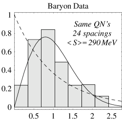
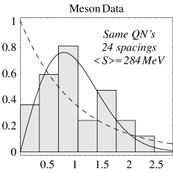
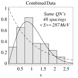
Figure 2: Histograms of the nearest-neighbor mass spacing distribution for hadron states with same QNs. Curves represent the Poisson (dashed) and Wigner (solid) distributions.

The figure clearly shows that the experimental distribution is of the Wigner-surmise type. We have checked that if one does not discriminate the QNs (“mixed QNs”) the spacing distribution is Poissonian, so only states with the same QNs are correlated.

The histogram plots represent the distributions in a rather qualitative way because due to the low statistics the picture is very sensitive to the choice of the grid. Accounting for the error bars makes it even less accurate. It is more instructive to consider integrated characteristics, such as the moments of distribution. For our empirical distribution the $n$-th moment is simply calculated as

$$\left<s^{n}\right>_{\rm exp}=\frac{1}{N}\sum\limits_{i=1}^{N}s_{i}^{n}\,,$$ (2)

which obviously is not sensitive to the analysis artifacts such as the choice of energy grid.

At the same time let us consider a more general form of the Wigner surmise:

$$p_{\rm W}(s)=As^{\beta}\exp(-Bs^{2})$$ (3)

where $\beta$ is a parameter — the Dyson index; $A$ and $B$ are constants fixed by the normalization conditions: $\left<s^{0}\right>_{\rm W}=1=\left<s^{1}\right>_{\rm W}$, where, naturally, $\left<s^{n}\right>_{\rm W}=\int_{0}^{\infty}ds\,s^{n}\,p_{\rm W}(s)$. Depending on the value of $\beta$ expression (3) approximates the spacing distributions of the RMT for various types of Gaussian ensembles. The most common values are $\beta=1,\,2$, and $4$ which represent the orthogonal (GOE), unitary (GUE), and symplectic (GSE) ensembles, respectively.

Figure 3: Moments of spacing distributions. Explanations on the data points are given in the text. Curves represent the moments of Poisson distribution (dashed), and of the Wigner surmise for GOE (solid), GUE (short-dashed), and GSE (long-dashed).

Computing the first ten, or so, moments of all the relevant distributions we obtain Figure 3. The moments of the Poisson and Wigner distributions (shown by lines) are proportional to the Gamma-function [e.g., $\left<s^{n}\right>_{P}=\Gamma(n+1)$, and $\left<s^{n}\right>_{W}=(2/\sqrt{\pi})^{n}\,\Gamma(\mbox{\small{$\frac{1}{2}$}}n+1)$, for $\beta=1$]. Therefore they all increase rapidly with $n$ and we have used logarithmic scale to plot them.

Data points in the first three panels correspond to the empirical distributions shown by the histograms in Fig. 2, now with the PDG error bars properly accounted for. The Wigner surmise with $\beta=1$ fits these distributions extremely well: comparing the first ten moments, $\chi^{2}/{\rm point}$ values for the three distributions are shown in the “None” row of Table 2.

In general, before combining the level statistics from two different spectra we would need to perform an unfolding of these spectra. Then the combined meson-baryon array of spacings could be constructed as $\{s_{i}\}_{H}^{\prime}=\{\{s_{i}\}_{B},\,\{s_{i}\}_{M}\}$. However, because the baryon and meson mean spacing come out so similar (Table I) this construction leads to practically same results as the one in Eq. (A Statistical Analysis of Hadron Spectrum: Quantum Chaos in Hadrons), the $\chi^{2}$ value changes insignificantly, see “B vs M” row of Table 2. One can also perform the unfolding with respect to strangeness, which means one treats the spectrum of strange baryons and mesons as different from that of non-strange ones, and unfolds (i.e., normalizes to unit mean spacing) prior combining them. In this case the agreement with Wigner surmise has slightly improved as is seen from the “S=0 vs $-1$” row of Table 2.

Unfolding	Baryon $\chi^{2}$	Meson $\chi^{2}$	Hadron $\chi^{2}$
None	0.52	0.66	0.57
B vs M	—	—	0.54
S=0 vs $-1$	0.29	0.40	0.33

Table 2: $\chi^{2}/point$ fit of $\beta=1$ Wigner surmise to the first ten moments of the experimental spacing distributions for various unfoldings.

To recapitulate, the hadron level-spacing distribution is remarkably well described by the Wigner surmise for $\beta=1$. This indicates that the fluctuation properties of the hadron spectrum fall into the GOE universality class, and hence hadrons exhibit the quantum chaos phenomenon. One then should be able to describe the statistical properties of hadron spectra using RMT with random Hamiltonians from GOE that are characterized by good time-reversal and rotational symmetry.

The hadron-exchange models (e.g.PaT00 ) should also be able benefit from the RMT methods, in a way analogous to the stochastic theory of compound-nucleus reactions Brody:1981 ; VWZ85 . However, since unitarity is an essential ingredient of such models, a study of hadron width distribution is in order. Widths of compound nuclei have the Porter–Thomas distribution Porter65 that eventually allows one to define the unitary $S$-matrix completely within the RMT. We anticipate that the same approach will be applicable in the hadron-exchange reactions once the hadron-width distribution is determined.

It would be interesting to see how quantum chaos emerges in hadrons as a result of quark-gluon underlying dynamics. Lattice QCD studies in this direction are underway Ver95 ; Ver00 ; Berg:2000be . This problem could also be addressed in a quark-model framework. In particular, does a quark-model Hamiltonians which fits the physical spectrum indeed defines a chaotic classical system?

In conclusion, we have examined the nearest-neighbor level-spacing (mass-splitting) distribution, $p(s)$, of the experimental hadron spectrum. We focused on the lighter part of the hadron spectrum ($m<2.5GeV$), since it is more reliably known. The mean level-spacing seems to be the only relevant scale here, and after it is scaled out the distribution shows universal behavior. Unfortunately, the masses and quantum numbers are well known only for a few dozen hadron states, so achieving high statistics is out of the question. Nonetheless, the low-statistics analysis we have performed pinpoints the moments of the distribution accurately enough to claim that hadronic $p(s)$ fits the Wigner surmise with linear level repulsion ($\beta=1$). This indicates that the spectrum falls into the GOE universality class of random matrix theory. Invoking the BGS conjecture, this result is viewed as an empirical evidence of the “quantum chaos” phenomenon in hadrons.

- (1) E. P. Wigner, Ann. Math. 53, 36 (1951); 62, 548 (1955); 65, 203 (1957); 67, 325 (1958).
- (2) F. J. Dyson, J. Math. Phys. 3, 140 (1962); 3, 157 (1962); 3, 166 (1962); 3, 1199 (1962).
- (3) C. E. Porter, Statistical Theory of Spectra: Fluctuations (Academic, New York, 1965), and references therein.
- (4) M. L. Mehta, Random Matrices and the Statistical Theory of Energy Levels (Academic, New York, 1967).
- (5) T. A. Brody, J. Flores, J. B. French, P. A. Mello, A. Pandey and S. S. Wong, Rev. Mod. Phys. 53, 385 (1981).
- (6) Y. Alhassid, Rev. Mod. Phys. 72, 895 (2000).
- (7) M. A. Halasz and J. J. M. Verbaarschot, Phys. Rev. Lett. 74, 3920 (1995); D. Toublan and J. J. M. Verbaarschot, Nucl. Phys. B 603, 343 (2001).
- (8) J. J. Verbaarschot, Nucl. Phys. Proc. Suppl. 90, 219 (2000).
- (9) B. A. Berg, E. Bittner, H. Markum, R. Pullirsch, M. P. Lombardo and T. Wettig, “Universality and chaos in quantum field theories,” arXiv:hep-lat/0007008.
- (10) E. Bittner, H. Markum and R. Pullirsch, ‘Quantum chaos in physical systems: From super conductors to quarks,” arXiv:hep-lat/0110222.
- (11) O. Bohigas, M. J. Giannoni and C. Schmit, Phys. Rev. Lett. 52, 1 (1984).
- (12) M. C. Gutzwiller, Chaos in Classical and Quantum Mechanics (Springer, Berlin, 1990).
- (13) G. Casati and B. V. Chirikov, Quantum Chaos (Cambridge U. P., Cambridge, 1995).
- (14) L. Salasnich, Mod. Phys. Lett. A 12, 1473 (1997).
- (15) D.E. Groom et. al., Eur. Phys. J. C15 1 (2000) [URL: http://pdg.lbl.gov].
- (16) R. U. Haq, A. Pandey, and O. Bohigas, Phys. Rev. Lett. 48, 1086 (1982).
- (17) V. Pascalutsa and J. A. Tjon, Phys. Rev. C 61, 054003 (2000); V. Pascalutsa, Hadronic J. Suppl. 16, 1 (2001).
- (18) J. J. Verbaarschot, H. A. Weidenmuller and M. R. Zirnbauer, Phys. Rept. 129, 367 (1985).