Abstract

We consider $J/\psi$ meson photoproduction on protons at high energies at the leading order in $\alpha_{s}$ using conventional parton model and $k_{\top}$-factorization approach of QCD. It is shown that in the both cases the colour singlet mechanism gives correct description for experimental data from HERA for the total cross section and for the $J/\psi$ meson z-spectrum at realistic values of a c-quark mass and meson wave function at the origin $\Psi(0)$. At the same time our predictions for $p_{\top}$-spectrum of $J/\psi$ meson and for $p_{\top}$ dependence of the spin parameter $\alpha$ obtained in $k_{\top}$-factorization approach are very different from the results obtained in conventional parton model. Such a way the experimental study of a polarized $J/\psi$ meson production at the large $p_{\top}$ should be a direct test of BFKL gluons.

1 Introduction

It is well known that in the processes of $J/\psi$ meson photoproduction on protons at high energies the photon-gluon fusion partonic subprocess dominates [1]. In the framework of general factorization approach of QCD the $J/\psi$ photoproduction cross section depends on the gluon distribution function in a proton, the hard amplitude of $c\bar{c}$-pair production as well as the mechanism of a creation colorless final state with quantum numbers of the $J/\psi$ meson. Such a way, we suppose that the soft interactions in the initial state are described by introducing a gluon distribution function, the hard partonic amplitude is calculated using perturbative theory of QCD at order in $\alpha_{s}(\mu^{2})$, where $\mu\sim m_{c}$, and the soft process of the $c\bar{c}$-pair transition into $J/\psi$ meson is described in nonrelativistic approximation using series in the small parameters $\alpha_{s}$ and $v$ (relative velocity of the quarks in $J/\psi$ meson). As it is statement in nonrelativistic QCD (NRQCD) [2], there are colour singlet mechanism, where $c\bar{c}$-pair is hardly produced in the colour singlet state, and colour octet mechanism, where $c\bar{c}$-pair is produced in the color octet state and at long distance it transforms into final colour singlet state in soft process. However, as it was shown in paper [3], the data from HERA collider [4] in the wide region of $p_{\top}$ and $z$ may be described well in the framework of the colour singlet model and not colour octet contribution is needed. Based on the above mentioned result we will take into account in our analysis only the colour singlet model contribution in the $J/\psi$ meson photoproduction [1]. We consider a role of a proton gluon distribution function in the $J/\psi$ photoproduction in the framework of the conventional parton model as well as in the framework of the $k_{\top}$-factorization approach [5]. Last one is based on BFKL evolution equation [6], which takes into account large terms proportional to $\log 1/x$ and $\log\mu^{2}/\Lambda_{QCD}^{2}$ opposite to DGLAP evolution equation [7], where only large logarithmic terms $\sim\log\mu^{2}/\Lambda_{QCD}^{2}$ are taken into account. In the process of the $J/\psi$ meson photoproduction one has $x\sim\mu^{2}/s$ and $\mu^{2}\sim M^{2}$, where $M$ is the $J/\psi$ meson mass, $s$ is the square of a total energy of colliding particles in center of mass frame.

2 The cross section for $\gamma p\to J/\psi X$ in $k_{\top}$-factorization approach

Nowadays, there are two approaches in calculating of $J/\psi$ meson or heavy quark production cross sections at high energies. In the conventional parton model [8] it is suggested that hadronic cross section $\sigma(\gamma p\to J/\psi X,s)$ and relevant partonic cross section $\hat{\sigma}(\gamma g\to J/\psi g,\hat{s})$ are connected as follows:

$$\sigma^{PM}(\gamma p\to J/\psi X,s)=\int dx\hat{\sigma}(\gamma g\to J/\psi g,\hat{s})G(x,\mu^{2}),$$ (1)

where $\hat{s}=xs$, $G(x,\mu^{2})$ is the collinear gluon distribution function in a proton, $x$ is the fraction of a proton momentum, $\mu^{2}$ is the typical scale of a hard process. The $\mu^{2}$ dependence of the gluon distribution $G(x,\mu^{2})$ is described by DGLAP evolution equation [7]. In the region of very high $s$ one has $x<<1$. This fact leads to BFKL evolution equation [6] for the unintegrated gluon distribution function $\Phi(x,\bf q_{\top}^{2},\mu^{2})$, where $\bf q_{\top}^{2}$ is the gluon virtuality. The unintegrated gluon distribution function can be related to the conventional gluon distribution by

$$xG(x,\mu^{2})=\int_{0}^{\mu^{2}}\Phi(x,{\bf q}_{\top}^{2},\mu^{2})d{\bf q}_{\top}^{2}.$$ (2)

The gluon 4-momentum is presented as follows

$$q=xp_{N}+q_{\top},$$

where $q_{\top}=(0,{\bf q}_{\top},0)$, $p_{N}=(E_{N},0,0,|{\bf p}_{N}|)$ and $q^{2}=q^{2}_{\top}=-{\bf q_{\top}}^{2}$. So called BFKL gluon is off mass-shell and it has polarization vector along its transverse momentum such as $\varepsilon^{\mu}=q_{\top}^{\mu}/|\bf q_{\top}|$. In $k_{\top}$-factorization approach hadronic and partonic cross sections are related by the following condition:

$$\sigma(\gamma p\to J/\psi X)=\int\frac{dx}{x}\int_{0}^{\mu^{2}}d{\bf q}^{2}_{\top}\int\frac{d\phi}{2\pi}\Phi(x,{\bf q}^{2}_{\top},\mu^{2})\hat{\sigma}(\gamma g^{*}\to J/\psi g,\hat{s},{\bf q}^{2}_{\top}),$$ (3)

where $\hat{\sigma}(\gamma g^{*}\to J/\psi g)$ is $J/\psi$ meson photoproduction on BFKL gluon, $\phi$ is azimuthal angle in the transverse $XY$ plane between vector ${\bf q}_{\top}$ and fixed $OX$ axis.

3 Unintegrated gluon distribution function

At the present time an exact form of the unintegrated gluon distribution $\Phi(x,{\bf q}^{2}_{\top},\mu^{2})$ is unknown yet because the relevant experimental analysis of the experimental data has never been carried out. There are several theoretical approximations for $\Phi(x,{\bf q}^{2}_{\top},\mu^{2})$, which are based on solving BFKL evolution equation [9, 10, 11, 14]. In the region of very small $x\leq 0.01$ and moderate ${\bf q}^{2}_{\top}$ ($\sim 10$ GeV²), which is relevant for $J/\Psi$ photoproduction at HERA, all parameterizations [9, 10, 14] are approximately coincide (see, for example, discussions in [12] and [13]). For our purposes, we will use the unintegrated gluon distribution, which was obtained in the paper [14]. The proposed method lies upon a straightforward perturbative solution of the BFKL equation where the collinear gluon density $G(x,\mu^{2})$ is used as the boundary condition in the integral form (2). Technically, the unintegrated gluon distribution is calculated as a convolution of collinear gluon distribution $G(x,\mu^{2})$ with universal weight factors:

$$\Phi(x,{\bf q}^{2}_{\top},\mu^{2})=\int_{x}^{1}{\cal G}(\eta,{\bf q}^{2}_{\top},\mu^{2})\frac{x}{\eta}G(\frac{x}{\eta},\mu^{2})d\eta,$$ (4)

where

$${\cal G}(\eta,{\bf q}^{2}_{\top},\mu^{2})=\frac{\bar{\alpha}_{s}}{\eta{\bf q}^{2}_{\top}}J_{0}\left[2\sqrt{\bar{\alpha}_{s}\ln(\frac{1}{\eta})\ln(\frac{\mu^{2}}{{\bf q}^{2}_{\top}})}\right],\mbox{ at }{\bf q}^{2}_{\top}\leq\mu^{2}$$ (5)

$${\cal G}(\eta,{\bf q}^{2}_{\top},\mu^{2})=\frac{\bar{\alpha}_{s}}{\eta{\bf q}^{2}_{\top}}I_{0}\left[2\sqrt{\bar{\alpha}_{s}\ln(\frac{1}{\eta})\ln(\frac{{\bf q}^{2}_{\top}}{\mu^{2}})}\right],\mbox{ at }{\bf q}^{2}_{\top}>\mu^{2},$$ (6)

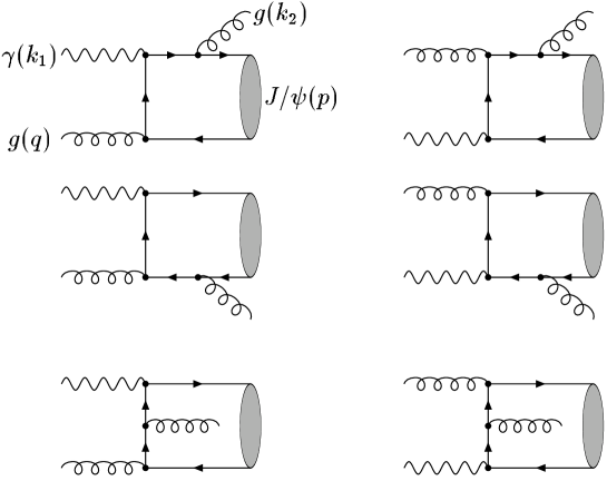
Figure 1: Diagrams used for description partonic process $\gamma+g\to J/\psi+g$.

$J_{0}$ and $I_{0}$ stand for Bessel functions (of real and imaginary arguments, respectively), and $\bar{\alpha}_{s}=\displaystyle{\frac{\alpha_{s}}{3\pi}}$. As a input function $G(x,\mu^{2})$ in (5,6) we use the standard GRV parameterization [15]. To test the method of calculation for $\Phi(x,{\bf q}^{2}_{\top},\mu^{2})$ we compare input collinear gluon distribution $G(x,\mu^{2})$ and collinear gluon distribution $\tilde{G}(x,\mu^{2})$, which is obtained using formula (2) from the unintegrated distribution $\Phi(x,{\bf q}^{2}_{\top},\mu^{2})$ after integration over ${\bf q}^{2}_{\top}$. In the Figure 1 the result of our calculation for the ratio $R_{1}(x,\mu^{2})=\tilde{G}(x,\mu^{2})/G(x,\mu^{2})$ is shown. It is visible, that at $x<0.1$ the ratio $R_{1}$ does not differ from 1 more than 1-2 %. Note, that in a process of the $J/\psi$ photoproduction on protons $x\sim\displaystyle{\frac{M}{\sqrt{s}}}$ ($M$ is the mass of $J/\psi$ meson), and one has $x\sim 0.03$ at $\sqrt{s}=100$ GeV.

4 Amplitude for $\gamma g\to J/\psi g$ process

There are six Feynman diagrams (Figure 2) which describere partonic process $\gamma g\to J/\psi g$ at the leading order in $\alpha_{s}$ and $\alpha$. In the framework of the colour singlet model and nonrelativistic approximation the production of $J/\psi$ meson is considered as the production of a quark-antiquark system in the colour singlet state with orbital momentum $L=0$ and spin momentum $S=1$. The binding energy and relative momentum of quarks in the $J/\psi$ are neglected. Such a way $M=2m_{c}$ and $p_{c}=p_{\bar{c}}=\displaystyle{\frac{p}{2}}$, where $p$ is 4-momentum of the $J/\psi$, $p_{c}$ and $p_{\bar{c}}$ are 4-momenta of quark and antiquark. Taking into account the formalism of the projection operator [16] the amplitude of the process $\gamma g\to J/\psi g$ may be obtained from the amplitude of the process $\gamma g\to\bar{c}cg$ after replacement:

$$V^{i}(p_{\bar{c}})\bar{U}^{j}(p_{c})\rightarrow\frac{\Psi(0)}{2\sqrt{M}}\hat{\varepsilon}(p)(\hat{p}+M)\frac{\delta^{ij}}{\sqrt{3}},$$ (7)

where $\hat{\varepsilon}(p)=\varepsilon_{\mu}(p)\gamma^{\mu}$, $\varepsilon_{\mu}(p)$ is 4-vector of the $J/\psi$ polarization, $\displaystyle{\frac{\delta^{ij}}{\sqrt{3}}}$ is the color factor, $\Psi(0)$ is the nonrelativistic meson wave function at the origin. The matrix elements of the process $\gamma g^{*}\to J/\psi g$ may be presented as follows:

$$M_{i}=KC^{ab}\varepsilon_{\alpha}(k_{1})\varepsilon^{a}_{\mu}(q)\varepsilon^{b}_{\beta}(k_{2})\varepsilon_{\nu}(p)M_{i}^{\alpha\beta\mu\nu},$$ (8)

$$M_{1}^{\alpha\beta\mu\nu}=\mbox{Tr}\left[\gamma^{\nu}(\hat{p}+M)\gamma^{\alpha}\frac{\hat{p}_{c}-\hat{k}_{1}+m_{c}}{(p_{c}-k_{1})^{2}-m_{c}^{2}}\gamma^{\mu}\frac{-\hat{p}_{\bar{c}}-\hat{k}_{2}+m_{c}}{(p_{\bar{c}}+k_{2})^{2}-m_{c}^{2}}\gamma^{\beta}\right]$$ (9)

$$M_{2}^{\alpha\beta\mu\nu}=\mbox{Tr}\left[\gamma^{\nu}(\hat{p}+M)\gamma^{\beta}\frac{\hat{p}_{c}+\hat{k}_{2}+m_{c}}{(p_{c}+k_{2})^{2}-m_{c}^{2}}\gamma^{\alpha}\frac{\hat{q}-\hat{p}_{\bar{c}}+m_{c}}{(q-p_{\bar{c}})^{2}-m_{c}^{2}}\gamma^{\mu}\right]$$ (10)

$$M_{3}^{\alpha\beta\mu\nu}=\mbox{Tr}\left[\gamma^{\nu}(\hat{p}+M)\gamma^{\alpha}\frac{\hat{p}_{c}-\hat{k}_{1}+m_{c}}{(p_{c}-k_{1})^{2}-m_{c}^{2}}\gamma^{\beta}\frac{\hat{q}-\hat{p}_{\bar{c}}+m_{c}}{(q-p_{\bar{c}})^{2}-m_{c}^{2}}\gamma^{\mu}\right]$$ (11)

$$M_{4}^{\alpha\beta\mu\nu}=\mbox{Tr}\left[\gamma^{\nu}(\hat{p}+M)\gamma^{\mu}\frac{\hat{p}_{c}-\hat{q}+m_{c}}{(p_{c}-q)^{2}-m_{c}^{2}}\gamma^{\alpha}\frac{-\hat{p}_{\bar{c}}-\hat{k}_{2}+m_{c}}{(k_{2}+p_{\bar{c}})^{2}-m_{c}^{2}}\gamma^{\beta}\right]$$ (12)

$$M_{5}^{\alpha\beta\mu\nu}=\mbox{Tr}\left[\gamma^{\nu}(\hat{p}+M)\gamma^{\beta}\frac{\hat{p}_{c}+\hat{k}_{2}+m_{c}}{(p_{c}+k_{2})^{2}-m_{c}^{2}}\gamma^{\mu}\frac{\hat{k}_{1}-\hat{p}_{\bar{c}}+m_{c}}{(k_{1}-p_{\bar{c}})^{2}-m_{c}^{2}}\gamma^{\alpha}\right]$$ (13)

$$M_{6}^{\alpha\beta\mu\nu}=\mbox{Tr}\left[\gamma^{\nu}(\hat{p}+M)\gamma^{\mu}\frac{\hat{p}_{c}-\hat{q}+m_{c}}{(p_{c}-q)^{2}-m_{c}^{2}}\gamma^{\beta}\frac{\hat{k}_{1}-\hat{p}_{\bar{c}}+m_{c}}{(k_{1}-p_{\bar{c}})^{2}-m_{c}^{2}}\gamma^{\alpha}\right]$$ (14)

where $k_{1}$ is the 4-momentum of the photon, $q$ is 4-momentum of the initial gluon, $k_{2}$ is the 4-momentum of the final gluon,

$$K=e_{c}eg_{s}^{2}\frac{\Psi(0)}{2\sqrt{M}},\qquad C^{ab}=\frac{1}{\sqrt{3}}\mbox{Tr}[T^{a}T^{b}],\quad e_{c}=\frac{2}{3},\quad e=\sqrt{4\pi\alpha},\quad g_{s}=\sqrt{4\pi\alpha_{s}}.$$

The summation on photon, $J/\psi$ meson and final gluon polarizations is carried out by covariant formulae:

$$\sum_{spin}\varepsilon_{\alpha}(k_{1})\varepsilon_{\beta}(k_{1})=-g_{\alpha\beta},$$ (15)

$$\sum_{spin}\varepsilon_{\alpha}(k_{2})\varepsilon_{\beta}(k_{2})=-g_{\alpha\beta},$$ (16)

$$\sum_{spin}\varepsilon_{\mu}(p)\varepsilon_{\nu}(p)=-g_{\mu\nu}+\frac{p_{\mu}p_{\nu}}{M^{2}}.$$ (17)

In case of the initial BFKL gluon we use the following prescription

$$\sum_{spin}\varepsilon_{\mu}(q)\varepsilon_{\nu}(q)=\frac{q_{\top\mu}q_{\top\nu}}{{\bf q}^{2}_{\top}}.$$ (18)

For studing $J/\psi$ polarized photoproduction we introduce the 4-vector of the longitudinal polarization as follows

$$\varepsilon_{L}^{\mu}(p)=\frac{p^{\mu}}{M}-\frac{Mp_{N}^{\mu}}{(pp_{N})}.$$ (19)

In the limit of $s>>M^{2}$ the polarization 4-vector satisfies usual conditions $(\varepsilon_{L}\varepsilon_{L})=-1$, $(\varepsilon_{L}p)=0$.

Traditionally for a description of quarkonium photoproduction processes the invariant variable $z=(pp_{N})/(k_{1}p_{N})$ is used. In the rest frame of the proton one has $z=E_{\psi}/E_{\gamma}$. In the $k_{\top}$-factorization approach the differential on $p_{\top}$ and $z$ cross section of the $J/\psi$ photoproduction may be written as follows

$$\frac{d\sigma}{dp^{2}_{\top}dz}=\frac{1}{z(1-z)}\int_{0}^{2\pi}\frac{d\phi}{2\pi}\int_{0}^{\mu^{2}}d{\bf q}^{2}_{\top}\Phi(x,{\bf q}^{2}_{\top},{\mu}^{2})\frac{\overline{|M|^{2}}}{16\pi(xs)^{2}}.$$ (20)

The numerical calculation is performed in the photon and proton center of mass frame where

$$p_{N}=\frac{\sqrt{s}}{2}(1,0,0,1),\quad k_{1}=\frac{\sqrt{s}}{2}(1,0,0,-1),$$

$$p=(E,{\bf p}_{\top},p_{\parallel}),\quad q=(\frac{\sqrt{2}}{2}x,{\bf q}_{\top},\frac{\sqrt{s}}{2}x).$$

Here we take into account that the $J/\psi$ momentum $\bf p$ lies in $XZ$ plane and $({\bf q}_{\top}{\bf p}_{\top})=|{\bf p}_{\top}||{\bf q}_{\top}|\cos(\phi)$. The analytical calculation of the $\overline{|M|^{2}}$ is performed with help of REDUCE package and results are saved in the FORTRAN codes as a function of $\hat{s}=(k_{1}+q)^{2}$, $\hat{t}=(p-k_{1})^{2}$, $\hat{u}=(p-q)^{2}$, ${\bf p}_{\top}^{2}$, ${\bf q}^{2}_{\top}$ and $\cos(\phi)$. We directly have tested that

$$\lim_{{{\bf q}^{2}_{\top}\to 0}}\int_{0}^{2\pi}\frac{d\phi}{2\pi}\overline{|M|^{2}}=\overline{|M_{PM}|^{2}},$$ (21)

where ${\bf p}_{\top}^{2}=\displaystyle{\frac{\hat{t}\hat{u}}{\hat{s}}}$ in the $|M|^{2}$ and $\overline{|M_{PM}|^{2}}$ is the square of the amplitude in the conventional parton model [3]. In the limit of ${\bf q}^{2}_{\top}=0$ from formula (20) it is easy to find the differential cross section in the parton model too:

$$\frac{d\sigma^{PM}}{dp^{2}_{\top}dz}=\frac{\overline{|M_{PM}|^{2}}xG(x,\mu^{2})}{16\pi(xs)^{2}z(1-z)}.$$ (22)

However, making calculations in the parton model we use formula (20), where integration over ${\bf q}^{2}_{\top}$ and $\phi$ is performed numerically, instead of (22). This method fixes common normalization factor for both approaches and gives direct opportunity to study effects connected with virtuality of the initial BFKL gluon in the partonic amplitude.

5 Results and discussion

After we fixed selection of the gluon distribution function $G(x,\mu^{2})$ there are two parameters only, which values determine the common normalization factor of the cross section under consideration: $\Psi(0)$ and $m_{c}$. The value of the $J/\psi$ meson wave function at the origin may be calculated in a potential model or obtained from experimental well known decay width $\Gamma(J/\psi\to\mu^{+}\mu^{-})$. In our calculation we used the following choice $|\Psi(0)|^{2}=0.0876$ GeV³ as the same as in Ref. [3]. Concerning a charmed quark mass, the situation is not clear up to the end. From one hand, in the nonrelativistic approximation one has $m_{c}=\displaystyle{\frac{M}{2}}$, but there are many evidences to take smaller value of a c-quark mass in the amplitude of a hard process, for example $m_{c}=1.4$ GeV. Taking into consideration above mentioned we perform calculations as at $m_{c}=1.4$ GeV as well as at $m_{c}=1.55$ GeV. The cinematic region under consideration is determined by the following conditions: $0.4<z<0.9$ and $p_{\top}^{2}>1$ GeV², which correspond H1 and ZEUS Collaborations data [4]. We assume that the contribution of the colour octet mechanism is large at the $z>0.9$ only. In the region of the small values of $z<0.2$ the contribution of the resolved photon processes [17] as well as the charm excitation processes [18] may be large too. All of these contributions are not in our consideration.

Figure 3 shows the ratio

$$R_{2}(\hat{s},{\bf q}_{\top}^{2})=\frac{\hat{\sigma}(\hat{s},{\bf q}_{\top}^{2})}{\hat{\sigma}(\hat{s},0)},$$ (23)

as a function of $\bf q_{\top}^{2}$ at the different $\hat{s}$. As well as it was necessary to expect ratio (23) decrease with growth of ${\bf q}_{\top}^{2}$ and the faster than less the value of $\hat{s}$.

Figures 4–6 show our results which were obtained as in the conventional parton model as well as in the $k_{\top}$-factorization approach at two values of a charmed quark mass. The dependence of the results on selection of a hard scale parameter $\mu$ is much less than the dependence on selection of a c-quark mass. We put $\mu^{2}=M^{2}+\bf p_{\top}^{2}$ in a gluon distribution function and in a running constant $\alpha_{s}(\mu^{2})$.

Figure 4 shows the dependence of the total $J/\psi$ photoproduction cross section on $\sqrt{s}$. It is visible that the difference between the parton model prediction and the result of $k_{\top}$-factorization approach is much less than between the results obtained at different values of c-quark mass in the both models. At the $m_{c}=1.55$ GeV the obtained cross sections in 1.5 –2 times are less than experimental data [4], but at the $m_{c}=1.4$ GeV the theoretical curves lie even a shade higher of the experimental points.

There are not contradictions between the theoretical predictions and data for the $z$-spectrum of the $J/\psi$ mesons. Figure 5 shows that the experimental points lie inside the theoretical corridor as in the parton model as in the $k_{\top}$-factorization approach.

The count of a transverse momentum of the BFKL gluons in the $k_{\top}$-factorization approach results in a flattening of the $p_{\top}$-spectrum of the $J/\psi$ as contrasted to by predictions of parton model. For the first time on this effect was indicated in the article [19], and later in the articles [13, 20]. Figure 6 shows the result of our calculation for the $p_{\top}$-spectrum of the $J/\psi$ mesons. Using the $k_{\top}$-factorization approach we have obtained the more hard $p_{\top}$-spectrum of the $J/\psi$ than it have been predicted in the LO parton model. It is visible that at large values of $p_{\top}$ only the $k_{\top}$-factorization approach gives correct description of the data [4]. However, it is impossible to consider this visible effect as the direct indication on a nontrivial developments of the small-x physics. In the article [3] was shown that calculation in the NLO approximation gives more hard $p_{\top}$-spectrum of the $J/\psi$ meson too, which one will be agreed the data at the large $p_{\top}$.

As it was mentioned above, the main difference between the $k_{\top}$-factorization approach and the conventional parton model is nontrivial polarization of BFKL gluon. It is obviously, that such spin condition of the initial gluon should result in observed spin effects during birth of the polarized $J/\psi$ meson. We have performed calculations for the spin parameter $\alpha$, as a function $z$ or $p_{\top}$ in the conventional parton model and in the $k_{\top}$-factorization approach :

$$\alpha(z)=\frac{\frac{d\sigma_{tot}}{dz}-3\frac{d\sigma_{L}}{dz}}{\frac{d\sigma_{tot}}{dz}+\frac{d\sigma_{L}}{dz}},$$ (24)

$$\alpha(p_{\top})=\frac{\frac{d\sigma_{tot}}{dp_{\top}}-3\frac{d\sigma_{L}}{dp_{\top}}}{\frac{d\sigma_{tot}}{dp_{\top}}+\frac{d\sigma_{L}}{dp_{\top}}}$$ (25)

Here $\sigma_{tot}=\sigma_{L}+\sigma_{T}$ is the total $J/\psi$ production cross section, $\sigma_{L}$ is the production cross section for the longitudinal polarized $J/\psi$ mesons, $\sigma_{T}$ is the production cross section for the transverse polarized $J/\psi$ mesons. The parameter $\alpha$ controls the angle distribution for leptons in the decay $J/\psi\to l^{+}l^{-}$ in the $J/\psi$ meson rest frame:

$$\frac{d\Gamma}{d\cos(\theta)}\sim 1+\alpha\cos(\theta).$$ (26)

Figure 7 shows the parameter $\alpha(z)$, which is calculated in the parton model (curve 2) and in the $k_{\top}$-factorization approach (curve 1). We see that both curves lie near zero at $z<0.8$ and increase at $z>0.8$. The large difference between predictions is visible only at $z>0.9$ where our consideration is not adequate. Let’s remark, that parameter is gentle depends on mass of a charmed quark and we demonstrate here only outcomes obtained at the $m_{c}=1.55$.

For the parameter $\alpha(p_{\top})$ we have found strongly opposite predictions in the parton model and in the $k_{\top}$-factorization approach, as it is visible in Figure 8. The parton model predicts that $J/\psi$ mesons should have transverse polarizations at the large $p_{\top}$ ($\alpha(p_{\top})=0.6$ at $p_{\top}^{2}=20$ GeV²), but $k_{\top}$-factorization approach predicts that $J/\psi$ mesons should be longitudinally polarized ( $\alpha(p_{\top})=-0.4$ at $p_{\top}^{2}=20$ GeV²). Nowadays, a result of NLO parton model calculation in the case of the polarized $J/\psi$ meson photoproduction is unknown. It should be an interesting subject of future investigations. If the count of the NLO corrections will not change predictions of the LO parton model for $\alpha(p_{\top})$, the experimental measurement of this spin effect will be a direct signal about BFKL gluon dynamics.

Nowadays, the experimental data on $J/\Psi$ polarization in photoproduction at large $p_{\top}$ are absent. However there are similar data from CDF Collaboration [21], where $J/\psi$ and $\psi^{\prime}$ $p_{\top}$-spectra and polarizations have been measured. Opposite the case of $J/\psi$ photoproduction, the hadroproduction dada needs to take into account the large colour-octet contribution in order to explain $J/\psi$ and $\psi^{\prime}$ production at Tevatron in the conventional collinear parton model. The relative weight of colour-octet contribution may be smaller if we use $k_{\top}$-factorization approach, as it was shown recently in [22, 23, 24, 25]. The predicted using collinear parton model transverse polarization of $J/\psi$ at large $p_{\top}$ is not supported by the CDF data, which can be roughly explain in $k_{\top}$-factorization approach [23]. In conclusion, the number of theoretical uncertainties in the case of $J/\psi$ meson hadroproduction is much more than in the case of photoproduction and they need more complicated investigation, that is why the future experimental analysis of $J/\psi$ photoproduction at THERA will be clean check of the collinear parton model and $k_{\top}$-factorization approach.

This work has been supported in part by the programme ”Universities of Russia – Basic Researches” under Grant 02.01.003.

Figure 2: Ratio $R_{1}(x,\bf\mu^{2})$ at $\bf\mu^{2}=10$ GeV² (curve 1) and $\bf\mu^{2}=100$ GeV² (curve 2).

Figure 3: Ratio $R_{2}(\hat{s},{\bf q}_{\top}^{2})$ at $\hat{s}=15,50,100$ GeV² – curves 1, 2, and 3, respectively.

Figure 4: The $J/\psi$ photoproduction cross section as a function of $\sqrt{s}$ at $0.4<z<0.9$ and $p^{2}_{\top}>1$ GeV². The data from [4], the curves 1 and 2 are obtained in the $k_{\top}$-factorization approach at $m_{c}=1.4$ and $m_{c}=1.55$ GeV, the curves 3 and 4 are obtained in the parton model at $m_{c}=1.4$ GeV and $m_{c}=1.55$ GeV.

Figure 5: The $J/\psi$ spectrum on $z$ at $\sqrt{s}=100$ GeV and $p^{2}_{\top}>1$ GeV². The data from [4], the curves are the same as in Figure 4.

Figure 6: The $J/\psi$ spectrum on $p^{2}_{\top}$ at $\sqrt{s}=100$ GeV and $0.4<z<0.9$. The data from [4], the curves are the same as in Figure 4.

Figure 7: The parameter $\alpha$ as a function of $z$ at $\sqrt{s}=100$ GeV, $p^{2}_{\top}>1$ GeV² and $m_{c}=1.55$ GeV. The curve 1 is the result obtained in the $k_{\top}$-factorization approach, the curve 2 is the result obtained in the parton model.

Figure 8: The parameter $\alpha$ as a function of $p^{2}_{\top}$ at $\sqrt{s}=100$ GeV, $0.4<z<0.9$ and $m_{c}=1.55$ GeV. The curves are the same as in Figure 7.

References

- [1] E.L.Berger and D.Jones, Phys.Rev. D23, 1521 (1981); R.Baier and R.Ruckl, Phys.Lett. B102, 364 (1981); S.S.Gershtein, A.K.Likhoded, S.R.Slabospiskii, Sov.J.Nucl.Phys. 34, 128 (1981).
- [2] G.T.Bodwin, E.Braaten, G.P.Lepage, Phys.Rev D51, 1125 (1995).
- [3] M.Kramer, Nucl.Phys. B459, 3 (1996).
- [4] Aid et al., H1 Collab., Nucl.Phys. B472, 3 (1996); J.Breitweg et al, ZEUS Collab., Z.Phys. C76, 599 (1997).
- [5] L.V.Gribov, E.M.Levin, M.G.Ryskin, Phys.Rep. 100, 1 (1983); J.C.Collins and R.K.Ellis, Nucl.Phys. 360,3 (1991); S.Catani, M.Ciafoloni, F.Hautmann, Nucl.Phys. B366,135 (1991).
- [6] E.Kuraev, L.Lipatov, V.Fadin, Sov. Phys. JETP 44, 443 (1976); Y.Balitskii and L.Lipatov, Sov. J. Nucl. Phys. 28, 822 (1978).
- [7] V.N. Gribov and L.N. Lipatov, Sov.J.Nucl.Phys. 15, 438 (1972); Yu.A. Dokshitser, Sov.Phys.JETP, 46, 641 (1977); G. Altarelli and G.Parisi, Nucl.Phys., B126, 298 (1977).
- [8] G.Sterman et al., Rev.Mod.Phys. 59, 158 (1995).
- [9] J.Kwiecinski, A.D.Martin, A.M.Stasto, Phys.Rev. D56, 3991 (1997).
- [10] E.Levin et al., Sov.J.Nual.Phys. 53, 657 (1991).
- [11] H.G.Ryskin, Yu.M.Shabelskii, Z.Phys. C67, 433 (1995).
- [12] S.P.Baranov, H.Jung, N.P.Zotov, Preprint hep-ph 9910210, 1999.
- [13] A.V.Lipatov and N.P.Zotov, Mod.Phys.Lett. A15, 695 (2000).
- [14] J.Blumlein, DESY 95-121, (1995).
- [15] M.Gluck, E.Reya, A.Vogt, Z.Phys. C67, 433 (1995).
- [16] B.Guberina et al., Nucl.Phys. B174, 317 (1980).
- [17] H.Jung, G.A.Schuler and J.Terron, DESY 92-028 (1992).
- [18] V.A.Saleev, Mod.Phys.Lett. A9, 1083 (1994).
- [19] V.A.Saleev and N.P.Zotov, Mod.Phys.Lett. A9, 151 (1994), A11, 25 (1996).
- [20] S.P.Baranov, Phys.Lett. B428, 377 (1998).
- [21] CDF Coll., T.Affolder et al., Phys.Rev.Lett. 85, 2886 (2000).
- [22] F.Yuan, K-T.Chao, Phys.Rev. bf D63, 034006 (2001).
- [23] F.Yuan, K-T.Chao, Phys.Rev.Lett. bf D87, 022002-L (2001).
- [24] Ph.Hgler et al., Phys.Rev.Lett. 86, 1446 (2001).
- [25] Ph.Hgler et al., Phys.Rev. D63, 077501 (2001).