SCATTERING CROSS SECTIONS AND LORENTZ VIOLATION

Abstract

To date, a significant effort has been made to adddress the Lorentz violating standard model in low-energy systems, but little is known about the ramifications for high-energy cross sections. In this talk, I discuss the modified Feynman rules that result when Lorentz violation is present and give the results of an explicit calculation for the process $e^{+}+e^{-}\rightarrow 2\gamma$.

1 Introduction

Considerable attention has been paid recently to the evaluation of the prospect of violating Lorentz invariance in a more complete theory underlying the standard model. The initial motivation for consideration of Lorentz violation came from string theory, [1] and more recently this breaking has been discussed in the context of noncommutative geometry. [2] The mechanism of spontaneous symmetry breaking has been used to generate Lorentz-violating terms in a general, theory independent way. As a result, low-energy effects can be parametrized and understood regardless of the general structure of the underlying theory. A generic extension of the standard model including all observer Lorentz scalars that are gauge invariant and power counting renormalizable has been constructed. [3]

A broad range of low-energy experiments have recently been performed that test for miniscule violations of Lorentz symmetry. [4] For example, clock comparisons, Penning trap tests and spin-polarized torsion pendulum experiments all place bounds on a variety of Lorentz-violating parameters at the order of one part in $10^{20}$ to $10^{30}$. So far, relatively little is known about the calculation of cross sections or decay rates in the context of the Lorentz-violating extension of the standard model. In this talk I will discuss the general procedure for calculating cross sections in the presence of Lorentz violation. As an explicit example I will discuss the process $e^{-}e^{+}\rightarrow 2\gamma$ at ultrarelativistic accelerator energies. A more detailed analysis is in the literature. [5]

2 Lorentz-Violating QED Extension

To simplify the analysis, we focus here on a QED subset of the full standard model extension. The QED extension is obtained by restricting the full standard model extension to the electron and photon sectors. Imposing gauge invariance and restricting to power-counting renormalizable terms yields a lagrangian of

$${\cal L}={\textstyle{1\over 2}}i\overline{\psi}\Gamma^{\nu}\stackrel{{\scriptstyle\leftrightarrow}}{{D}}_{\nu}\psi-\overline{\psi}M\psi+{\cal L}_{\rm photon}\quad,$$ (1)

where $\Gamma$ and $M$ are given by

$${\Gamma}^{\nu}={\gamma}^{\nu}+c^{\mu\nu}{\gamma}_{\mu}+d^{\mu\nu}{\gamma}_{5}{\gamma}_{\mu}\quad,$$ (2)

$$M=m+a_{\mu}{\gamma}^{\mu}+b_{\mu}{\gamma}_{5}{\gamma}^{\mu}+{\textstyle{{1}\over{2}}}H^{\mu\nu}{\sigma}_{\mu\nu}\quad.$$ (3)

The parameters $a$, $b$, $c$, $d$, and $H$ are fixed background expectation values of tensor fields. In this work we neglect possible Lorentz-Violating contributions to the photon sector since these terms are stringently bounded using cosmological birefringence tests. [6]

An immediate difficulty arises upon using the above lagrangian since there are extra time derivative couplings arising from the $\Gamma^{0}$ term. This means that the field $\psi$ does not satisfy a conventional Schrödinger evolution with a hermitian hamiltonian. To circumvent this problem, a spinor field redefinition is used to eliminate the extra time derivatives. [7] The redefinition takes the form

$$\psi=A\chi\quad,$$ (4)

where the matrix $A$ satisfies

$$\overline{A}\Gamma^{0}A=\gamma^{0}\quad;\quad(\overline{A}=\gamma^{0}A^{\dagger}\gamma^{0}))\quad,$$ (5)

therefore conjugating away the time derivatives. Such a transformation is always possible provided the observer is in a concordant frame in which the violation parameters are small. [8] The redefined field obeys the standard Schrödinger time evolution equation, $i\partial_{0}\chi=H\chi$, with a modified hamiltonian given by

$$H=\gamma^{0}\overline{A}(-i\Gamma_{j}D^{j}+M)A\quad.$$ (6)

3 Modified Feynman Rules

The general structure of the calculation of cross sections in the presence of Lorentz violation parallels the conventional approach. Development of the perturbative solution to a general scattering problem leads to a modified set of Feynman rules. The general method of the application of the rules is similar to the conventional case with several important modifications.

First, translational invariance of the theory implies that $p^{\mu}$ is conserved at all vertices of the diagrams as in the usual case. However, care must be taken to include the modified dispersion relation satisfied by $p^{0}(\vec{p})$. This modification has an effect on the kinematics of the scattering process and can alter the conventional particle trajectories.

Second, the spinor solutions to the modified Dirac equation must be included on each external leg of the diagrams. This fact can be deduced through application of the standard LSZ reduction procedure for the fermions.

Third, the fermion propagator used on all internal lines of the diagrams takes the form

$$S_{F}(p)={{1}\over{\gamma^{0}E-\overline{A}\vec{\Gamma}A\cdot\vec{p}-\overline{A}MA}}\quad.$$ (7)

These rules can be used to generate the relevant S-matrix elements for any given cross section yielding the transition probability per unit volume per unit time. This probability is dependent upon the normalization of the incident beams and must be divided by a factor $F$ to account for the properties of the initial state and yield a physical cross section.

Consideration of two colliding beams (not necessarily collinear) motivates the definition

$$F=N_{1}N_{2}|\vec{v}_{1}-\vec{v}_{2}|\quad,$$ (8)

in terms of the beam densities, $N_{1}$ and $N_{2}$, and the magnitude of the beam velocity difference.

In the absence of Lorentz violation, this factor may be written in the Lorentz-covariant form

$$F=4[(p_{1}\cdot p_{2})^{2}-m^{4}]^{1\over 2}\quad,$$ (9)

valid in any reference frame. In the Lorentz-violating case, a complication is encountered since the field redefinition $\psi=A\chi$ is frame dependent. This means that the physical states will appear to different observers with fundamentally different properties. For example, the observed mass of an electron with a $c$ coupling term (shown in the next section) is $\tilde{m}\equiv m(1-c_{00})$ which depends on observer reference frame through the frame-dependent quantity $c_{00}$.

To circumvent difficulties associated with the field redefinition we have found it most convenient to do the entire calculation of any given cross section in a single observer reference frame. This involves calculation of the flux factor in the same frame that the S-matrix element was computed in. The velocities of the beams are calculated using the general expression for the group velocity of a wave packet

$$\vec{v}_{g}\equiv\vec{\nabla}_{p}E(\vec{p})\quad.$$ (10)

Note that the modified dispersion relation may in general cause $E$ to depend on the direction of $\vec{p}$ yielding a velocity that is not parallel to the momentum.

4 Relativistic $e^{-}e^{+}$ Physics

To gain more insight into the specifics of the general procedure given in the previous sections, attention will be restricted to ultrarelativistic electron and positron physics. The relevant energy scale here is taken to be that of a high-energy collider, still much lower than the scale where causality or stability of the low-energy effective theory come into question. [8]

The full QED lagrangian in Eq.(1) simplifies in the relativistic limit. The derivative couplings $c$ and $d$ will dominate over the nonderivative $a$, $b$, and $H$ couplings at high energies and momenta. Moreover, if the beams are unpolarized, the effects of the $d$ terms will average out in the sum over right- and left-handed particles. In short, only $c$ will contribute to ultrarelativistic, unpolarized scattering experiments.

The lagrangian of Eq.(1) therefore reduces to

$${\cal L}={\textstyle{1\over 2}}i(\eta_{\mu\nu}+c_{\mu\nu})\overline{\psi}\gamma^{\mu}\stackrel{{\scriptstyle\leftrightarrow}}{{D^{\nu}}}\psi-m\overline{\psi}\psi\quad,$$ (11)

in the above limit. The field redefinition in Eq.(4) used to eliminate the time derivatives takes the specific form (to lowest order in $c$)

$$\psi\equiv A\chi=(1-{\textstyle{1\over 2}}c_{\mu 0}\gamma^{0}\gamma^{\mu})\chi\quad.$$ (12)

The lagrangian expressed in terms of the redefined field $\chi$ becomes

$${\cal L}={\textstyle{1\over 2}}i(\eta_{{\mu\nu}}+{\cal C}_{{\mu\nu}})\overline{\chi}\gamma^{\mu}\stackrel{{\scriptstyle\leftrightarrow}}{{D^{\nu}}}\chi-\tilde{m}\overline{\chi}\chi$$ (13)

with the definitions

$$\tilde{m} \equiv m(1-c_{00})\quad,$$

$${\cal C}_{{\mu\nu}} \equiv c_{\mu\nu}-c_{\mu 0}\eta_{0\nu}+c_{\nu 0}\eta_{0\mu}-c_{00}\eta_{\mu\nu}\quad,$$ (14)

or, in matrix form,

$${\cal C}=\left(\begin{array}[]{cccc}0&c_{01}+c_{10}&c_{20}+c_{02}&c_{30}+c_{03}\\ 0&c_{11}+c_{00}&c_{12}&c_{13}\\ 0&c_{21}&c_{22}+c_{00}&c_{23}\\ 0&c_{31}&c_{32}&c_{33}+c_{00}\\ \end{array}\right)\quad.$$ (15)

Note that the first column of the matrix is zero showing explicitly the removal of the time derivative couplings.

The next step is to quantize the field $\chi$ and define the single-particle states for the theory. The approach here follows a construction previously presented in the literature. [8] First, the relativistic quantum mechanics is constructed by solving for the dispersion relation and the spinors. Following this, quantization conditions are imposed on the solutions to yeild a positive definite hamiltonian.

The modified Dirac equation for $\chi$ can be solved exactly using the plane-wave solutions for particles and antiparticles of

$$\chi(x)=e^{-ip_{\mu}x^{\mu}}u({\vec{p}})\quad;\quad\chi(x)=e^{ip_{\mu}x^{\mu}}v(\vec{p})\quad.$$ (16)

Focusing on the particle spinor $u(\vec{p})$, it is found to satisfy

$$[(\eta_{\mu\nu}-{\cal C}_{\mu\nu})\gamma^{\mu}p^{\nu}-\tilde{m}]u(\vec{p})=0\quad.$$ (17)

A nontrivial solution implies the dispersion relation

$$(p^{\mu}+{\cal C}^{\mu}_{~{}\nu}p^{\nu})(p_{\mu}+{\cal C}_{\mu\alpha}p^{\alpha})-\tilde{m}^{2}=0\quad,$$ (18)

which yields (to lowest order in ${\cal C}$)

$$E(\vec{p})\approx\sqrt{\vec{p}^{2}+\tilde{m}^{2}}-{{p^{j}{\cal C}_{jk}p^{k}}\over{\sqrt{\vec{p}^{2}+\tilde{m}^{2}}}}-{\cal C}^{0}_{\phantom{0}j}p^{j}\quad.$$ (19)

The same development applies to the spinors $v(\vec{p})$ and yields the same dispersion relation. Therefore the energy is degenerate for particles and antiparticles. It can also be seen from Eq.(19) that the energy depends explicitly on the direction of $\vec{p}$ allowing the group velocity to have a different direction than the momentum.

The free-field theory is constructed by expanding the field $\chi(x)$ in terms of fourier components and promoting the amplitudes to operators as in the conventional case:

$$\chi(x)=\int{{d^{3}\vec{p}}\over{(2\pi)^{3}N(\vec{p})}}\sum_{\alpha=1}^{2}\left[b_{(\alpha)}(\vec{p})e^{-ip\cdot x}u^{(\alpha)}(\vec{p})+d_{(\alpha)}^{\dagger}(\vec{p})e^{ip\cdot x}v^{(\alpha)}(\vec{p})\right],$$ (20)

where the spinors are normalized to

$$u^{(\alpha)\dagger}(\vec{p})u^{(\alpha^{\prime})}(\vec{p})=\delta^{\alpha\alpha^{\prime}}N(\vec{p}) \quad v^{(\alpha)\dagger}(\vec{p})v^{(\alpha^{\prime})}(\vec{p})=\delta^{\alpha\alpha^{\prime}}N(\vec{p}),$$ ,

$$u^{(\alpha)\dagger}(\vec{p})v^{(\alpha^{\prime})}(-\vec{p})=0 \quad v^{(\alpha)\dagger}(-\vec{p})u^{(\alpha^{\prime})}(\vec{p})=0.$$ , (21)

Quantization is implemented by imposing

$$\{b_{(\alpha)}(\vec{p}),b^{\dagger}_{(\alpha^{\prime})}(\vec{p}^{~{}\prime})\} = (2\pi)^{3}N(\vec{p})\delta_{\alpha\alpha^{\prime}}\delta^{3}(\vec{p}-\vec{p}^{~{}\prime}),$$

$$\{d_{(\alpha)}(\vec{p}),d^{\dagger}_{(\alpha^{\prime})}(\vec{p}^{~{}\prime})\} = (2\pi)^{3}N(\vec{p})\delta_{\alpha\alpha^{\prime}}\delta^{3}(\vec{p}-\vec{p}^{~{}\prime}),$$ (22)

on the mode operators. Translational invariance implies that there is a conserved energy-momentum tensor explicitly given by

$$\Theta^{{\mu\nu}}={{i}\over{2}}\tilde{\eta}_{\alpha}^{\ \mu}\overline{\chi}\gamma^{\alpha}\stackrel{{\scriptstyle\leftrightarrow}}{{\partial^{\nu}}}\chi.$$ (23)

The corresponding conserved four-momentum is diagonal in the creation and annihilation operators:

$$P^{\mu} = \int d^{3}\vec{x}:\Theta^{0\mu}:$$ (24)

$$= \int{{d^{3}\vec{p}}\over{(2\pi)^{3}N(\vec{p})}}p^{\mu}\sum_{\alpha=1}^{2}\left[b_{(\alpha)}^{\dagger}(\vec{p})b_{(\alpha)}(\vec{p})+d_{(\alpha)}^{\dagger}(\vec{p})d_{(\alpha)}(\vec{p})\right].$$

Note that this would not have been the case if the field redefinition had not been implemented.

The single particle states can be defined in the conventional manner using the mode operators acting on the vacuum state. The resulting normalization for these states is $\langle p^{\prime},\alpha^{\prime}|p,\alpha\rangle=(2\pi)^{3}N(\vec{p})\delta_{\alpha\alpha^{\prime}}\delta^{3}(\vec{p}^{\prime}-\vec{p})$. It follows that the number density for an incident plane wave is $N(\vec{p})$ particles per unit volume.

5 Cross Section for $e^{-}e^{+}\rightarrow 2\gamma$

In this section the theory that has been developed for relativistic electron-positron physics is applied to the explicit process of pair annihilation into two photons. The explicit cross section is obtained and various properties of the Lorentz-violating effects are discussed.

The relevant modifications to the Feynman rules for this case are the modified fermion propagator

$$S_{F}(p)={i\over p_{\mu}(\gamma^{\mu}+C_{\nu}^{~{}\mu}\gamma^{\nu}-\tilde{m})}\quad,$$ (25)

and the modified vertex factor of

$$-ie(2\pi)^{4}\delta^{4}(\sum p)[\gamma^{\mu}+{\cal C}_{\nu}^{~{}\mu}\gamma^{\nu}]\quad,$$ (26)

arising from the modified lagrangian.

The tree-level diagrams for the process $e^{+}e^{-}\rightarrow 2\gamma$ are the same as in the conventional case, with the modified propagator and vertex factors included. The resulting S-matrix element is

$$S_{fi} = -ie^{2}(2\pi)^{4}\delta^{4}(k_{1}+k_{2}-p_{1}-p_{2})\overline{v}(p_{2})\biggl{[}{\not\hbox{\hskip-2.0pt}{\tilde{\epsilon}_{2}}}{{1}\over{{\not\hbox{\hskip-2.0pt}{\tilde{p}_{1}}}-{\not\hbox{\hskip-2.0pt}{\tilde{k}_{1}}}-\tilde{m}}}{\not\hbox{\hskip-2.0pt}{\tilde{\epsilon}_{1}}}+(1\leftrightarrow 2)\biggr{]}u(p_{1}).$$

In this equation, $p_{1}$, $p_{2}$ are the electron and positron momenta, while $k_{1}$, $k_{2}$ are the photon momenta. The spinors $u$, $v$ solve the modified Dirac equation after the reinterpretation, while $\epsilon_{1}$, $\epsilon_{2}$ are the two photon polarization vectors. The notation ${\not\hbox{\hskip-2.0pt}{\tilde{p}}}\equiv(\eta_{{\mu\nu}}+{\cal C}_{{\mu\nu}})\gamma^{\mu}p^{\nu}$ is used to simplify the expression. In working with the above expression, it is important to realize that the electron and positron energies satisfy modified dispersion relations and the spinors are exact solutions to the modified Dirac equation satisfied by $\chi$.

To define the physical cross section, the factor $F$ in Eq.(8) must be calculated in the same frame that the above S-matrix element is evaluated in. We choose the center of momentum frame for the evaluation of both of these quantities. Note that the group velocities of the beams are not necessarily equal and opposite in this frame due to the modified dispersion relations as is illustrated in figure 1. The scattering angle is defined using the incoming electron momentum and the outgoing photon momentum as $\cos{\theta}=\hat{p}\cdot\hat{k}$. The magnitude of the velocity difference in the center of momentum frame in the relativistic limit is $|\vec{v}_{1}-\vec{v}_{2}|\approx 2(1-\hat{p}_{j}{\cal C}^{jk}\hat{p}_{k})$.

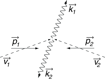
Figure 1: Kinematics for the process $e^{-}e^{+}\rightarrow 2\gamma$ in the center of momentum frame. Note that the velocities of the incident beams are not in general equal and opposite due to the difference in directions of the group velocity $\vec{v}$ and the momentum $\vec{p}$.

To obtain the physical cross section, the conventional steps are now followed. The electron and positron spins are averaged over and the final state photon polarizations are summed over. The momentum of the electron beam is chosen to point in the 3-direction for simplicity. The incident flux factor is divided out and the final state photon phase space is included. As a final step, the azimuthal angle is integrated over to simplify the expression.

The resulting cross section becomes

$${d\sigma\over d\cos{\theta}}=\int_{0}^{2\pi}d\phi{d\sigma\over d\Omega}=\left({d\sigma\over d\cos{\theta}}\right)_{QED}[1+\Delta]\quad,$$ (28)

where the first factor represents the conventional QED cross section and the Lorentz-violating correction $\Delta$ is given by

$$\Delta=c_{00}+c_{33}-2{\cos^{2}{\theta}\over 1+\cos^{2}{\theta}}(c_{11}+c_{22}-2c_{33})\quad.$$ (29)

The correction consists of a piece that is an overall scaling of the cross section and another part that modifies the angular dependence. Note that the cross section is now explicitly time-dependent since the $c_{ij}$ components change as the Earth rotates. This occurs because the 3-direction points along the electron beam momentum that rotates along with the earth.

To understand the time dependence, it is useful to transform to a fixed basis $(\hat{X},\hat{Y},\hat{Z})$ with the $\hat{Z}$-direction along the axis of the earth and the other two directions fixed with respect to the background stars. [9] The components of $c$ with respect to this basis are fixed so the time-dependence can be explicitly extracted from the cross section. For example, the term $c_{33}$ expressed in terms of the fixed basis is

$$c_{33}= c_{ZZ}+{\textstyle{1\over 2}}(c_{XX}+c_{YY}-2c_{ZZ})\sin^{2}{\chi}$$ (30)

$$+{\textstyle{1\over 2}}(c_{YZ}+c_{ZY})\sin{2\chi}\sin{\Omega t}+{\textstyle{1\over 2}}(c_{XZ}+c_{ZX})\sin{2\chi}\cos{\Omega t}$$

$$+{\textstyle{1\over 2}}(c_{XY}+c_{YX})\sin^{2}{\chi}\sin{2\Omega t}+{\textstyle{1\over 2}}(c_{XX}-c_{YY})\sin^{2}{\chi}\cos{2\Omega t}.$$

In this expression, $\chi$ is the angle between $\hat{p}$ and $\hat{Z}$, and $\Omega$ is the sidereal rotation frequency of the earth. Note that there are three components to the time dependence: a time-independent factor, a piece that varies with period $T=2\pi/\Omega$ and another piece with period $T=\pi/\Omega$. The conventionally measured cross section gives the time integrated constant part as the times are effectively averaged.

6 Summary

A framework has been developed for calculation of cross sections and decay rates within the context of the Lorentz-violating standard model extension. The modified Feynman rules and kinematical factors have been deduced. It was found that it is most convenient to perform the analysis in a single frame due to complications arising from the frame-dependent field redefinition. The cross section for $e^{-}e^{+}\rightarrow 2\gamma$ was calculated explicitly using the framework developed. It was found that the modifications to the conventional cross section are dependent on sidereal time due to the rotation of the earth. This time dependence is a qualitatively new feature of cross sections in the presence of Lorentz violation.

References

References

- [1] V.A. Kostelecký and S. Samuel, Phys. Rev. D 39, 683 (1989); ibid. 40, 1886 (1989); Phys. Rev. Lett. 63, 224 (1989); ibid. 66, 1811 (1991); V.A. Kostelecký and R. Potting, Nucl. Phys. B 359, 545 (1991); Phys. Lett. B 381, 89 (1996); Phys. Rev. D 63, 046007 (2001); V.A. Kostelecký, M. Perry, and R. Potting, Phys. Rev. Lett. 84, 4541 (2000).
- [2] S. Carroll, et al., Phys. Rev. Lett. 87, 141601 (2001); Also see, for example, C.D. Lane, these proceedings.
- [3] D. Colladay and V.A. Kostelecký, Phys. Rev. D 55, 6760 (1997); Phys. Rev. D 58, 116002 (1998).
- [4] See these proceedings for many examples.
- [5] D. Colladay and V.A. Kostelecký, Phys. Lett. B 511, 209 (2001).
- [6] S.M. Carroll, G.B. Field, and R. Jackiw, Phys. Rev. D 41, 1231 (1990); V.A. Kostelecký and M. Mewes, preprint IUHET 438, July 2001; M. Mewes, these proceedings.
- [7] R. Bluhm et al., Phys. Rev. Lett. 79, 1432 (1997); Phys. Rev. D 57, 3932 (1998).
- [8] V.A. Kostelecký and R. Lehnert, Phys. Rev. D 63, 065008 (2001).
- [9] V.A. Kostelecký, and C.D. Lane, Phys. Rev. D 60, 116010 (1999); J. Math. Phys. 40, 6245 (1999).