CERN-TH/2001-371
TSL/ISV-2001-0258
January, 2002

The thrust and heavy-jet mass distributions
in the two-jet region

Einan Gardi⁽¹⁾  and  Johan Rathsman^(1,2)

⁽¹⁾ TH Division, CERN, CH-1211 Geneva 23, Switzerland

⁽²⁾ High Energy Physics, Uppsala University, Box 535, S-751 21 Uppsala, Sweden

Abstract: Dressed Gluon Exponentiation (DGE) is used to calculate the thrust and the heavy-jet mass distributions in $e^{+}e^{-}$ annihilation in the two-jet region. We perform a detailed analysis of power corrections, taking care of the effect of hadron masses on the measured observables. In DGE the Sudakov exponent is calculated in a renormalization-scale invariant way using renormalon resummation. Neglecting the correlation between the hemispheres in the two-jet region, we express the thrust and the heavy-jet mass distributions in terms of the single-jet mass distribution. This leads to a simple description of the hadronization corrections to both distributions in terms of a single shape function, whose general properties are deduced from renormalon ambiguities. Matching the resummed result with the available next-to-leading order calculation, we get a good description of the thrust distribution in a wide range, whereas the description of the heavy-jet mass distribution, which is more sensitive to the approximation of the phase space, is restricted to the range $\rho_{H}<1/6$. This significantly limits the possibility to determine $\alpha_{s}$ from this observable. However, fixing $\alpha_{s}$ by the thrust analysis, we show that the power corrections for the two observables are in good agreement.

1 Introduction

Hadronic jets from the fragmentation of high-energy partons is one of the most spectacular phenomena in particle physics. It also provides evidence for the partonic nature of hadrons: observables such as event-shape distributions can be calculated perturbatively in terms of quarks and gluons and compared with hadronic final state measurements [1]. At the same time, these observables are directly sensitive to the hadronization process, providing an opportunity to learn more about the confinement mechanism from experiment.

The LEP experiments and their high quality data have prompted much theoretical progress in the understanding of QCD radiation and in the development of appropriate tools. This includes Sudakov resummation [2]–[6], renormalon resummation [7]–[9] and parametrization of power corrections [7]–[24].

Our goal is to extract from QCD quantitative predictions for event-shape distributions in the two-jet region. The precise LEP data provide a strong motivation for such an effort: it can be used for precision measurements of $\alpha_{s}$, but most importantly to test and improve our understanding of the QCD dynamics. An essential requirement is to understand how perturbative QCD can provide a reliable starting point for the calculation of event-shape distributions. Only then can one address the question of non-perturbative corrections.

The region where perturbation theory applies is limited from both ends. The multijet region is in principle accessible by going to ever higher orders. In practice, however, these calculations soon become difficult. On the other hand, the cross section is large only in the two-jet region, where it is determined by soft and collinear radiation. Close enough to the two-jet limit, the relevant scale for gluon emission becomes of order of the QCD scale $\Lambda$, and the problem becomes essentially non-perturbative.

In the two-jet region one must take into account the two immediate consequences of the restricted phase space, namely multiple emission and low scales. Even a qualitative description of the distribution ${d\sigma/{dy}\,(Q,y)}$, where $Q$ is the centre-of-mass energy and $y$ is an event-shape variable that vanishes in the two-jet limit, requires all-order resummation of Sudakov logs $L\equiv\ln 1/y$. Such resummation guarantees the vanishing of the cross section at $y=0$, whereas any fixed-order calculation diverges in this limit.

Sudakov logs can be resummed thanks to the factorization property of QCD matrix elements. The minimal resummation required for quantitative predictions is one where the Sudakov exponent is calculated to next-to-leading logarithmic (NLL) accuracy [2]–[6]. In NLL resummation the exponent includes terms of the form $\alpha_{s}^{n}L^{n+1}$ and $\alpha_{s}^{n}L^{n}$ for any $n$, while terms of the form $\alpha_{s}^{n}L^{m}$ with $m<n$ are neglected. The NLL exponentiation formula has become the standard tool for data analysis in recent years. Superficially this resummation applies for arbitrarily small $y$. However, due to the running of the coupling it actually applies only for $yQ\gg\Lambda$. In particular, when $yQ\sim\Lambda$ not only does the perturbative approximation break down completely, but also power corrections of arbitrary power $\sim\left(\Lambda/(yQ)\right)^{n}$ become important.

Since the distribution peak is located at $yQ\mathrel{\raise 1.29167pt\hbox{$>$\kern-7.5pt\lower 4.30554pt\hbox{$\sim$}}}\Lambda$, Sudakov resummation with a fixed logarithmic accuracy, such as NLL, is insufficient there. The low scales involved manifest themselves in renormalons: large perturbative coefficients that increase factorially at large orders. These large coefficients enhance the subleading logs $\alpha_{s}^{n}L^{m}$ with $m<n$, disrupting the dominance of the leading logs. Estimates [9] of the contribution of subleading logs, which are neglected in the standard NLL resummation, to the thrust ($T$) distribution at $(1-T)Q\gg\Lambda$ is of the order of $20\%$ at $Q={M_{\rm Z}}$.

In Dressed Gluon Exponentiation (DGE) [9, 25] the Sudakov exponent is calculated, starting with an off-shell gluon emission. Following the spirit of BLM [26]–[29] and [22, 7], the actual gluon virtuality is used as the scale of the running coupling. Through the integral over the coupling DGE resums the renormalon contribution (in the large $\beta_{0}$ limit) to the Sudakov exponent, and thus it takes into account the factorially enhanced subleading logs to any logarithmic accuracy. As a consequence, the calculated exponent is renormalization-scale invariant.

The calculation of the exponent by DGE makes the simplifying assumption that gluons are emitted independently. While reproducing the exact result to NLL accuracy [2, 3], this simplification amounts to approximations in both the phase space and the matrix elements beyond this accuracy. Nevertheless, since the two sources of large coefficients, Sudakov logs and renormalons, are accounted for, we consider DGE a reliable starting point for the analysis of the distribution in the range $yQ\mathrel{\raise 1.29167pt\hbox{$>$\kern-7.5pt\lower 4.30554pt\hbox{$\sim$}}}\Lambda$. Eventually, the dominance of the corrections we resum should be tested when the complete next-to-next-to-leading logarithmic (NNLL) and next-to-next-to-leading order (NNLO) corrections becomes available.

Physically it is clear that non-perturbative corrections due to soft gluon emission are important in the two-jet region. Technically, the DGE calculation gives a clear indication for the presence of power-suppressed corrections: the resummation of infrared renormalons is ambiguous at power accuracy. Consistency of the full cross section implies the existence of genuine power corrections of the same form. As in [11, 12] and [19]–[23] we will assume that these power corrections dominate over power corrections that have no trace in the perturbative calculation. This has far-reaching implications concerning the functional form of the non-perturbative correction. The leading corrections can be written as a convolution of the perturbative result with a shape function of a single variable $yQ$, as suggested by Korchemsky and Sterman [13]–[18], [9]. The simplest approximation to the shape function amounts to a shift of the perturbative distribution, in accordance with [14, 23]. Based on the renormalon ambiguity (in the large $\beta_{0}$ limit) only power corrections corresponding to odd central moments of the shape function are present. This gives, on the one hand, an explanation for the success of shift-based fits and, on the other hand, an opportunity to test the renormalon dominance assumption by fitting the data and extracting higher moments.

The DGE method has been the basis of our analysis of the thrust distribution in [9]. The comparison with experimental data was encouraging in several respects: first, good fits were obtained in a wide range of energies and thrust values. These fits were quite stable under a variation of different parameters, such as the cuts on the fitting range in thrust. In addition, the value of $\alpha_{s}$ and the non-perturbative parameter were consistent between the shape-function- and the shift-based fits. Moreover, these values were also consistent with those obtained by fitting the average thrust using renormalon resummation [7]. Such consistency, which is a crucial test of whether the approximation used is satisfactory, is not achieved [31] in standard NLL fits where renormalons are not resummed.

One aspect that certainly deserves attention is the fact that the best fit value of $\alpha_{s}$ obtained in [9, 7], $\alpha_{s}^{\hbox{$\overline{\hbox{\tiny MS}}\,$}}({M_{\rm Z}})=0.110$, is significantly lower than the world average [32] value $\alpha_{s}^{\hbox{$\overline{\hbox{\tiny MS}}\,$}}({M_{\rm Z}})=0.1172\pm 0.0020$. The experimental uncertainty is very small and the sources of theoretical uncertainty investigated in [9] hardly sum up to $5\%$. The latter uncertainty is dominated by non-logarithmic corrections at NNLO, which should become available in the foreseeable future.

It is of great interest to extend the application of DGE to more event-shape distributions. The main motivation is to test and improve our understanding of various perturbative and non-perturbative questions. In particular, it is interesting to investigate the relations between non-perturbative corrections to different observables. The idea of a “universal” (observable-independent) origin of the leading power corrections to various event-shape observables has been the subject of much theoretical and phenomenological activity in the past few years. Universal power corrections were suggested both within the infrared finite coupling approach [19]–[21], and in the shape-function approach [17]. In either case, the observable independence of the power corrections involves additional assumptions.

Probably the most relevant pair of variables to be compared in this respect are the thrust and the heavy-jet mass. For completeness we recall their definitions here, together with some other, closely related, jet mass variables:

Thrust $$T\equiv\max_{\vec{n}_{T}}\frac{\sum_{i}|\vec{p}_{i}\cdot\vec{n}_{T}|}{\sum_{i}|\vec{p}_{i}|}$$ (1)

Single-jet mass $$\rho_{m}\equiv\frac{\left(\sum_{i\in{\rm H}_{m}}p_{i}\right)^{2}}{\left(\sum_{i}p_{i}\right)^{2}}=\frac{\left(\sum_{i\in{\rm H}_{m}}p_{i}\right)^{2}}{Q^{2}}$$ (2)

Heavy-jet mass $$\rho_{H}\equiv\max(\rho_{1},\rho_{2})$$ (3)

Light-jet mass $$\rho_{L}\equiv\min(\rho_{1},\rho_{2}).$$ (4)

Here the index $i$ runs over all the particles and $m=1,2$ represents the two hemispheres ${\rm H}_{m}$ defined by the thrust axis $\vec{n}_{T}$.

There are several useful relations between these observables, which follows from their definition: the single-jet mass is the average of the heavy and the light,

$$\frac{1}{\sigma}\frac{d\sigma}{d\rho}=\frac{1}{2}\left[\frac{1}{\sigma}\frac{d\sigma}{d\rho_{H}}+\frac{1}{\sigma}\frac{d\sigma}{d\rho_{L}}\right]\;.$$ (5)

In the two-jet region $t\equiv 1-T$ equals, up to corrections suppressed by $t$, the sum of the two jet masses [3]

$$t\simeq\rho_{H}+\rho_{L}\;.$$ (6)

To leading order in $\alpha_{s}$ this relation is exact and, since the light-jet mass vanishes at this order, it follows that

$$\frac{1}{\sigma}\frac{d\sigma}{dt}=\frac{1}{\sigma}\frac{d\sigma}{d\rho_{H}}=2\frac{1}{\sigma}\frac{d\sigma}{d\rho}\quad\quad\left({\cal O}(\alpha_{s})\right).$$ (7)

In the approximation of independent emission used here, both the thrust and heavy-jet mass distributions can be expressed in terms of the single-jet mass distribution [3]. This implies that a single shape function [17] can be used to parametrize the non-perturbative corrections in both cases. On the other hand, fits based on the NLL resummation formula and a shift for the two distributions yield different values of $\alpha_{s}$, along with a different magnitude for the power correction (the shift) [31]. While a fair comparison of the power corrections must assume a common value of $\alpha_{s}$, such a fit does not improve the agreement between the power correction parameters. We will see below (Fig. 9) that fitting the heavy-jet mass distribution by shifting the NLL distribution, as in [31], but fixing the value of $\alpha_{s}$ based on the thrust fit, the power correction of the heavy-jet mass is much smaller ($\sim 50\%$) than expected based on the thrust fit.

Since the relation between the power corrections to the heavy-jet mass and those to the thrust follows from the definition of these variables, the discrepancy between the power corrections must be interpreted as a sign that the approximations made in the calculation are too crude. Based on [9, 7], it is quite clear that one reason for this discrepancy is the fact that renormalon contributions were neglected. We will verify this assertion in what follows.

In [17], the relation between the non-perturbative corrections to the two distributions was explained in terms of a strong correlation between the two hemispheres due to non-perturbative soft gluon emission at large angles. It was shown that introducing a positive correlation through a two-hemisphere shape function, the heavy-jet mass and the thrust (as well as the $C$-parameter) can be fitted. However, such a correlation, if important, should appear first at the perturbative level. Since the resummation formulae implicitly assume independent emission, and thus no correlation, we would rather not introduce such a correlation on the non-perturbative level. We shall assume here that in the two-jet region the jet masses are uncorrelated also on the non-perturbative level, and confront this assumption with the data.

Another important issue in the comparison of power corrections to the thrust and the heavy-jet mass is the dependence of the distribution on the hadron masses [24]. The perturbative calculation is based on massless partons, whereas the measured observable is based on massive hadrons. It is clear that the spectrum of hadrons has some effect on the distribution. In general at high enough $Q$ and $y$, the details of the spectrum do not matter. Instead, some generic characteristics of hadronization dominate, and a small set of non-perturbative parameters controlling power corrections is sufficient. However, the comparison of the thrust and the heavy-jet mass is problematic since the thrust is (conventionally) defined in terms of the three-momenta whereas the heavy-jet mass in terms of the four-momenta. This implies that the two observables will exhibit different sensitivity to the masses of the measured particles. Ways to overcome this difficulty by appropriate modifications of the definitions (which coincide with the standard ones in the massless limit) were suggested in [24]. We will see that choosing a common modification of the definition (hadron mass scheme) for the two observables is indeed crucial for a meaningful comparison of the power corrections.

The outline of this paper is as follows. We start in section 2 by recalling the perturbative calculation of the thrust and the heavy jet mass distribution using DGE. We then discuss the limitations of the approximation at hand, and, finally, we present our assumptions concerning hadronization corrections. Section 3 summarizes the data analysis. We begin by performing separate fits to the thrust and the heavy-jet mass distributions and then study the consistency between the two. Section 4 contains our conclusions.

2 Assumptions and calculation

In this section we present the calculation of the distributions, emphasizing the main assumptions involved. In section 2.1 we calculate the jet mass distribution from a single dressed gluon (SDG). In section 2.2, we exponentiate the SDG cross section arriving at the DGE formula for the single-jet mass distribution. This distribution is then used to express the thrust and the heavy-jet mass distributions. In section 2.3 we discuss the limitations of the considered approximation. Finally, in section 2.4 we present our approach concerning the parametrization of hadronization corrections and the way we deal with hadron mass effects.

2.1 Single Dressed Gluon cross section

We begin by calculating the differential cross section for a single gluon emission. The calculation is performed with an off-shell gluon $k^{2}=m^{2}\geq 0$ in order to provide the basis for renormalon resummation [22, 27, 28, 7, 8, 9]. Contrary to [8, 9], which used the full matrix element and identified the log-enhanced terms prior to the integration over the gluon virtuality, we will follow the approximation suggested in [25], which allows to isolate the relevant terms right at the beginning.

By performing the calculation with an off-shell gluon we will effectively be integrating inclusively over the decay products of the gluon. Based on the definitions of the variables (1) – (4) such a calculation yields the exact result when the partons that the gluon decays into are confined to a single hemisphere, but not so when these partons end up in different hemispheres. Therefore, our result should be considered as an approximation even in the large $\beta_{0}$ (large $N_{f}$) limit [38]. There are strong indications that this inclusive approximation is good in the case of the thrust [22, 7, 8, 9]. We will return to discuss this point in the section 2.3.

Let us denote the final momenta of the two quarks by $p$ and $\bar{p}$, where $p^{2}=\bar{p}^{2}=0$. Sudakov logs are associated with the singularity of the quark propagator prior to the emission, $(\mbox{$p$\raisebox{0.43057pt}{$/$}}+\mbox{$k$\raisebox{0.43057pt}{$/$}})/(p+k)^{2}$. Concentrating in the two-jet region, we will neglect non-logarithmic terms in the cross section. This is equivalent to neglecting non-singular terms in the matrix element [25]. It is convenient to use the light-cone axial gauge [25] where, in the approximation considered, the gluon effectively decouples from one of the quarks.

Assuming that the gluon is in the hemisphere of the quark $p$, it is $\bar{p}$ that sets the thrust axis (we will calculate the cross section only in this half of phase space and account for the other half by an overall factor of 2). We define the light-cone coordinates such that $p=(p_{+},0,0)$ and $\bar{p}=(0,\bar{p}_{-},0)$, and use the light-cone gauge where $A_{+}=0$. In this gauge the gluon coupling to the $\bar{p}$ quark is suppressed, so it is enough to consider the diagram where the gluon is emitted from $p$. The gluon propagator is given by

$$d_{\mu\nu}=-g_{\mu\nu}+\frac{k_{\mu}\bar{p}_{\nu}+\bar{p}_{\mu}k_{\nu}}{k\bar{p}}.$$ (8)

The cross section in the centre-of-mass frame is

$$\sigma=\frac{e^{4}N_{c}\sum_{q}e_{q}^{2}}{2Q^{2}}\int\frac{d^{4}p\,d^{4}\bar{{p}}}{(2\pi)^{6}}\,\delta\left(p^{2}\right)\,\delta\left(\bar{p}^{2}\right)\frac{d^{4}k}{(2\pi)^{3}}\,\delta\left(k^{2}-m^{2}\right)(2\pi)^{4}\delta^{4}(q-p-\bar{p}-k)\,\frac{H_{\rho\sigma}\,L^{\rho\sigma}}{Q^{4}}.$$

The leptonic tensor $L^{\rho\sigma}=\frac{1}{4}{\rm Tr}\left\{\mbox{$q$\raisebox{0.43057pt}{$/$}}_{1}\gamma^{\rho}\mbox{$q$\raisebox{0.43057pt}{$/$}}_{2}\gamma^{\sigma}\right\}$ can be replaced by $\frac{1}{3}Q^{2}g^{\rho\sigma}$. To calculate the hadronic tensor $g_{\rho\sigma}\,H^{\rho\sigma}=\sum_{\mbox{\rm{\hbox{\tiny spins}}}}{\cal{M}}{\cal{M}}^{\dagger}$ we write the amplitude

$${\cal M}=g_{s}\,t^{a}\,{\epsilon^{\lambda}_{\mu}}^{*}\,\frac{1}{(k+p)^{2}}\,\bar{u}^{(s)}(p)\gamma^{\mu}(\mbox{$p$\raisebox{0.43057pt}{$/$}}+\mbox{$k$\raisebox{0.43057pt}{$/$}})\gamma^{\rho}u^{(\bar{s})}({\bar{p}})$$ (9)

where $t^{a}$ is a colour matrix and ${\epsilon^{\lambda}_{\mu}}^{*}$ is the gluon polarization vector. The squared matrix element summed over the gluon and quark spins is then given by

$$\sum_{\mbox{\rm{\hbox{\tiny spins}}}}{\cal{M}}{\cal{M}}^{\dagger}=\frac{C_{F}g_{s}^{2}}{(k+p)^{4}}\,g_{\rho\sigma}\,d_{\mu\nu}{\rm Tr}\left\{(\mbox{$p$\raisebox{0.43057pt}{$/$}}+\mbox{$k$\raisebox{0.43057pt}{$/$}})\gamma^{\nu}\mbox{$p$\raisebox{0.43057pt}{$/$}}\gamma^{\mu}(\mbox{$p$\raisebox{0.43057pt}{$/$}}+\mbox{$k$\raisebox{0.43057pt}{$/$}})\gamma^{\rho}\mbox{$\bar{p}$\raisebox{0.43057pt}{$/$}}\gamma^{\sigma}\right\}$$ (10)

where $\sum_{s}u^{(s)}(p)\bar{u}^{(s)}(p)$ was replaced by $p$$/$, and $\sum_{\lambda}{\epsilon_{\nu}^{\lambda}}^{*}\epsilon_{\mu}^{\lambda}$ by $d_{\mu\nu}$. Introducing the Sudakov decomposition of $k=(k_{+},k_{-},k_{\perp})=\beta p+\alpha\bar{p}+k_{\perp}$, and defining the following dimensionless parameters

$$\beta = k_{+}/p_{+}=2k\bar{p}/2p\bar{p}$$

$$\alpha = k_{-}/\bar{p}_{-}=2kp/2p\bar{p}$$ (11)

$$\gamma \equiv k_{\perp}^{2}/2p\bar{p}$$

$$\lambda = m^{2}/2p\bar{p}=(2k_{+}k_{-}-k_{\perp}^{2})/2p\bar{p}=\alpha\beta-\gamma,$$

the propagator is proportional to $1/(\alpha+\lambda)^{2}$. As observed in [25], to calculate the log-enhanced cross section, it is sufficient to take into account the singular terms in the matrix element, corresponding to the situation where both $\alpha$ and $\lambda$ are small (with no specific hierarchy between them). From the condition $\alpha\beta=\gamma+\lambda$ it follows that the transverse momentum fraction $\gamma$ is also small (at least with respect to $\beta$) while $\beta$ can be either large (the collinear limit) or small (the soft limit). In these variables

$$\sum_{\mbox{\rm{\hbox{\tiny spins}}}}{\cal{M}}{\cal{M}}^{\dagger}=8C_{F}g_{s}^{2}\,\left[\frac{-\lambda}{({\alpha+\lambda})^{2}}\,(1+\beta)+\frac{1}{\alpha+\lambda}\,\frac{\beta^{2}+2\beta+2}{\beta}\right].$$ (12)

The cross section is therefore,

$$\sigma/\sigma_{0}=\frac{C_{F}\alpha_{s}}{\pi}\int\frac{d\alpha\,d\beta\,d\lambda\,\delta(\lambda-\epsilon(1+\beta))}{(1+\beta)^{3}}\,\left[\frac{-\lambda}{({\alpha+\lambda})^{2}}\,(1+\beta)+\frac{1}{\alpha+\lambda}\,\frac{\beta^{2}+2\beta+2}{\beta}\right]$$ (13)

where $\sigma_{0}={N_{c}(\sum_{q}e_{q}^{2})\,4\pi\alpha^{2}}/{(3Q^{2})}$ and the $\delta$ function guarantees that the integration is performed for a fixed $\epsilon\equiv m^{2}/Q^{2}$ and $Q^{2}$. The integrand has the interpretation of a generalized, off-shell gluon splitting function [25].

We are now ready to calculate the differential cross section for the jet mass distribution. The hemisphere of the quark $p$ to which the gluon is emitted is the heavy one, $m_{H}^{2}=(p+k)^{2}/Q^{2}$, whereas the other has zero mass, $m_{L}^{2}=0$. The relation between $\rho_{H}={m_{H}^{2}}/{Q^{2}}$ and the Sudakov variables (2.1) is simply

$$\rho_{H}=\frac{(p+k)^{2}}{Q^{2}}=\frac{2pk+k^{2}}{Q^{2}}=\frac{(\alpha+\lambda)\,2p\bar{p}}{Q^{2}}=\frac{\alpha+\lambda}{1+\alpha+\beta+\lambda}\simeq\frac{\alpha+\lambda}{1+\beta}.$$ (14)

Note that also $t=1-T=(m_{H}^{2}+m_{L}^{2})/Q^{2}=\rho_{H}$.

Changing variables in (13) we get the following result for the single off-shell gluon differential cross section

$$\frac{1}{\sigma}\frac{d\sigma}{d\rho_{H}}\,=\,\frac{C_{F}\alpha_{s}}{\pi}\,\int\,\frac{d\beta}{(1+\beta)^{2}}\,\left[-\frac{\epsilon}{\rho_{H}^{2}}+\frac{1}{\rho_{H}}\,\frac{\beta^{2}+2\beta+2}{\beta\,(1+\beta)}\right].$$ (15)

Next, in the integration over $\beta$, it is the limit of vanishing transverse momentum $\alpha\beta=\lambda$ that generates the log-enhanced terms [25]. We therefore integrate over $\beta$ and substitute the limit $\beta=\epsilon/(\rho_{H}-\epsilon)$. The result is

$$\frac{1}{\sigma}\frac{d\sigma}{d\rho_{H}}\,=\,\frac{C_{F}\alpha_{s}}{\pi}\,\left[\frac{2}{\rho}_{H}\,\ln\frac{\rho_{H}}{\epsilon}-\frac{3}{2}\frac{1}{\rho}_{H}+\frac{\epsilon}{\rho_{H}^{2}}+\frac{1}{2}\frac{\epsilon^{2}}{\rho_{H}^{3}}\right].$$ (16)

Using the gluon bremsstrahlung effective charge [33] $\alpha_{s}\longrightarrow\bar{\alpha}_{s}$ is sufficient to guarantee that the singular terms in the splitting functions are exact. This way the renormalization scheme is not arbitrary: there is a unique effective charge that generates correctly subleading terms. Provided one also uses the two-loop renormalization group equation, the calculation of the thrust and the heavy-jet mass distributions will be exact [33, 9] to NLL accuracy.

We now replace $\bar{\alpha}_{s}$ by an integral over the time-like discontinuity of the coupling [22, 27, 28]. In this way we take into account the relevant physical scale for the gluon emission $k^{2}=\epsilon Q^{2}$. Defining $\bar{A}(k^{2})\equiv\beta_{0}\bar{\alpha}_{s}(k^{2})/\pi$, we will use here the scheme invariant Borel representation [35]–[37],

$$\bar{A}(k^{2})=\int_{0}^{\infty}d{u}\,\exp\left({-{u}\ln k^{2}/\bar{\Lambda}^{2}}\right)\bar{A}_{B}({u}),$$ (17)

where $\bar{A}_{B}(u)=1$ for the one-loop coupling, provided $\bar{\Lambda}$ is defined appropriately. The integrated time-like discontinuity is [34, 22]

$$\bar{A}_{\hbox{\tiny eff}}(Q^{2})=\int_{0}^{\infty}d{u}\,\exp\left(-{{u}\ln Q^{2}/\bar{\Lambda}^{2}}\right)\,\frac{\sin\pi{u}}{\pi{u}}\,\bar{A}_{B}({u}).$$ (18)

After integration by parts the single dressed gluon cross section is

$$\left.\frac{1}{\sigma}\frac{d\sigma}{d\rho_{H}}(Q^{2},\rho_{H})\right|_{\hbox{\tiny SDG}}=\frac{C_{F}}{\beta_{0}}\int_{\rho_{H}^{2}}^{\rho_{H}}\frac{d\epsilon}{\epsilon}\,\bar{A}_{\hbox{\tiny eff}}(\epsilon Q^{2})\left[\frac{2}{\rho_{H}}-\frac{\epsilon}{\rho_{H}^{2}}-\frac{\epsilon^{2}}{\rho_{H}^{3}}\right].$$ (19)

Here, the upper integration limit is determined from the condition that $\alpha$ is positive. Along the zero transverse momentum boundary of phase space, the limit is $\alpha=(\rho_{H}-\epsilon)(1+\beta)=0$. In this situation both $k_{\perp}^{2}$ and $k_{-}$ vanish, so the gluon is exactly collinear. The lower integration limit is determined from the requirement that $\beta>\alpha$ (otherwise the gluon belongs to the $\bar{p}$ hemisphere). Along the zero transverse momentum boundary $\alpha\beta=\lambda$, this condition translates into $\beta>\sqrt{\lambda}$. It follows that the lower integration limit is $\epsilon=\rho_{H}^{2}$. This limit corresponds to large-angle, soft emission.

To obtain the single-jet mass distribution we have to average over the heavy and the light hemispheres. But since the light-jet mass cross section starts at two gluon emission (order $\alpha_{s}^{2}$) this amounts, according to (7), to dividing the heavy jet mass cross section by 2,

$$\left.\frac{1}{\sigma}\frac{d\sigma}{d\rho}(Q^{2},\rho)\right|_{\hbox{\tiny SDG}}=\frac{C_{F}}{2\beta_{0}}\int_{\rho^{2}}^{\rho}\frac{d\epsilon}{\epsilon}\,\bar{A}_{\hbox{\tiny eff}}(\epsilon Q^{2})\left[\frac{2}{\rho}-\frac{\epsilon}{\rho^{2}}-\frac{\epsilon^{2}}{\rho^{3}}\right].$$ (20)

Substituting (18) into (20) and performing the integral over $\epsilon$ yields the Borel representation of the logarithmically enhanced SDG cross section,

$$\left.\frac{1}{\sigma}\frac{d\sigma}{d\rho}(Q^{2},\rho)\right|_{\hbox{\tiny SDG}}=\frac{C_{F}}{2\beta_{0}}\int_{0}^{\infty}\,du\,B_{\hbox{\tiny SDG}}(u,\rho)\,\exp\left(-{{u}\ln Q^{2}/\bar{\Lambda}^{2}}\right)\,\frac{\sin\pi u}{\pi u}\bar{A}_{B}(u)$$ (21)

with the following Borel function [9]

$$B_{\hbox{\tiny SDG}}(u,\rho)=\frac{1}{\rho}\left[\frac{2}{u}\exp\left(2u\ln\frac{1}{\rho}\right)-\left(\frac{2}{u}+\frac{1}{1-u}+\frac{1}{2-u}\right)\exp\left({u}\ln\frac{1}{\rho}\right)\right]\,.$$ (22)

This result was discussed in detail in [9]. Here we just recall that the sensitivity to soft gluon emission does not appear here through Borel singularities (which cancel out by the $\sin(\pi u)$ factor) but rather as convergence constraints on the Borel integration at $u\to\infty$.

2.2 Exponentiation

Assuming independent emission and additive contribution by each emission to the jet mass: $\rho=\sum_{k=1}^{n}\rho_{k}$, the multiple gluon phase space factorizes in Laplace space [3]. As in [9], the DGE cross section is obtained by exponentiating the SDG cross section, given by (21) and (22), under the Laplace transform. The Laplace transform $J(\nu,Q^{2})$ of the single-jet mass distribution is then given by

$$\ln J(\nu,Q^{2})=\int_{0}^{1}\left.\frac{1}{\sigma}\frac{d\sigma}{d\rho}(Q^{2},\rho)\right|_{\hbox{\tiny SDG}}\left(e^{-\nu\rho}-1\right)d\rho,$$ (23)

where the Laplace weight $e^{-\nu\rho}$ is associated with real emissions and $-1$ with virtual corrections. The corresponding Borel representation [9] is

$$\ln J(\nu,Q^{2})=\frac{C_{F}}{2\beta_{0}}\int_{0}^{\infty}\,du\,B(\nu,u)\,\exp\left(-{{u}\ln Q^{2}/\bar{\Lambda}^{2}}\right)\,\frac{\sin\pi u}{\pi u}\bar{A}_{B}(u)$$ (24)

with

$$B(\nu,u) = \int_{0}^{1}\frac{d\rho}{\rho}\left[\frac{2}{u}e^{2u\ln\frac{1}{\rho}}-\left(\frac{2}{u}+\frac{1}{1-u}+\frac{1}{2-u}\right)e^{u\ln\frac{1}{\rho}}\right]\,\left(e^{-\nu\rho}-1\right)$$

$$\simeq \frac{2}{u}\left[e^{2u\ln\nu}\Gamma(-2u)+\frac{1}{2u}\right]-\left(\frac{2}{u}+\frac{1}{1-u}+\frac{1}{2-u}\right)\left[e^{u\ln\nu}\Gamma(-u)+\frac{1}{u}\right],$$

where non-logarithmic terms have been neglected. Contrary to the SDG result (22), the DGE result has a rich renormalon structure, notably, it has singularities at half-integer values of $u$. These Borel singularities indicate power corrections. Note that the first term in (2.2), which has a double argument $2u$, corresponds to large-angle soft emission, whereas the second corresponds to collinear emission.

The single-jet mass distribution can be obtained by the inverse Laplace transform of (24):

$$\frac{1}{\sigma}\frac{d\sigma}{d\rho}(\rho,Q^{2})=\frac{d}{d\rho}\int_{C}\frac{d\nu}{2\pi i\nu}\,\exp\left\{\nu\rho+\ln J(\nu,Q^{2})\right\}\equiv\frac{d}{d\rho}R_{\rho}(Q^{2},\rho)\equiv j(\rho,Q^{2}),$$ (26)

where the contour $C$ goes from $-i\infty$ to $+i\infty$ to the right of all the singularities of the integrand. Using this distribution, the thrust $t=\rho_{1}+\rho_{2}$ distribution is

$$\frac{1}{\sigma}\frac{d\sigma}{dt}(t,Q^{2}) = \int d\rho_{1}d\rho_{2}\,j(\rho_{1},Q^{2})j(\rho_{2},Q^{2})\,\delta(\rho_{1}+\rho_{2}-t)$$

$$= \frac{d}{dt}\int_{C}\frac{d\nu}{2\pi i\nu}\,\exp\left\{\nu t+2\ln J(\nu,Q^{2})\right\}\equiv\frac{d}{dt}R_{t}(Q^{2},t),$$

whereas the heavy-jet mass $\rho_{H}=\rho_{1}\Theta(\rho_{1}-\rho_{2})+\rho_{2}\Theta(\rho_{2}-\rho_{1})$ distribution is

$$\!\!\!\!\!\!\!\!\!\!\!\!\!\!\!\!\!\!\!\!\!\!\!\!\frac{1}{\sigma}\frac{d\sigma}{d\rho_{H}}(\rho_{H},Q^{2})=$$ (28)

$$= \int d\rho_{1}d\rho_{2}\,j(\rho_{1},Q^{2})j(\rho_{2},Q^{2})\,\left[\delta(\rho_{1}-\rho_{H})\Theta(\rho_{1}-\rho_{2})+\delta(\rho_{2}-\rho_{H})\Theta(\rho_{2}-\rho_{1})\right]$$

$$= \frac{d}{d\rho_{H}}\,\int d\rho_{1}d\rho_{2}\,j(\rho_{1},Q^{2})j(\rho_{2},Q^{2})\,\Theta(\rho_{H}-\rho_{1})\Theta(\rho_{H}-\rho_{2})$$

$$= \!\!\!\!\frac{d}{d\rho_{H}}\,\left[\int_{C}\frac{d\nu}{2\pi i\nu}\,\exp\left\{\nu\rho_{H}+\ln J(\nu,Q^{2})\right\}\right]^{2}\equiv\frac{d}{d\rho_{H}}\,R_{\rho_{H}}(Q^{2},\rho_{H}).$$

Equations (2.2) and (28) are our final expressions (prior to matching with the NLO result) for the thrust and the heavy-jet mass distributions. Using $\ln J(\nu,Q^{2})$ in (24) with the two-loop gluon bremsstrahlung coupling, as we do below, these results are exact to NLL accuracy. However, they differ from [3] by large subleading logs which emerge from the integral over the running coupling. In order to understand how significant these additional terms are, it is useful [9] to rewrite $\ln J(\nu,Q^{2})$ as an asymptotic series in the coupling,

$$\ln J(\nu,Q^{2}) = \frac{C_{F}}{2\beta_{0}}\sum_{k=1}^{\infty}f_{k}\left(\xi\right)\bar{A}(Q^{2})^{k-2}\;,$$ (29)

where $\xi=\bar{A}(Q^{2})\ln\nu$. Truncation of this series amounts to a fixed logarithmic accuracy. The first two functions ($k=1,2$) coincide with the known leading and next-to-leading log functions, whereas $f_{k}$ for $k\geq 2$ are given by

$$\begin{array}[]{ll}f_{3}(\xi)={0.804}/{(1-\xi)}-{{2.32}/({1-2\xi})}\\ f_{4}(\xi)={0.779}/{({1-\xi})^{2}}-{{2.68}/{(1-2\xi)^{2}}}\\ f_{5}(\xi)={2.32}/{({1-\xi})^{3}}-{{5.00}/{(1-2\xi)^{3}}}\end{array}$$

where, for simplicity, we used a one-loop running coupling. At higher orders, these functions behave as

$$f_{k}(\xi) \sim (k-3)!\,\left[\frac{1}{(1-\xi)^{k-2}}-2.5\,\frac{1}{(1-2\xi)^{k-2}}\right].$$ (31)

The factorially increasing coefficients of $f_{k}(\xi)$ and the enhanced singularity at $\xi=1/2$ imply that a fixed logarithmic accuracy calculation holds only in a very restricted range in the $\bar{A}(Q^{2})$ and $L=\ln\nu\simeq\ln 1/\rho$ parameter space. Note that the contributions of two consequent terms in (29) are of the same order when $\bar{A}(Q^{2})\simeq(1-2\xi)/(k-2)$. At this order the perturbative expansion is exhausted (the minimal term is reached) and the correction is effectively power-like $\sim\,\bar{\Lambda}/(Q\rho)$. We assume below that the order of the minimal term is higher than NLL, so including higher orders in (29) improves the evaluation of $\ln J(\nu,Q^{2})$. Figures 2 and 3 in [9] show that near the distribution peak, and anywhere above it, $\rho>\rho({\rm peak})$, this is indeed the case. The fixed logarithmic accuracy calculation is justified if (29) converges well. For a fixed $\xi$ (any $\xi<1/2$) this holds if the coupling is very small $\bar{A}(Q^{2})\ll 1-2\xi$. However, for a given coupling, there is good convergence only for $\xi\ll 1/2$, i.e.

$${\rho}\gg\exp\left(-\frac{1}{2\bar{A}(Q^{2})}\right)=\frac{\bar{\Lambda}}{Q}.$$

This condition is not realized in the peak region at any relevant centre-of-mass energy. Consequently a fixed logarithmic accuracy is insufficient. The analysis of [9] showed, that in the case of the thrust, the contributions of NNLL and further subleading logs to $\ln J(\nu,Q^{2})$ at $Q={M_{\rm Z}}$ lead to a correction of $\sim 20\%$ for $\rho>\rho({\rm peak})$. Only when all the terms (up to the minimal term) in the series (29) are kept can one safely combine the perturbative calculation with the corresponding power corrections, eventually extending the applicability of the result to the peak region.

As explained in [9], when power accuracy is required, using (29) is cumbersome since the number of relevant terms varies as a function of $Q$ and $\rho$. To evaluate $\ln J(\nu,Q^{2})$ we therefore perform explicitly the Borel integral (24). The prescription we use to define the integral avoiding the renormalon singularities as well as the technique used for the analytic integration were explained in detail in [9].

To complete the perturbative calculation we need to match the resummed result with the exact NLO calculation, which includes non-logarithmic contributions. We do this using the so-called $\log R$ matching scheme [3]. This amounts to replacing the first two terms in the expansion of $\ln R(Q^{2},y)$ (where $y=t,\rho_{H}$) with the exact terms in the following way:

$$\left.\ln R(Q^{2},y)\right|_{\rm PT} = R_{1}(y)a(Q^{2})+\left(R_{2}(y)-\frac{1}{2}R_{1}(y)^{2}\right)a^{2}(Q^{2})$$

$$+\left.\ln R(Q^{2},y)\right|_{\rm DGE}-\left.\ln R(Q^{2},y)\right|_{\rm DGE}^{\rm NLO}\;.$$

Here $a=\alpha_{\overline{\mbox{\tiny MS}}}/\pi$, $R_{1}(y)$ and $R_{2}(y)$ denote the exact LO and NLO coefficients respectively, and $\left.\ln R(Q^{2},y)\right|_{\rm DGE}^{\rm NLO}$ is the expansion of the DGE resummed result to ${\cal O}(a^{2})$. For $R_{1}(y)$ we use the analytic results and for $R_{2}(y)$ we use formulae that parametrize the coefficients extracted numerically from EVENT2 [40]. Whereas the resummed DGE result is independent of the renormalization scale, the matched result has some scale dependence. Ignoring the renormalon contributions which are not logarithmically enhanced is justified a posteriori: in [9] the residual scale dependence was found to be very small for the thrust distribution ($\mathrel{\raise 1.29167pt\hbox{$<$\kern-7.5pt\lower 4.30554pt\hbox{$\sim$}}}1\%$ for $t<0.25$). We expect a similar dependence for the heavy-jet mass.

2.3 Limitations of the approximation used

The perturbative DGE result presented in the previous sections was the basis for the phenomenological analysis of the thrust distribution in [9] using (almost) the entire range in $t$. However, as will soon become clear, the range of applicability of the result for the heavy-jet mass is more restricted. To understand why, and eventually in what conditions a quantitative study of the heavy-jet mass can be performed, we will now return to some of the approximations made in the derivation and discuss their validity.

As any resummation, the DGE result captures specific features of the distribution, which show up as large corrections, neglecting other, sub-dominant features. To judge the quality of the approximation, we must know what we neglect. The first crucial comparison is, of course, with fixed-order results. Although the known fixed-order results (here LO and NLO) are taken into account by matching, their comparison with the resummed result is a valuable tool to identify the range of parameters where the approximation is valid and what it may miss at yet unavailable higher orders (NNLO and beyond).

The comparison of the ${\cal O}(\alpha_{s}^{2})$ term in the resummed result, expanded as

$$R(Q^{2},y)=1+R_{1}(y)a(Q^{2})+R_{2}(y)a^{2}(Q^{2})+\ldots,$$

with the exact NLO term calculated by EVENT2 [40], is shown in Fig. 1. The difference between the two increases for $y\gg y({\rm peak})$, particularly because of the non-logarithmic terms. The approximation for large values of the variable is much better in the case of the thrust compared to that of the heavy-jet mass. For example, the ratio between $dR_{2}^{\rm NLO}(t)/dt$ and $dR_{2}^{\rm DGE}(t)/dt$ is larger than $0.8$ for $t\leq 0.25$, whereas for the heavy-jet mass the corresponding ratio reaches $0.8$ already at $\rho_{H}=0.13$.

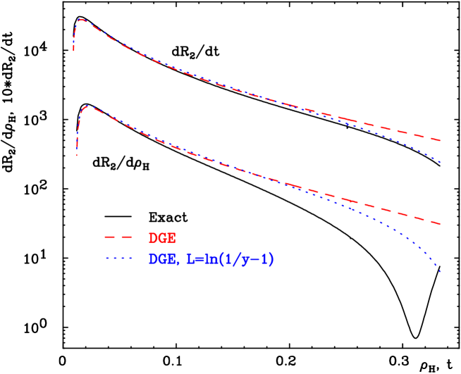
Figure 1: The NLO coefficient for the thrust (upper set of curves) and heavy-jet mass (lower set of curves) distributions obtained by expanding the DGE result (dashed and dotted line for the unmodified and modified log, respectively) compared to the exact result (solid line).

The figure also shows that for the thrust distribution a modification of the logarithm to $L=\ln(1/t-1)$, as suggested in [2], gives a better approximation for large $t$, whereas for intermediate $t$ ($\sim 0.1$) the approximation with a modified log is worse. In the case of the heavy-jet mass the effect of modifying the log is much smaller than the difference with the exact result. We conclude that in the latter case modifying the log cannot be considered as a reliable estimate of the uncertainty due to the missing non-logarithmic higher-order terms. We will explain why this is so, below.

Having based our exponentiation on the large $\beta_{0}$ limit, rather than on a fixed logarithmic accuracy, it is interesting to know which logs are computed exactly. As before, we categorize the logs as they appear in the exponent, $\ln J(\nu,Q^{2})$, consistently with [3]: leading logs are ${\cal O}(L^{n+1}\alpha_{s}^{n})$, NLL are ${\cal O}(L^{n}\alpha_{s}^{n})$, etc. In addition we must distinguish, at the level of the exponent, between terms that are leading in $\beta_{0}$ which are directly calculated (section 2.1) and terms that are subleading in $\beta_{0}$, e.g. ${\cal O}(C_{F}C_{A}L^{j}\alpha_{s}^{2})$, which are introduced through subleading terms in the splitting function or through the (two-loop) evolution of the coupling.

Terms that are leading in $\beta_{0}$ at the exponent would have been exact if not for non-inclusive contributions [38]. Such contributions first show up due to the emission of a soft gluon at large angle, that splits into a quark and an antiquark which end up in opposite hemispheres with respect to the thrust axis. The contribution of such an emission to the single jet mass $\ln J(\nu,Q^{2})$ is ${\cal O}(C_{F}\beta_{0}L\alpha_{s}^{2})$ i.e. NNLL. However, both the thrust and the heavy-jet mass distributions receive only a ${\cal O}(C_{F}\beta_{0}\alpha_{s}^{2})$ correction, i.e. $\rm N^{(3)}LL$. The reason is that in the latter case, contrary to the former, the observables and their inclusive approximations are of the same order – the order of the soft gluon momentum. Consequently, the difference between the integrated cross section and its inclusive approximation has support only in a small part of the phase space. The ${\cal O}(C_{F}\beta_{0}L\alpha_{s}^{2})$ term obtained from expanding the inclusive DGE result indeed coincides with the numerical value extracted from EVENT2. This was checked in the case of the thrust in [9] (see the appendix). We have now made a similar check for the heavy-jet mass.

Terms that are subleading in $\beta_{0}$ at the exponent are computed exactly to NLL accuracy for both the thrust (2.2) and the heavy-jet mass (28) distributions, thanks to the use of the two-loop renormalization group equation and the gluon bremsstrahlung effective charge. The latter includes the full non-Abelian contribution to the singular part of the splitting function [33, 9]. As in the Abelian case discussed above, the inclusive approximation has a price. The effect of a large-angle soft gluon that splits into two gluons which end up in opposite hemispheres is larger than in the Abelian case, because the second branching contains an additional soft singularity. Indeed, Dasgupta and Salam have shown [39] that the single-jet mass $\ln J(\nu,Q^{2})$ receives a ${\cal O}(C_{F}C_{A}L^{2}\alpha_{s}^{2})$ contribution, i.e. NLL, from such a configuration. As in the Abelian case, the corresponding contributions to the thrust and the heavy jet mass are suppressed, and appear at NNLL accuracy or beyond.

This discussion teaches us that the logarithmically enhanced terms are well under control for both the thrust and the heavy-jet mass distributions. The key to understanding the difference between these two cases, as reflected in Fig. 1 is the kinematic constraints on the jet masses, which manifest themselves primarily through non-logarithmic corrections.

When a hard gluon is emitted at a moderate angle (the heavy-jet mass is not very small) emission of further soft gluons is not controlled by the same matrix element. Also the phase space is drastically modified. This is not taken into account in our approximate calculation, where gluons are emitted off a quark–antiquark dipole. Moreover, we explicitly assumed in the derivation of (28) that the masses of the two hemispheres are independent. This assumption is consistent with the approximation of independent emission we employ in the two-jet region. However, it is clearly violated at larger $\rho_{H}$.

Figure 2: A contour plot of the doubly differential light and heavy-jet mass cross section based on 10 million events generated with Pythia at $Q={M_{\rm Z}}$ on the parton level, using only light quarks (uds). The contours spacing is based on a logarithmic scale: the lowest contour corresponds to two events and the others are spaced by a relative factor of 5. This illustrates the available phase space and, in particular, the constraints on $\rho_{L}$ for $\rho_{H}>1/6$.

Contrary to the approximation we use, in a realistic phase space, the two hemisphere masses are correlated. The easiest way to see this is to consider a slightly different definition of the jet masses, where the hemispheres are defined by minimizing the sum of the two jet masses $\rho_{\rm tot}\equiv\rho_{1}+\rho_{2}$. In this case it was shown [41] that the largest possible value of $\rho_{\rm tot}$ is $1/3$. This means that $\rho_{L}$ cannot exceed $\min\left\{\rho_{H},1/3-\rho_{H}\right\}$, which is always smaller than $1/6$. This constraint becomes quite stringent for large values of $\rho_{H}$. It manifests itself through a Sudakov form factor, which resums logarithms of the form $\ln(1/3-\rho_{H})$. These large perturbative corrections have nothing to do with the $\ln\rho_{H}$ terms that are resummed in the two-jet region.

Turning to the jet mass definition based on the thrust axis, the upper limit changes to $\rho_{1}+\rho_{2}\leq 1/2$, but the value of $\rho_{H}$ for which $\rho_{L}$ reaches its maximum is still $1/6$ (this value does not depend on the definition of the thrust axis, since at this point the distribution of particles is completely symmetric). The available phase space for $\rho_{L}$ as a function of $\rho_{H}$ is illustrated in Fig. 2. The figure shows the doubly differential cross section based on 10 million events generated with Pythia [42] for $Q={M_{\rm Z}}$ at the parton level.

Ignoring the kinematic constraints in the calculation, we definitely overestimate the cross section for $\rho_{H}>1/6$. Since the cross section for $\rho_{H}\geq 1/6$ is not negligible (it is of the order of $\sim 5\%$ at $Q={M_{\rm Z}}$), there is also an impact on the cross section below $1/6$. This explains the significant difference (Fig. 1) between the exact result and our approximation, as $\rho_{H}$ increases.

The kinematic constraint on the light-jet mass for $\rho_{H}>1/6$ is much more stringent than the general condition that the cross section vanishes at $\rho_{H}=1/2$. Whereas the former condition dictates the behaviour of the exact NLO coefficient in Fig. 1, it is the latter that is imposed by modifying the log from $\ln 1/\rho_{H}$ to $\ln(1/\rho_{H}-1)$. This explains why such a modification does not represent the actual effect of non-logarithmic terms at large $\rho_{H}$.

The reason why the effect on the thrust distribution is smaller also becomes clear: fixing $t$ at some moderate value does not put any stringent constraint on the light-jet mass, nor on any other shape variable. When $t$ reaches $1/3$ such constraints appear. However, since the cross section for $t>1/3$ is small (less than $1\%$ at $Q={M_{\rm Z}}$), the effect of ignoring the kinematic constraints on the cross section below $1/3$ is insignificant.

It should also be emphasized that the correlation between the hemisphere masses due to the restriction on their sum is negative. This should be contrasted with the dynamical correlation discussed in [17, 18], which is due to radiation from one hemisphere into the other (“non-inclusive” corrections [38]). This correlation is positive [8, 17, 18]. Recall that the non-inclusive correction at the NLO level was shown [8] (see table 2 there, and the explanation that follows) to be small in the case of the average thrust, but it increases for higher moments $\langle t^{2}\rangle$, $\langle t^{3}\rangle$, etc. Based on the definitions (1) and (3), both $t$ and $\rho_{H}$ are smaller in the full calculation than in the inclusive one, in configurations where a gluon decays into particles that end up in opposite hemispheres. Therefore, in the full, non-inclusive calculation the thrust distribution is somewhat flatter than in the inclusive one [8]. The same holds for the $\rho_{H}$ distribution. Thus, ignoring the radiation from one hemisphere into the other results in underestimating both the thrust and the heavy-jet mass distributions at large $t$ and $\rho_{H}$, respectively. On the other hand, Fig. 1 shows that ignoring the kinematic constraints as well as the radiation from one hemisphere into the other, results in overestimating the cross section at large $\rho_{H}$, whereas the effect on the thrust is smaller. We conclude that the dominant feature of the $\rho_{H}$ distribution missed by the current approximation is due to the kinematic constraints (non-logarithmic terms).

Finally, the main conclusion from this analysis is that, for the heavy-jet mass distribution, an approximation based only on the two-jet limit (28) breaks down already at $\rho_{H}=1/6$ and, in general, is not as accurate as the analogous calculation of the thrust distribution (2.2). Of course, the approximation is improved by matching the resummed expression with fixed order calculations, but in the absence of a NNLO result, large uncertainties are unavoidable. Since the cross section is peaked at rather small $\rho_{H}$, it is worth while to attempt a quantitative study of the distribution in the two-jet region, using an upper cut on the analysed data at $\rho_{H}=1/6$ or below. In performing such an analysis one must keep in mind possible large corrections beyond the NLO.

2.4 Non-perturbative corrections

Generally, the effect of hadronization on an event-shape observable can be taken into account by power corrections [7]–[24]. The presence of power corrections can be deduced from perturbation theory: the renormalon ambiguity which appears upon resumming the perturbative expansion must be compensated on the non-perturbative level. This allows us to detect, by perturbative tools, certain non-perturbative corrections. Assuming that these corrections dominate, we can parametrize the hadronization corrections based on the form of the renormalon ambiguity, using a small set of parameters.

Since the DGE formulae for the thrust (2.2) and the heavy-jet mass (28) distributions are both expressed in terms of the single-jet mass distribution $\ln J(\nu,Q^{2})$, it is natural to parametrize the power corrections through this quantity. This immediately implies a relation between the corrections to the two distributions, a relation that can be confronted with data. In parametrizing the non-perturbative corrections through $\ln J(\nu,Q^{2})$, we will effectively regard (2.2) and (28) as non-perturbative relations. This means in particular that we will ignore correlations between the hemispheres also on the non-perturbative level. This should be contrasted with [17], where such correlations were found to be essential for the consistency between the heavy-jet mass distribution and that of the thrust.

As discussed in [9], the first thing we learn from the perturbative formula for DGE (24) is that ambiguities, and therefore power corrections, appear in the exponent. Next, the renormalon singularities of $\ln J(\nu,Q^{2})$ in (2.2) (taking into account the factor $\sin\pi u/\pi u$ of Eq. (24)) appear at half integers $u=\frac{1}{2},\frac{3}{2},\frac{5}{2}\ldots$, and at $u=1,2$. The singularities at $u=1,2$ are due to collinear emission. They indicate power corrections of the form $\sim 1/(Q^{2}\rho)$ and $\sim 1/(Q^{4}\rho^{2})$, which can be neglected in the region $\rho Q/\mathrel{\raise 1.29167pt\hbox{$>$\kern-7.5pt\lower 4.30554pt\hbox{$\sim$}}}\bar{\Lambda}$. The half-integer singularities are associated with the large-angle soft emission. They indicate [9] power corrections of the form $\sim 1/(Q\rho)^{n}$, where $n$ is an odd integer. These power corrections are dominant as $\rho$ approaches $\bar{\Lambda}/Q$, and they can be resummed into a non-perturbative shape function of a single argument, as originally suggested by Korchemsky and Sterman [13]–[18].

Possible modifications of the Borel singularities beyond the large $\beta_{0}$ limit were also examined in [9]. It was shown that, through the modification of the Borel poles into cuts, both large-angle, soft gluon corrections of even powers and collinear corrections, whose magnitude is controlled by the same parameters, are present. The phenomenological analysis below will follow [9] and include all these power corrections: the large-angle, soft gluon corrections of any power will be parametrized by a single argument shape function, as done in [16, 17], and the leading power corrections of collinear origin will be introduced even though the analysis of [9] showed that the effect of the latter is very small.

The integrated cross section of the single-jet mass is then given by,

$$R_{\rho}(Q^{2},\rho) = \int_{C}\frac{d\nu}{2\pi i\nu}\,\exp\left[\nu\rho+\ln J^{\rm PT}(\nu,Q^{2})+\ln J^{\rm NP}(\nu,Q^{2})\right],$$ (32)

where the sum of the perturbative (PT) and non-perturbative (NP) contributions to the exponent is a physical quantity and thus independent of the renormalon regularization prescription. Our prescription for the Borel integration, which defines the perturbative part $\ln J^{\rm PT}(\nu,Q^{2})$ of Eq. (24), was described in [9]. Note that it is different from the cutoff definition used in [16, 17].

Thanks to the factorized form in $\nu$-space, Eq. (32) can be written as a convolution:

$$R_{\rho}(Q^{2},\rho)=\int_{0}^{\rho}\,d\tilde{\rho}\,R^{\rm PT}_{\rho}(Q^{2},\rho-\tilde{\rho})\,f_{\rm NP}(Q^{2},\tilde{\rho})\equiv R^{\rm PT}_{\rho}(Q^{2},\rho)\otimes f_{\rm NP}(Q^{2},\rho)$$ (33)

where the non-perturbative correction is

$$f_{\rm NP}(Q^{2},\rho)=\int_{C}\frac{d\nu}{2\pi i}\,\exp\left[\nu\rho+\ln J^{\rm NP}(\nu,Q^{2})\right].$$ (34)

Given that $f_{\rm NP}(Q^{2},\rho)$ incorporates the non-perturbative corrections to the single-jet mass distribution, and given the relations (26) and (2.2), i.e.

$$R_{t}(Q^{2},t)=R_{\rho}(Q^{2},t)\otimes R_{\rho}(Q^{2},t)$$

$$R_{\rho_{H}}(Q^{2},\rho_{H})=\left\{R_{\rho}(Q^{2},t)\right\}^{2},$$

the corrections to the thrust and heavy-jet mass distributions can then be expressed as:

$$R_{t}(Q^{2},t)=R^{\rm PT}_{t}(Q^{2},t)\otimes f_{\rm NP}(Q^{2},t)\otimes f_{\rm NP}(Q^{2},t)$$

$$R_{\rho_{H}}(Q^{2},\rho_{H})=\left\{\left[R^{\rm PT}_{\rho_{H}}(Q^{2},\rho_{H})\right]^{1/2}\otimes f_{\rm NP}(Q^{2},\rho_{H})\right\}^{2}.$$ (35)

Next, to parametrize $f_{\rm NP}(Q^{2},\rho)$, we use what we learned from the renormalon structure of the exponent. Ignoring, for the time being, corrections of collinear origin, which appear beyond the large $\beta_{0}$ limit, we start, as in [16], by writing

$$\ln J^{\rm NP}(\nu,Q^{2})\,\longrightarrow\,\ln J^{\rm NP}(\nu\bar{\Lambda}/Q)=-\sum_{n=1}^{\infty}\lambda_{n}\frac{1}{n!}\left(\frac{\nu\bar{\Lambda}}{Q}\right)^{n},$$ (36)

where we exhibited the dependence of the non-perturbative function $J^{\rm NP}(\nu\bar{\Lambda}/Q)$ on a single argument. According to the renormalon ambiguity pattern of (2.2), we expect corrections of odd powers but not of even powers. Thus the relevant parameters are $\lambda_{n}$ with odd $n$. Following [16, 9] the set of parameters $\lambda_{n}$ can be traded for a single-argument shape function,

$$J^{\rm NP}(\nu\bar{\Lambda}/Q)=\int_{0}^{\infty}d\zeta\,f\left(\zeta\right)\,\exp\left({-\zeta\nu\bar{\Lambda}/Q}\right).$$ (37)

This implies [16] that $\lambda_{n}$ are the central moments of the shape function, namely,

$$\lambda_{1} = \int_{0}^{\infty}d\zeta\,\zeta\,f(\zeta)$$

$$\lambda_{2} = -\int_{0}^{\infty}d\zeta\,\left(\zeta-\lambda_{1}\right)^{2}\,f(\zeta),$$

etc. For small $\nu$ (large $\rho$) it is sufficient to keep the leading term in $\ln J^{\rm NP}(\nu\bar{\Lambda}/Q)$, which gives

$$f(\zeta)=\delta\left(\zeta-\lambda_{1}\right).$$ (38)

Thus, for $\rho\gg\bar{\Lambda}/Q$ the non-perturbative effects can be approximated by a shift of the perturbative distribution, in agreement with [14, 23]. Based on the expectation that the $\lambda_{2}$ correction is suppressed, the shift approximation may hold in a rather wide range. However, in the distribution peak region higher powers in (36) become relevant and a shape function is required. For this function we will be using the form suggested in [9]:

$$f(\zeta)=n_{0}\zeta^{q}(1+k_{1}\zeta+k_{2}\zeta^{2})e^{-b_{1}\zeta-b_{2}\zeta^{2}},$$ (39)

which is flexible enough for the second central moment $\lambda_{2}$ to vanish, as predicted by the large $\beta_{0}$ ambiguity pattern, but we will usually not impose this condition. Here $n_{0}$ is fixed by normalization, $\int_{0}^{\infty}d\zeta f(\zeta)=1$, and $q,k_{1},k_{2},b_{1},b_{2}$ are free parameters to be determined by the data.

Finally, the full non-perturbative function (34), which we convolute with the perturbative distribution (33), is

$$f_{\rm NP}(Q^{2},\rho)=\left[\frac{Q}{\bar{\Lambda}}\,f\left(\frac{Q\rho}{\bar{\Lambda}}\right)\right]\,\otimes\,\left[\delta(\rho)-\lambda_{2}\left[\frac{{\bar{\Lambda}}^{2}}{Q^{2}\rho}\right]_{+}\!\!\!\!\otimes\delta^{(1)}(\rho)\right],$$ (40)

where the first brackets contain the main, large-angle, soft gluon correction (39) and the second brackets incorporate the leading collinear correction (see [9]).

Another aspect that should be taken into account is that the perturbative calculation of the distributions is for massless partons, whereas the detected hadrons are massive. The effect of finite hadron masses was studied in detail for average values of event-shape variables by Salam and Wicke [24]. They define two types of corrections: universal, which arise from the reshuffling of momenta when forming massive hadrons from massless partons, and non-universal, which depends on the way the masses are treated in the definition of the variables. Based on kinematic arguments the mass effects were found to be of order $\bar{\Lambda}/Q$, whereas a more detailed QCD analysis, using local parton – hadron duality, indicated that both corrections scale as $(\ln{Q}/\bar{\Lambda})^{A}\bar{\Lambda}/Q$, where $A=C_{A}/\beta_{0}\sim 1.6$. The origin of this logarithmic dependence [24] is the fact that the mass effects associated with transforming kinetic energy into hadron masses grow with particle multiplicity, which increases logarithmically with the energy.

The comparison between the hadronization corrections to the thrust and those to the heavy-jet mass is particularly problematic because the thrust is defined using three-momenta, whereas the heavy-jet mass using four-momenta. According to [24], this implies that the two variables will have different sensitivity to the hadron masses, i.e. different non-universal mass effects. This problem can be by-passed [24], modifying the definition for the variables. In addition to the actual definition, the “hadron level” at which the measurement is performed makes a difference: depending on the experimental set-up, different particles may effectively be stable.

The non-perturbative parameters used to describe the hadronization corrections may be defined in different ways. In particular, they depend on the specific definition of the variables, on the “hadron level” used for the measurement, and on the way non-perturbative corrections are separated from the perturbative sum. Moreover, there is no unique way to distinguish between the hadronization process (the “standard” power corrections) and the formation of massive particles (the “mass effects”). Therefore, contrary to $\alpha_{s}$, where the dependence on the particular procedure must be interpreted as some “theoretical uncertainty”, the numerical values of the non-perturbative parameters are meaningful only within a given procedure. From this point of view it is satisfactory to have one procedure by which non-perturbative parameters to different event-shape observables can be compared.

In this paper we will consider the following procedures [24] to define the variables, given that the detected particles are massive. We shall refer to these procedures as hadron mass schemes (HMS):

• Massive scheme (M): Use the massless definitions as given in Eqs. (1)–(4), ignoring the fact that the detected hadrons are massive. This is the scheme that is normally used for the published data.

• P scheme: Use the measured three-momenta $\vec{p}_{i}$ as they are and assign $E_{i}=|\vec{p}_{i}|$ for each particle. This way three-momentum is conserved but not energy.

• E scheme: Use the measured energies $E_{i}$ as they are but rescale the three-momenta with a factor $E_{i}/|\vec{p}_{i}|$. This way energy is conserved but not three-momentum.

• Decay scheme (D): Let all particles (including protons) decay to massless particles. In the Monte Carlo this is done by activating the decays of all particles that are normally considered stable ($\mu^{\pm}$, $\pi^{\pm}$, $K^{\pm}$, $K^{0}_{L}$) . In addition, we let the protons (and neutrons for simplicity) decay semileptonically according to $p\to me\nu$, where $m$ is massless. This yields a final state consisting entirely of massless particles (the electron mass can safely be neglected). This way both energy and momentum are conserved, but on the other hand the additional decays are not due to the strong interaction.

For the thrust and heavy-jet mass the non-universal mass effects that are present in the conventionally used M scheme are diminished (or become common to the two variables) in the decay, P and E schemes [24]. The decay scheme, in which energy and momentum conservation hold and all “measured” particles are strictly massless, seems the most attractive for comparison with perturbative calculations. This will therefore be our preferred scheme. This choice is natural also according to the picture that emerges from the Ariadne [43] Monte Carlo based study in [24] (see Fig. 8 there): the logarithmic dependence of the power correction coefficient is the smallest in the decay level with respect to other hadronic levels.

To transform the data from one HMS to another we use the Pythia Monte Carlo model (version 6.158). We have verified that the model describes well the thrust and the heavy-jet mass distributions in the entire energy range and in a wide range of the shape variables. Comparison with thrust data gives a $\chi^{2}$ of 154 for 225 points for $14\leq Q\leq 189$ GeV and $0.01\,{M_{\rm Z}}/Q<t<0.30$. Comparison with the heavy-jet mass data gives a $\chi^{2}$ of 129 for 209 points in the same ranges.

Using Pythia we calculate transfer matrices $T$ such that the cross section in bin $i$ in scheme $A$ is given by $\sigma^{A}_{i}=\sum_{j}T^{A}_{ij}\sigma_{j}$, where $\sigma_{j}$ is the cross section for bin $j$ in the original HMS. The matrices $T$ are calculated for each HMS, energy and experiment separately. For the data at ${M_{\rm Z}}$ we use $10^{7}$ events to calculate the matrices, whereas for the other energies we use $10^{6}$ events. This way the statistical error in the calculation of $T$ can be neglected with respect to the statistical error in the data. It should be emphasized that this procedure is very similar to what is normally used to make corrections to the data (e.g. those due to imperfect detector efficiency). To estimate the systematic error the calculation of $T$ one could be repeated using a different Monte Carlo model such as Herwig [44]. However, to do it properly one should use the same Monte Carlo for the complete analysis chain used for extracting the data.

3 Data analysis

In this section we compare the calculations of the thrust and the heavy-jet mass distributions to the world data and perform fits to extract $\alpha_{s}$ and the parameters that control the hadronization corrections. A similar analysis for the thrust data was performed in [9]. Here, our main motivation is the comparison between the thrust and the heavy-jet mass. To make a fully quantitative comparison we must repeat the thrust analysis taking into account several experimental aspects that were not fully considered before. This includes the following issues:

a)     Using data where the measurement is corrected to be a measurement of all particles. Most experiments base their analysis on charged tracks and then correct to include all particles, using a Monte Carlo model such as Pythia. However, some experiments have chosen to present data for charged particles only. While this procedure gives better control of the systematic error, the measured distribution does not correspond to the distribution calculated perturbatively. Thus, we want to use data that have been corrected to represent all particles. Out of the data sets we used in our earlier analysis the important ones, which are for charged particles only, are the ALEPH and DELPHI data sets at $M_{\rm Z}$. The difference in the “ideal measurement” used by different experiments to correct the data explains the discrepancy we found [9] between the different data sets at this energy. In order to be able to use data from all experiments, especially at ${M_{\rm Z}}$, we apply the method described in section 2.4 to transform the charged particle data to be for all particles. We have not tried to estimate the systematic errors in this procedure.

b)     Using a proper HMS, common to the two variables. The published data for the thrust and the heavy-jet mass is based on the definitions (1) and (3), respectively. While for the former the definition coincides with the P scheme, the latter is strictly a “massive scheme”. Following [24] and our discussion in section 2.4, comparison of the hadronization corrections of the two distributions requires to use a common, non-massive scheme. Our main analysis will be made in the decay scheme. However, we will also compare the different HMS and verify that $\alpha_{s}$ extracted from the fits does not change (recall that a strong dependence was found in [24]).

c)     Estimating the effect of heavy primary quarks. The published data are based on all events, including those where heavy quarks are produced, while the calculation always refers to 5 light flavours. The contribution of the quark mass to the variable, as well as the difference in the soft-gluon radiation from heavy quarks compared to that from light quarks can be a source of error. In order to estimate this error, we use Pythia to calculate the distribution based on all (udscb) or only light (uds) primary quarks and then use the ratio $R_{i}$ of the two distributions to transform the data bin by bin according to,

$$\sigma^{\rm uds}_{i}=R_{i}\sigma^{\rm udscb}_{i}.$$ (41)

Similarly to the HMS transformations, the calculations of the $R_{i}$ are done for each HMS, energy and experiment separately, taking into account the different binnings of the data.

Some comments are due concerning the data we use. As in [7, 9], the data are in the range 14 to 189 GeV. When several data sets are available from the same experiment and energy, we use the latest one. We have removed some data sets with large errors, and restricted ourselves to published data, where the details on the Monte Carlo corrections (in particular, on whether the data correspond to all particles or to charged particles only) are available. The data used for the fits are summarized in Table 4 below. When available separately, the systematic errors have been added in quadrature to the statistical ones. When fitting the data we have calculated the integrated cross section for each bin included in the fit. However, in the plots showing the data we have followed the customary practice of plotting the data points at the bin centres, even though this may be somewhat misleading for large bin widths.

Given the theoretical uncertainties for the heavy-jet mass distribution we start with a separate analysis of the thrust data, then continue with a separate analysis of the heavy-jet mass data, and finally analyse the heavy-jet mass data using the results of the thrust analysis as input. This makes it possible to test the DGE method and the assumptions we make on the hadronization corrections.

3.1 Thrust distribution

We present here the analysis of the thrust distribution. Similarly to [9] we begin by performing fits based on a shift of the DGE perturbative distribution in a limited range [23], and then turn to shape-function-based fits [16, 17] in a wider range. As explained above, we will also study the HMS dependence and the effect of heavy quarks as well as the impact of using data for all particles instead of charged particles only.

3.1.1 Fits with a shift

The analysis is based on fitting $\alpha_{s}$ and a shift $\lambda_{1}\bar{\Lambda}/Q$ of the perturbative distribution according to (38). This applies to $t$ values far enough above the peak region, $t\gg\bar{\Lambda}/Q$.

We start by investigating the dependence on the HMS and the effect of heavy primary quarks. Figure 3 shows the fit results together with the data at ${M_{\rm Z}}$ in the different HMS. We see that both the position and the height of the peak vary. Note also the agreement between the different data sets in the peak region in a given HMS (cf. Fig. 9 in [9]) when the ALEPH and DELPHI data have been corrected from charged particles only to all particles.

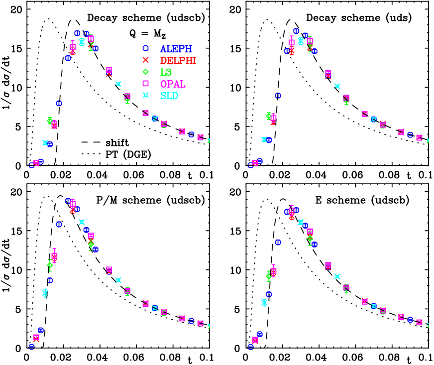
Figure 3: Thrust data at ${M_{\rm Z}}$ in the peak region together with shift-based fits using the range $0.05\,{M_{\rm Z}}/Q<t<0.30$ (dashed line) in different HMS. The perturbative calculation (DGE) is also shown (dotted line).

The results of fitting $\alpha_{s}$ and $\lambda_{1}$ to the data are summarized in Table 1. The global impact of ignoring the difference between heavy and light primary quarks on the fit is very small and it will be neglected in most of the following analysis. This does not imply, of course, that the effect is small at low energies. It is quite clear that it is significant at $14$ GeV, but the weight of these data in the fit is small. The table also shows that different HMS yield very similar values of $\alpha_{s}$ (the differences are less than $1.5\%$), whereas $\lambda_{1}$ changes by a factor of $\sim 2$.

Table 1: Fits of $\alpha_{s}$ and $\lambda_{1}$ to the thrust data with a lower cut $t_{\min}=0.05\,{M_{\rm Z}}/Q$ and an upper cut $t_{\max}=0.30$ in different HMS.

HMS	$\alpha_{\overline{\mbox{\tiny MS}}}({M_{\rm Z}})$	$\lambda_{1}\bar{\Lambda}$ [GeV]	$\chi^{2}/{\rm dof}$	Points
M/P (udscb)	0.1072 $\pm$ 0.0004	0.35 $\pm$ 0.02	0.58	159
M/P (uds)	0.1074 $\pm$ 0.0005	0.31 $\pm$ 0.02	0.58	159
E (udscb)	0.1080 $\pm$ 0.0004	0.42 $\pm$ 0.02	0.51	159
E (uds)	0.1082 $\pm$ 0.0004	0.38 $\pm$ 0.02	0.51	159
D (udscb)	0.1086 $\pm$ 0.0004	0.63 $\pm$ 0.02	0.43	159
D (uds)	0.1088 $\pm$ 0.0004	0.59 $\pm$ 0.02	0.45	159

The stability of $\alpha_{s}$ is very important: a physical parameter must not depend on arbitrary choices such as the particular definition of the variable or the “hadron level”. Note that stability was not reached in [24], when extracting $\alpha_{s}$ from mean values of event-shape variables. Analysing the distribution is advantageous, since the dependence on the variable, in addition to the energy, constrains $\alpha_{s}$ further. We have explicitly checked, performing a NLL fit (with $\log R$ matching) to the distribution that the results show the same stability as in the DGE case. From the table it is also clear that the decay scheme gives the best fits. We will mainly use this HMS in the following.

Next, we consider the dependence on the lower cut of the fit, $t_{\min}$. The results are summarized in Table 2. Note that for $t_{\min}\geq 0.05\,{M_{\rm Z}}/Q$ the results are stable: all fits for larger $t_{\min}$ agree within errors with the result for $t_{\min}=0.05\,{M_{\rm Z}}/Q$.

Table 2: Fits of $\alpha_{s}$ and $\lambda_{1}$ to the thrust data in the decay scheme (udscb) as a function of the lower cut $t_{\min}=t_{\min}({M_{\rm Z}})\,{M_{\rm Z}}/Q$ with the upper cut fixed as $t_{\max}=0.30$.

$t_{\min}({M_{\rm Z}})$	$\alpha_{\overline{\mbox{\tiny MS}}}({M_{\rm Z}})$	$\lambda_{1}\bar{\Lambda}$ [GeV]	$\chi^{2}/{\rm dof}$	Points
0.03	0.1075 $\pm$ 0.0002	0.69 $\pm$ 0.01	0.55	190
0.04	0.1075 $\pm$ 0.0003	0.69 $\pm$ 0.01	0.54	173
0.05	0.1086 $\pm$ 0.0004	0.63 $\pm$ 0.02	0.43	159
0.06	0.1091 $\pm$ 0.0005	0.60 $\pm$ 0.03	0.42	147
0.07	0.1091 $\pm$ 0.0007	0.60 $\pm$ 0.04	0.45	135
0.08	0.1090 $\pm$ 0.0007	0.61 $\pm$ 0.04	0.43	124
0.09	0.1086 $\pm$ 0.0009	0.64 $\pm$ 0.06	0.45	111
0.10	0.1084 $\pm$ 0.0011	0.65 $\pm$ 0.07	0.48	104

This means that there is essentially no dependence on the lower cut (it is less than $0.5\%$), provided that the cut is far enough above the peak region.

We have checked that varying the upper cut $t_{\max}$ between $0.15$ and $0.35$, while keeping the lower cut $t_{\min}=0.05\,M_{\rm Z}/Q$ fixed, the results for $\alpha_{\overline{\mbox{\tiny MS}}}({M_{\rm Z}})$ and $\lambda_{1}$ agree, within errors, with the results obtained for $t_{\max}=0.30$. Thus, the dependence on the upper cut is also negligible (less than $0.5\%$).

To demonstrate the importance of using data for all particles rather than for charged particles only, we made a separate fit to the ALEPH and DELPHI data at ${M_{\rm Z}}$ in the P scheme. The result changes from $\alpha_{\overline{\mbox{\tiny MS}}}({M_{\rm Z}})=0.1079\pm 0.0005$ and $\lambda_{1}\bar{\Lambda}=0.33\pm 0.03$ GeV with $\chi^{2}/{\rm dof}=0.45$ for all particles, to $\alpha_{\overline{\mbox{\tiny MS}}}({\rm M_{Z}})=0.1091\pm 0.0005$ and $\lambda_{1}\bar{\Lambda}=0.27\pm 0.03$ GeV with $\chi^{2}/{\rm dof}=0.62$ for charged particles. Thus, the difference in the fit results is small, but not negligible. However, there is a significant difference in the quality of the fit: in addition to the lower $\chi^{2}/{\rm dof}$, the sensitivity to varying the cuts on the fitting range is much lower. This concerns in particular the lower cut – compare Table 2 above with Table 2 in [9].

Finally, knowing that beyond the large-$\beta_{0}$ limit power corrections are modified by logarithmic $Q$ dependence [9], it is interesting to look for logarithmic $Q$ dependence of $\lambda_{1}$ by performing separate fits at each energy. Additional motivation for such investigation is provided by the finding of [24] that the scale dependence of hadron-mass related non-perturbative effects is enhanced by a factor of $\ln^{A}({Q}/{\bar{\Lambda}})$, where $A=1.565$. Fixing $\alpha_{s}$ to the value obtained by fitting all energies, we fitted $\lambda_{1}$ separately for each energy. The results of these fits in the decay and P schemes are shown in Fig. 4, along with a fitted line of the form $\lambda_{1}\bar{\Lambda}=p_{1}+p_{2}\ln({Q}/{\bar{\Lambda}})$. The best-fit values of $p_{1}$ and $p_{2}$ are

$${\rm D\;(udscb):} p_{1}=0.13\pm 0.11 p_{2}=0.08\pm 0.02$$

GeV

GeV,

(44)

$${\rm P\;(udscb):} p_{1}=-0.16\pm 0.12 p_{2}=0.08\pm 0.02$$

GeV

GeV.

(47)

The results show some trend of increase in $\lambda_{1}$, but the power of the logarithmic dependence cannot be extracted from the data. The difference between the decay and P schemes appears to be large, but independent of $Q$. In the following we will ignore the logarithmic $Q$ dependence and, instead, concentrate on fits with a shape function and the determination of $\lambda_{2}$.

Figure 4: The $Q$-dependence of the shift $\lambda_{1}$ for a fixed $\alpha_{s}$ in the decay and P schemes. The lines are fits of the form $\lambda_{1}\bar{\Lambda}=p_{1}+p_{2}\ln({Q}/{\bar{\Lambda}})$.

To summarize, the best fit values of $\alpha_{s}$ and $\lambda_{1}$ when using the decay scheme with all primary quarks, are

$${\rm D\;(udscb):} \alpha_{\overline{\mbox{\tiny MS}}}({M_{\rm Z}})=0.1086\pm 0.0004 \lambda_{1}\bar{\Lambda}=0.63\pm 0.02$$

GeV

(50)

with $\chi^{2}/{\rm dof}=0.43$. These values were found to be stable under variations of the lower and upper cuts of the fitting range and to have very small uncertainty due to heavy primary quarks. The uncertainty in the determination of $\alpha_{s}$ based on varying the HMS was found to be $\sim 2\%$. The shift $\lambda_{1}$ can be a meaningful parameter only when the HMS has been fixed, in which case it is determined up to $5$ – $10$% depending on the fitting range and the effect of heavy primary quarks. In the different schemes we considered, $\lambda_{1}$ changes by up to a factor $\sim 2$, giving an indication on the significance of hadron mass effects.

3.1.2 Fits with a shape function

Fitting with a shape function has the advantage that the peak region can be included in the analysis and the structure of subleading power corrections can be detected. While the motivation is to extend the fitting range as much as possible, the region $t\simeq\bar{\Lambda}/Q$, where all powers are equally important, must be avoided. Similarly to [9], these considerations lead us to choose $t_{\min}=0.01\,M_{\rm Z}/Q\simeq 4\bar{\Lambda}/Q$. The following fits are made to data in the decay scheme (with all primary quarks).

For the functional form of the shape function (39), we use two different possibilities for the fall-off at large $\zeta$: exponential and Gaussian. The results for an exponential fall-off are:

$${\rm D\;(udscb):} \alpha_{\overline{\mbox{\tiny MS}}}({M_{\rm Z}})=0.1090\pm 0.0004 \lambda_{1}\bar{\Lambda}=0.605\pm 0.013\;\;{\rm GeV} \lambda_{2}\bar{\Lambda}^{2}=0.002\pm 0.024\;\;{\rm GeV}^{2} b_{1}=0.61\pm 0.10 b_{2}\equiv 0\;\;{\rm(fixed)} q=1.55\pm 0.11$$

(55)

with $\chi^{2}/{\rm dof}=0.53$ for 225 points, and those for a Gaussian fall-off:

$${\rm D\;(udscb):} \alpha_{\overline{\mbox{\tiny MS}}}({M_{\rm Z}})=0.1085\pm 0.0004 \lambda_{1}\bar{\Lambda}=0.625\pm 0.011\;\;{\rm GeV} \lambda_{2}\bar{\Lambda}^{2}=-0.049\pm 0.018\;\;{\rm GeV}^{2} b_{1}\equiv 0\;\;{\rm(fixed)} b_{2}=0.028\pm 0.004 q=0.77\pm 0.08$$

(60)

with $\chi^{2}/{\rm dof}=0.58$ for 225 points. Both results are in good agreement with the shift-based fits for $t_{\min}\geq 0.05\,{M_{\rm Z}}/Q$ (50). As was the case in our earlier analysis, the best fit turns out to have an exponential fall-off. The Gaussian fall-off gives a slightly worse $\chi^{2}$. In addition, the softer, exponential fall-off is closer to the asymptotic behaviour found in [18] in a calculation of the shape function using a perturbative model.

The sensitivity to the functional form gives a good indication of the difficulty in determining $\lambda_{2}$ and higher moments of the shape function from the data in the absence of more definite theoretical input. The results of the exponential fall-off fit, which is the best fit, are in agreement with the large $\beta_{0}$ renormalon ambiguity pattern, which suggests that $\lambda_{2}=0$, but this is not true for the Gaussian fall-off. Nevertheless, in both cases $\lambda_{2}\ll\lambda_{1}^{2}$. Thus, if $\lambda_{1}\bar{\Lambda}$ is used as a reference scale for the non-perturbative parameters, then $\lambda_{2}$ is always small. One should also keep in mind that the value of $\lambda_{2}$ is strongly correlated to the values of $\alpha_{s}$ and $\lambda_{1}$. For example, fixing the values of $\alpha_{s}$ and $\lambda_{1}$ according to the fit with an exponential fall-off when fitting with a Gaussian fall-off the result is $\lambda_{2}\bar{\Lambda}^{2}=-0.020\pm 0.009$ GeV², which agrees, within errors, with the result for a exponential fall-off.

We have also verified that the result of the shape-function-based fit is not sensitive to the fitting range. This is true for $\alpha_{s}$ as well as for the non-perturbative parameters $\lambda_{1}$ and $\lambda_{2}$. In particular, the dependence on the lower cut $t_{\min}$ is summarized in Table 3. It is interesting to note that the fact that $\lambda_{2}$ is small can be deduced even if the region to the left of the distribution peak is excluded from the fit.

Table 3: Fits of $\alpha_{\overline{\mbox{\tiny MS}}}(M_{\rm Z})$ and shape function with exponential fall-off to the thrust data in the decay scheme (udscb) as a function of the lower cut $t_{\min}=t_{\min}(M_{\rm Z})M_{\rm Z}/Q$ with the upper cut $t_{\max}=0.30$ fixed.

$t_{\min}(M_{\rm Z})$	$\alpha_{\overline{\mbox{\tiny MS}}}({M_{\rm Z}})$	$\lambda_{1}\bar{\Lambda}$ [GeV]	$\lambda_{2}\bar{\Lambda}^{2}$ [GeV2]	$\chi^{2}/{\rm dof}$	Points
0.01	0.1090$\pm$ 0.0004	0.605 $\pm$ 0.013	0.002 $\pm$ 0.024	0.53	225
0.02	0.1088$\pm$ 0.0004	0.619 $\pm$ 0.015	-0.004 $\pm$ 0.023	0.48	209
0.03	0.1089$\pm$ 0.0004	0.618 $\pm$ 0.016	-0.001 $\pm$ 0.023	0.47	190
0.04	0.1089$\pm$ 0.0006	0.623 $\pm$ 0.040	0.015 $\pm$ 0.093	0.42	173

Figure 5 shows the data at ${M_{\rm Z}}$ in the decay scheme together with the best shape-function-based fit (55) and a shift-based fit. For the latter we use the range $0.06\,{M_{\rm Z}}/Q<t<0.30$, which gives the same $\alpha_{s}$ as the shape-function fit (see Table 2). The figure illustrates clearly the hierarchy between power corrections as a function of $t$. For large $t$ the shape function is well approximated by a shift. In the peak region the non-perturbative corrections with higher power become important, but the effects are still small. Finally, below the peak all power corrections become equally important.

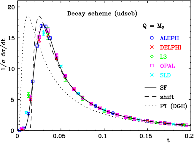
Figure 5: Thrust data at ${M_{\rm Z}}$ in the decay scheme together with the best shape-function-based fit (solid line) and a shift-based fit using the range $0.06\,{M_{\rm Z}}/Q<t<0.30$ (dashed line). The DGE perturbative calculation is also shown (dotted line).

For illustration, the best shape-function-based fit (55) is also shown at all energies, together with the data, in Fig. 6.

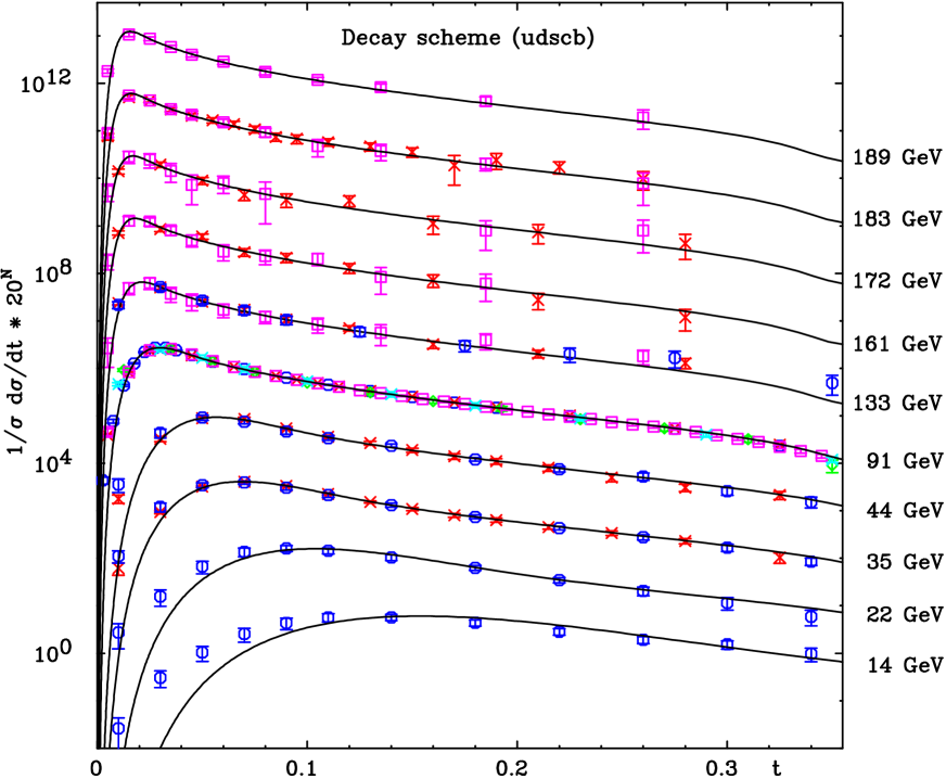
Figure 6: Comparison of the thrust data in the decay scheme with the best fit shape function. Both the fit and the data have been multiplied by a factor $20^{N}$, with $N=0\ldots 9$ for $Q=14\ldots 189$ GeV. Data points with errors larger than 100% are not shown.

The contribution to the $\chi^{2}$ from the individual experiments for the best shape-function-based fit (55) and the shift-based fit is given in Table 4. The fits are good at all energies, except at $14$ GeV. This exception is not surprising, since the effects of heavy quarks were not taken into account.

To investigate the effects of heavy primary quarks we have also performed the shape-function-based fit to the data which was transformed according to (41), so as to remove heavy-quark events from the data sample. As before, this transformation has been made using the Pythia Monte Carlo model. The results using a shape function with exponential fall-off, are

$${\rm D\;(uds):} \alpha_{\overline{\mbox{\tiny MS}}}({M_{\rm Z}})=0.1092\pm 0.0004 \lambda_{1}\bar{\Lambda}=0.568\pm 0.013\;\;{\rm GeV} \lambda_{2}\bar{\Lambda}^{2}=0.005\pm 0.023\;\;{\rm GeV}^{2} b_{1}=0.64\pm 0.10 b_{2}\equiv 0 q=1.51\pm 0.12$$

(65)

with $\chi^{2}/{\rm dof}=0.63$ for 225 points. This shows (cf. Table 1) that the effect of heavy quarks is slightly larger in the peak region with respect to higher $t$, but it is still small.

Considering the contribution to the $\chi^{2}$ from the individual experiments, that of $14$ GeV becomes only slightly smaller ($14.1\to 12.2$) whereas all the others increase. The Monte Carlo results suggest that the effect of heavy quarks is small, except at 14 GeV, in agreement with [31]. However, the change in $\chi^{2}$ raises doubts concerning the reliability of using the Monte Carlo together with Eq. (41) to quantify this effect. It is clear that there is place for improving the analysis in this respect.

Finally, we give the results of a fit with a shape function with exponential fall-off to the data in the P scheme:

$${\rm P\;(udscb):} \alpha_{\overline{\mbox{\tiny MS}}}({M_{\rm Z}})=0.1068\pm 0.0004 \lambda_{1}\bar{\Lambda}=0.388\pm 0.013\;\;{\rm GeV} \lambda_{2}\bar{\Lambda}^{2}=0.069\pm 0.022\;\;{\rm GeV}^{2} b_{1}=0.47\pm 0.05 b_{2}\equiv 0 q=0.73\pm 0.08$$

(70)

with $\chi^{2}/{\rm dof}=0.67$ for 225 points. This result agrees reasonably well with the shift-based fit in Table 1. The fact that here, in contrast to (55), the non-perturbative parameter $\lambda_{2}$ is significantly different from zero, $\lambda_{2}\sim\lambda_{1}^{2}$, is interesting. The differences between the non-perturbative parameters $\lambda_{n}$ in different HMS are associated with mass effects. It is rather clear that these effects, at least their non-universal parts [24], do not have a “perturbative” origin, and therefore it is not surprising that they do not admit the renormalon power correction pattern.

To summarize the fits with a shape function, the best fit in the decay scheme is (55), which agrees well with the shift-based fit (50). The second central moment $\lambda_{2}$ in this scheme is consistent with zero, in accordance with the large $\beta_{0}$ renormalon pattern. This is not the case in other HMS. Similarly to the shift-based fits, the only non-negligible source of uncertainty in $\alpha_{s}$ is the choice of HMS.

Table 4: Summary of the experimental data used and the contribution to $\chi^{2}$ from the individual experiments (in the decay scheme with all primary quarks). For the thrust, the data were fitted using a shift ($0.06\,{M_{\rm Z}}/Q<t<0.30$) and a shape function (SF) with exponential fall-off ($0.01\,{M_{\rm Z}}/Q<t<0.30$), whereas for the heavy-jet mass ($0.01\,{M_{\rm Z}}/Q<\rho_{H}<0.10$) the $\chi^{2}$ values were obtained with $\alpha_{\overline{\mbox{\tiny MS}}}({M_{\rm Z}})=0.109$ and with the shape function fixed according to the thrust analysis.

			thrust    shift		thrust      SF		heavy jet    SF
							($\alpha_{s}$ & SF fixed)
Experiment	Reference	Q [GeV]	$\chi^{2}$	Points	$\chi^{2}$	Points	$\chi^{2}$	Points
TASSO	[45, 46]	14	0.00	0	14.12	6	1.59	1
TASSO	[45, 46]	22	0.00	0	3.80	7	0.52	2
JADE	[47]	35	2.16	5	8.59	11	8.60	3
TASSO	[45, 46]	35	1.44	3	3.94	8	0.61	3
JADE	[47]	44	4.24	6	4.82	11	4.82	3
TASSO	[45, 46]	44	0.84	3	4.22	8	0.08	3
ALEPH	[48]	91.2	3.35	9	7.82	17	12.10	10
DELPHI	[49]	91.2	9.60	12	14.64	17	10.28	8
L3	[50]	91.2	3.67	7	3.90	9	6.15	5
OPAL	[51]	91.2	10.90	24	20.42	29	66.23	10
SLD	[52]	91.2	3.48	5	5.19	7	11.69	2
ALEPH	[53]	133	1.58	6	1.60	8
DELPHI	[54]	133	1.47	5	1.87	7	0.62	3
OPAL	[55]	133	2.16	6	2.51	10	2.09	6
DELPHI	[54]	161	3.47	6	4.81	7	1.06	3
OPAL	[56]	161	1.77	7	1.95	10	1.70	6
DELPHI	[54]	172	3.11	6	3.18	7	0.18	3
OPAL	[57]	172	2.14	7	2.31	10	2.74	7
DELPHI	[54]	183	4.22	14	4.84	16	0.62	7
OPAL	[57]	183	0.58	8	0.62	10	2.04	7
OPAL	[57]	189	0.94	8	1.40	10	2.32	7
Sum			61.1	147	116.5	225	136.0	99

3.1.3 Fits with a modified logarithm

To estimate the effects of the non-logarithmic terms, which are not included in the resummation, we repeat the calculation using a modified logarithm, $L=\ln(1/t-1)$ [2]. The results of fitting $\alpha_{s}$ and a shift $\lambda_{1}$ using the modified logarithm in different HMS is summarized in Table 5. Comparing with Table 1 we see that the central values of $\alpha_{s}$ are $\sim 2\%$ larger and $\lambda_{1}\bar{\Lambda}$ is $\sim 0.1$ GeV smaller, whereas the HMS dependence is unchanged. We also note that the $\chi^{2}$ values are significantly worse when using a modified logarithm.

Table 5: Fits of $\alpha_{s}$ and $\lambda_{1}$ to the thrust data with a lower cut $t_{\min}=0.05\,{M_{\rm Z}}/Q$ and an upper cut $t_{\max}=0.30$ in different hadron mass schemes using a modified logarithm, $L=\ln(1/t-1)$.

HMS	$\alpha_{\overline{\mbox{\tiny MS}}}({M_{\rm Z}})$	$\lambda_{1}\bar{\Lambda}$ [GeV]	$\chi^{2}/{\rm dof}$	Points
M/P (udscb)	0.1096 $\pm$ 0.0005	0.25 $\pm$ 0.03	0.70	159
E (udscb)	0.1104 $\pm$ 0.0005	0.32 $\pm$ 0.02	0.62	159
D (udscb)	0.1107 $\pm$ 0.0005	0.55 $\pm$ 0.02	0.50	159

In addition to the HMS dependence we have also investigated the dependence on the lower and upper cuts for the fit in the decay scheme. Recall that with the unmodified logarithm we found no dependence on these cuts outside the peak region. However, with the modified logarithm we find a large $t_{\min}$ dependence while keeping the upper cut fixed at $t_{\max}=0.30$. As shown in Table 6, changing the lower cut from $0.05\,{M_{\rm Z}}/Q$ to $0.10\,{M_{\rm Z}}/Q$, the result for $\alpha_{s}$ increases by $4\%$ and $\lambda_{1}\bar{\Lambda}$ decreases by $\sim 0.2$ GeV. The values only stabilize for $t_{\min}=0.07\,{M_{\rm Z}}/Q$, giving $\alpha_{\overline{\mbox{\tiny MS}}}({M_{\rm Z}})=0.113\pm 0.001$ and $\lambda_{1}\bar{\Lambda}=0.42\pm 0.04$. Likewise we find that keeping the lower cut fixed at $t_{\min}=0.07\,{M_{\rm Z}}/Q$ and varying the upper cut from $0.15$ to $0.35$ the result for $\alpha_{s}$ changes by $1.5\%$ and $\lambda_{1}\bar{\Lambda}$ by $\sim 0.05$ GeV.

Table 6: Modified logarithm ($L=\ln(1/t-1)$) fits of $\alpha_{s}$ and $\lambda_{1}$ to the thrust data in the decay scheme (udscb) as a function of the lower cut $t_{\min}=t_{\min}({M_{\rm Z}}){M_{\rm Z}}/Q$ with the upper cut fixed as $t_{\max}=0.30$.

$t_{\min}({M_{\rm Z}})$	$\alpha_{\overline{\mbox{\tiny MS}}}({M_{\rm Z}})$	$\lambda_{1}\bar{\Lambda}$ [GeV]	$\chi^{2}/{\rm dof}$	Points
0.03	0.1086 $\pm$ 0.0003	0.65 $\pm$ 0.01	0.73	190
0.04	0.1090 $\pm$ 0.0003	0.64 $\pm$ 0.01	0.72	173
0.05	0.1107 $\pm$ 0.0005	0.55 $\pm$ 0.02	0.50	159
0.06	0.1119 $\pm$ 0.0006	0.48 $\pm$ 0.03	0.44	147
0.07	0.1129 $\pm$ 0.0008	0.42 $\pm$ 0.04	0.45	135
0.08	0.1134 $\pm$ 0.0009	0.39 $\pm$ 0.05	0.44	124
0.09	0.1138 $\pm$ 0.0012	0.36 $\pm$ 0.08	0.46	111
0.10	0.1146 $\pm$ 0.0016	0.31 $\pm$ 0.10	0.48	104

Even though the fits with a modified logarithm are significantly worse than the fits with an unmodified logarithm these results can be used to estimate the significance of the non-logarithmic terms. Based on this we conclude that the effects of non-logarithmic terms can be as large as $4\%$ in $\alpha_{s}$ (from $\alpha_{\overline{\mbox{\tiny MS}}}({M_{\rm Z}})=0.109$ to $0.113$). This is by far the dominant contribution to theoretical uncertainty. We emphasize that this is a rough estimate and full NNLO calculations are essential to reduce the uncertainty.

3.2 Heavy jet mass distribution

As explained in section 2.3, the approximation we use for the phase space breaks down completely at $\rho_{H}=1/6$. Contrary to the case of the thrust, non-logarithmic corrections reflecting additional kinematic constraints may be important at rather small values of $\rho_{H}$. This will be reflected in the independent phenomenological analysis of the heavy-jet mass distribution in section 3.2.1. We prefer to rely on the thrust analysis as much as possible and compare between the non-perturbative corrections to the two observables only in the limited region where the calculation of the heavy-jet mass distribution can be trusted. This is the purpose of section 3.2.2.

3.2.1 Independent fits

The purpose of this section is to confront the DGE resummed cross section and the suggested parameterization of power corrections with the heavy-jet mass distribution data and find how severe the limitations described in section 2.3 are in practice.

We begin by fitting $\alpha_{s}$ and a shift of the perturbative distribution (38). This should be applicable far enough above the peak region. However, since the region where the calculation can be trusted is strongly restricted from above, we end up with a rather narrow range. The upper cut will be chosen as $\rho_{\max}=0.15$. We will show that the lower cut can be as small as $\rho_{\min}=0.03\,{M_{\rm Z}}/Q$.

The dependence on the HMS and the effect of heavy primary quarks are summarized in Table 7. First of all we note that the extracted values of $\alpha_{s}$ are much smaller than for the thrust case. The reason is that our approximation tends to overestimate the higher order perturbative coefficients at large $\rho_{H}$: an example is provided by the NLO coefficient shown in Fig. 1. This statement will be further supported by studying the dependence on the fitting range (Table 9). It should also be kept in mind that, since the distribution is normalized, overestimating the cross section at large $\rho_{H}$ is compensated by underestimating it at low $\rho_{H}$. For the NLO coefficient the turnover point is $\rho_{H}\sim 0.05$.

Table 7: Fits of $\alpha_{s}$ and $\lambda_{1}$ to the heavy-jet mass data with a lower cut of $\rho_{\min}=0.03\,{M_{\rm Z}}/Q$ and an upper cut of $\rho_{\max}=0.15$ in different HMS.

HMS	$\alpha_{\overline{\mbox{\tiny MS}}}({M_{\rm Z}})$	$\lambda_{1}\bar{\Lambda}$ [GeV]	$\chi^{2}/{\rm dof}$	Points
P (udscb)	0.1009 $\pm$ 0.0006	0.58 $\pm$ 0.03	0.42	87
P (uds)	0.1012 $\pm$ 0.0008	0.55 $\pm$ 0.04	0.41	87
E (udscb)	0.1014 $\pm$ 0.0007	0.69 $\pm$ 0.04	0.44	87
E (uds)	0.1018 $\pm$ 0.0007	0.65 $\pm$ 0.04	0.43	87
D (udscb)	0.1019 $\pm$ 0.0007	0.88 $\pm$ 0.03	0.50	87
D (uds)	0.1020 $\pm$ 0.0007	0.85 $\pm$ 0.03	0.50	87
M (udscb)	0.1026 $\pm$ 0.0006	1.03 $\pm$ 0.03	0.56	87

Since the values of $\alpha_{s}$ obtained here are so different from the thrust case, it is no surprise that the values of the shift $\lambda_{1}$ differ by much as well. In any case, a meaningful comparison of these parameters requires the same value of $\alpha_{s}$ to be used. We will come back to such a comparison below.

We note that, similarly to the thrust case, the HMS dependence and the effects of primary heavy quarks on the value of $\alpha_{s}$ is small. The largest difference is between the P and the massive schemes. The differences between the two can be clearly seen in Fig. 7, where the fit results at ${M_{\rm Z}}$ in the different HMS are shown together with the data. In the massive scheme the contribution from the hadron masses themselves shifts the distribution to the right. In general, as in the thrust case, the HMS transformations modify both the position and the height of the peak. Note, however, that the decay and massive schemes are quite similar for the heavy-jet mass. The reason is that the only difference between the two is the definition of the thrust axis.

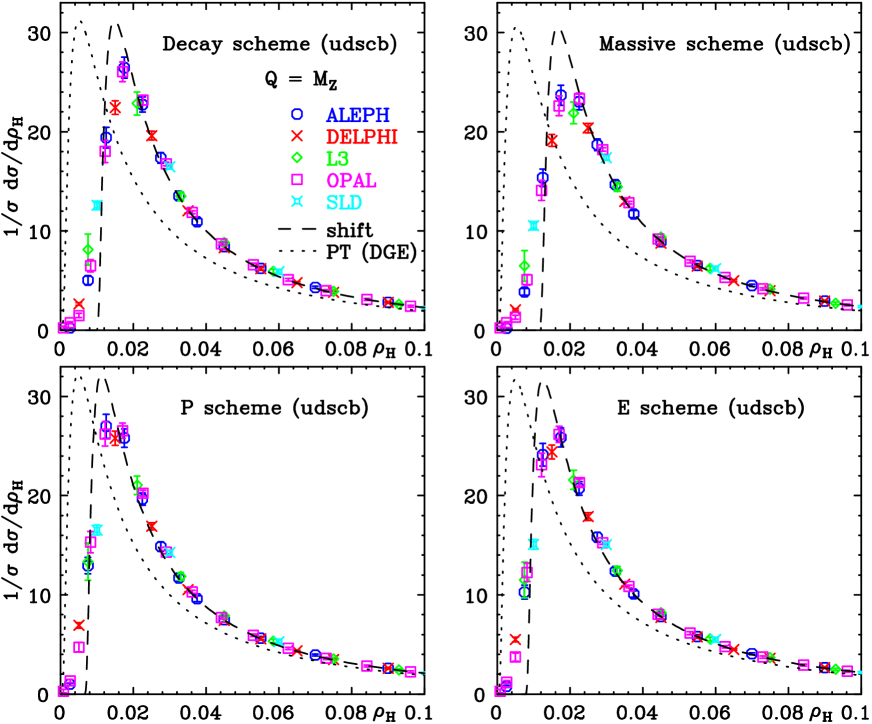
Figure 7: Heavy jet mass data at ${M_{\rm Z}}$ in the peak region together with shift-based fits using the range $0.03\,{M_{\rm Z}}/Q<\rho_{H}<0.15$ (dashed line) in different HMS. The perturbative calculation is also shown (dotted line).

Next, we investigate the variation of the result as a function of the fitting range in the decay scheme. From Tables 8 and 9, it can be concluded, based on the same criteria applied in the thrust analysis, that the maximal range that can be used is $0.03\,{M_{\rm Z}}/Q\leq\rho_{h}\leq 0.15$. However, contrary to the thrust case, here we identify a clear trend: as the fitting range shifts towards larger values of $\rho_{H}$, the value of $\alpha_{s}$ decreases. Thus, there is a systematic discrepancy between the shape of the theoretical distribution and the data. From Table 9 it is also clear that the fit deteriorates quickly for $\rho_{\max}>1/6$. This is a direct consequence of the missing kinematic constraints in the calculation (see Fig. 1).

Table 8: Fits of $\alpha_{s}$ and $\lambda_{1}$ to the heavy-jet mass data in the decay scheme (udscb) as a function of the lower cut $\rho_{\min}=\rho_{\min}({M_{\rm Z}}){M_{\rm Z}}/Q$, with the upper cut fixed as $\rho_{\max}=0.15$.

$\rho_{\min}({M_{\rm Z}})$	$\alpha_{\overline{\mbox{\tiny MS}}}({M_{\rm Z}})$	$\lambda_{1}\bar{\Lambda}$ [GeV]	$\chi^{2}/{\rm dof}$	Points
0.02	0.1009 $\pm$ 0.0005	0.94 $\pm$ 0.02	0.62	106
0.03	0.1019 $\pm$ 0.0007	0.88 $\pm$ 0.03	0.50	87
0.04	0.1023 $\pm$ 0.0010	0.86 $\pm$ 0.05	0.44	72
0.05	0.1012 $\pm$ 0.0014	0.95 $\pm$ 0.09	0.38	60
0.06	0.1000 $\pm$ 0.0019	1.05 $\pm$ 0.14	0.34	48
0.07	0.0990 $\pm$ 0.0031	1.12 $\pm$ 0.24	0.36	43

Table 9: Fits of $\alpha_{s}$ and $\lambda_{1}$ to the heavy-jet mass data in the decay scheme (udscb) as a function of the upper cut $\rho_{\max}$, with the lower cut fixed as $\rho_{\min}=0.03\,{M_{\rm Z}}/Q$.

$\rho_{\max}$	$\alpha_{\overline{\mbox{\tiny MS}}}({M_{\rm Z}})$	$\lambda_{1}\bar{\Lambda}$ [GeV]	$\chi^{2}/{\rm dof}$	Points
0.10	0.1028 $\pm$ 0.0009	0.86 $\pm$ 0.04	0.31	58
0.11	0.1027 $\pm$ 0.0009	0.87 $\pm$ 0.04	0.30	60
0.12	0.1024 $\pm$ 0.0008	0.87 $\pm$ 0.03	0.38	69
0.13	0.1023 $\pm$ 0.0008	0.87 $\pm$ 0.03	0.40	76
0.14	0.1021 $\pm$ 0.0007	0.88 $\pm$ 0.03	0.43	84
0.15	0.1019 $\pm$ 0.0007	0.88 $\pm$ 0.03	0.50	87
0.16	0.1014 $\pm$ 0.0006	0.90 $\pm$ 0.03	0.57	95
0.18	0.1006 $\pm$ 0.0006	0.92 $\pm$ 0.03	0.93	103
0.20	0.0995 $\pm$ 0.0005	0.95 $\pm$ 0.03	1.39	114

To demonstrate the importance of using data that have been corrected to be for all particles rather than for charged ones only, we made a separate fit to ALEPH and DELPHI data at ${M_{\rm Z}}$ in the massive scheme ($\rho_{\min}=0.03\,M_{\rm Z}/Q$ and $\rho_{\max}=0.15$). The result changes from $\alpha_{\overline{\mbox{\tiny MS}}}({M_{\rm Z}})=0.1039\pm 0.0009$ and $\lambda_{1}\bar{\Lambda}=0.95\pm 0.04$ GeV with $\chi^{2}/{\rm dof}=0.22$ for all particles, to $\alpha_{\overline{\mbox{\tiny MS}}}({M_{\rm Z}})=0.1086\pm 0.0007$ and $\lambda_{1}\bar{\Lambda}=0.88\pm 0.03$ GeV with $\chi^{2}/{\rm dof}=0.99$ for charged particles. Thus, contrary to the case of the thrust distribution, the difference in $\alpha_{s}$ is very significant. The agreement between the values of $\alpha_{s}$ between the thrust and heavy-jet mass distributions when fitting charged particles only should be regarded as accidental for the reason already given. Note that $\chi^{2}$ is much better for all particles than for charged particles only.

We have also performed fits to the experimental data using a shape function with exponential fall-off. For the lower cut $\rho_{\min}=0.01\,{M_{\rm Z}}/Q$ and the upper cut $\rho_{\max}=0.15$, we find

$${\rm D\;(udscb):} \alpha_{\overline{\mbox{\tiny MS}}}({M_{\rm Z}})=0.1020\pm 0.0005 \lambda_{1}\bar{\Lambda}=0.84\pm 0.03\;\;{\rm GeV} \lambda_{2}\bar{\Lambda}^{2}=-0.085\pm 0.032\;\;{\rm GeV}^{2} b_{1}=0.70\pm 0.10 b_{2}\equiv 0 q=0.50\pm 0.77$$

(75)

with $\chi^{2}/{\rm dof}=0.62$ for 132 points. For comparison we repeated the fit in the P scheme:

$${\rm P\;(udscb):} \alpha_{\overline{\mbox{\tiny MS}}}({M_{\rm Z}})=0.1008\pm 0.0006 \lambda_{1}\bar{\Lambda}=0.551\pm 0.012\;\;{\rm GeV} \lambda_{2}\bar{\Lambda}^{2}=-0.089\pm 0.015\;\;{\rm GeV}^{2} b_{1}=0.37\pm 0.02 b_{2}\equiv 0 q=10^{-7}\pm 0.11$$

(80)

with $\chi^{2}/{\rm dof}=0.47$ for 132 points. The results of these fits are in good agreement with the shift-based fits. This gives further support to the use of the lower cut $\rho_{\min}=0.03\,{M_{\rm Z}}/Q$ when fitting with a shift.

The results of the best fits with a shape function and with a shift (with lower cut $\rho_{\min}=0.03\,{M_{\rm Z}}/Q$) in the decay scheme are shown together with the data at ${M_{\rm Z}}$ in Fig. 8. The range shown is extended much above the upper cut in order to show the discrepancy discussed above between the calculation and the data.

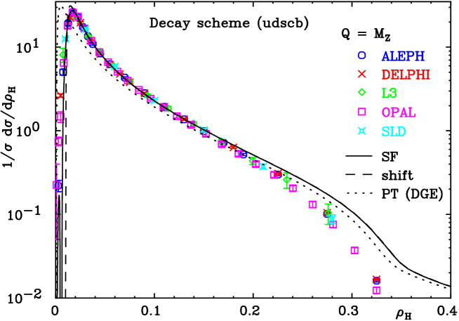
Figure 8: Heavy jet mass data at ${M_{\rm Z}}$ in the decay scheme for all primary quarks together with the results of the fits with a shape function in the range $0.01\,{M_{\rm Z}}/Q<\rho_{H}<0.15$ (solid line) and a shift in the range $0.03\,{M_{\rm Z}}/Q<\rho_{H}<0.15$ (dashed line). The perturbative calculation is also shown (dotted line).

Since the precision of the resummation formula deteriorates as $\rho_{H}$ is increased, we have also tried to decrease the upper cut $\rho_{\max}$ when fitting with a shape function. Limiting the fit to include just the peak region by choosing $\rho_{\max}=0.06$ (the fit does not converge for lower $\rho_{\max}$), the result is

$${\rm D\;(udscb):} \alpha_{\overline{\mbox{\tiny MS}}}({M_{\rm Z}})=0.1038\pm 0.0025 \lambda_{1}\bar{\Lambda}=0.78\pm 0.09\;\;{\rm GeV} \lambda_{2}\bar{\Lambda}^{2}=-0.057\pm 0.057\;\;{\rm GeV}^{2} b_{1}=0.45\pm 0.05 b_{2}\equiv 0 q=0.33\pm 0.45$$

(85)

with $\chi^{2}/{\rm dof}=0.55$ for 62 points. This shows that an analysis of the heavy-jet mass data restricted to the peak region is closer to the result from the thrust analysis. In addition, one identifies a trend for the central value of $\alpha_{s}$, which is similar to the shift-based fits: the lower the upper cut is, the higher $\alpha_{s}$ gets.

Finally, we have fitted $\alpha_{s}$ and a shift $\lambda_{1}$ to the heavy-jet mass data with a modified logarithm, $L=\ln(1/\rho_{H}-1)$. The effect of this modification is very small, because of the limited range used in the fit. As discussed in section (2.3), this modification does not at all represent the magnitude of genuine non-logarithmic terms in this case.

To summarize the independent fits to the heavy-jet mass distribution, we find smaller values of $\alpha_{s}$, and corresponding larger values of $\lambda_{1}$, than those obtained in the thrust analysis. We understand this discrepancy by the limited applicability of the phase-space approximation. We have established that this primarily affects the distribution at larger values of $\rho_{H}$. This is reflected for example in the fact that the best fit value of $\alpha_{s}$ decreases as the fitting range shifts to the right. Owing to the limitations of the currently available calculations, it is not possible to extract $\alpha_{s}$ reliably from the heavy-jet mass data. A full NNLO calculation can change the situation.

3.2.2 Comparison of the heavy-jet mass with thrust-based predictions

While the available calculation of the heavy-jet mass is not accurate far enough above the peak region to provide an independent measurement of $\alpha_{s}$, the main advantage of DGE is that it provides a solid basis for the analysis of power corrections in the peak region itself.

The purpose of this section is to test our assumptions concerning power corrections to the thrust and the heavy-jet mass distributions. This is done both by fitting the heavy-jet mass distribution with a fixed $\alpha_{s}$, which is set according to the best fit of the thrust, and comparing the power corrections parameters $\lambda_{n}$, as well as by using the best fits of the thrust distribution to determine all the parameters and confront the calculated heavy-jet mass distribution with the data.

We start by fitting a shift $\lambda_{1}$ of the perturbative heavy-jet mass distribution, for a fixed value of $\alpha_{s}$ based on the thrust fits (Table 1). The results are summarized in Table 10, together with the best fit values of $\lambda_{1}$ obtained in the thrust case for easy comparison. The agreement between the two observables is quite reasonable, except for the massive scheme, which is clearly disfavoured. We stress, however, that the heavy-jet mass results are quite sensitive to the fitting range and that the $\chi^{2}$ are much worse than in the fit where $\alpha_{s}$ is free. This is especially true for the data at ${M_{\rm Z}}$ where $\chi^{2}$/point $\mathrel{\raise 1.29167pt\hbox{$>$\kern-7.5pt\lower 4.30554pt\hbox{$\sim$}}}2$. The sensitivity to the upper and lower cuts is summarized in Tables 11 and 12, respectively. Examining Table 11 one can get the impression that the agreement of the shift parameters between the two observables shown in Table 10 is misleading, since the values strongly depend on the lower cut. Nevertheless, based on the shape-function fits presented below, the comparison in Table 11 is reliable: the shape-function-based fit values of $\lambda_{1}$ are consistent with those obtained with a shift, provided that the lower cut for the latter is $\rho_{\min}=0.03\,{M_{\rm Z}}/Q$.

Table 10: Fits of $\lambda_{1}$ to the heavy-jet mass data with a lower cut $\rho_{\min}=0.03\,{M_{\rm Z}}/Q$ and an upper cut $\rho_{\max}=0.15$ in different HMS using $\alpha_{\overline{\mbox{\tiny MS}}}({M_{\rm Z}})$ from the thrust analysis as input.

HMS	$\alpha_{\overline{\mbox{\tiny MS}}}({M_{\rm Z}})$	$\lambda_{1}\bar{\Lambda}$ [GeV]	$\chi^{2}/{\rm dof}$	Points	$(\lambda_{1}\bar{\Lambda})_{\rm thrust}$ [GeV]
P (udscb)	0.1072	0.28 $\pm$ 0.02	1.17	87	0.35 $\pm$ 0.02
E (udscb)	0.1080	0.38 $\pm$ 0.02	1.32	87	0.42 $\pm$ 0.02
D (udscb)	0.1086	0.59 $\pm$ 0.02	1.57	87	0.63 $\pm$ 0.02
M (udscb)	0.1072	0.85 $\pm$ 0.01	1.15	87	0.35 $\pm$ 0.02

Table 11: Fits of a shift with a fixed $\alpha_{\overline{\mbox{\tiny MS}}}({M_{\rm Z}})=0.1086$ to the heavy-jet mass data in the decay scheme (udscb) as a function of the lower cut $\rho_{\min}=\rho_{\min}({M_{\rm Z}})\,{M_{\rm Z}}/Q$, with a fixed upper cut $\rho_{\max}=0.15$.

$\rho_{\min}({M_{\rm Z}})$	$\lambda_{1}\bar{\Lambda}$ [GeV]	$\chi^{2}/{\rm dof}$	Points
0.02	0.70 $\pm$ 0.01	3.16	106
0.03	0.59 $\pm$ 0.02	1.57	87
0.04	0.51 $\pm$ 0.02	0.98	72
0.05	0.45 $\pm$ 0.03	0.79	60

Table 12: Fits of a shift with a fixed $\alpha_{\overline{\mbox{\tiny MS}}}({M_{\rm Z}})=0.1086$ to the heavy-jet mass data in the decay scheme (udscb) as a function of the upper cut $\rho_{\max}$ with a fixed lower cut $\rho_{\min}=0.03\,{M_{\rm Z}}/Q$.

$\rho_{\max}$	$\lambda_{1}\bar{\Lambda}$ [GeV]	$\chi^{2}/{\rm dof}$	Points
0.10	0.64 $\pm$ 0.02	0.95	58
0.11	0.63 $\pm$ 0.02	1.00	60
0.12	0.61 $\pm$ 0.02	1.27	69
0.13	0.61 $\pm$ 0.02	1.26	76
0.14	0.60 $\pm$ 0.02	1.47	84
0.15	0.59 $\pm$ 0.02	1.57	87
0.16	0.58 $\pm$ 0.02	1.94	95

To compare between the thrust and heavy-jet mass fits and to illustrate the correlation between $\alpha_{s}$ and $\lambda_{1}$, Fig. 9 shows the results of fitting the two parameters to the thrust and heavy-jet mass data in the decay scheme as 1-$\sigma$ contours. The figure also shows the results of fitting $\lambda_{1}$ for one of the observables when fixing $\alpha_{s}$ based on the other. We notice that the heavy-jet mass and thrust have very similar correlations between $\alpha_{s}$ and $\lambda_{1}$. In addition, the figure shows the results of the same exercise using NLL resummation, instead of DGE. Contrary to the DGE-based fits, in the NLL case there is no agreement between the thrust and heavy-jet mass results when $\alpha_{s}$ is fixed. This shows that important contributions are missed in the NLL resummation. In addition, the magnitude of the non-perturbative corrections for a given $\alpha_{s}$ is, of course, smaller in the case of DGE.

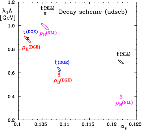
Figure 9: The results of fitting $\alpha_{s}$ and a shift $\lambda_{1}$ to the thrust and heavy-jet mass data in the decay scheme using DGE or NLL resummation (1-$\sigma$ contours). Also shown are the results of fitting $\lambda_{1}$ for one of the observables fixing $\alpha_{s}$ based on the other (crosses). The ranges used are $0.05\,{M_{\rm Z}}/Q<t<0.30$ and $0.03\,{M_{\rm Z}}/Q<\rho_{H}<0.15$.

A more stable result for the non-perturbative parameters under variations of the fitting range is obtained when including the peak region and fitting with a shape function. Fitting a shape function with an exponential fall-off in the decay scheme, where $\alpha_{s}$ is fixed based on the corresponding thrust analysis and the range is $0.01\,{M_{\rm Z}}/Q<\rho_{H}<0.10$, yields

$${\rm D\;(udscb):} \alpha_{\overline{\mbox{\tiny MS}}}({M_{\rm Z}})\equiv 0.1090\;\;{\rm fixed} \lambda_{1}\bar{\Lambda}=0.600\pm 0.007\;\;{\rm GeV} \lambda_{2}\bar{\Lambda}^{2}=0.080\pm 0.019\;\;{\rm GeV}^{2} b_{1}=0.50\pm 0.01 b_{2}\equiv 0 q=2\cdot 10^{-8}\pm 0.04$$

(90)

with $\chi^{2}/{\rm dof}=0.93$ for 99 points. The reduced sensitivity of the shape-function-based fit to the lower and upper cuts is shown in Tables 13 and 14, respectively. Note that fitting with a shape function only makes sense if the peak region is included. Therefore, the most relevant entries in Table 13 are the first two lines. The agreement with the thrust result (55) for $\lambda_{1}$ is very good. As for $\lambda_{2}$, although the $\rho_{H}$ fit results are not as stable with respect to the lower cut as those of the thrust (cf. Table 3), it seems that the $\rho_{H}$ fit in the decay scheme, as that of the thrust, prefers a small $\lambda_{2}$. For the parameter $b_{1}$ the agreement between the two results is also good, but this is not the case for $q$. It should also be noted that the value of $q$ in (90) is at the limit of the allowed range imposed on the fit.

Table 13: Fits of a shape function with a fixed $\alpha_{\overline{\mbox{\tiny MS}}}({M_{\rm Z}})=0.1090$ to the heavy-jet mass data in the decay scheme (udscb) as a function of the lower cut $\rho_{\min}=\rho_{\min}({M_{\rm Z}})\,{M_{\rm Z}}/Q$ with the upper cut $\rho_{\max}=0.10$ fixed.

$\rho_{\min}({M_{\rm Z}})$	$\lambda_{1}\bar{\Lambda}$ [GeV]	$\lambda_{2}\bar{\Lambda}^{2}$ [GeV2]	$\chi^{2}/{\rm dof}$	Points
0.01	0.60 $\pm$ 0.01	0.08 $\pm$ 0.02	0.93	99
0.02	0.60 $\pm$ 0.02	-0.01 $\pm$ 0.02	0.74	75
0.03	0.57 $\pm$ 0.01	-0.20 $\pm$ 0.07	0.37	58
0.04	0.39 $\pm$ 0.20	-0.29 $\pm$ 0.18	0.26	45

Table 14: Fits of a shape function with a fixed $\alpha_{\overline{\mbox{\tiny MS}}}({M_{\rm Z}})=0.1090$ to the heavy-jet mass data in the decay scheme (udscb) as a function of the upper cut $\rho_{\max}$ with the lower cut $\rho_{\min}=0.01\,{M_{\rm Z}}/Q$ fixed.

$\rho_{\max}$	$\lambda_{1}\bar{\Lambda}$ [GeV]	$\lambda_{2}\bar{\Lambda}^{2}$ [GeV2]	$\chi^{2}/{\rm dof}$	Points
0.05	0.63 $\pm$ 0.01	0.08 $\pm$ 0.02	0.58	52
0.10	0.60 $\pm$ 0.01	0.08 $\pm$ 0.02	0.93	99
0.15	0.58 $\pm$ 0.01	0.07 $\pm$ 0.02	1.45	132

Finally, as an ultimate test of our assumptions, we fix both $\alpha_{s}$ and the shape function based on the thrust distribution best fit and examine the agreement of the calculated heavy-jet mass distribution with the data. This gives a $\chi^{2}/{\rm dof}=1.37$ for $99$ points in the range $0.01\,{\rm M_{Z}}/Q<\rho_{H}<0.10$. The contribution to this $\chi^{2}$ from each experiment is shown in Table 4. It is worth noting that for most of the data sets the $\chi^{2}$ is good ($\chi^{2}\mathrel{\raise 1.29167pt\hbox{$<$\kern-7.5pt\lower 4.30554pt\hbox{$\sim$}}}1$). The only exceptions are JADE at $35$ GeV, OPAL at ${M_{\rm Z}}$ and SLD. Excluding these data sets the $\chi^{2}$ becomes $\chi^{2}/{\rm dof}=0.60$.

Figure 10 shows the data at ${M_{\rm Z}}$ together with the prediction based on the thrust analysis. The general agreement between the two is good. A closer look shows that the theory curve systematically underestimates the data up to $\rho_{H}\simeq 0.06$ and overestimates it to the right of this point.

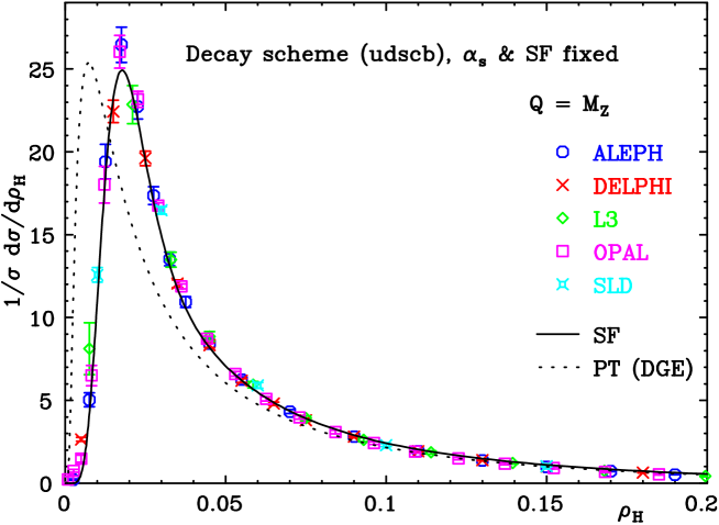
Figure 10: Comparison of the heavy-jet mass data at ${M_{\rm Z}}$ in the decay scheme with the theoretical prediction based on the determination of $\alpha_{s}$ and the shape function from the thrust analysis.

In Fig. 11 we show the prediction based on the thrust analysis together with the heavy-jet mass data at all energies. Here we see that the discrepancy between the predicted distribution and the $\rho_{H}$ data increases as the energy is decreased. This is natural, since the larger value of $\alpha_{s}$ makes the higher order corrections, which are unreliable for large $\rho_{H}$, more important.

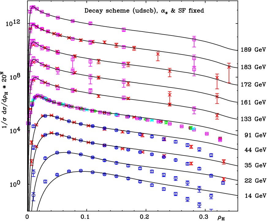
Figure 11: Comparison of the heavy-jet mass data in the decay scheme with the theoretical prediction based on the determination of $\alpha_{s}$ and the shape function from the thrust analysis. Both the theoretical prediction and the data have been multiplied by a factor $20^{N}$, with $N=0\ldots 9$ for $Q=14\ldots 189$ GeV. Data points with errors larger than $100~{}\%$ are not shown.

Finally, the non-perturbative parameters determined in a shape-function-based fit in the P scheme are also in very good agreement with the ones found in the thrust analysis, cf. Eq. (70), provided $\alpha_{s}$ is fixed by the latter:

$${\rm P\;(udscb):} \alpha_{\overline{\mbox{\tiny MS}}}({M_{\rm Z}})\equiv 0.1068\;\;{\rm fixed} \lambda_{1}\bar{\Lambda}=0.404\pm 0.007\;\;{\rm GeV} \lambda_{2}\bar{\Lambda}^{2}=0.080\pm 0.016\;\;{\rm GeV}^{2} b_{1}=0.37\pm 0.03 b_{2}\equiv 0 q=0.46\pm 0.07$$

(95)

with $\chi^{2}/{\rm dof}=0.82$ for 99 points. Although the total $\chi^{2}$ is good, the contribution from the experiments at ${M_{\rm Z}}$ is still larger than 2 per point. The result for $\lambda_{1}$ is rather stable with respect to variations of both the upper and lower cuts. The result for $\lambda_{2}$ turns out to be stable with respect to the upper cut, but, as in the decay scheme, not with respect to the lower cut. Fixing also the shape function to be the one found in the thrust analysis, the $\chi^{2}$ increases to $\chi^{2}/{\rm dof}=1.44$ for 99 points. In this case the $\chi^{2}$ is acceptable for all data sets except OPAL at ${M_{\rm Z}}$ and SLD, which contribute to $\chi^{2}$ $84$ for $10$ points and $13$ for $2$ points, respectively.

To summarize the comparison between the heavy-jet mass and the thrust, we find a good agreement between the two for the first moment of the shape function (or the shift) $\lambda_{1}$ once $\alpha_{s}$ is fixed. Although $\lambda_{2}$ is harder to determine, there is no indication for discrepancy between the observables even at this level. The agreement is restricted, of course, to the massless schemes (P, E and D). In general, the heavy-jet mass distribution in the peak region ($\rho_{H}\mathrel{\raise 1.29167pt\hbox{$<$\kern-7.5pt\lower 4.30554pt\hbox{$\sim$}}}0.1$) is well described by the theoretical prediction that uses $\alpha_{s}$ and the non-perturbative shape function from the thrust analysis as input. This supports our theoretical assumptions, in particular: using DGE as a basis for power correction analysis in the peak region (NLL resummation is insufficient), the assumption that the correlation between the hemisphere masses in the peak region is small (the simple relation between the thrust and the heavy-jet mass is based on no correlation) and, finally, the assumption that the non-perturbative corrections implied by the renormalon ambiguities dominate. In addition, we demonstrated how a careful treatment of hadron mass effects can open the way to quantitative comparison of hadronization effects which are parametrized as power corrections.

4 Conclusions

Dressed gluon exponentiation is especially designed to resum large perturbative corrections in differential cross sections in the threshold region, where power-suppressed corrections are non-negligible. DGE provides the basis for parametrization of these power corrections. Contrary to the standard Sudakov resummation techniques, which aim at a fixed logarithmic accuracy (such as NLL accuracy), DGE attempts to reach power accuracy. This does not mean, of course, that the perturbative calculation itself is correct to power accuracy (it is ambiguous at this level) but rather that the larger, perturbative corrections are resummed. These corrections appear as subleading Sudakov logs that are enhanced by numerical coefficients, which increase factorially at large orders.

Physically, the dominant perturbative corrections and the power corrections have the same source: soft gluon emission at large angles. Although both arise from integrals over the running coupling, one must separate between them, resum the former and parametrize the latter. A systematic separation is achieved, for example, by Borel summation. The sum of the two contributions is physically meaningful, but each of them separately is ambiguous. Moreover, subleading Sudakov logs (which are above the minimal term in the expansion) are parametrically larger than the ambiguous power correction, and their functional dependence on $Q$ and $\rho$ is distinct. Having realized this, it is clear that a meaningful comparison with data at power accuracy cannot be achieved with a fixed logarithmic accuracy. DGE is necessary.

Starting with the DGE calculation of the single-jet mass distribution in the approximation of independent emission, we expressed both the thrust and the heavy-jet mass distributions. Although the single-jet mass distribution is sensitive to non-inclusive contributions [39], both the thrust and the heavy-jet mass have a reduced sensitivity: Abelian non-inclusive contributions appear first at $\rm N^{(3)}LL$ order while non-Abelian ones do not appear before NNLL (see section 2.3).

An immediate consequence of the resummation of running-coupling effects by DGE is that the Sudakov exponent is renormalization-scale invariant within a given renormalization scheme. This is, of course, in contrast to NLL resummation. Fixing the renormalization scheme requires, in general, to fix $\Lambda$ as well as the renormalization-group equation for the coupling. Here $\Lambda$ was unambiguously fixed as $\bar{\Lambda}$ in the gluon bremsstrahlung scheme [33], accounting for the singular terms in the splitting function at next-to-leading order, which contribute to the thrust and the heavy-jet mass at the NLL level. On the other hand, the renormalization-group equation was arbitrarily chosen as the ‘t Hooft scheme, in which only the first two coefficients are non-vanishing. Consequently, renormalization-scheme dependence appears (through terms that are subleading in $\beta_{0}$) at NNLL order and beyond. Let us also recall that since renormalons are resummed only at the exponent, renormalization-scale dependence eventually appears when matching with the NLO result. Numerically these scheme and scale dependence effects are small and they are sub-dominant with respect to other theoretical uncertainties which are discussed below.

As discussed in [9], the DGE formula is suggestive of specific power corrections. First of all, the appearance of renormalon ambiguities in the exponent implies that power corrections also exponentiate, i.e. factorize in the Laplace space. This is compatible with the shape-function approach of [17]. To a first approximation, the non-perturbative correction amounts to a shift of the perturbative distribution [14, 23]. Secondly, assuming that renormalon-related power corrections dominate, intimate information on the shape function can be deduced from the singularity pattern of (2.2). The most striking property is the absence of a $\Lambda^{2}/(\rho Q)^{2}$ ambiguity in the exponent. This suggests that, if indeed power corrections follow the renormalon pattern, the second central moment of the shape function, $\lambda_{2}$, will be suppressed.

In addition to the non-perturbative corrections that can be inferred from the renormalon ambiguities, there are also finite hadron mass effects [24] that depend on the way masses are treated in the measurement of the variable. We saw that differences between different hadron mass schemes are of the same magnitude as the non-perturbative correction itself. Therefore, it is imperative that one uses the same HMS when comparing two variables and that this HMS is either insensitive to the masses or is defined such that the mass corrections for the two observables are similar. This qualifies the decay scheme as well as the E and the P scheme, but not the standardly used massive scheme. We found that, contrary to the case of average event shapes analysed in [24], the distributions analysed in different HMS yield very similar values for $\alpha_{s}$. The differences between different HMS can thus be naturally recast as a redefinition of the non-perturbative parameters.

Analysing the available thrust data, we obtained a best fit value of $\alpha_{\overline{\mbox{\tiny MS}}}({M_{\rm Z}})=0.109\pm 0.001$. This result is obtained both when fitting with a shift above the peak region and when fitting with a shape function. The consistency between the two procedures is reassuring. The main uncertainty in this result was found to be the effect of contributions suppressed by powers of $t$. It was estimated as $\sim 4$% by modifying the logarithm in the resummation from $\ln(1/t)$ to $\ln(1/t-1)$. The only other important uncertainty is due to the HMS dependence, which was found to be $\sim 2$%. There is, of course, some systematic uncertainty from the Monte Carlo model used to transform the data between different schemes, which we did not investigate. Other uncertainties, which we have investigated, turn out to be small: $\sim 0.5$%, i.e. comparable to the propagated experimental error. This includes: using a shift or a shape function, the form of the shape function, the fitting range, the residual renormalization scale dependence [9], and the effect of heavy quarks. The use of the Monte Carlo model in quantifying the latter is not satisfactory. All in all our estimate for the uncertainty in $\alpha_{s}$ is $\sim 5$%.

For the non-perturbative parameters of the shape function, our best fit values in the decay scheme (with all primary quarks) are $\lambda_{1}\bar{\Lambda}=0.605\pm 0.013$ GeV and $\lambda_{2}\bar{\Lambda}^{2}=0.002\pm 0.024$ GeV². The same value for $\lambda_{1}$ is obtained when fitting with shift. In other hadron mass schemes the value of $\lambda_{1}$ can be a factor $\sim 2$ lower. It is important to remember that the non-perturbative parameters are strongly correlated to $\alpha_{s}$. In a given HMS, with a fixed $\alpha_{s}$, the total uncertainty in $\lambda_{1}$ is less than $\sim 10$%. We also found a weak (logarithmic) energy dependence when fitting $\lambda_{1}$ separately at each energy. The second central moment of the shape function, $\lambda_{2}$, is correlated with both $\alpha_{s}$ and $\lambda_{1}$. Nevertheless, it is worth noting that in the best fit in the decay scheme $\lambda_{2}$ vanishes, in agreement with the large $\beta_{0}$ renormalon pattern. This finding can regarded as a success of the renormalon dominance assumption. However, one should be aware that it is not shared by other HMS: in the P scheme $\lambda_{2}$ is significantly different from zero. Hadron mass effects do not have a “perturbative” origin, and therefore they certainly do not admit the renormalon power correction pattern.

In the approximation of independent emission, soft gluons are radiated from a quark antiquark dipole. This naive phase space is useful to calculate the logarithmically enhanced terms, which are associated with this configuration. However, it misses kinematic constraints, which are present in the exact phase space. As discussed in section 2.3, this shows up as non-logarithmic corrections, which become important away from the two-jet limit. By examining our approximation versus the exact NLO calculation, we found that the thrust distribution is quite insensitive to such constraints, whereas the heavy-jet mass is. The difference between the heavy-jet mass and the thrust is well understood. The kinematic constraints imply correlations between the hemisphere masses: specifying the heavy-jet mass, as opposed to the thrust, puts a stringent constraint on the light jet mass. As a consequence, the logarithmic approximation to the heavy-jet mass distribution breaks down rather early, at $\rho_{H}=1/6$, and it is not as accurate as the equivalent calculation of the thrust distribution. Since the range of $\rho_{H}$ values where the resummation formula is valid is rather narrow, the determination of $\alpha_{s}$ from this distribution is unreliable: independent fits yield values of $\alpha_{s}$ significantly smaller than the thrust and values of $\lambda_{1}$ correspondingly larger. We showed that the distortion of the distribution mainly affects larger values of $\rho_{H}$. This is reflected for example in the fact that the best fit value of $\alpha_{s}$ decreases as the fitting range shifts to the right. Therefore, the comparison of non-perturbative corrections in the two-jet region between the heavy-jet mass and the thrust is still possible.

Since perturbatively the correlation between the hemispheres is significant only away from the two-jet limit, it is natural to assume that the correlation in the peak region is small also on the non-perturbative level. Under this assumption, a single non-perturbative shape function, which is associated with the single-jet mass, incorporates the dominant non-perturbative corrections to both the thrust and the heavy-jet mass distributions.

The deviation from this simple scenario was the subject of an interesting theoretical study and phenomenological analysis [17, 18]. It was claimed that correlation between the hemispheres due to non-perturbative soft-gluon emission is essential for a consistent description of the heavy-jet mass distribution in the peak region. Ref. [18] finds that, owing to radiation from one hemisphere into the other (“non-inclusive” correction) there is a positive correlation between the jet masses. It should be emphasized that this dynamical correlation, which is introduced in [17] through the shape function, has a similar flattening impact on the thrust distribution as on the $\rho_{H}$ distribution. Whereas radiation from one hemisphere into the other induces a positive correlation between the hemisphere masses, purely kinematic considerations indicate a negative correlation, which is missed by the logarithmic approximation for the heavy-jet mass distribution. As discussed in section 2.3, the latter seems to be the dominant feature limiting the accuracy of the calculation.

We assume here that the correlation between the hemispheres in the peak region is small and, we confront this assumption with the data. This is done is by using the best fits of the thrust distribution to determine $\alpha_{s}$ and the parameters of the shape function, and then confront the calculated heavy-jet mass distribution with the data. The consistency of the results shows that the correlation in the peak region is indeed small. An alternative approach we applied was to perform fits to the heavy-jet mass data, fixing $\alpha_{s}$ by the thrust analysis. We found a good agreement between the values of the shift $\lambda_{1}$ in the decay and E schemes, and a reasonable agreement in the P scheme (of course, the values differ by much in the massive scheme). Repeating the same exercise with the NLL resummation instead of DGE, we found a strong discrepancy between the thrust and heavy-jet mass results. The agreement of $\lambda_{1}$ between the thrust and the heavy-jet mass persists when fitting with a shape function. For the second central moment $\lambda_{2}$ the results are somewhat less conclusive, since it is sensitive to the fitting range and to the functional form of the shape function. Nevertheless, there is no indication for discrepancy between the observables even at this level.

It is of great interest to push the accuracy of the calculations further, e.g. by matching with a full NNLO result when it becomes avaliable. Some interesting questions could then be addressed in more detail. This includes, in particular, the consistency of the higher moments of the shape function with the renormalon pattern [9], the correlation between the hemispheres [17, 18], and hadron mass effects [24].

References

- [1] G. Sterman and S. Weinberg, Phys. Rev. Lett. 39 (1977) 1436.
- [2] S. Catani, G. Turnock, B. R. Webber and L. Trentadue, Phys. Lett. B263 (1991) 491.
- [3] S. Catani, L. Trentadue, G. Turnock and B. R. Webber, Nucl. Phys. B407 (1993) 3.
- [4] S. Catani, G. Turnock and B. R. Webber, Phys. Lett. B295 (1992) 269.
- [5] S. Catani and B. R. Webber, Phys. Lett. B427 (1998) 377 [hep-ph/9801350].
- [6] Y. L. Dokshitzer, A. Lucenti, G. Marchesini and G. P. Salam, JHEP 9801 (1998) 011 [hep-ph/9801324].
- [7] E. Gardi and G. Grunberg, JHEP 9911 (1999) 016 [hep-ph/9908458].
- [8] E. Gardi, JHEP 0004 (2000) 030 [hep-ph/0003179].
- [9] E. Gardi and J. Rathsman, Nucl. Phys. B609 (2001) 123 [hep-ph/0103217].
- [10] H. Contopanagos and G. Sterman, Nucl. Phys. B419 (1994) 77 [hep-ph/9310313].
- [11] A. V. Manohar and M. B. Wise, Phys. Lett. B344 (1995) 407 [hep-ph/9406392].
- [12] B. R. Webber, Phys. Lett. B339 (1994) 148 [hep-ph/9408222].
- [13] G. P. Korchemsky and G. Sterman, Nucl. Phys. B437 (1995) 415 [hep-ph/9411211].
- [14] G.P. Korchemsky and G. Sterman, Proc. 30th Rencontres de Moriond, QCD and high energy hadronic interactions, Les Arcs, Savoie, France, 1995, ed. J. Tran Thanh Van (Editions Frontières, Gif-sur-Yvette, 1995), p. 383 [hep-ph/9505391].
- [15] G. P. Korchemsky, Shape functions and power corrections to the event shapes, hep-ph/9806537.
- [16] G. P. Korchemsky and G. Sterman, Nucl. Phys. B555 (1999) 335 [hep-ph/9902341].
- [17] G. P. Korchemsky and S. Tafat, JHEP 0010 (2000) 010 [hep-ph/0007005].
- [18] A. V. Belitsky, G. P. Korchemsky and G. Sterman, Phys. Lett. B515 (2001) 297 [hep-ph/0106308].
- [19] Y. L. Dokshitzer and B. R. Webber, Phys. Lett. B352 (1995) 451 [hep-ph/9504219].
- [20] R. Akhoury and V. I. Zakharov, Phys. Lett. B357 (1995) 646 [hep-ph/9504248].
- [21] Y. L. Dokshitzer, A. Lucenti, G. Marchesini and G. P. Salam, JHEP 9805 (1998) 003 [hep-ph/9802381].
- [22] Y. L. Dokshitzer, G. Marchesini and B. R. Webber, Nucl. Phys. B469 (1996) 93 [hep-ph/9512336].
- [23] Y. L. Dokshitzer and B. R. Webber, Phys. Lett. B404 (1997) 321 [hep-ph/9704298].
- [24] G. P. Salam and D. Wicke, JHEP 0105 (2001) 061 [hep-ph/0102343].
- [25] E. Gardi, Nucl. Phys. B622 (2002) 365 [hep-ph/0108222].
-
[26]
S. J. Brodsky, G. P. Lepage and P. B. Mackenzie,
Phys. Rev. D28 (1983) 228.
G. P. Lepage and P. B. Mackenzie, Phys. Rev. D48 (1993) 2250 [hep-lat/9209022]. - [27] M. Beneke and V. M. Braun, Phys. Lett. B348 (1995) 513 [hep-ph/9411229].
- [28] P. Ball, M. Beneke and V. M. Braun, Nucl. Phys. B452 (1995) 563 [hep-ph/9502300].
- [29] S. J. Brodsky, E. Gardi, G. Grunberg and J. Rathsman, Phys. Rev. D63 (2001) 094017 [hep-ph/0002065].
- [30] H. Contopanagos, E. Laenen and G. Sterman, Nucl. Phys. B484 (1997) 303 [hep-ph/9604313].
- [31] P. A. Movilla Fernandez, S. Bethke, O. Biebel and S. Kluth, Eur. Phys. J. C 22 (2001) 1 [hep-ex/0105059].
- [32] D. E. Groom et al. [Particle Data Group Collaboration], Eur. Phys. J. C15 (2000) 1, and 2001 off-year partial update for the 2002 edition available on the PDG WWW pages (URL: http://pdg.lbl.gov/).
- [33] S. Catani, B. R. Webber and G. Marchesini, Nucl. Phys. B349 (1991) 635.
- [34] L. S. Brown and L. G. Yaffe, Phys. Rev. D45 (1992) 398.
- [35] L. S. Brown, L. G. Yaffe and C. Zhai, Phys. Rev. D46 (1992) 4712 [hep-ph/9205213].
- [36] M. Beneke, Nucl. Phys. B405 (1993) 424.
- [37] G. Grunberg, Phys. Lett. B304 (1993) 183.
- [38] P. Nason and M. H. Seymour, Nucl. Phys. B454 (1995) 291 [hep-ph/9506317].
- [39] M. Dasgupta and G. P. Salam, Phys. Lett. B512 (2001) 323 [hep-ph/0104277].
- [40] S. Catani and M.H. Seymour, Phys. Lett. B378 (1996) 287; Nucl. Phys. B485 (1997) 291; http://hepwww.rl.ac.uk/theory/seymour/nlo/
- [41] L. Clavelli and D. Wyler, Phys. Lett. B103 (1981) 383.
- [42] T. Sjöstrand, P. Eden, C. Friberg, L. Lönnblad, G. Miu, S. Mrenna and E. Norrbin, Comput. Phys. Commun. 135 (2001) 238 [hep-ph/0010017].
- [43] L. Lonnblad, Comput. Phys. Commun. 71 (1992) 15.
- [44] G. Corcella et al., JHEP 0101 (2001) 010 [hep-ph/0011363].
- [45] W. Braunschweig et al. [TASSO Collaboration], Z. Phys. C47 (1990) 187.
- [46] W. Braunschweig et al. [TASSO Collaboration], Z. Phys. C45 (1989) 11.
- [47] P. A. Movilla Fernandez, O. Biebel, S. Bethke, S. Kluth and P. Pfeifenschneider [JADE Collaboration], Eur. Phys. J. C1 (1998) 461 [hep-ex/9708034].
- [48] R. Barate et al. [ALEPH Collaboration], Phys. Rep. 294 (1998) 1.
- [49] P. Abreu et al. [DELPHI Collaboration], Eur. Phys. J. C14 (2000) 557 [hep-ex/0002026].
- [50] B. Adeva et al. [L3 Collaboration], Z. Phys. C55 (1992) 39.
- [51] P. D. Acton et al. [OPAL Collaboration], Z. Phys. C59 (1993) 1;
- [52] K. Abe et al. [SLD Collaboration], Phys. Rev. D51 (1995) 962 [hep-ex/9501003].
- [53] D. Buskulic et al. [ALEPH Collaboration], Z. Phys. C73 (1997) 409.
- [54] P. Abreu et al. [DELPHI Collaboration], Phys. Lett. B456 (1999) 322.
- [55] G. Alexander et al. [OPAL Collaboration], Z. Phys. C72 (1996) 191.
- [56] K. Ackerstaff et al. [OPAL Collaboration], Z. Phys. C75 (1997) 193.
- [57] G. Abbiendi et al. [OPAL Collaboration], Eur. Phys. J. C16, 185 (2000) [hep-ex/0002012].