Lepton Flavor Violating Processes

in Bi-maximal Texture of Neutrino Mixings

Atsushi Kageyama ,   Satoru Kaneko

Noriyuki Shimoyama ,   Morimitsu Tanimoto

Department of Physics, Niigata University, Ikarashi 2-8050, 950-2181 Niigata, JAPAN

ABSTRACT

We investigate the lepton flavor violation in the framework of the MSSM with right-handed neutrinos taking the large mixing angle MSW solution in the quasi-degenerate and the inverse-hierarchical neutrino masses. We predict the branching ratio of $\mu\rightarrow e+\gamma$ and $\tau\rightarrow\mu+\gamma$ processes assuming the degenerate right-handed Majorana neutrino masses. We find that the branching ratio in the quasi-degenerate neutrino mass spectrum is 100 times smaller than the ones in the inverse-hierarchical and the hierarchical neutrino spectra. We emphasize that the magnitude of $U_{e3}$ is one of important ingredients to predict BR($\mu\rightarrow e+\gamma$). The effect of the deviation from the complete-degenerate right-handed Majorana neutrino masses are also estimated. Furtheremore, we examine the $S_{3{\scriptscriptstyle L}}\times S_{3{\scriptscriptstyle R}}$ model, which gives the quasi-degenerate neutrino masses, and the Shafi-Tavartkiladze model, which gives the inverse-hierarchical neutrino masses. Both predicted branching ratios of $\mu\rightarrow e+\gamma$ are smaller than the experimantal bound.

1 Introduction

Super-Kamiokande has almost confirmed the neutrino oscillation in the atmospheric neutrinos, which favors the $\nu_{\mu}\rightarrow\nu_{\tau}$ process [1]. For the solar neutrinos [2, 3], the recent data of the Super-Kamiokande and the SNO also suggest the neutrino oscillation $\nu_{e}\rightarrow\nu_{\rm x}$ with the large mixing angle (LMA) MSW solution, although other solutions are still allowed [4, 5]. If we take the LMA-MSW solution, neutrinos are massive and the flavor mixings are almost bi-maximal in the lepton sector.

If neutrinos are massive and mixed in the SM, there exists a source of the lepton flavor violation (LFV) through the off-diagonal elements of the neutrino Yukawa coupling matrix. However, due to the smallness of the neutrino masses, the predicted branching ratios for these processes are so tiny that they are completely unobservable[6].

On the other hand, in the supersymmetric framework the situation is quite different. Many authors have already studied the LFV in the minimal supersymmetric standard model (MSSM) with right-handed neutrinos assuming the relevant neutrino mass matrix [7, 8, 9, 10]. In the MSSM with soft breaking terms, there exist lepton flavor violating terms such as off-diagonal elements of slepton mass matrices $\left({\bf m}^{2}_{\tilde{\scriptscriptstyle L}}\right)_{ij}$, $({\bf m}_{\tilde{e}_{\scriptscriptstyle R}}^{2})_{ij}$ and trilinear couplings ${\bf A}^{e}_{ij}$. Strong bounds on these matrix elements come from requiring branching ratios for LFV processes to be below observed ratios. For the present, the most stringent bound comes from the $\mu\rightarrow e+\gamma$ decay (${\rm BR}(\mu\rightarrow e+\gamma)<1.2\times 10^{-11}$) [11]. However, if the LFV occurs at tree level in the soft breaking terms, the branching ratio of this process exceeds the experimental bound considerably. Therefore one assumes that the LFV does not occur at tree level in the soft parameters. This is realized by taking the assumption that soft parameters such as $\left({\bf m}^{2}_{\tilde{\scriptscriptstyle L}}\right)_{ij}$, $({\bf m}_{\tilde{e}_{\scriptscriptstyle R}}^{2})_{ij}$, ${\bf A}^{e}_{ij}$, are universal i.e., proportional to the unit matrix. This assumption follows from the minimal supergravity (m-SUGRA). However, even though there is no flavor violation at tree level, it is generated by the effect of the renormalization group equations (RGE’s) via neutrino Yukawa couplings. Suppose that neutrino masses are produced by the see-saw mechanism [12], there are the right-handed neutrinos above a scale $M_{{\scriptscriptstyle R}}$. Then neutrinos have the Yukawa coupling matrix ${\bf Y}_{\nu}$ with off-diagonal entries in the basis of the diagonal charged-lepton Yukawa couplings. The off-diagonal elements of ${\bf Y}_{\nu}$ drive off-diagonal ones in the $\left({\bf m}_{\rm\tilde{\scriptscriptstyle L}}^{2}\right)_{ij}$ and ${\bf A}^{e}_{ij}$ matrices through the RGE’s running [13].

One can construct ${\bf Y}_{\nu}$ by the recent data of neutrino oscillations. Assuming that oscillations need only accounting for the solar and the atmospheric neutrino data, we take the LMA-MSW solution of the solar neutrino. Then, the lepton mixing matrix, which may be called the MNS matrix or the MNSP matrix [14, 15], is given in ref.[16]. Since the data of neutrino oscillations only indicate the differences of the mass square $\Delta m^{2}_{ij}$, neutrinos have three possible mass spectra: the hierarchical spectrum $m_{\nu 3}\gg m_{\nu 2}\gg m_{\nu 1}$ , the quasi-degenerate one $m_{\nu 1}\simeq m_{\nu 2}\simeq m_{\nu 3}$ and the inverse-hierarchical one $m_{\nu 1}\simeq m_{\nu 2}\gg m_{\nu 3}$.

We have already analyzed the effect of neutrino Yukawa couplings for the $\mu\rightarrow e+\gamma$ process assuming the quasi-degenerate one and the inverse-hierarchical one [17]. In this paper, we present detailed formula in our calculations of $\mu\rightarrow e+\gamma$ and discuss the dependence of the SUSY breaking parameters for the branching ratio. In the previous paper, the right-handed Majorana neutrino masses are assumed to be completely degenerate. We study the effect of the deviation from this degeneracy in this work. The correlation between BR($\mu\rightarrow e+\gamma$) and BR($\tau\rightarrow\mu+\gamma$) is also calculated. Furtheremore, two specific models of the neutrino mass matrix are examined in the $\mu\rightarrow e+\gamma$ process.

This paper is organized as follows. In section 2, we give the general form of ${\bf Y}_{\nu}$ and ${\bf Y}_{\nu}^{\dagger}{\bf Y}_{\nu}$, which play a crucial role in generating the LFV through the RGE’s running. In section 3, we calculate the branching ratio of the processes $\mu\rightarrow e+\gamma$ and $\tau\rightarrow\mu+\gamma$, respectively in the three neutrino mass spectra. In section 4, we examine the $S_{3{\scriptscriptstyle L}}\times S_{3{\scriptscriptstyle R}}$ model, which gives the quasi-degenerate neutrino masses, and the Shafi-Tavartkiladze model, which gives the inverse-hierarchical neutrino masses. In section 5, we summarize our results and give discussions.

2 LFV in the MSSM with Right-handed Neutrinos

2.1 Yukawa Couplings

In this section, we introduce the general expression of the neutrino Yukawa coupling ${\bf Y}_{\nu}$, which is useful in the following arguments, and investigate the LFV triggered by the neutrino Yukawa couplings. The superpotential of the lepton sector is described as follows:

$$W_{\rm lepton} = {\bf Y}_{e}LH_{d}e_{{\scriptscriptstyle R}}^{c}+{\bf Y_{\nu}}LH_{u}\nu_{{\scriptscriptstyle R}}^{c}+\frac{1}{2}{\nu_{\scriptscriptstyle R}^{c}}^{T}{\bf M_{\scriptscriptstyle R}}\nu_{\scriptscriptstyle R}^{c}\ ,$$ (2.1)

where $H_{u},H_{d}$ are chiral superfields for Higgs doublets, $L$ is the left-handed lepton doublet, $e_{\scriptscriptstyle R}$ and $\nu_{\scriptscriptstyle R}$ are the right-handed charged lepton and the neutrino superfields, respectively. The ${\bf Y}_{e}$ is the Yukawa coupling matrix for the charged lepton, ${\bf M_{\scriptscriptstyle R}}$ is Majorana mass matrix of the right-handed neutrinos. We take ${\bf Y}_{e}$ and ${\bf M_{\scriptscriptstyle R}}$ to be diagonal.

It is well-known that the neutrino mass matrix is given as

$${\bf m_{\nu}}=\left({\bf Y_{\nu}}v_{u}\right)^{\rm T}{\bf M}_{\bf{\scriptscriptstyle R}}^{-1}\left({\bf Y_{\nu}}v_{u}\right)\ ,$$ (2.2)

via the see-saw mechanism, where $v_{u}$ is the vacuum expectation value (VEV) of Higgs $H_{u}$. In eq.(2.2), the Majorana mass term for left-handed neutrinos is not included since we consider the minimal extension of the MSSM.

The neutrino mass matrix ${\bf m_{\nu}}$ is diagonalized by a single unitary matrix

$${\bf m_{\nu}^{{\scriptscriptstyle\rm diag}}} \equiv {\bf U}_{{\rm{\scriptscriptstyle M}{\scriptscriptstyle N}{\scriptscriptstyle S}}}^{\rm T}{\bf m_{\nu}}{\bf U_{{\rm{\scriptscriptstyle M}{\scriptscriptstyle N}{\scriptscriptstyle S}}}}\ ,$$ (2.3)

where ${\bf U_{{\rm{\scriptscriptstyle M}{\scriptscriptstyle N}{\scriptscriptstyle S}}}}$ is the lepton mixing matrix. Following the expression in ref.[10], we write the neutrino Yukawa coupling as

$${\bf Y_{\nu}}=\frac{1}{v_{u}}\sqrt{{\bf M_{\scriptscriptstyle R}^{{\scriptscriptstyle\rm diag}}}}\ {\bf R}\ \sqrt{{\bf m_{\nu}^{{\scriptscriptstyle\rm diag}}}}\ {\bf U}^{\rm T}_{{\rm{\scriptscriptstyle M}{\scriptscriptstyle N}{\scriptscriptstyle S}}}\ ,$$ (2.4)

or explicitly

$${\bf Y_{\nu}}=\frac{1}{v_{u}}\left(\matrix{\sqrt{M_{{\scriptscriptstyle R}1}}&0&0\cr 0&\sqrt{M_{{\scriptscriptstyle R}2}}&0\cr 0&0&\sqrt{M_{{\scriptscriptstyle R}3}}\cr}\right){\bf R}\left(\matrix{\sqrt{m_{\nu 1}}&0&0\cr 0&\sqrt{m_{\nu 2}}&0\cr 0&0&\sqrt{m_{\nu 3}}\cr}\right){\bf U}^{\rm T}_{{\rm{\scriptscriptstyle M}{\scriptscriptstyle N}{\scriptscriptstyle S}}}\ ,$$ (2.5)

where $\bf R$ is a $3\times 3$ orthogonal matrix, which depends on models. Details are given in Appendix A.

At first, let us take the degenerate right-handed Majorana masses $M_{{\scriptscriptstyle R}1}=M_{{\scriptscriptstyle R}2}=M_{{\scriptscriptstyle R}3}\equiv M_{R}$. This assumption is reasonable for the case of the quasi-degenerate neutrino masses. Otherwise a big conspiracy would be needed between ${\bf Y_{\nu}}$ and ${\bf M}_{\bf{\scriptscriptstyle R}}$. This assumption is also taken for cases of the inverse-hierarchical and the hierarchical neutrino masses. We also discuss later the effect of the deviation from the degenerate right-handed Majonara neutrino masses.

Then, we get

$${\bf Y_{\nu}}=\frac{\sqrt{M_{{\scriptscriptstyle R}}}}{v_{u}}\ {\bf R}\ \left(\matrix{\sqrt{m_{\nu 1}}&0&0\cr 0&\sqrt{m_{\nu 2}}&0\cr 0&0&\sqrt{m_{\nu 3}}\cr}\right){\bf U}^{\rm T}_{{\rm{\scriptscriptstyle M}{\scriptscriptstyle N}{\scriptscriptstyle S}}}\ ,$$ (2.6)

and

$${\bf Y_{\nu}^{\dagger}Y_{\nu}} = \frac{M_{\scriptscriptstyle R}}{v_{u}^{2}}{\bf U_{{\rm{\scriptscriptstyle M}{\scriptscriptstyle N}{\scriptscriptstyle S}}}}\left(\matrix{m_{\nu 1}&0&0\cr 0&m_{\nu 2}&0\cr 0&0&m_{\nu 3}\cr}\right){\bf U}_{{\rm{\scriptscriptstyle M}{\scriptscriptstyle N}{\scriptscriptstyle S}}}^{\rm T}\ ,$$ (2.7)

or equivalently,

$$\left({\bf Y_{\nu}^{\dagger}Y_{\nu}}\right)_{\alpha\beta} = \frac{M_{\scriptscriptstyle R}}{v_{u}^{2}}\sum_{i=1}^{3}m_{\nu i}U_{\alpha i}U_{\beta i}^{*}\ ,$$ (2.8)

where $U_{\alpha\beta}$’s are the elements of ${\bf U_{{\rm{\scriptscriptstyle M}{\scriptscriptstyle N}{\scriptscriptstyle S}}}}$. It is remarked that $\bf Y_{\nu}^{\dagger}Y_{\nu}$ is independent of $\bf R$ in the case of $M_{{\scriptscriptstyle R}1}=M_{{\scriptscriptstyle R}2}=M_{{\scriptscriptstyle R}3}\equiv M_{\scriptscriptstyle R}$. It may be important to consider the deviation from the degenerate right-handed Majonara neutrino masses. Detailed discussions are given in subsection 3.2.

Note that this representation of the Yukawa coupling is given at the electroweak scale. Since we need the Yukawa coupling at the GUT scale, eq.(2.5) should be modified by taking account of the effect of the RGE’s [18, 19, 20]. Modified Yukawa couplings at a scale $M_{\scriptscriptstyle R}$ are given as

$${\bf Y_{\nu}}=\frac{\sqrt{M_{\scriptscriptstyle R}}}{v_{u}}\ {\bf R}\ \left(\matrix{\sqrt{m_{\nu 1}}&0&0\cr 0&\sqrt{m_{\nu 2}}&0\cr 0&0&\sqrt{m_{\nu 3}}\cr}\right){\bf U}^{\rm T}_{{\rm{\scriptscriptstyle M}{\scriptscriptstyle N}{\scriptscriptstyle S}}}\sqrt{I_{g}I_{t}}\left(\matrix{1&0&0\cr 0&1&0\cr 0&0&\sqrt{I_{\tau}}\cr}\right)\ ,$$ (2.9)

with

$$I_{g}=\exp\left[\frac{1}{8\pi^{2}}\int_{t_{\scriptscriptstyle Z}}^{t_{\scriptscriptstyle R}}-c_{i}g_{i}^{2}dt\right]\ ,\quad I_{t}=\exp\left[\frac{1}{8\pi^{2}}\int_{t_{\scriptscriptstyle Z}}^{t_{\scriptscriptstyle R}}y_{t}^{2}dt\right]\ ,\quad I_{\tau}=\exp\left[\frac{1}{8\pi^{2}}\int_{t_{\scriptscriptstyle Z}}^{t_{\scriptscriptstyle R}}y_{\tau}^{2}dt\right]\ ,$$ (2.10)

where $t_{\scriptscriptstyle R}=\ln M_{\scriptscriptstyle R}$ and $t_{\scriptscriptstyle Z}=\ln M_{\scriptscriptstyle Z}$. Here, $g_{i}$’s$(i=1,2)$ are gauge couplings and $y_{t}$ and $y_{\tau}$ are Yukawa couplings, $c_{i}$’s are the constants $(\frac{3}{5},3)$. We shall calculate the LFV numerically by using the modified Yukawa coupling in the following sections.

As mentioned in the previous section, there are three possible neutrino mass spectra. The hierarchical type ($m_{\nu 1}\ll m_{\nu 2}\ll m_{\nu 3}$) gives the neutrino mass spectrum as

$$m_{\nu 1}\sim 0\ ,\qquad m_{\nu 2}=\sqrt{\Delta m^{2}_{\odot}}\ ,\qquad m_{\nu 3}=\sqrt{\Delta m^{2}_{\rm atm}}\ ,$$ (2.11)

the quasi-degenerate type ($m_{\nu 1}\sim m_{\nu 2}\sim m_{\nu 3}$) gives

$$m_{\nu 1}\equiv m_{\nu}\ ,\qquad m_{\nu 2}=m_{\nu}+\frac{1}{2m_{\nu}}\Delta m^{2}_{\odot}\ ,\qquad m_{\nu 3}=m_{\nu}+\frac{1}{2m_{\nu}}\Delta m_{\rm atm}^{2}\ ,$$ (2.12)

and the inverse-hierarchical type ($m_{\nu 1}\sim m_{\nu 2}\gg m_{\nu 3}$) gives

$$\quad m_{\nu 2}\equiv\sqrt{\Delta m^{2}_{\rm atm}}\ ,\quad m_{\nu 1}=m_{\nu 2}-\frac{1}{2m_{\nu 2}}\Delta m_{\odot}^{2}\ ,\quad m_{\nu 3}\simeq 0\ .$$ (2.13)

We take the typical values $\Delta m^{2}_{\rm atm}=3\times 10^{-3}{\rm eV}^{2}$ and $\Delta m_{\odot}^{2}=7\times 10^{-5}{\rm eV}^{2}$ in our calculation of the LFV.

We take the typical mixing angles of the LMA-MSW solution such as $s_{23}=1/\sqrt{2}$ and $s_{12}=0.6$ [16], in which the lepton mixing matrix is given in terms of the standard parametrization of the mixing matrix [23] as follows:

$${\bf U_{{\rm{\scriptscriptstyle M}{\scriptscriptstyle N}{\scriptscriptstyle S}}}}=\left(\matrix{c_{13}c_{12}&c_{13}s_{12}&s_{13}e^{-i\phi}\cr-c_{23}s_{12}-s_{23}s_{13}c_{12}e^{i\phi}&c_{23}c_{12}-s_{23}s_{13}s_{12}e^{i\phi}&s_{23}c_{13}\cr s_{23}s_{12}-c_{23}s_{13}c_{12}e^{i\phi}&-s_{23}c_{12}-c_{23}s_{13}s_{12}e^{i\phi}&c_{23}c_{13}\cr}\right)\ ,$$ (2.14)

where $s_{ij}\equiv\sin{\theta_{ij}}$ and $c_{ij}\equiv\cos{\theta_{ij}}$ are mixings in vacuum, and $\phi$ is the $CP$ violating phase. The reacter experiment of CHOOZ [21] presented a upper bound of $s_{13}$. We use the constraint from the two flavor analysis, which is $s_{13}\leq 0.2$ in our calculation. If we take account of the recent result of the three flavor analysis [22], the upper bound of $s_{13}$ may be smaller than 0.2. Then, if we use the results in [22], our results of $\mu\rightarrow e+\gamma$ are reduced at most by a factor of two. In our calculation, the CP violating phase is neglected for simplicity.

2.2 LFV in Slepton Masses

Since SUSY is spontaneously broken at the low energy, we consider the MSSM with the soft SUSY breaking terms:

$$-{\cal{L}}_{\rm soft} = ({\bf m}_{\tilde{\scriptscriptstyle Q}}^{2})_{ij}{\tilde{Q}}_{i}^{\dagger}{\tilde{Q}}_{j}+({\bf m}_{\tilde{u}}^{2})_{ij}{\tilde{u}}_{{\scriptscriptstyle R}i}^{*}{\tilde{u}}_{{\scriptscriptstyle R}j}+({\bf m}_{\tilde{d}}^{2})_{ij}{\tilde{d}}_{{\scriptscriptstyle R}i}^{*}{\tilde{d}}_{{\scriptscriptstyle R}j}$$ (2.15)

$$+({\bf m}_{\tilde{\scriptscriptstyle L}}^{2})_{ij}{\tilde{L}}_{i}^{\dagger}{\tilde{L}}_{j}+({\bf m}_{\tilde{e}}^{2})_{ij}{\tilde{e}}_{{\scriptscriptstyle R}i}^{*}{\tilde{e}}_{{\scriptscriptstyle R}j}+({\bf m}_{\tilde{\nu}}^{2})_{ij}{\tilde{\nu}}_{{\scriptscriptstyle R}i}^{*}{\tilde{\nu}}_{{\scriptscriptstyle R}j}$$

$$+{\widetilde{m}}^{2}_{H_{d}}H_{d}^{\dagger}H_{d}+{\widetilde{m}}^{2}_{H_{u}}H_{u}^{\dagger}H_{u}+(B\mu H_{d}H_{u}+\frac{1}{2}B_{\nu ij}M_{{\scriptscriptstyle R}ij}{\tilde{\nu}}_{{\scriptscriptstyle R}i}^{*}{\tilde{\nu}}_{{\scriptscriptstyle R}j}^{*}+h.c.)$$

$$+({\bf A}^{d}_{ij}H_{d}{\tilde{d}}_{{\scriptscriptstyle R}i}^{*}{\tilde{Q}}_{j}+{\bf A}^{u}_{ij}H_{u}{\tilde{u}}_{{\scriptscriptstyle R}i}^{*}{\tilde{Q}}_{j}+{\bf A}^{e}_{ij}H_{d}{\tilde{e}}_{{\scriptscriptstyle R}i}^{*}{\tilde{L}}_{j}+{\bf A}^{\nu}_{ij}H_{u}{\tilde{\nu}}_{{\scriptscriptstyle R}i}^{*}{\tilde{L}}_{j}$$

$$+\frac{1}{2}M_{1}{\tilde{B}}_{L}^{0}{\tilde{B}}_{L}^{0}+\frac{1}{2}M_{2}{\tilde{W}}_{L}^{a}{\tilde{W}}_{L}^{a}+\frac{1}{2}M_{3}{\tilde{G}}^{a}{\tilde{G}}^{a}+h.c.)\ ,$$

where ${\bf m}_{\tilde{Q}}^{2},{\bf m}_{\tilde{u}}^{2},{\bf m}_{\tilde{d}}^{2},{\bf m}_{\tilde{\scriptscriptstyle L}}^{2},{\bf m}_{\tilde{e}}^{2}$ and ${\bf m}_{\tilde{\nu}}^{2}$ are mass-squares of the left-handed squark, the right-handed up squark, the right-handed down squark, the left-handed charged slepton, the right-handed charged slepton and the sneutrino, respectively. The ${\widetilde{m}}^{2}_{H_{d}}$ and ${\widetilde{m}}^{2}_{H_{u}}$ are mass-squares of Higgs, ${\bf A}_{d},{\bf A}_{u},{\bf A}_{e}$ and ${\bf A}_{\nu}$ are A-parameters for squarks and sleptons, and $M_{1},M_{2}$ and $M_{3}$ are the gaugino masses, respectively.

Note that the lepton flavor violating processes come from diagrams including non-zero off-diagonal elements of the soft parameter. In this paper we assume the m-SUGRA, therefore we put the assumption of universality for soft SUSY breaking terms at the unification scale:

$$({\bf m}_{\tilde{\scriptscriptstyle L}}^{2})_{ij} = ({\bf m}_{\tilde{e}}^{2})_{ij}=({\bf m}_{\tilde{\nu}}^{2})_{ij}=\cdots=\delta_{ij}m_{0}^{2}\ ,$$

$${\widetilde{m}_{H_{d}}}^{2} = {\widetilde{m}_{H_{u}}}^{2}=m_{0}^{2}\ ,$$

$${\bf A}^{\nu} = {\bf Y}_{\nu}a_{0}m_{0},~{}{\bf A}^{e}={\bf Y}_{e}a_{0}m_{0}\ ,$$

$${\bf A}^{u} = {\bf Y}_{u}a_{0}m_{0},~{}{\bf A}^{d}={\bf Y}_{d}a_{0}m_{0}\ ,$$ (2.16)

where $m_{0}$ and $a_{0}$ stand for the universal scalar mass and the universal A-parameter, respectively. Because of the universality, the LFV is not caused at the unification scale.

To estimate the soft parameters at the low energy, we need to know the effect of radiative corrections. As a result, the lepton flavor conservation is violated at the low energy.

The RGE’s for the left-handed slepton soft mass are given by

$$\mu\frac{d}{d\mu}({\bf m}_{\tilde{\scriptscriptstyle L}}^{2})_{ij}=\left.\mu\frac{d}{d\mu}({\bf m}_{\tilde{\scriptscriptstyle L}}^{2})_{ij}\right|_{\rm MSSM}$$

$$+\frac{1}{16\pi^{2}}\left[({\bf m}_{\tilde{\scriptscriptstyle L}}^{2}{\bf Y}_{\nu}^{\dagger}{\bf Y}_{\nu}+{\bf Y}_{\nu}^{\dagger}{\bf Y}_{\nu}{\bf m}_{\tilde{\scriptscriptstyle L}}^{2})_{ij}+2({\bf Y}_{\nu}^{\dagger}{\bf m}_{\tilde{\nu}}{\bf Y}_{\nu}+{\tilde{m}}_{H_{u}}^{2}{\bf Y}_{\nu}^{\dagger}{\bf Y}_{\nu}+{\bf A}_{\nu}^{\dagger}{\bf A}_{\nu})_{ij}\right]\ ,$$

while the first term in the right hand side is the normal MSSM term which has no LFV, and the second one is a source of the LFV through the off-diagonal elements of neutrino Yukawa couplings. The RGE’s are summarized in Appendix B.

3 Numerical Analyses of Branching Ratios

Let us calculate the branching ratio of $e_{i}\rightarrow e_{j}+\gamma\ (j<i)$. The amplitude of this process is given as

$$T=e\epsilon^{\alpha*}(q)\overline{u}_{j}(p)m_{e_{i}}i\sigma_{\alpha\beta}q^{\beta}(A^{{\scriptscriptstyle L}}P_{{\scriptscriptstyle L}}+A^{{\scriptscriptstyle R}}P_{{\scriptscriptstyle R}})u_{i}(q-p)\ ,$$ (3.1)

where $u_{i}$ is the wave function of $i$-th charged lepton $e_{i}$, $p$ and $q$ are momenta of $e_{j}$ and photon, respectively, $e$ is the electric charge, $\epsilon$ is the polarization vector of photon, and $P_{{\scriptscriptstyle L},{\scriptscriptstyle R}}$ are projection operators : $P_{{\scriptscriptstyle L},{\scriptscriptstyle R}}=(1\mp\gamma_{5})/2$. The $A^{{\scriptscriptstyle L},{\scriptscriptstyle R}}$ are decay amplitudes and explicit forms are given in Appendix C. It is easy to see that this process changes chirality of the charged lepton. The decay rate can be calculated using $A^{{\scriptscriptstyle L},{\scriptscriptstyle R}}$ as

$$\Gamma(e_{i}\rightarrow e_{j}+\gamma)=\frac{e^{2}}{16\pi}m_{e_{i}}^{5}(|A^{{\scriptscriptstyle L}}|^{2}+|A^{{\scriptscriptstyle R}}|^{2})\ .$$ (3.2)

Since we know the relation $m_{e_{i}}^{2}\gg m_{e_{j}}^{2}$, then we can expect $|A^{{\scriptscriptstyle R}}|\gg|A^{{\scriptscriptstyle L}}|$. The $A^{{\scriptscriptstyle L},{\scriptscriptstyle R}}$ contain the contribution of the neutralino loop and the chargino loop as seen in fig.1.

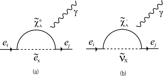
Figure 1: Feynman diagrams which contribute to the branching ratio of $e_{i}\rightarrow e_{j}+\gamma$. There are two types of diagrams, (a) neutralino-slepton loop and (b) chargino-sneutrino loop.

We calculate the branching ratio using (3.2) and the formulas in Appendix C. In order to clarify parameter dependence, let us present an approximate estimation. The decay amplitude is approximated as

$$|A^{{\scriptscriptstyle R}}|^{2}\simeq\frac{\alpha_{2}^{2}}{16\pi^{2}}\frac{|(\bigtriangleup{\bf m}_{\tilde{{\scriptscriptstyle L}}}^{2})_{ij}|^{2}}{m_{{\scriptscriptstyle S}}^{8}}\tan^{2}\beta\ ,$$ (3.3)

where $\alpha_{2}$ is the gauge coupling constant of $SU(2)_{L}$ and $m_{S}$ is a SUSY particle mass. The RGE’s develop the off-diagonal elements of the slepton mass matrix and A-term. These terms at the low energy are approximated as

$$(\bigtriangleup{\bf m}_{\tilde{{\scriptscriptstyle L}}}^{2})_{ij} \simeq -\frac{(6+2a_{0}^{2})m_{0}^{2}}{16\pi^{2}}({\bf Y_{\nu}^{{\dagger}}Y_{\nu}})_{ij}\ln\frac{M_{{\scriptscriptstyle X}}}{M_{{\scriptscriptstyle R}}}\ ,$$ (3.4)

where $M_{{\scriptscriptstyle X}}$ is the GUT scale. Therefore, off-diagonal elements of ${\bf(Y_{\nu}^{{\dagger}}Y_{\nu}})_{ij}$ are the crucial quantity to estimate the branching ratio.

As discussed in section 2, ${\bf(Y_{\nu}^{{\dagger}}Y_{\nu})}_{ij}$ is given by neutrino masses and mixings at the electroweak scale. Therefore, we can compare the quantity ${\bf(Y_{\nu}^{{\dagger}}Y_{\nu})}_{ij}$ among the cases of three neutrino mass spectra: the degenerate, the inverse-hierarchical and the hierarchical masses. In this section, we present numerical results in these three cases. Here, we use eq.(3.2) and the vertex functions in Appendix C for the calculation of the branching ratio including the RGE’s effect.

3.1 $\mu\rightarrow e+\gamma$

We present a qualitative discussion on $({\bf Y}_{\nu}^{{\dagger}}{\bf Y}_{\nu})_{21}$ before predicting the branching ratio BR$(\mu\rightarrow e+\gamma)$. This is given in terms of neutrino masses and mixings at the electroweak scale as follows:

$$({\bf Y}_{\nu}^{{\dagger}}{\bf Y}_{\nu})_{21}=\frac{M_{{\scriptscriptstyle R}}}{v_{u}^{2}}\left[U_{\mu 2}U_{e2}^{*}(m_{\nu 2}-m_{\nu 1})+U_{\mu 3}U_{e3}^{*}(m_{\nu 3}-m_{\nu 1})\right]\ ,$$ (3.5)

where $v_{u}\equiv v\sin\beta$ with $v=174{\rm GeV}$ is taken as an usual notation and the unitarity condition of the lepton mixing matrix elements is used. Taking the three cases of the neutrino mass spectra: the degenerate, the inverse-hierarchical and the normal hierarchical masses, one obtains the following forms, repectively,

$$({\bf Y}_{\nu}^{{\dagger}}{\bf Y}_{\nu})_{21}\simeq \frac{M_{{\scriptscriptstyle R}}}{\sqrt{2}v_{u}^{2}}\frac{\Delta m^{2}_{\rm atm}}{2m_{\nu}}\left[\frac{1}{\sqrt{2}}U_{e2}^{*}\frac{\Delta m_{\odot}^{2}}{\Delta m^{2}_{\rm atm}}+U_{e3}^{*}\right]\ ,\quad({\rm Degenerate})$$

$$\simeq \frac{M_{{\scriptscriptstyle R}}}{\sqrt{2}v_{u}^{2}}\sqrt{\Delta m_{\rm atm}^{2}}\left[\frac{1}{2\sqrt{2}}U_{e2}^{*}\frac{\Delta m_{\odot}^{2}}{\Delta m^{2}_{\rm atm}}-U_{e3}^{*}\right]\ ,\quad({\rm Inverse})$$ (3.6)

$$\simeq \frac{M_{{\scriptscriptstyle R}}}{\sqrt{2}v_{u}^{2}}\sqrt{\Delta m_{\rm atm}^{2}}\left[\frac{1}{\sqrt{2}}U_{e2}^{*}\sqrt{\frac{\Delta m_{\odot}^{2}}{\Delta m^{2}_{\rm atm}}}+U_{e3}^{*}\right]\ ,\quad({\rm Hierarchy})$$

where we take the maximal mixing for the atmospheric neutrinos. Since $U_{e2}\simeq 1/\sqrt{2}$ for the bi-maximal mixing matrix, the first terms in the square brackets of the right hand sides of eqs.(3.6) can be estimated by putting the experimental data. For the case of the degenerate neutrino masses, $({\bf Y}_{\nu}^{{\dagger}}{\bf Y}_{\nu})_{21}$ depends on the unknown neutrino mass scale $m_{\nu}$. As one takes the smaller $m_{\nu}$, one predicts the larger branching ratio. In our calculation, we take $m_{\nu}=0.3{\rm eV}$ , which is close to the upper bound from the neutrinoless double beta decay experiment [25], and also leads to the smallest branching ratio.

We also note that the degenerate case gives the smallest branching ratio BR$(\mu\rightarrow e+\gamma)$ among the three cases as seen in eqs.(3.6) owing to the scale of $m_{\nu}$. It is easy to see the fact that the second terms in eqs.(3.6) are dominant as far as $U_{e3}~{}{\stackrel{{\scriptstyle>}}{{\scriptstyle\sim}}}~{}0.01({\rm degenerate}),~{}0.01({\rm inverse})$ and $0.07({\rm hierarchy})$, respectively. The magnitude and the phase of $U_{e3}$ are important in the comparison between cases of the inverse-hierarchical and the normal hierarchical masses. In the limit of $U_{e3}=0$, the predicted branching ratio in the case of the normal hierarchical masses is larger than the other one. However, for $U_{e3}\simeq 0.2$ the predicted branching ratios are almost the same in both cases.

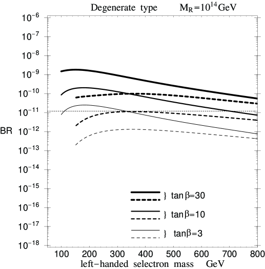
Figure 2: Predicted branching ratio BR$(\mu\rightarrow e+\gamma)$ versus the left-handed selectron mass for $\tan\beta=3,\ 10,\ 30$ in the case of the degenerate neutrino masses. Here $M_{\scriptscriptstyle R}=10^{14}{\rm GeV}$ and $U_{e3}=0.2$ are taken. The solid curves correspond to $M_{2}=150{\rm GeV}$ and the dashed ones to $M_{2}=300{\rm GeV}$. A horizontal dotted line denotes the experimental upper bound.

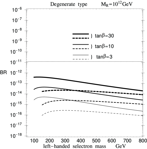
Figure 3: Predicted branching ratio BR$(\mu\rightarrow e+\gamma)$ versus the left-handed selectron mass for $\tan\beta=3,\ 10,\ 30$ in the case of the degenerate neutrino masses. Here $M_{\scriptscriptstyle R}=10^{12}{\rm GeV}$ and $U_{e3}=0.2$ are taken. The solid curves correspond to $M_{2}=150{\rm GeV}$ and the dashed ones to $M_{2}=300{\rm GeV}$.

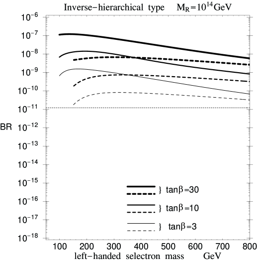
Figure 4: Predicted branching ratio BR$(\mu\rightarrow e+\gamma)$ versus the left-handed selectron mass for $\tan\beta=3,\ 10,\ 30$ in the case of the inverse-hierarchical neutrino masses. Here $M_{\scriptscriptstyle R}=10^{14}{\rm GeV}$ and $U_{e3}=0.2$ are taken. The solid curves correspond to $M_{2}=150{\rm GeV}$ and the dashed ones to $M_{2}=300{\rm GeV}$.

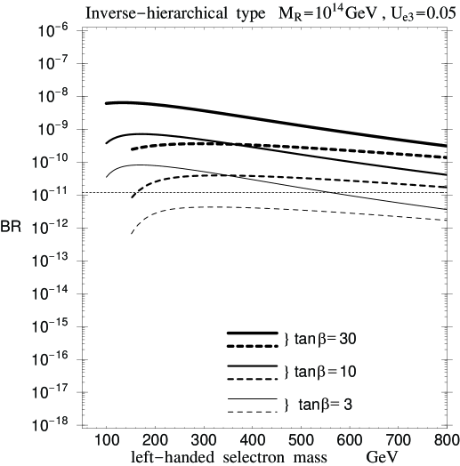
Figure 5: Predicted branching ratio BR$(\mu\rightarrow e+\gamma)$ versus the left-handed selectron mass for $\tan\beta=3,\ 10,\ 30$ in the case of the inverse-hierarchical neutrino masses. Here $M_{\scriptscriptstyle R}=10^{14}{\rm GeV}$ and $U_{e3}=0.05$ are taken. The solid curves correspond to $M_{2}=150{\rm GeV}$ and the dashed ones to $M_{2}=300{\rm GeV}$.

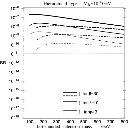
Figure 6: Predicted branching ratio BR$(\mu\rightarrow e+\gamma)$ versus the left-handed selectron mass for $\tan\beta=3,\ 10,\ 30$ in the case of the hierarchical neutrino masses. Here $M_{\scriptscriptstyle R}=10^{14}{\rm GeV}$ and $U_{e3}=0.2$ are taken. The solid curves correspond to $M_{2}=150{\rm GeV}$ and the dashed ones to $M_{2}=300{\rm GeV}$.

At first, we present numerical results in the case of the degenerate neutrino masses assuming ${\bf M_{\scriptscriptstyle R}}=M_{\scriptscriptstyle R}{\bf 1}$. The magnitude of $M_{\scriptscriptstyle R}$ is constained considerably if we impose the $b-\tau$ unfication of Yukawa couplings [26]. In the case of $\tan\beta\leq 30$, the lower bound of $M_{\scriptscriptstyle R}$ is approximately $10^{12}{\rm GeV}$. We take also $M_{\scriptscriptstyle R}\leq 10^{14}{\rm GeV}$, in order that neutrino Yukawa couplings remain below ${\cal O}(1)$. Therefore, we use $M_{\scriptscriptstyle R}=10^{12},\ 10^{14}{\rm GeV}$ in our following calculation.

We take a universal scalar mass $(m_{0})$ for all scalars and $a_{0}=0$ as a universal A-term at the GUT scale ($M_{\scriptscriptstyle X}=2\times 10^{16}$ GeV). The branching ratio of $\mu\rightarrow e+\gamma$ is given versus the left-handed selectron mass $m_{\tilde{e}_{\scriptscriptstyle L}}$ for each $\tan\beta=3,\ 10,\ 30$ and a fixed wino mass $M_{2}$ at the electroweak scale. In fig.2, the branching ratios are shown for $M_{2}=150,\ 300\ {\rm GeV}$ in the case of $U_{e3}=0.2$ with $M_{R}=10^{14}{\rm GeV}$ and $m_{\nu}=0.3$eV, in which the solid curves correspond to $M_{2}=150{\rm GeV}$ and the dashed ones to $M_{2}=300{\rm GeV}$. The threshold of the selectron mass is determined by the recent LEP2 data [27] for $M_{2}=150{\rm GeV}$, however, for $M_{2}=300{\rm GeV}$, determined by the constraint that the left-handed slepton should be heavier than the neutralinos. As the $\tan\beta$ increases, the branching ratio increases because the decay amplitude from the SUSY diagrams is approximately proportional to $\tan\beta$ [7]. It is found that the branching ratio is almost larger than the experimental upper bound in the case of $M_{2}=150{\rm GeV}$. On the other hand, the predicted values are smaller than the experimental bound except for $\tan\beta=30$ in the case of $M_{2}=300{\rm GeV}$.

Our predictions depend on $M_{\scriptscriptstyle R}$ strongly, because the magnitude of the neutrino Yukawa coupling is determined by $M_{\scriptscriptstyle R}$ as seen in eq.(2.5). If $M_{\scriptscriptstyle R}$ reduces to $10^{12}{\rm GeV}$, the branching ratio becomes $10^{4}$ times smaller since it is proportional to $M_{\scriptscriptstyle R}^{2}$. The numerical result is shown in fig.3. We will examine a model [28, 29], which gives the degenerate neutrino masses with $U_{e3}\sim 0.05$ in section 4.

Next we show results in the case of the inverse-hierarchical neutrino masses. As expected in eq.(3.6), the branching ratio is much larger than the one in the degenerate case. In fig.4, the branching ratio is shown for $M_{2}=150,\ 300\ {\rm GeV}$ in the case of $U_{e3}=0.2$ with $M_{\scriptscriptstyle R}=10^{14}{\rm GeV}$. In fig.5, the branching ratio is shown for $U_{e3}=0.05$ with $M_{\scriptscriptstyle R}=10^{14}{\rm GeV}$. The $M_{R}$ dependence is the same as the case of the quasi-degenerate neutrino masses. The predictions almost exceed the experimental bound as far as $U_{e3}\geq 0.05$, $\tan\beta\geq 10$ and $M_{\scriptscriptstyle R}\simeq 10^{14}{\rm GeV}$. This result is based on the assumption ${\bf M}_{\bf{\scriptscriptstyle R}}=M_{{\scriptscriptstyle R}}{\bf 1}$, however, it is not guaranteed in the case of the inverse-hierarchical neutrino masses. We will examine a typical model [30], which gives ${\bf M}_{\bf{\scriptscriptstyle R}}\not=M_{{\scriptscriptstyle R}}{\bf 1}$ in section 4.

For comparison, we show the branching ratio in the case of the hierarchical neutrino masses in fig.6. It is similar to the case of the inverse-hierarchical neutrino masses. The branching ratio in the case of the degenerate neutrino masses is $10^{2}$ times smaller than the one in the inverse-hierarchical and the hierarchical neutrino spectra.

In our numerical analyses we assumed $a_{0}=0$ at the GUT scale $M_{{\scriptscriptstyle X}}$ for simplicity. Let us comment on the A-term dependence, namely $a_{0}\neq 0$ at $M_{{\scriptscriptstyle X}}$. We estimate the branching ratio for $a_{0}=\pm 1$ at $M_{{\scriptscriptstyle X}}$ $({\bf A}={\bf Y}a_{0}m_{0})$. In the degenerate type, the predicted branching ratio is 1.02($a_{0}=1$), 1.07($a_{0}=-1$) times as large as the one in the case of $a_{0}=0$ (tan$\beta=30$, $U_{e3}=0.2$). In the inverse-hierarchical type, the predicted branching ratios are 1.56($a_{0}=1$), 1.54($a_{0}=-1$) times as large as the one in the case of $a_{0}=0$ (tan$\beta=30$, $U_{e3}=0.2$). Therefore the A-term dependence is insignificant in our analyses.

In our calculations, we use the universality condition at $M_{{\scriptscriptstyle X}}$. We also examine the no-scale condition $m_{0}=0$ at $M_{{\scriptscriptstyle X}}$. It is found that the predicted branching ratio is $10$ times smaller than the one in the case of non-zero universal scalar mass.

3.2 Non-degeneracy Effect of ${\bf M}_{R}$

The analyses in the previous section depend on the assumption of $M_{{\scriptscriptstyle R}1}=M_{{\scriptscriptstyle R}2}=M_{{\scriptscriptstyle R}3}\equiv M_{R}$. In the case of the quasi-degenarate neutrino masses in eq.(2.12) this complete degeneracy of ${\bf M}_{{\scriptscriptstyle R}}$ may be deviated in the following magnitude without fine-tuning:

$$\frac{M_{{\scriptscriptstyle R}3}^{2}}{M_{{\scriptscriptstyle R}1}^{2}}\simeq 1\pm\frac{\Delta m_{\rm atm}^{2}}{m_{\nu}^{2}}\ ,\qquad\frac{M_{{\scriptscriptstyle R}2}^{2}}{M_{{\scriptscriptstyle R}1}^{2}}\simeq 1\pm\frac{\Delta m_{\odot}^{2}}{m_{\nu}^{2}}\ .$$ (3.7)

Therefore, we parametrize $M_{{\scriptscriptstyle R}}$ as

$${\bf M_{{\scriptscriptstyle R}}}=M_{{\scriptscriptstyle R}}\left(\begin{array}[]{ccc}1&0&0\\ 0&1+\varepsilon_{2}&0\\ 0&0&1+\varepsilon_{3}\end{array}\right)\ ,$$ (3.11)

where $\varepsilon_{2}\simeq\Delta m_{\odot}^{2}/2m_{\nu}^{2}$ and $\varepsilon_{3}\simeq\Delta m_{\rm atm}^{2}/2m_{\nu}^{2}$. By using eq.(2.6), we obtain

$${\bf Y}^{\dagger}_{\nu}{\bf Y}_{\nu}=\frac{M_{{\scriptscriptstyle R}}}{v^{2}_{u}}{\bf U}_{{\rm{\scriptscriptstyle M}{\scriptscriptstyle N}{\scriptscriptstyle S}}}\left(\begin{array}[]{ccc}\sqrt{m_{\nu 1}}&0&0\\ 0&\sqrt{m_{\nu 2}}&0\\ 0&0&\sqrt{m_{\nu 3}}\end{array}\right){\bf K}\left(\begin{array}[]{ccc}\sqrt{m_{\nu 1}}&0&0\\ 0&\sqrt{m_{\nu 2}}&0\\ 0&0&\sqrt{m_{\nu 3}}\end{array}\right){\bf U}^{\rm T}_{{\rm{\scriptscriptstyle M}{\scriptscriptstyle N}{\scriptscriptstyle S}}}\ ,$$ (3.12)

where

$${\bf K}\equiv{\bf R}^{\dagger}\left(\begin{array}[]{ccc}1&0&0\\ 0&1+\varepsilon_{2}&0\\ 0&0&1+\varepsilon_{3}\end{array}\right){\bf R}\ .$$ (3.13)

Then, we have

$$({\bf Y}^{\dagger}_{\nu}{\bf Y}_{\nu})_{21}=\frac{M_{{\scriptscriptstyle R}}}{v^{2}_{u}}\sum^{3}_{i,j}U_{2i}U_{1j}(K_{ij}\sqrt{m_{\nu i}}\sqrt{m_{\nu j}})\ ,$$ (3.14)

with

$$K_{ij}=\delta_{ij}+\varepsilon_{2}R_{2i}R_{2j}+\varepsilon_{3}R_{3i}R_{3j}\ ,$$ (3.15)

where we used ${\bf R}^{\rm T}{\bf R=1}$ . So, we get

$$({\bf Y}^{\dagger}_{\nu}{\bf Y}_{\nu})_{21}=\left.({\bf Y}^{\dagger}_{\nu}{\bf Y}_{\nu})_{21}\right|_{\bf M_{{\scriptscriptstyle R}\propto 1}}+\Delta({\bf Y}^{\dagger}_{\nu}{\bf Y}_{\nu})_{21}\ ,$$ (3.16)

where the first term is the $({\bf Y}^{\dagger}_{\nu}{\bf Y}_{\nu})_{21}$ element in eq.(3.5), which corresponds to the ${\bf M_{{\scriptscriptstyle R}\propto 1}}$, while the second term stands for the deviation from it as follows:

$$\Delta({\bf Y}^{\dagger}_{\nu}{\bf Y}_{\nu})_{21}=\frac{M_{{\scriptscriptstyle R}}}{v^{2}_{u}}\sum^{3}_{i,j}U_{2i}U_{1j}\sqrt{m_{\nu i}}\sqrt{m_{\nu j}}(\varepsilon_{2}R_{2i}R_{2j}+\varepsilon_{3}R_{3i}R_{3j})\ .$$ (3.17)

In order to estimate the second term, we use $\varepsilon_{2}=0.0001$ and $\varepsilon_{3}=0.01$ taking account of $\varepsilon_{2}\simeq\Delta m_{\odot}^{2}/2m_{\nu}^{2}$ and $\varepsilon_{3}\simeq\Delta m_{\rm atm}^{2}/2m_{\nu}^{2}$, where $m_{\nu}=0.3{\rm eV}$ is put. Since $m_{\nu i}\simeq m_{\nu j}$ and $R_{ij}\leq 1$, we get

$$\Delta({\bf Y}^{\dagger}_{\nu}{\bf Y}_{\nu})_{21} \sim \frac{M_{{\scriptscriptstyle R}}}{v^{2}_{u}}\sum^{3}_{i,j}U_{2i}U_{1j}m_{\nu}\varepsilon_{3}R_{3i}R_{3j}$$ (3.18)

$$\leq \frac{M_{{\scriptscriptstyle R}}}{v^{2}_{u}}\frac{1}{2\sqrt{2}}m_{\nu}\varepsilon_{3}\sim 3.5\times 10^{-3}\ .$$

Taking this maximal value, we can estimate the branching ratio as follows:

$$\frac{BR({\rm non\mbox{-}degenerate}\ M_{{\scriptscriptstyle R}})}{BR({\rm degenerate}\ M_{{\scriptscriptstyle R}})}\leq\left(\frac{2.6+3.5}{2.6}\right)^{2}\simeq 5.5\ .$$ (3.19)

Therefore, the enhancement due to the second term is at most factor 5. This conclusion does not depend on the specific form of ${\bf R}$

Consider the case of the inverse-hierarchical type of neutrino masses. We take $\varepsilon_{2}\sim 0.01$ with the similar argument of the quasi-degenerate type neutrino masses, because $m_{\nu 1}$ and $m_{\nu 2}$ are almost degenerate and $\varepsilon_{2}\simeq\Delta m_{\odot}^{2}/2\Delta m_{\rm atm}^{2}$ in this case. Then, we get

$$\Delta({\bf Y}^{\dagger}_{\nu}{\bf Y}_{\nu})_{21} = \frac{M_{{\scriptscriptstyle R}}}{v^{2}_{u}}\sum^{2}_{i,j}U_{2i}U_{1j}m_{\nu 1}\varepsilon_{2}R_{2i}R_{2j}$$ (3.20)

$$\leq \frac{M_{{\scriptscriptstyle R}}}{v^{2}_{u}}\frac{1}{2\sqrt{2}}m_{\nu 1}\varepsilon_{2}\sim 0.063\times 10^{-2}\ ,$$

where we assume $\varepsilon_{2}\geq\varepsilon_{3}$ and use $m_{\nu 3}\simeq 0$, $m_{\nu 1}\simeq m_{\nu 2}\simeq 0.054$eV and $R_{ij}\leq 1$. Taking the maximal value, we get

$$\frac{BR({\rm non\mbox{-}degenerate}\ M_{{\scriptscriptstyle R}})}{BR({\rm degenerate}\ M_{{\scriptscriptstyle R}})}\leq\left(\frac{2.7+0.063}{2.7}\right)^{2}\simeq 1.04\ .$$ (3.21)

Thus, the effect of the $\Delta({\bf Y}^{\dagger}_{\nu}{\bf Y}_{\nu})_{21}$ is very small in the case of the inverse hierarchical neutrino masses.

These discussions in this subsection are also available qualitatively for the $\tau\rightarrow\mu+\gamma$ process.

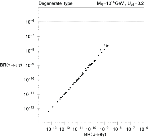
Figure 7: Predicted branching ratio BR$(\tau\rightarrow\mu+\gamma)$ versus BR$(\mu\rightarrow e+\gamma)$ for $\tan\beta=3,\ 10,\ 30$ in the case of the degenerate neutrino masses. Here $M_{\scriptscriptstyle R}=10^{14}{\rm GeV}$, $m_{\nu}=0.3$eV and $U_{e3}=0.2$ are taken and the left-handed selectron mass is taken as same as in figs.2-4.

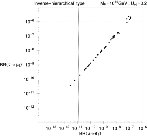
Figure 8: Predicted branching ratio BR$(\tau\rightarrow\mu+\gamma)$ versus BR$(\mu\rightarrow e+\gamma)$ for $\tan\beta=3,\ 10,\ 30$ in the case of the inverse-hierarchical neutrino masses. Here $M_{\scriptscriptstyle R}=10^{14}{\rm GeV}$ and $U_{e3}=0.2$ are taken and the left-handed selectron mass is taken as same as in figs.2-4.

3.3 $\tau\rightarrow\mu+\gamma$

Let us study the $\tau\rightarrow\mu+\gamma$ process. In this case, we should discuss

$$({\bf Y}_{\nu}^{{\dagger}}{\bf Y}_{\nu})_{32}=\frac{M_{{\scriptscriptstyle R}}}{v_{u}^{2}}\left[U_{\tau 2}U_{\mu 2}^{*}(m_{\nu 2}-m_{\nu 1})+U_{\tau 3}U_{\mu 3}^{*}(m_{\nu 3}-m_{\nu 1})\right]\ .$$ (3.22)

It should be stressed that it is independent of $U_{e3}$ in contrast to $({\bf Y}_{\nu}^{\dagger}{\bf Y}_{\nu})_{21}$. Therefore we can determine the following form of $({\bf Y}_{\nu}^{\dagger}{\bf Y}_{\nu})_{32}$ at the electroweak scale by using the bi-maximal mixing matrix:

$$({\bf Y}_{\nu}^{{\dagger}}{\bf Y}_{\nu})_{32}\simeq \frac{M_{{\scriptscriptstyle R}}}{v_{u}^{2}}\left[-\frac{1}{4}\frac{\Delta m_{\odot}^{2}}{2m_{\nu}}+\frac{1}{2}\frac{\Delta m^{2}_{\rm atm}}{2m_{\nu}}\right]\ \simeq\frac{M_{{\scriptscriptstyle R}}}{4v_{u}^{2}}\frac{\Delta m^{2}_{\rm atm}}{m_{\nu}}\quad,\ ({\rm Degenerate})$$

$$\simeq \frac{M_{{\scriptscriptstyle R}}}{v_{u}^{2}}\left[\frac{1}{8}\frac{\Delta m_{\odot}^{2}}{\sqrt{\Delta m^{2}_{\rm atm}}}-\frac{1}{2}\sqrt{\Delta m^{2}_{\rm atm}}\right]\ \simeq-\frac{M_{{\scriptscriptstyle R}}}{2v_{u}^{2}}\sqrt{\Delta m^{2}_{\rm atm}}\quad,\ ({\rm Inverse})$$

$$\simeq \frac{M_{{\scriptscriptstyle R}}}{v_{u}^{2}}\left[-\frac{1}{4}\sqrt{\Delta m_{\odot}^{2}}+\frac{1}{2}\sqrt{\Delta m^{2}_{\rm atm}}\right]\ \simeq\frac{M_{{\scriptscriptstyle R}}}{2v_{u}^{2}}\sqrt{\Delta m^{2}_{\rm atm}}\quad.\ ({\rm Hierarchy})$$

We see that the case of the inverse-hierarchical masses and the hierarchical masses are almost the same as seen in eqs.(LABEL:mass3).

Let us present numerical results of BR$(\tau\rightarrow\mu+\gamma)$ [31] versus BR$(\mu\rightarrow e+\gamma)$ [11] in the case of the degenerate neutrino mass, in which $\tan\beta=3,\ 10,\ 30$ are taken. In fig.7, the branching ratio is plotted for $M_{2}=150,\ 300\ {\rm GeV}$ for $U_{e3}=0.2$ with $M_{\scriptscriptstyle R}=10^{14}{\rm GeV}$. Dotted lines are the experimantal upper bounds for BR$(\tau\rightarrow\mu+\gamma)$ and BR$(\mu\rightarrow e+\gamma)$, respectively. The dependence of $\tan\beta$ is the same as the case of $\mu\rightarrow e+\gamma$. It is found that the branching ratio is completely smaller than the experimental upper bound in the case of $\tau\rightarrow\mu+\gamma$ in contrast with the case of $\mu\rightarrow e+\gamma$.

Next we show the results in the case of the inverse-hierarchical neutrino masses. As expected in eqs.(LABEL:mass3), the branching ratio is much larger than the one in the degenerate case. In fig.8, the branching ratio is shown for $M_{2}=150,\ 300\ {\rm GeV}$ in the case of $U_{e3}=0.2$ with $M_{\scriptscriptstyle R}=10^{14}{\rm GeV}$. In conclusion, the predicted branching ratio is larger than the one in the case of the degenerate neutrino mass, and it is almost smaller than the experimental upper bound for $\tau\rightarrow\mu+\gamma$ in contrast with $\mu\rightarrow e+\gamma$. The constraint of BR$(\mu\rightarrow e+\gamma)$ is always severer than the one in the case of BR$(\tau\rightarrow\mu+\gamma)$.

4 Typical models and numerical analyses

4.1 $S_{3{\scriptscriptstyle L}}\times S_{3{\scriptscriptstyle R}}$ flavor symmetry model - Degenarate type

In this section we examine the neutrino model proposed by Fukugida, Tanimoto and Yanagida [28], which derives the quasi-degenerate masses, $m_{\nu 1}\sim m_{\nu 2}\sim m_{\nu 3}$. This model is based on the $S_{3{\scriptscriptstyle L}}\times S_{3{\scriptscriptstyle R}}$ flavor symmetry [32]. Taking ${\bf M_{\scriptscriptstyle R}}=M_{\scriptscriptstyle R}{\bf 1}$, the neutrino Yukawa coupling is given as follows:

$${\bf Y}_{\nu}=Y_{\nu 0}\left[\left(\begin{array}[]{ccc}1&0&0\\ 0&1&0\\ 0&0&1\end{array}\right)+\left(\begin{array}[]{ccc}0&0&0\\ 0&\epsilon_{\nu}&0\\ 0&0&\delta_{\nu}\end{array}\right)\right]\ ,$$ (4.7)

where we take the diagonal basis for the neutrino sector. The first matrix is the $S_{3{\scriptscriptstyle L}}$ invariant one, and the second one is the symmetry breaking term. The parameters $Y_{\nu 0},\epsilon_{\nu}$ and $\delta_{\nu}$ are constrained by the experimental values of $\Delta m_{\rm atm}^{2}$ and $\Delta m_{\odot}^{2}$. Therefore, the flavor mixings come from the charged lepton Yukawa couplings.

The charged lepton Yukawa coupling is given by the symmetry breaking parameters $\epsilon_{l},\delta_{l}$ as follows:

$${\bf Y}_{e}=Y_{e0}\left[\left(\begin{array}[]{ccc}1&1&1\\ 1&1&1\\ 1&1&1\end{array}\right)+\left(\begin{array}[]{ccc}-\epsilon_{l}&0&0\\ 0&+\epsilon_{l}&0\\ 0&0&+\delta_{l}\end{array}\right)\right]\ .$$ (4.14)

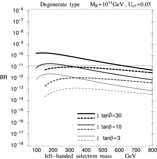
Figure 9: Predicted branching ratio BR$(\mu\rightarrow e+\gamma)$ versus the left-handed selectron mass for $\tan\beta=3,\ 10,\ 30$ in the case of the $S_{3L}\times S_{3R}$ flavor symmetry model. Here $M_{\scriptscriptstyle R}=10^{14}{\rm GeV}$ are taken. The solid curves correspond to $M_{2}=150{\rm GeV}$ and the dashed ones to $M_{2}=300{\rm GeV}$.

Since $Y_{e0},\epsilon_{l}$ and $\delta_{l}$ are fixed by the charged lepton masses, one gets the lepton mixing matrix elements as follows :

$${\bf U}_{{\rm{\scriptscriptstyle M}{\scriptscriptstyle N}{\scriptscriptstyle S}}}\simeq\left(\begin{array}[]{ccc}1/\sqrt{2}&-1/\sqrt{2}&\sqrt{2/3}\sqrt{m_{e}/m_{\mu}}\\ 1/\sqrt{6}&1/\sqrt{6}&-2/\sqrt{6}\\ 1/\sqrt{3}&1/\sqrt{3}&1/\sqrt{3}\end{array}\right)~{}\ .$$ (4.18)

As a result, we see $U_{e3}=\sqrt{2/3}\sqrt{m_{e}/m_{\mu}}\sim 0.05$ from eq.(4.18).

We estimated the branching ratio of the processes $\mu\rightarrow e+\gamma$ and $\tau\rightarrow\mu+\gamma$ by using $U_{e3}=0.05$. We show the branching ratio for $M_{2}=150$ GeV and $300$GeV taking tan$\beta=3,10,30$ in fig.9. Because of the smallness of $U_{e3}$, we see that BR$(\mu\rightarrow e+\gamma)$ is smaller than the experimental upper bound except for tan$\beta=30$, and $M_{2}=150$GeV.

We have also estimated the branching ratio BR($\tau\rightarrow\mu+\gamma)$ for tan$\beta=30$, which is much smaller than the experimental bound BR($\tau\rightarrow\mu+\gamma)<1.1\times 10^{-6}$. Thus, the $\mu\rightarrow e+\gamma$ process provides the severe constraint compared with the $\tau\rightarrow\mu+\gamma$ in the present experimental situation.

4.2 The Shafi-Tavartkiladze model - Inverse-hierarchical type

The typical model of the inverse-hierarchical neutrino masses is the Zee model [33], in which the right-handed neutrinos do not exist. However, one can also consider a Yukawa texture which leads to the inverse-hierarchical masses through the see-saw mechanism, namely the Shafi-Tavartkiladze model [30].

Shafi and Tavartkiladze utilize the anomalous $U(1)$ flavor symmetry [34]. In this model, due to the Froggatt-Nielsen mechanism [35], one of the Yukawa interaction term in the effective theory is given as

$$e^{c}_{{{\scriptscriptstyle R}}i}L_{j}H_{d}\left(\frac{S}{M_{\rm pl}}\right)^{m_{ij}}\ ,$$ (4.19)

where $e^{c}_{{\scriptscriptstyle R}{i}}$ and $L_{j}$ are the right-handed charged lepton and the left-handed lepton doublet, respectively, $H_{d}$ is Higgs doublet, and $S$ is singlet field. The effective Yukawa couplings are given in terms of

$$\lambda\equiv\frac{\langle S\rangle}{M_{\rm pl}}\simeq 0.2\ .$$ (4.20)

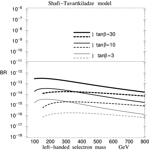
Figure 10: Predicted branching ratio BR$(\mu\rightarrow e+\gamma)$ versus the left-handed selectron mass for $\tan\beta=3,\ 10,\ 30$ in the case of the Shafi-Tavartkiladze model[30]. The solid curves correspond to $M_{2}=150{\rm GeV}$ and the dashed ones to $M_{2}=300{\rm GeV}$.

The neutrino mass matrix is given in Appendix D. Fixing the $U(1)$ flavor charges $k$, $n$, $k^{{}^{\prime}}$ as $k$=0, $n$=2, $k^{{}^{\prime}}$=2, which is consistent with neutrino mass data, the Yukawa coupling is given as

$${\bf Y}_{\nu} = \left(\begin{array}[]{ccc}\lambda^{4}&\lambda^{2}&\lambda^{2}\\ 1&0&0\end{array}\right)\ ,$$ (4.23)

and the right-handed neutrino Majorana mass matrix is given as

$${\bf M}_{\bf{\scriptscriptstyle R}} = M_{{\scriptscriptstyle R}}\left(\begin{array}[]{cc}\lambda^{4}&1\\ 1&0\end{array}\right)\ .$$ (4.26)

It is remarked that right-handed neutrinos contain only two generations in this model. In eq.(4.23), components 2-2 and 2-3 must be zero for the sake of holomorphy of superpotential, it is called SUSY zero. The neutrino mass matrix is given by the see-saw mechanism as

$${\bf m}_{\nu}={\bf Y}_{\nu}^{\rm T}{\bf M}_{\bf{\scriptscriptstyle R}}^{-1}{\bf Y}_{\nu}v_{u}^{2}=\frac{\lambda^{2}v_{u}^{2}}{M_{{\scriptscriptstyle R}}}\left(\begin{array}[]{ccc}\lambda^{2}&1&1\\ 1&0&0\\ 1&0&0\end{array}\right)\ ,$$ (4.30)

where the order one coefficient in front of each entry is neglected. This mass matrix gives the inverse-hierarchical neutrino masses. The ${\bf Y}_{\nu}^{{\dagger}}{\bf Y}_{\nu}$ is given as

$${\bf Y}_{\nu}^{{\dagger}}{\bf Y}_{\nu}=\left(\begin{array}[]{ccc}1+\lambda^{8}&\lambda^{6}&\lambda^{6}\\ \lambda^{6}&\lambda^{4}&\lambda^{4}\\ \lambda^{6}&\lambda^{4}&\lambda^{4}\\ \end{array}\right)\ .$$ (4.34)

It is noticed that the component $({\bf Y}_{\nu}^{{\dagger}}{\bf Y}_{\nu})_{21}$ is suppressed as

$$({\bf Y}_{\nu}^{{\dagger}}{\bf Y}_{\nu})_{21}\sim\l^{6}\sim{\cal O}(10^{-5})\ .$$ (4.35)

Then, we expect that the branching ratio of $\mu\rightarrow e+\gamma$ in this model is much smaller than the one in the case of $({\bf M}_{\bf{\scriptscriptstyle R}})_{3\times 3}=M_{{\scriptscriptstyle R}}({\bf 1})_{3\times 3}$ in section 3.

In fig.10, the branching ratio is shown for $M_{2}=150,\ 300\ {\rm GeV}$. The predictions are given by taking $\lambda=0.2$ and all of order one coefficients in the Yukawa couplings are fixed to be one. The predicted value is much smaller than the one in the inverse-hierarchical case discussed in the section 3. Because $({\bf Y}_{\nu}^{{\dagger}}{\bf Y}_{\nu})_{21}$ is proportional to $\l^{6}$, the smallness of the branching ratio is understandable.

5 Summary and Discussions

We have investigated the lepton flavor violating processes $\mu\rightarrow e+\gamma$ and $\tau\rightarrow\mu+\gamma$, in the framework of the MSSM with the right-handed neutrinos. Even if we impose the universality condition for the soft scalar masses and A-terms at the GUT scale, off-diagonal elements of the left-handed slepton mass matrix are generated through the RGE’s running effects from the GUT scale to the right-handed neutrino mass scale $M_{{\scriptscriptstyle R}}$. We have taken the LMA-MSW solution for the neutrino masses and mixings.

The branching ratios of $\mu\rightarrow e+\gamma$ and $\tau\rightarrow\mu+\gamma$ processes are proportional to ${\bf|(Y_{\nu}^{{\dagger}}Y_{\nu})}_{ij}|^{2}$. Since ${\bf(Y_{\nu}^{{\dagger}}Y_{\nu})}_{ij}$ depends on the mass spectrum of neutrinos, we can compare the branching ratio of three cases of neutrino mass spectra: the degenerate, the inverse-hierarchical and the hierarchical case.

First, we have studied the three types in the case of $\mu\rightarrow e+\gamma$, in which we take ${\bf M}_{\bf{\scriptscriptstyle R}}=M_{{\scriptscriptstyle R}}{\bf 1}$. For the case of the degenerate neutrino masses, the branching ratio depends on the unknown neutrino mass $m_{\nu}$. We have taken $m_{\nu}=0.3$eV, which gives us the largest branching ratio. It is emphasized that the magnitude of $U_{e3}$ is one of important ingredients to predict BR($\mu\rightarrow e+\gamma$). The branching ratio of the inverse-hierarchical case almost exceeds the experimental upper bound and is much larger than the degenerate case for $M_{2}=150{\rm GeV}$ and $M_{2}=300{\rm GeV}$. In general, we expect the relation BR(degenerate)$\ll$BR(inverse-hierarchical)$<$ BR(hierarchical). The effect of the deviation from ${\bf M}_{\bf{\scriptscriptstyle R}}=M_{{\scriptscriptstyle R}}{\bf 1}$ has been estimated. The enhancement of the branching ratios are at most factor five in the case of the quasi-degenerate neutrino mass spectrum.

Second, we have studied the three cases in $\tau\rightarrow\mu+\gamma$. It is noticed that branching ratio is independent of $U_{e3}$ in contrast to the case of $\mu\rightarrow e+\gamma$. For the degenerate neutrino masses, the branching ratio is completely smaller than the experimental upper bound. For the inverse-hierarchical neutrino masses, the branching ratio is almost smaller than the experimental bound. The constraint of BR$(\mu\rightarrow e+\gamma)$ is always severer than the one in the case of BR$(\tau\rightarrow\mu+\gamma)$.

Finally, we have investigated the branching ratio of $\mu\rightarrow e+\gamma$ in the typical models of the degenetate and the inverse-hierarchical cases. Since the $S_{3{\scriptscriptstyle L}}\times S_{3{\scriptscriptstyle R}}$ model, which is a typical one of the degenerate case, predicts $U_{e3}\simeq 0.05$, the branching ratio is much smaller than the case of $U_{e3}\simeq 0.2$. The Shafi-Tavartkiladze model, which is a typical one of the inverse-hierarchical case, predicts the very small branching ratio. Thus, the models can be tested by the $\mu\rightarrow e+\gamma$ process.

The branching ratio of $\mu\rightarrow e+\gamma$ and $\tau\rightarrow\mu+\gamma$ will be improved to the lebel $10^{-14}$ in the PSI and $10^{-(7-8)}$ in the B factories in KEK and SLAC, respectively. Therefore, future experiments can probe the framework for the neutrino masses.

Acknowledgements
We would like to thank Drs. J. Sato, T. Kobayashi, T. Goto and H. Nakano for useful discussions. We also thank the organizers and participants of Summer Institute 2001 held at Yamanashi, Japan for helpful discussions. This research is supported by the Grant-in-Aid for Science Research, Ministry of Education, Science and Culture, Japan(No.10640274, No.12047220).

Appendix A Yukawa Matrix

The Yukawa matrix is determined in general as follows [10]. The left-handed neutrino mass matrix is given as

$${\bf m_{\nu}}=\left({\bf Y_{\nu}}v_{u}\right)^{\rm T}{\bf M}_{\bf{\scriptscriptstyle R}}^{-1}\left({\bf Y_{\nu}}v_{u}\right)\ ,$$ (A.1)

via the see-saw mechanism, where $v_{u}$ is the vacuum expectation value (VEV) of Higgs $H_{u}$. One can always take the diagonal form of the right-handed Majorana neutrino mass matrix ${\bf M_{\scriptscriptstyle R}}={\bf M_{\scriptscriptstyle R}^{{\scriptscriptstyle\rm diag}}}$. The neutrino mass matrix ${\bf m_{\nu}}$ is diagonalized by a single unitary matrix

$${\bf m_{\nu}^{{\scriptscriptstyle\rm diag}}} \equiv {\bf U}_{{\rm{\scriptscriptstyle M}{\scriptscriptstyle N}{\scriptscriptstyle S}}}^{\rm T}{\bf m_{\nu}}{\bf U_{{\rm{\scriptscriptstyle M}{\scriptscriptstyle N}{\scriptscriptstyle S}}}}\ ,$$ (A.2)

where ${\bf U_{{\rm{\scriptscriptstyle M}{\scriptscriptstyle N}{\scriptscriptstyle S}}}}$ is the MNS matrix. In eqs.(A.1) and (A.2), one can divide ${\bf M_{\scriptscriptstyle R}^{{\scriptscriptstyle\rm diag}}}$ into square roots

$${\bf m_{\nu}^{{\scriptscriptstyle\rm diag}}} = {\bf U}_{{\rm{\scriptscriptstyle M}{\scriptscriptstyle N}{\scriptscriptstyle S}}}^{\rm T}{\bf Y}_{\nu}^{\rm T}\left(\bf{\bf M_{\scriptscriptstyle R}^{{\scriptscriptstyle\rm diag}}}\right)^{-1}{\bf Y_{\nu}U_{{\rm{\scriptscriptstyle M}{\scriptscriptstyle N}{\scriptscriptstyle S}}}}v_{u}^{2}$$ (A.3)

$$= {\bf U}_{{\rm{\scriptscriptstyle M}{\scriptscriptstyle N}{\scriptscriptstyle S}}}^{\rm T}{\bf Y}_{\nu}^{\rm T}\sqrt{\left({\bf M_{\scriptscriptstyle R}^{{\scriptscriptstyle\rm diag}}}\right)^{-1}}\sqrt{\left({\bf M_{\scriptscriptstyle R}^{{\scriptscriptstyle\rm diag}}}\right)^{-1}}{\bf Y_{\nu}}{\bf U_{{\rm{\scriptscriptstyle M}{\scriptscriptstyle N}{\scriptscriptstyle S}}}}v_{u}^{2}\ .$$

Multiplying the inverse square root of the matrix ${\bf m}_{\nu}^{{\scriptscriptstyle\rm diag}}$ from both right and left hand sides of eq.(A.3), one gets the following form

$${\bf 1} = \sqrt{\left({\bf m_{\nu}^{{\scriptscriptstyle\rm diag}}}\right)^{-1}}{\bf U}_{{\rm{\scriptscriptstyle M}{\scriptscriptstyle N}{\scriptscriptstyle S}}}^{\rm T}{\bf Y}_{\nu}^{\rm T}\sqrt{\left({\bf M_{\scriptscriptstyle R}^{{\scriptscriptstyle\rm diag}}}\right)^{-1}}v_{u}^{2}\sqrt{\left({\bf M_{\scriptscriptstyle R}^{{\scriptscriptstyle\rm diag}}}\right)^{-1}}{\bf Y_{\nu}U_{{\rm{\scriptscriptstyle M}{\scriptscriptstyle N}{\scriptscriptstyle S}}}}\sqrt{\left({\bf m_{\nu}^{{\scriptscriptstyle\rm diag}}}\right)^{-1}}$$ (A.4)

$$\equiv {\bf R}^{\rm T}{\bf R}\ ,$$

where one has defined the following complex orthogonal 3$\times$3 matrix

$${\bf R}\equiv v_{u}\sqrt{\left({\bf M_{\scriptscriptstyle R}^{{\scriptscriptstyle\rm diag}}}\right)^{-1}}{\bf Y_{\nu}U_{{\rm{\scriptscriptstyle M}{\scriptscriptstyle N}{\scriptscriptstyle S}}}}\sqrt{\left({\bf m_{\nu}^{{\scriptscriptstyle\rm diag}}}\right)^{-1}},$$ (A.5)

and ${\bf R}$ depends on models. Therefore, one can write the neutrino Yukawa coupling as

$${\bf Y_{\nu}}=\frac{1}{v_{u}}\sqrt{{\bf M_{\scriptscriptstyle R}^{{\scriptscriptstyle\rm diag}}}}\ {\bf R}\ \sqrt{{\bf m_{\nu}^{{\scriptscriptstyle\rm diag}}}}\ {\bf U}^{\rm T}_{{\rm{\scriptscriptstyle M}{\scriptscriptstyle N}{\scriptscriptstyle S}}}\ ,$$ (A.6)

or explicitly

$${\bf Y_{\nu}}=\frac{1}{v_{u}}\left(\matrix{\sqrt{M_{{\scriptscriptstyle R}1}}&0&0\cr 0&\sqrt{M_{{\scriptscriptstyle R}2}}&0\cr 0&0&\sqrt{M_{{\scriptscriptstyle R}3}}\cr}\right){\bf R}\left(\matrix{\sqrt{m_{\nu 1}}&0&0\cr 0&\sqrt{m_{\nu 2}}&0\cr 0&0&\sqrt{m_{\nu 3}}\cr}\right){\bf U}^{\rm T}_{{\rm{\scriptscriptstyle M}{\scriptscriptstyle N}{\scriptscriptstyle S}}}\ .$$ (A.7)

Appendix B RGEs

B.1 From $M_{\rm{\scriptscriptstyle X}}$ to $M_{\rm{\scriptscriptstyle R}}$

$$\mu\frac{d}{d\mu}g^{2}_{i} = \frac{1}{8\pi^{2}}b_{i}g^{4}_{i},~{}~{}~{}(b_{1},b_{2},b_{3})=(\frac{33}{5},1,-3)\ ,$$

$$\mu\frac{d}{d\mu}M_{i} = \frac{b_{i}}{2\pi}\alpha_{i}M_{i}\ ,~{}~{}~{}\alpha_{i}=\frac{g^{2}_{i}}{4\pi}~{}~{}~{}(i=1,2,3)\ ,$$

$$\mu\frac{d}{d\mu}{\bf Y}_{e}^{ij} = \frac{1}{16\pi^{2}}\left[\left\{-\frac{9}{5}g_{1}^{2}-3g_{2}^{2}+3{\rm Tr}({\bf Y}_{d}{\bf Y}_{d}^{\dagger})+{\rm Tr}({\bf Y}_{e}{\bf Y}_{e}^{\dagger})\right\}{\bf Y}_{e}^{ij}\right.$$

$$\left.+3({\bf Y}_{e}{\bf Y}_{e}^{\dagger}{\bf Y}_{e})^{ij}+({\bf Y}_{e}{\bf Y}_{\nu}^{\dagger}{\bf Y}_{\nu})^{ij}\right],$$

$$\mu\frac{d}{d\mu}{\bf Y}_{\nu}^{ij} = \frac{1}{16\pi^{2}}\left[\left\{-\frac{3}{5}g_{1}^{2}-3g_{2}^{2}+3{\rm Tr}({\bf Y}_{u}{\bf Y}_{u}^{\dagger})+{\rm Tr}({\bf Y}_{\nu}{\bf Y}_{\nu}^{\dagger})\right\}{\bf Y}_{\nu}^{ij}\right.$$

$$\left.+3({\bf Y}_{\nu}{\bf Y}_{\nu}^{\dagger}{\bf Y}_{\nu})^{ij}+({\bf Y}_{\nu}{\bf Y}_{e}^{\dagger}{\bf Y}_{e})^{ij}\right],$$

$$\mu\frac{d}{d\mu}{\bf Y}_{u}^{ij} = \frac{1}{16\pi^{2}}\left[\left\{-\frac{13}{15}g_{1}^{2}-3g_{2}^{2}-\frac{16}{3}g_{3}^{2}+3{\rm Tr}({\bf Y}_{u}{\bf Y}_{u}^{\dagger})+{\rm Tr}({\bf Y}_{\nu}{\bf Y}_{\nu}^{\dagger})\right\}{\bf Y}_{u}^{ij}\right.$$

$$\left.+3({\bf Y}_{u}{\bf Y}_{u}^{\dagger}{\bf Y}_{u})^{ij}+({\bf Y}_{u}{\bf Y}_{d}^{\dagger}{\bf Y}_{d})^{ij}\right],$$

$$\mu\frac{d}{d\mu}{\bf Y}_{d}^{ij} = \frac{1}{16\pi^{2}}\left[\left\{-\frac{7}{15}g_{1}^{2}-3g_{2}^{2}-\frac{16}{3}g_{3}^{2}+3{\rm Tr}({\bf Y}_{d}{\bf Y}_{d}^{\dagger})+{\rm Tr}({\bf Y}_{e}{\bf Y}_{e}^{\dagger})\right\}{\bf Y}_{d}^{ij}\right.$$

$$\left.+3({\bf Y}_{d}{\bf Y}_{d}^{\dagger}{\bf Y}_{d})^{ij}+({\bf Y}_{d}{\bf Y}_{u}^{\dagger}{\bf Y}_{u})^{ij}\right],$$

$$\mu\frac{d}{d\mu}({\bf m}^{2}_{\tilde{\scriptscriptstyle L}})_{i}^{j} = \frac{1}{16\pi^{2}}\left[\left({\bf m}^{2}_{\tilde{\scriptscriptstyle L}}{\bf Y}_{e}^{\dagger}{\bf Y}_{e}+{\bf Y}_{e}^{\dagger}{\bf Y}_{e}{\bf m}^{2}_{\tilde{\scriptscriptstyle L}}\right)_{i}^{j}+\left({\bf m}^{2}_{\tilde{\scriptscriptstyle L}}{\bf Y}_{\nu}^{\dagger}{\bf Y}_{\nu}+{\bf Y}_{\nu}^{\dagger}{\bf Y}_{\nu}{\bf m}^{2}_{\tilde{\scriptscriptstyle L}}\right)_{i}^{j}\right.$$

$$+2\left({\bf Y}_{e}^{\dagger}{\bf m}^{2}_{\tilde{e}}{\bf Y}_{e}+m^{2}_{H_{d}}{\bf Y}_{e}^{\dagger}{\bf Y}_{e}+{\bf A}_{e}^{\dagger}{\bf A}_{e}\right)_{i}^{j}$$

$$+2\left({\bf Y}_{\nu}^{\dagger}m^{2}_{\tilde{\nu}}{\bf Y}_{\nu}+{m}^{2}_{H_{u}}{\bf Y}_{\nu}^{\dagger}{\bf Y}_{\nu}+{\bf A}_{\nu}^{\dagger}{\bf A}_{\nu}\right)_{i}^{j}$$

$$\left.-\left(\frac{6}{5}g_{1}^{2}\left|M_{1}\right|^{2}+6g_{2}^{2}\left|M_{2}\right|^{2}\right)\delta_{i}^{j}\right],$$

$$\mu\frac{d}{d\mu}({\bf m}^{2}_{\tilde{e}})^{i}_{j} = \frac{1}{16\pi^{2}}\left[2\left({\bf m}^{2}_{\tilde{e}}{\bf Y}_{e}{\bf Y}_{e}^{\dagger}+{\bf Y}_{e}{\bf Y}_{e}^{\dagger}{\bf m}^{2}_{\tilde{e}}\right)^{i}_{j}\right.$$

$$\left.+4\left({\bf Y}_{e}{\bf m}^{2}_{\tilde{\scriptscriptstyle L}}{\bf Y}_{e}^{\dagger}+m^{2}_{H_{d}}{\bf Y}_{e}{\bf Y}_{e}^{\dagger}+{\bf A}_{e}{\bf A}_{e}^{\dagger}\right)^{i}_{j}-\frac{24}{5}g_{1}^{2}\left|M_{1}\right|^{2}\delta^{i}_{j}\right],$$

$$\mu\frac{d}{d\mu}({\bf m}^{2}_{\tilde{\nu}})^{i}_{j} = \frac{1}{16\pi^{2}}\left[2\left({\bf m}^{2}_{\tilde{\nu}}{\bf Y}_{\nu}{\bf Y}_{\nu}^{\dagger}+{\bf Y}_{\nu}{\bf Y}_{\nu}^{\dagger}{\bf m}^{2}_{\tilde{\nu}}\right)^{i}_{j}\right.$$

$$\left.+4\left({\bf Y}_{\nu}{\bf m}^{2}_{\tilde{\scriptscriptstyle L}}{\bf Y}_{\nu}^{\dagger}+m^{2}_{Hu}{\bf Y}_{\nu}{\bf Y}_{\nu}^{\dagger}+{\bf A}_{\nu}{\bf A}_{\nu}^{\dagger}\right)^{i}_{j}\right],$$

$$\mu\frac{d}{d\mu}{\bf A}_{e}^{ij} = \frac{1}{16\pi^{2}}\left[\left\{-\frac{9}{5}g_{1}^{2}-3g_{2}^{2}+3{\rm Tr}({\bf Y}_{d}^{\dagger}{\bf Y}_{d})+{\rm Tr}({\bf Y}_{e}^{\dagger}{\bf Y}_{e})\right\}{\bf A}_{e}^{ij}\right.$$

$$+2\left\{-\frac{9}{5}g_{1}^{2}M_{1}-3g_{2}^{2}M_{2}+3{\rm Tr}({\bf Y}_{d}^{\dagger}{\bf A}_{d})+{\rm Tr}({\bf Y}_{e}^{\dagger}{\bf A}_{e})\right\}{\bf Y}_{e}^{ij}$$

$$\left.+4({\bf Y}_{e}{\bf Y}_{e}^{\dagger}{\bf A}_{e})^{ij}+5({\bf A}_{e}{\bf Y}_{e}^{\dagger}{\bf Y}_{e})^{ij}+2({\bf Y}_{e}{\bf Y}_{\nu}^{\dagger}{\bf A}_{\nu})^{ij}+({\bf A}_{e}{\bf Y}_{\nu}^{\dagger}{\bf Y}_{\nu})^{ij}\right],$$

$$\mu\frac{d}{d\mu}{\bf A}_{\nu}^{ij} = \frac{1}{16\pi^{2}}\left[\left\{-\frac{3}{5}g_{1}^{2}-3g_{2}^{2}+3{\rm Tr}({\bf Y}_{u}^{\dagger}{\bf Y}_{u})+{\rm Tr}({\bf Y}_{\nu}^{\dagger}{\bf Y}_{\nu})\right\}{\bf A}_{\nu}^{ij}\right.$$

$$+2\left\{-\frac{3}{5}g_{1}^{2}M_{1}-3g_{2}^{2}M_{2}+3{\rm Tr}({\bf Y}_{u}^{\dagger}{\bf A}_{u})+{\rm Tr}({\bf Y}_{\nu}^{\dagger}{\bf A}_{\nu})\right\}{\bf Y}_{\nu}^{ij}$$

$$\left.+4({\bf Y}_{\nu}{\bf Y}_{\nu}^{\dagger}{\bf A}_{\nu})^{ij}+5({\bf A}_{\nu}{\bf Y}_{\nu}^{\dagger}{\bf Y}_{\nu})^{ij}+2({\bf Y}_{\nu}{\bf Y}_{e}^{\dagger}{\bf A}_{e})^{ij}+({\bf A}_{\nu}{\bf Y}_{e}^{\dagger}{\bf Y}_{e})^{ij}\right],$$

$$\mu\frac{d}{d\mu}{\bf A}_{u}^{ij} = \frac{1}{16\pi^{2}}\left[\left\{-\frac{13}{15}g_{1}^{2}-3g_{2}^{2}-\frac{16}{3}g_{3}^{2}+3{\rm Tr}({\bf Y}_{u}^{\dagger}{\bf Y}_{u})+{\rm Tr}({\bf Y}_{\nu}^{\dagger}{\bf Y}_{\nu})\right\}{\bf A}_{u}^{ij}\right.$$

$$+2\left\{-\frac{13}{15}g_{1}^{2}M_{1}-3g_{2}^{2}M_{2}-\frac{16}{3}g_{3}^{2}M_{3}+3{\rm Tr}({\bf Y}_{u}^{\dagger}{\bf A}_{u})+{\rm Tr}({\bf Y}_{\nu}^{\dagger}{\bf A}_{\nu})\right\}{\bf Y}_{u}^{ij}$$

$$\left.+4({\bf Y}_{u}{\bf Y}_{u}^{\dagger}{\bf A}_{u})^{ij}+5({\bf A}_{u}{\bf Y}_{u}^{\dagger}{\bf Y}_{u})^{ij}+2({\bf Y}_{u}{\bf Y}_{d}^{\dagger}{\bf A}_{d})^{ij}+({\bf A}_{u}{\bf Y}_{d}^{\dagger}{\bf Y}_{d})^{ij}\right],$$

$$\mu\frac{d}{d\mu}{\bf A}_{d}^{ij} = \frac{1}{16\pi^{2}}\left[\left\{-\frac{7}{15}g_{1}^{2}-3g_{2}^{2}-\frac{16}{3}g_{3}^{2}+3{\rm Tr}({\bf Y}_{d}^{\dagger}{\bf Y}_{d})+{\rm Tr}({\bf Y}_{e}^{\dagger}{\bf Y}_{e})\right\}{\bf A}_{d}^{ij}\right.$$

$$+2\left\{-\frac{7}{15}g_{1}^{2}M_{1}-3g_{2}^{2}M_{2}-\frac{16}{3}g_{3}^{2}M_{3}+3{\rm Tr}({\bf Y}_{d}^{\dagger}{\bf A}_{d})+{\rm Tr}({\bf Y}_{e}^{\dagger}{\bf A}_{e})\right\}{\bf Y}_{d}^{ij}$$

$$\left.+4({\bf Y}_{d}{\bf Y}_{d}^{\dagger}{\bf A}_{d})^{ij}+5({\bf A}_{d}{\bf Y}_{d}^{\dagger}{\bf Y}_{d})^{ij}+2({\bf Y}_{d}{\bf Y}_{u}^{\dagger}{\bf A}_{u})^{ij}+({\bf A}_{d}{\bf Y}_{u}^{\dagger}{\bf Y}_{u})^{ij}\right],$$

$$\mu\frac{d}{d\mu}(m^{2}_{H_{u}}) = \frac{1}{16\pi^{2}}\left[6{\rm{\rm Tr}}\left({\bf m}^{2}_{\tilde{Q}}{\bf Y}^{\dagger}_{u}{\bf Y}_{u}+{\bf Y}^{\dagger}_{u}({\bf m}_{\tilde{u}}+m^{2}_{H_{u}}){\bf Y}_{u}+{\bf A}^{\dagger}_{u}{\bf A}_{u}\right)\right.$$

$$\left.+2{\rm Tr}\left({\bf m}^{2}_{\tilde{\scriptscriptstyle L}}{\bf Y}^{\dagger}_{\nu}{\bf Y}_{\nu}+{\bf Y}^{\dagger}_{\nu}({\bf m}^{2}_{\tilde{\nu}}+m^{2}_{H_{u}}){\bf Y}_{\nu}+{\bf A}^{\dagger}_{\nu}{\bf A}_{\nu}\right)\right.$$

$$\left.-\left(\frac{6}{5}g^{2}_{1}|M_{1}|^{2}+6g^{2}_{2}|M_{2}|^{2}\right)\right],$$

$$\mu\frac{d}{d\mu}(m^{2}_{H_{d}}) = \frac{1}{16\pi^{2}}\left[6{\rm Tr}\left({\bf m}^{2}_{\tilde{Q}}{\bf Y}^{\dagger}_{d}{\bf Y}_{d}+{\bf Y}^{\dagger}_{d}({\bf m}_{\tilde{d}}+m^{2}_{H_{d}}){\bf Y}_{d}+{\bf A}^{\dagger}_{u}{\bf A}_{d}\right)\right.$$

$$\left.+2{\rm Tr}\left(m^{2}_{\tilde{\scriptscriptstyle L}}{\bf Y}^{\dagger}_{e}{\bf Y}_{e}+{\bf Y}^{\dagger}_{e}({\bf m}^{2}_{\tilde{e}}+m^{2}_{H_{d}}){\bf Y}_{e}+{\bf A}_{e}^{\dagger}{\bf A}_{e}\right)\right.$$

$$\left.-\left(\frac{6}{5}g^{2}_{1}|M_{1}|^{2}+6g^{2}_{2}|M_{2}|^{2}\right)\right].$$

Appendix C Notations and Conventions in the MSSM

C.1 Mass matrix and mixings

In this appendix, we give our notation of SUSY particle masses and mixings in our calculation.

The slepton mass ${\bf{\hat{M}}^{2}}$ term is

$$(\tilde{e}_{{\scriptscriptstyle L}}^{{\dagger}},\tilde{e}_{{\scriptscriptstyle R}}^{{\dagger}})\left(\begin{array}[]{cc}{\bf m}_{{\scriptscriptstyle L}}^{2}&{\bf m}_{{\scriptscriptstyle L}{\scriptscriptstyle R}}^{2\,{\rm T}}\\ {\bf m}_{{\scriptscriptstyle L}{\scriptscriptstyle R}}^{2}&{\bf m}_{{\scriptscriptstyle R}}^{2}\\ \end{array}\right)\left(\begin{array}[]{c}\tilde{e}_{{\scriptscriptstyle L}}\\ \tilde{e}_{{\scriptscriptstyle R}}\\ \end{array}\right)\ ,$$ (C.5)

with

$$({\bf m}_{{\scriptscriptstyle L}}^{2})_{ij} = ({\bf m}_{\tilde{{\scriptscriptstyle L}}}^{2})_{ij}+m_{e_{i}}^{2}\delta_{ij}+m_{\rm{\scriptscriptstyle Z}}^{2}\delta_{ij}\cos 2\beta(-\frac{1}{2}+\sin^{2}\theta_{\rm{\scriptscriptstyle W}})\ ,$$ (C.6)

$$({\bf m}_{{\scriptscriptstyle R}}^{2})_{ij} = ({\bf m}_{\tilde{e}_{{\scriptscriptstyle R}}})_{ij}+m_{e_{i}}^{2}\delta_{ij}-m_{\rm{\scriptscriptstyle Z}}^{2}\delta_{ij}\cos 2\beta\sin^{2}\theta_{\rm{\scriptscriptstyle W}}\ ,$$ (C.7)

$$({\bf m}_{{\scriptscriptstyle L}{\scriptscriptstyle R}}^{2})_{ij} = \frac{{\bf A}^{e}_{ij}v\cos\beta}{\sqrt{2}}-m_{e_{i}}\mu\tan\beta\ ,$$ (C.8)

where $({\bf m}_{{\scriptscriptstyle L}}^{2})_{ij}$ and $({\bf m}_{{\scriptscriptstyle R}}^{2})_{ij}$ are $3\times 3$ matrix. The slepton mass matrix can be diagonalized as

$$U^{f}{\bf{\hat{M}}^{2}}U^{f{\rm T}}=({\rm diagonal})\ ,$$ (C.9)

where $U^{f}$ is a real orthogonal $6\times 6$ matrix.

The chargino mass term is

$$-{\cal L} = (\overline{\widetilde{W}_{{\scriptscriptstyle R}}^{-}},\overline{\widetilde{H}_{2{\scriptscriptstyle R}}^{-}})\left(\begin{array}[]{cc}M_{2}&\sqrt{2}m_{\rm{\scriptscriptstyle W}}\cos\beta\\ \sqrt{2}m_{\rm{\scriptscriptstyle W}}\sin\beta&\mu\end{array}\right)\left(\begin{array}[]{c}\widetilde{W}_{{\scriptscriptstyle L}}^{-}\\ \widetilde{H}_{1{\scriptscriptstyle L}}^{-}\\ \end{array}\right)+{\rm h.c.}\ .$$ (C.14)

The chargino mass matrix can be diagonalized as

$$O_{{\scriptscriptstyle R}}M_{{\scriptscriptstyle C}}O_{{\scriptscriptstyle L}}^{\rm T}={\rm diag}(M_{\tilde{\chi}_{1}^{-}},M_{\tilde{\chi}_{2}^{-}})\ ,$$ (C.15)

where $O_{{\scriptscriptstyle L}}$ and $O_{{\scriptscriptstyle R}}$ are real orthogonal $2\times 2$ matrix. The mass eigenstate $\tilde{\chi}_{{\scriptscriptstyle A}{\scriptscriptstyle L}}$ and $\tilde{\chi}_{{\scriptscriptstyle A}{\scriptscriptstyle R}}$ $(A=1,2)$ are

$$\left(\begin{array}[]{c}\tilde{\chi}_{1{\scriptscriptstyle L}}^{-}\\ \tilde{\chi}_{2{\scriptscriptstyle L}}^{-}\end{array}\right)=O_{{\scriptscriptstyle L}}\left(\begin{array}[]{c}\widetilde{W}_{{\scriptscriptstyle L}}^{-}\\ \widetilde{H}_{1{\scriptscriptstyle L}}^{-}\end{array}\right)\ ,\ \ \ \left(\begin{array}[]{c}\tilde{\chi}_{1{\scriptscriptstyle R}}^{-}\\ \tilde{\chi}_{2{\scriptscriptstyle R}}^{-}\end{array}\right)=O_{{\scriptscriptstyle R}}\left(\begin{array}[]{c}\widetilde{W}_{{\scriptscriptstyle R}}^{-}\\ \widetilde{H}_{2{\scriptscriptstyle R}}^{-}\end{array}\right)\ ,$$ (C.24)

and

$$\tilde{\chi}_{{\scriptscriptstyle A}}^{-}=\tilde{\chi}_{{\scriptscriptstyle A}{\scriptscriptstyle L}}^{-}+\tilde{\chi}_{{\scriptscriptstyle A}{\scriptscriptstyle R}}^{-}\ \ \ \ \ (A=1,2)$$ (C.25)

forms Dirac fermion with mass $M_{\tilde{\chi}_{A}^{-}}$.

The neutralino mass term is

$$-{\cal L}=\frac{1}{2}(\widetilde{B}_{{\scriptscriptstyle L}},\widetilde{W}_{{\scriptscriptstyle L}}^{0},\widetilde{H}_{1{\scriptscriptstyle L}}^{0},\widetilde{H}_{2{\scriptscriptstyle L}}^{0})M_{N}\left(\begin{array}[]{c}\widetilde{B}_{{\scriptscriptstyle L}}\\ \widetilde{W}_{{\scriptscriptstyle L}}^{0}\\ \widetilde{H}_{1{\scriptscriptstyle L}}^{0}\\ \widetilde{H}_{2{\scriptscriptstyle L}}^{0}\\ \end{array}\right)+{\rm h.c.}\ ,$$ (C.30)

where

$$M_{N}=\left(\begin{array}[]{cccc}M_{1}&0&-m_{\rm Z}\sin\theta_{\rm W}\cos\beta&m_{\rm Z}\sin\theta_{\rm W}\sin\beta\\ 0&M_{2}&m_{\rm Z}\cos\theta_{\rm W}\cos\beta&-m_{\rm Z}\cos\theta_{\rm W}\sin\beta\\ -m_{\rm Z}\sin\theta_{\rm W}\cos\beta&m_{\rm Z}\cos\theta_{\rm W}\cos\beta&0&-\mu\\ m_{\rm Z}\sin\theta_{\rm W}\sin\beta&-m_{\rm Z}\cos\theta_{\rm W}\sin\beta&-\mu&0\\ \end{array}\right).$$ (C.35)

The neutralino mass matrix can be diagonalized as

$$O_{{\scriptscriptstyle N}}M_{{\scriptscriptstyle N}}O_{{\scriptscriptstyle N}}^{\rm T}=({\rm diagonal})\ ,$$ (C.37)

where $O_{{\scriptscriptstyle N}}$ is a real $4\times 4$ orthogonal matrix. The mass eigenstate is

$$\tilde{\chi}_{{\scriptscriptstyle A}{\scriptscriptstyle L}}^{0}=(O_{{\scriptscriptstyle N}})_{{\scriptscriptstyle A}{\scriptscriptstyle B}}\tilde{\chi}_{{\scriptscriptstyle B}{\scriptscriptstyle L}}^{0}\ (A,B=1,\cdots,4)\ \ \ ,\ \ \ \tilde{\chi}_{{\scriptscriptstyle B}{\scriptscriptstyle L}}^{0}=(\widetilde{B}_{\rm{\scriptscriptstyle L}},\widetilde{W}_{\rm{\scriptscriptstyle L}}^{0},\widetilde{H}_{\rm 1{\scriptscriptstyle L}}^{0},\widetilde{H}_{\rm 2{\scriptscriptstyle L}}^{0})$$ (C.38)

and

$$\tilde{\chi}_{{\scriptscriptstyle A}}^{0}=\tilde{\chi}_{{\scriptscriptstyle A}{\scriptscriptstyle L}}^{0}+\tilde{\chi}_{{\scriptscriptstyle A}{\scriptscriptstyle R}}^{0}\ \ \ \ \ (A=1,\cdots,4)$$ (C.39)

forms Mojorana spinor with mass $M_{\tilde{\chi}_{A}^{0}}$.

The chargino vertex functions are

$$C_{e{\scriptscriptstyle A}{\scriptscriptstyle X}}^{{\scriptscriptstyle R}(\ell)} = -g_{2}(O_{{\scriptscriptstyle R}})_{{\scriptscriptstyle A}1}U_{{\scriptscriptstyle X},1}^{\nu}\ ,$$ (C.40)

$$C_{e{\scriptscriptstyle A}{\scriptscriptstyle X}}^{{\scriptscriptstyle L}(\ell)} = g_{2}\frac{m_{e}}{\sqrt{2}m_{\rm{\scriptscriptstyle W}}\cos\beta}(O_{{\scriptscriptstyle L}})_{{\scriptscriptstyle A}2}U_{{\scriptscriptstyle X},1}^{\nu}\ ,$$ (C.41)

and the neutralino vertex functions are

$$N_{e{\scriptscriptstyle A}{\scriptscriptstyle X}}^{R(\ell)} = -\frac{g_{2}}{\sqrt{2}}\left\{\left[-(O_{{\scriptscriptstyle N}})_{{\scriptscriptstyle A}2}-(O_{{\scriptscriptstyle N}})_{{\scriptscriptstyle A}1}\tan\theta_{\rm{\scriptscriptstyle W}}\right]U_{{\scriptscriptstyle X},1}^{\ell}+\frac{m_{e}}{m_{\rm{\scriptscriptstyle W}}\cos\beta}(O_{{\scriptscriptstyle N}})_{{\scriptscriptstyle A}3}U_{{\scriptscriptstyle X},4}\right\},\ \ \ \ \$$ (C.42)

$$N_{e{\scriptscriptstyle A}{\scriptscriptstyle X}}^{{\scriptscriptstyle L}(\ell)} = -\frac{g_{2}}{\sqrt{2}}\left\{\frac{m_{e}}{m_{\rm{\scriptscriptstyle W}}\cos\beta}(O_{{\scriptscriptstyle N}})_{{\scriptscriptstyle A}3}U_{{\scriptscriptstyle X},1}-2(O_{{\scriptscriptstyle N}})_{{\scriptscriptstyle A}1}\tan\theta_{\rm{\scriptscriptstyle W}}U_{{\scriptscriptstyle X},4}^{\ell}\right\}\ .$$ (C.43)

C.2 Decay amplitudes $A^{{\scriptscriptstyle L},{\scriptscriptstyle R}}$

For the amplitudes $A^{{\scriptscriptstyle L},{\scriptscriptstyle R}}$, there are the contributions of the chargino loop and the neutralino loop:

$$A^{{\scriptscriptstyle L},{\scriptscriptstyle R}}=A^{(c){\scriptscriptstyle L},{\scriptscriptstyle R}}+A^{(n){\scriptscriptstyle L},{\scriptscriptstyle R}}\ .$$ (C.44)

The contributions from the chagino loop are

$$A^{(c){\scriptscriptstyle L}} = -\frac{1}{32\pi^{2}}\frac{1}{m_{\tilde{\nu}_{X}}^{2}}\left[C_{j{\scriptscriptstyle A}{\scriptscriptstyle X}}^{{\scriptscriptstyle L}(\ell)}C_{i{\scriptscriptstyle A}{\scriptscriptstyle X}}^{{\scriptscriptstyle L}(\ell)*}\frac{1}{6(1-x_{{\scriptscriptstyle A}{\scriptscriptstyle X}})^{4}}(2+3x_{{\scriptscriptstyle A}{\scriptscriptstyle X}}-6x^{2}_{{\scriptscriptstyle A}{\scriptscriptstyle X}}+x^{3}_{{\scriptscriptstyle A}{\scriptscriptstyle X}}+6x_{{\scriptscriptstyle A}{\scriptscriptstyle X}}\ln x_{{\scriptscriptstyle A}{\scriptscriptstyle X}})\right.$$ (C.45)

$$\left.\hskip 42.67912pt+C_{j{\scriptscriptstyle A}{\scriptscriptstyle X}}^{{\scriptscriptstyle L}(\ell)}C_{i{\scriptscriptstyle A}{\scriptscriptstyle X}}^{{\scriptscriptstyle R}(\ell)*}\frac{M_{\tilde{\chi}_{{\scriptscriptstyle A}}^{-}}}{m_{j}}\frac{1}{(1-x_{{\scriptscriptstyle A}{\scriptscriptstyle X}})^{3}}(-3+4x_{{\scriptscriptstyle A}{\scriptscriptstyle X}}-x^{2}_{{\scriptscriptstyle A}{\scriptscriptstyle X}}-2\ln x_{{\scriptscriptstyle A}{\scriptscriptstyle X}})\right],$$

$$A^{(c){\scriptscriptstyle R}} = A^{(c){\scriptscriptstyle L}}|_{{\scriptscriptstyle L}\leftrightarrow{\scriptscriptstyle R}}\ ,$$ (C.46)

where $x_{{\scriptscriptstyle A}{\scriptscriptstyle X}}$ is defined as

$$x_{{\scriptscriptstyle A}{\scriptscriptstyle X}}=\frac{M_{\tilde{\chi}^{-}_{A}}^{2}}{m_{\tilde{\nu}_{X}}^{2}}\ .$$ (C.47)

Here $m_{\tilde{\nu}_{X}}$ is the sneutrino mass and $M_{\tilde{\chi}^{-}_{A}}$ is the chargino mass. The contributions from the neutralino loop are

$$A^{(n){\scriptscriptstyle L}} = \frac{1}{32\pi^{2}}\frac{1}{m_{\tilde{\ell}_{{\scriptscriptstyle X}}}^{2}}\left[N_{j{\scriptscriptstyle A}{\scriptscriptstyle X}}^{{\scriptscriptstyle L}(\ell)}N_{i{\scriptscriptstyle A}{\scriptscriptstyle X}}^{{\scriptscriptstyle L}(\ell)*}\frac{1}{6(1-y_{{\scriptscriptstyle A}{\scriptscriptstyle X}})^{4}}(1-6y_{{\scriptscriptstyle A}{\scriptscriptstyle X}}+3y^{2}_{{\scriptscriptstyle A}{\scriptscriptstyle X}}+2y^{3}_{{\scriptscriptstyle A}{\scriptscriptstyle X}}-6y^{2}_{{\scriptscriptstyle A}{\scriptscriptstyle X}}\ln y_{{\scriptscriptstyle A}{\scriptscriptstyle X}})\right.$$ (C.48)

$$\left.\hskip 56.9055pt+N_{j{\scriptscriptstyle A}{\scriptscriptstyle X}}^{{\scriptscriptstyle L}(\ell)}N_{i{\scriptscriptstyle A}{\scriptscriptstyle X}}^{{\scriptscriptstyle R}(\ell)*}\frac{M_{\tilde{\chi}_{{\scriptscriptstyle A}}^{0}}}{m_{i}}\frac{1}{(1-y_{{\scriptscriptstyle A}{\scriptscriptstyle X}})^{3}}(1+y^{2}_{{\scriptscriptstyle A}{\scriptscriptstyle X}}+2y_{{\scriptscriptstyle A}{\scriptscriptstyle X}}\ln y_{{\scriptscriptstyle A}{\scriptscriptstyle X}})\right]\ ,$$

$$A^{(n){\scriptscriptstyle R}} = A^{(n){\scriptscriptstyle L}}|_{{\scriptscriptstyle L}\leftrightarrow{\scriptscriptstyle R}}\ ,$$ (C.49)

where $y_{{\scriptscriptstyle A}{\scriptscriptstyle X}}$ is defined as

$$y_{{\scriptscriptstyle A}{\scriptscriptstyle X}}=\frac{M_{\tilde{\chi}^{0}_{A}}^{2}}{m_{\tilde{\ell}_{X}}^{2}}\ .$$ (C.50)

Here $m_{\tilde{\ell}_{{\scriptscriptstyle X}}}$ is the charged slepton mass and $M_{\tilde{\chi}^{0}_{{\scriptscriptstyle A}}}$ is the neutralino mass.

Appendix D Anomalous $U(1)$ flavor symmetry

We review the anomalous $U(1)$ flavor symmetry [34] which is utilized in the Shafi-Tavartkiladze model [30] discussed in section 4. The anomalous $U(1)$ flavor symmetry can arise from string theory. The cancellation of this anomaly is due to the Green-Schwarz mechanism [36]. The associated Fayet-Iliopoulos term is given as [37]

$$\xi\int d^{4}\theta V_{{\scriptscriptstyle A}}\ \quad\ {\rm with}\qquad\xi=\frac{g_{{\scriptscriptstyle A}}^{2}M_{\rm pl}^{2}}{192\pi^{2}}{\rm Tr}Q\ .$$ (D.1)

The D-term is given as

$$\frac{g_{{\scriptscriptstyle A}}^{2}}{8}D_{{\scriptscriptstyle A}}^{2}=\frac{g_{{\scriptscriptstyle A}}^{2}}{8}\left(\sum Q_{a}|\varphi_{a}|^{2}+\xi\right)^{2}\ ,$$ (D.2)

where $Q_{a}$ is the ‘anomalous’ charge of $\varphi_{a}$. For $U(1)$ breaking, we introduce the singlet field $S$ under the SM gauge group with $U(1)$ charge $Q_{{\scriptscriptstyle S}}$. Assuming Tr$Q>0$, we can ensure the cancellation of $D_{{\scriptscriptstyle A}}$ in (D.2). Taking $Q_{{\scriptscriptstyle S}}=-1$, we can ensure the non-zero VEV of S: $\langle S\rangle$ which is given as $\langle S\rangle=\sqrt{\xi}$.

Due to the Froggatt-Nielsen mechanism, Yukawa interaction term in the effective theory is given as

$$e^{c}_{{{\scriptscriptstyle R}}j}L_{i}H_{d}\left(\frac{S}{M_{\rm pl}}\right)^{m_{ij}}\ ,$$ (D.3)

where $e^{c}_{{\scriptscriptstyle R}{j}}$ and $L_{i}$ are the right-handed charged lepton and left-handed lepton doublet, respectively, $H_{d}$ is Higgs doublet, and $S$ is singlet field. The effective Yukawa couplings are given in terms of

$$\lambda\equiv\frac{\langle S\rangle}{M_{\rm pl}}\ .$$ (D.4)

In order to make the interaction term eq.(D.3) neutral, Shafi and Tavartkiladze assigned $U(1)$ flavor charges as follows:

$$Q_{\rm{\scriptscriptstyle L}_{1}}=k+n\ ,\ Q_{\rm{\scriptscriptstyle L}_{2}}=Q_{\rm{\scriptscriptstyle L}_{3}}=k,\ Q_{\rm{\scriptscriptstyle N}_{1}}=-Q_{\rm{\scriptscriptstyle N}_{2}}=k+k^{{}^{\prime}},$$

$$Q_{H_{u}}=Q_{H_{d}}=0,\ \ Q_{{\scriptscriptstyle S}}=-1\ ,\hskip 71.13188pt$$ (D.5)

where $k,n,k^{{}^{\prime}}>0,\ n\geq k^{{}^{\prime}}$. Then, they obtained

$${\bf Y}_{\nu} = \left(\begin{array}[]{ccc}\lambda^{2k+n+k^{{}^{\prime}}}&\lambda^{2k+k^{{}^{\prime}}}&\lambda^{2k+k^{{}^{\prime}}}\\ \lambda^{n-k}&0&0\end{array}\right)\ ,$$ (D.8)

and

$${\bf M}_{\bf{\scriptscriptstyle R}} = M_{{\scriptscriptstyle R}}\left(\begin{array}[]{cc}\lambda^{2k+2k^{{}^{\prime}}}&1\\ 1&0\end{array}\right)\ .$$ (D.11)

In conculsion, the neutrino mass matrix is given as

$${\bf m}_{\nu}={\bf Y}_{\nu}^{\rm T}{\bf M}_{\bf{\scriptscriptstyle R}}^{-1}{\bf Y}_{\nu}v_{u}^{2}=\frac{\lambda^{2k+n}v_{u}^{2}}{M_{{\scriptscriptstyle R}}}\left(\begin{array}[]{ccc}\lambda^{n}&1&1\\ 1&0&0\\ 1&0&0\end{array}\right)\ .$$ (D.15)

References

- [1] Super-Kamiokande Collaboration, Y. Fukuda et al, Phys. Rev. Lett. 81 (1998) 1562; ibid. 82 (1999) 2644; ibid. 82 (1999) 5194.
- [2] Super-Kamiokande Collaboration: S. Fukuda et al. Phys. Rev. Lett. 86, 5651; 5656 (2001)
- [3] SNO Collaboration: Q. R. Ahmad et al., nucl-ex/0106015; Phys. Rev. Lett. 87 (2001) 071301.
-
[4]
L. Wolfenstein, Phys. Rev. D17 (1978) 2369;
S. P. Mikheyev and A. Yu. Smirnov, Yad. Fiz. 42 (1985) 1441;
E. W. Kolb, M. S. Turner and T. P. Walker, Phys. Lett. B175 (1986) 478;
S. P. Rosen and J. M. Gelb, Phys. Rev. D34 (1986) 969;
J. N. Bahcall and H. A. Bethe, Phys. Rev. Lett. 65 (1990) 2233;
N. Hata and P. Langacker, Phys. Rev. D50 (1994) 632;
P. I. Krastev and A. Yu. Smirnov, Phys. Lett. B338 (1994) 282. -
[5]
G. L. Fogli, E. Lisi, D. Montanino and A. Palazzo, Phys. Rev. D64 (2001) 093007;
J. N. Bahcall, M. C. Gonzalez-Garcia and C. Pea-Garay, JHEP 0108 (2001) 014;
V. Barger, D. Marfatia and K. Whisnant, hep-ph/0106207;
A. Bandyopadhyay, S. Choubey, S. Goswami and K. Kar, hep-ph/0106264. -
[6]
S. T. Petcov, Sov. J. Nucl. Phys. 25 (1977) 340;
S. M. Bilenky, S.T. Petcov and B. Pontecorvo, Phys. Lett. B67 (1977) 309;
T. P. Cheng and L. F. Li, Phys. Rev. D16 (1977) 1425;
W. Marciano and H. Sandra, Phys. Lett. B67 (1977) 303;
B. W. Lee and R. Shrock, Phys. Rev. D16 (1977) 1455;
S. M. Bilenky and S. T. Petcov, Rev. Mod. Phys. 59 (1987) 671. -
[7]
J. Hisano, T. Moroi, K. Tobe, M. Yamaguchi
and T. Yanagida, Phys. Lett. B357 (1995) 579;
J. Hisano, T. Moroi, K. Tobe and M. Yamaguchi, Phys. Rev. D53 (1996) 2442. -
[8]
J. Hisano, D. Nomura and T. Yanagida, Phys. Lett. B437 (1998) 351;
J. Hisano and D. Nomura, Phys. Rev. D59 (1999) 116005;
M.E. Gomez, G.K. Leontaris, S. Lola and J. D. Vergados, Phys. Rev. D59 (1999) 116009;
W. Buchmüller, D. Delepine and F. Vissani, Phys. Lett. B459 (1999) 171;
W. Buchmüller, D. Delepine and L.T. Handoko, Nucl. Phys. B576 (2000) 445;
J. Ellis, M.E. Gomez, G.K. Leontaris, S. Lola and D.V. Nanopoulos, Eur. Phys. J. C14 (2000) 319;
J. L. Feng, Y. Nir and Y. Shadmi, Phys. Rev. D61 (2000) 113005;
S. Baek, T. Goto, Y. Okada and K. Okumura, Phys. Rev. D63 (2001) 051701. -
[9]
J. Sato, K. Tobe, and T. Yanagida,
Phys. Lett. B498 (2001) 189;
J. Sato and K. Tobe, Phys. Rev. D63 (2001) 116010;
S. Lavignac, I. Masina and C. A. Savoy, hep-ph/0106245. - [10] J. A. Casas and A. Ibarra, Nucl. Phys. B618 (2001) 171, hep-ph/0109161.
- [11] MEGA Collaboration, M. L. Brooks et al., Phys. Rev. Lett. 83 (1999) 1521.
-
[12]
Gell-Mann, P. Ramond and R. Slansky, in Supergravity, Proceedings
of the Workshop, Stony Brook, New York, 1979, edited by P. van
Nieuwenhuizen and D. Freedmann, North-Holland, Amsterdam, 1979, p.315;
T. Yanagida, in Proceedings of the Workshop on the Unified Theories and Baryon Number in the Universe, Tsukuba, Japan, 1979, edited by O. Sawada and A. Sugamoto, KEK Report No. 79-18, Tsukuba, 1979, p.95;
R. N. Mohapatra and G. Senjanović, Phys. Rev. Lett. 44 (1980) 912. - [13] F. Borzumati and A. Masiero, Phys. Rev. Lett. 57 (1986) 961.
- [14] Z. Maki, M. Nakagawa and S. Sakata, Prog. Theor. Phys. 28 (1962) 870.
- [15] B. Pontecorvo, J. Exptl. Theoret. Phys. 34 (1958) 247 [Sov. Phys. JETP 7 (1958) 172]; Zh. Eksp. Teor. Fiz. 53 (1967) 1717 [Sov. Phys. JETP 26 (1968) 984].
- [16] M. Fukugita and M. Tanimoto, Phys. Lett. B515 (2001) 30.
- [17] A. Kageyama, S. Kaneko, N. Simoyama and M. Tanimoto, Phys. Lett. B527 (2002) 206.
-
[18]
P. H. Chankowski and Z. Pluciennik, Phys. Lett. B316 (1993) 312;
K. S. Babu, C. N. Leung and J. Pantaleone, Phys. Lett. B319 (1993) 191;
P. H. Chankowski, W. Krolikowski and S. Pokorski, hep-ph/9910231;
J. A. Casas, J. R. Espinosa, A. Ibarra and I. Navarro, Phys. Lett. B473 (2000) 109. -
[19]
M. Tanimoto, Phys. Lett. 360B (1995) 41;
J. Ellis, G. K. Leontaris, S. Lola and D. V. Nanopoulos, Eur. Phys. J. C9 (1999) 389;
J. Ellis and S. Lola, Phys. Lett. B458 (1999) 310;
J. A. Casas, J. R. Espinosa, A. Ibarra and I. Navarro, Nucl. Phys. B556(1999) 3; JHEP, 9909 (1999) 015; Nucl. Phys. B569 (2000) 82;
M. Carena, J. Ellis, S. Lola and C. E. M. Wagner, Eur. Phys. J. C12 (2000) 507. -
[20]
N. Haba, Y. Matsui, N. Okamura and M. Sugiura, Eur. Phys. J. C10 (1999) 677; Prog. Theor. Phys. 103 (2000) 145;
N. Haba and N. Okamura, Eur. Phys. J. C14 (2000) 347;
N. Haba, N. Okamura and M. Sugiura, Prog. Theor. Phys. 103 (2000) 367. - [21] The CHOOZ Collaboration, M. Apollonio et al., Phys. Lett. B420 (1998) 397.
- [22] S. M. Bilenky, D. Nicolo and S. T. Petcov, hep-ph/0112216.
- [23] Particle Data Group, D. E. Groom et al., Eur. Phys. J. C15 (2000) 1.
- [24] H. V. Klapdor-Kleingrothaus, A. Dietz, H. L. Harney and I. V. Krivosheina, Mod. Phys. Lett. A16 (2001) 2409, hep-ph/0201231.
-
[25]
Heidelberg-Moscow Collaboration, L. Baudis et al.,
Phys. Rev. Lett. 83 (1999) 41;
H. V. Klapdor-Kleingrothaus, hep-ph/0103074. -
[26]
F. Vissani and A.Yu. Smirnov, Phys. Lett. 341B (1994) 173;
A. Brignole, H. Murayama and R. Rattazzi, Phys. Lett. 335B (1994) 345;
A. Kageyama, M. Tanimoto and K. Yoshioka, Phys. Lett. 512B (2001) 349. -
[27]
Super-Kamiokande Collaboration, LEP2 SUSY Working Group,
http://alephwww.cern.ch/~ganis/SUSYWG/SLEP/sleptons_2k01.html. -
[28]
M. Fukugita, M. Tanimoto and T. Yanagida, Phys. Rev. D57 (1998) 4429;
M. Tanimoto, Phys. Rev. D59 (1999) 017304. - [29] M. Tanimoto, T. Watari and T. Yanagida, Phys. Lett. B461 (1999) 345.
- [30] Q. Shafi and Z. Tavartkiladze, Phys. Lett. B482 (2000) 145; hep-ph/0101350.
- [31] CLEO Collaboration, S. Ahmed et al., Phys. Rev. D61 (2000) 071101.
-
[32]
H. Harari, H. Haut and J. Weyers, Phys. Lett. B78 (1978) 459;
Y. Koide, Phys. Rev. D28 (1983) 252; D39 (1989) 1391;
P. Kaus and S. Meshkov, Mod. Phys. Lett. A3 (1988) 1251;
M. Tanimoto, Phys. Rev. D41 (1990) 1586;
G.C. Branco, J.I. Silva-Marcos and M.N. Rebelo, Phys. Lett. B237 (1990) 446;
H. Fritzsch and J. Plankl, Phys. Lett. B237 (1990) 451. -
[33]
A. Zee, Phys. Lett. B93 (1980) 389; B161 (1985) 141;
L. Wolfenstein, Nucl. Phys. B175 (1980) 92;
S. T. Petcov, Phys. Lett. B115 (1982) 401;
C. Jarlskog, M. Matsuda, S. Skadhauge and M. Tanimoto, Phys. Lett. B449 (1999) 240;
P. H. Frampton and S. Glashow, Phys. Lett. B461 (1999) 95. -
[34]
L. Ibáñez and G. G. Ross, Phys. Lett. 332B (1994) 100;
P. Binétruy, S. Lavignac and P. Ramond, Phys. Lett. 350B (1995) 49; Nucl. Phys. B477 (1996) 353;
P. Binétruy, S. Lavignac, S. T. Petcov and P. Ramond, Nucl. Phys. B496 (1997) 3;
J. K. Elwood, N. Irges and P. Ramond, Phys. Rev. Lett. 81 (1998) 5064;
N. Irges, S. Lavignac and P. Ramond, Phys. Rev. D58 (1998) 035003. - [35] C. D. Froggatt and H. B. Nielsen, Nucl. Phys. B147 (1979) 277.
- [36] M. Green and J. Schwarz, Phys. Lett. B149 (1984) 117.
- [37] M. Dine, N. Seiberg and E. Witten, Nucl. Phys. B289 (1987) 584; M. Dine, I. Ichinose and N. Seiberg, Nucl. Phys. B293 (1987) 253.