Abstract

If a baryon field belongs to a certain linear representation of chiral symmetry of $SU(2)\otimes SU(2)$, the axial coupling constant $g_{A}$ can be determined algebraically from the commutation relations derived from the superconvergence property of pion-nucleon scattering amplitudes. This establishes an algebraic explanation for the values of $g_{A}$ of such as the non-relativistic quark model, large-$N_{c}$ limit and the mirror assignment for two chiral partner nucleons. For the mirror assignment, the axial charges of the positive and negative parity nucleons have opposite signs. Experiments of eta and pion productions are proposed in which the sign difference of the axial charges can be observed.

1 Introduction

The axial coupling constant $g_{A}$ of the nucleon is one of fundamental constants of the nucleon; experimentally, it is $g_{A}=1.25$. Sometimes, the fact that $g_{A}$ is close to unity is considered as an evidence of partially conserved axial vector current (PCAC), and hence it would become one in the limit that the axial current is conserved. This, however, is not correct, and $g_{A}$ takes any number when chiral symmetry is broken spontaneously [1]. This fact is manifest in the non-linear sigma model. Even in the linear sigma model, $g_{A}$ can be arbitrary if higher derivative terms are added.

Theoretically, $g_{A}$ is related to the generators of the chiral group:

$$\left[Q_{V}^{a},Q_{V}^{b}\right]=i\epsilon_{abc}Q_{V}^{c}\,,\;\;\left[Q_{V}^{a},Q_{A}^{b}\right]=i\epsilon_{abc}Q_{A}^{c}\,,\;\;\left[Q_{A}^{a},Q_{A}^{b}\right]=i\epsilon_{abc}Q_{A}^{c}\,.$$ (1)

If chiral symmetry is not spontaneously broken, these commutation relations may be used to determine the value of $g_{A}$, the nucleon matrix element of the axial charge operator $Q_{A}^{a}$. When, however, chiral symmetry is spontaneously broken, the operators $Q_{A}^{a}$ are not well defined. In his pioneering work, Weinberg used the pion-nucleon matrix elements rather than the axial charges $Q_{A}^{a}$ to compute $g_{A}$ by using Goldberger-Treiman relation and commutation relations among the pion-nucleon coupling matrices $X^{a}$ [2]. These commutation relations are derived from a super convergence property of pion-nucleon scattering amplitudes; it is a consistency condition between the low momentum expansion and the asymptotic behavior of the amplitudes. In the dispersion theory, Aldler and Weisberger derived a sum rule from the commutation relations [3, 4]. Weinberg showed that when continuum intermediate states were saturated by narrow one particle states, the dispersion relations reduce to a set of algebraic equations which are in some cases solved to provide the value of $g_{A}$.

From a group theoretical point of view, a closed algebra determines the values of charges. A rather trivial example is the isospin charge of $SU(2)$. Similarly the axial part of the chiral group (a coset $SU(2)\times SU(2)/SU(2)$) when combined with the isospin part determines the axial charge of a linear representation of the full chiral group $SU(2)\times SU(2)$. In this paper we discuss several examples where $g_{A}$ can be determined by the commutation relations, including the cases corresponding to the non-relativistic quark model, large-$N_{c}$ limit and the mirror assignment for the two nucleons of chiral partners.

The mirror representation of the chiral group for the nucleon is particularly interesting, since it provides a possibility where positive and negative parity nucleons belong to the same chiral multiplet, showing characteristic behaviors toward chiral symmetry restoration [5]. In the latter part of this paper, we propose experimental method in which we will be able to observe the mirror nucleons in pion and eta productions from the nucleon [6].

2 Algebraic determination of axial charges

The use of the algebraic method was considered by Weinberg long ago [2]. He computed pion-nucleon coupling matrix elements for various linear representations of the chiral group. This method was later used in explaining the reason that the axial charge and magnetic moments of the constituent quarks takes the bare values [9].

It was shown that commutation relations among the pion-nucleon coupling matrices $X_{a}$ and isospin charges $T^{a}$,

$$\left[X^{a},\,X^{b}\right]=i\epsilon_{abc}T^{c}\,,\;\;\;\left[T^{a},\,T^{b}\right]=i\epsilon_{abc}T^{c}\,,\;\;\;\left[T^{a},\,X^{b}\right]=i\epsilon_{abc}X^{c}\,.$$ (2)

were derived by considering the asymptotic behavior of the pion-nucleon forward scattering amplitudes when they are computed from a low energy effective lagrangian. Here the matrices $X^{a}$ and $T^{a}$ are related to the matrix elements of the axial vector and vector currents,

$$\langle N_{\beta}\lambda^{\prime}|\int d^{3}x\,\tilde{A}_{3}^{a}(x)|N_{\alpha}\lambda\rangle \equiv (X^{a})_{\beta\lambda^{\prime},\alpha\lambda}\,,$$ (3)

$$\langle N_{\beta}\lambda^{\prime}|\int d^{3}x\,V_{0}^{a}(x)|N_{\alpha}\lambda\rangle \equiv \left(T^{a}\right)_{\beta\lambda^{\prime},\alpha\lambda}\,.$$ (4)

Here $\alpha$ and $\beta$ are isospin indices of the nucleon, and $\lambda$ and $\lambda^{\prime}$ are the helicities. When the momentum direction is taken along the $z$-axis, the matrices $X^{a}$ and $T^{a}$ are related to the axial charge $g_{A}$ and isospin charge $g_{V}=1$ by $(X^{a})_{\beta\lambda^{\prime},\alpha\lambda}=g_{A}(\tau^{a}/2)_{\beta\alpha}(\sigma_{3})_{\lambda^{\prime}\lambda}$, $(T^{a})_{\beta\alpha}=g_{V}(\tau^{a}/2)_{\beta\alpha}\delta_{\lambda^{\prime}\lambda}$. The currents appear in the low energy effective lagrangian [1]

$$L_{int}=\frac{2i}{f_{\pi}^{2}}V_{\mu}^{a}\epsilon_{abc}\pi_{b}\partial^{\mu}\pi_{c}+\frac{1}{f_{\pi}^{2}}\tilde{A}_{\mu}^{a}\partial^{\mu}\pi_{a}\,,$$ (5)

where $\tilde{A}_{\mu}^{a}=A_{\mu}^{a}-(-f_{\pi}\partial_{\mu}\pi^{a})$. In (5), the pion-nucleon coupling constant $g$ is replaced by $g_{A}M/f_{\pi}$ through the Goldberger-Treiman relation.

The scattering amplitudes computed by using the lagrangian (5) are small momentum expansion around $p=0$, reproducing the low energy behavior expected from the low energy theorems. However, the large momentum behavior of the amplitudes is not consistent with the lower bound of unitarity. The commutation relations (2) are introduced in order to reproduce the correct asymptotic behavior of the amplitudes [2].

Figure 1: Contact and Born diagrams for the pion-nucleon scatterings.

Now using the commutation relations, we can determine the charges, the matrix elements of $X^{a}$ and $T^{a}$. The isospin charge is trivial; it is normalized, $g_{V}=1$. Now taking the nucleon matrix elements, one can compute the axial charges (pion-nucleon couplings) $X^{a}$. For example, we consider a linear representation $({\textstyle{1\over 2}},1)\oplus(1,{\textstyle{1\over 2}})$. The numbers in the parentheses represent isospin values of $SU(2)\otimes SU(2)$. Then the first term of the direct sum, $({\textstyle{1\over 2}},1)$, is the representation for the chirality plus component $\psi_{+}={\textstyle{1\over 2}}(1+\gamma_{5})\psi$, and the second term, $(1,{\textstyle{1\over 2}})$, for the chirality minus component $\psi_{-}={\textstyle{1\over 2}}(1-\gamma_{5})\psi$. The chiral representation $({\textstyle{1\over 2}},1)$ contains terms of isospin 1/2 (nucleon) and 3/2 (delta) as diagonal combinations of 1/2 and 1.

To be specific, let us consider matrix elements of the commutation relation

$$\left[X^{+},\;X^{-}\right]=-T^{3}\$$ (6)

between $|N\rangle=|IM\rangle=|1/2\;1/2\rangle$ and $|\Delta\rangle=|IM\rangle=|3/2\;1/2\rangle$. Here $X^{\pm}=\mp 1/\sqrt{2}(X_{1}\pm iX_{2})$. Writing the reduced matrix elements as $\langle N||X||N\rangle\equiv X_{N}$, $\langle N||X||\Delta\rangle\equiv X_{N\Delta}$ and $\langle\Delta||X||\Delta\rangle\equiv X_{\Delta}$, we obtain the following three coupled equations:

$$-\frac{1}{3}X_{N}^{2}+\frac{1}{6}X_{N\Delta}^{2}=-\frac{1}{2}\,,$$

$$\frac{1}{30}X_{\Delta}^{2}+\frac{1}{12}X_{N\Delta}^{2}=\frac{1}{2}\,,$$ (7)

$$2X_{N}X_{N\Delta}-\sqrt{10}X_{\Delta}X_{N\Delta}=0\,.$$

Solving these coupled equations for $X_{N\Delta}\neq 0$, we find

$$|X_{N}|=\frac{5}{\sqrt{6}}\,,\;\;\;|X_{\Delta}|=\sqrt{\frac{5}{3}}\,,\;\;\;|X_{N\Delta}|=\frac{4}{\sqrt{3}}\,.$$ (8)

These results lead to the nucleon axial charge $|g_{A}^{N}|=5/3$, which is the value of the non-relativistic quark model. This agreement is not accidental, since in the quark model, the nucleon and delta can be described in the same basis of three quarks, as corresponding to the chiral representation $(1,\,{\textstyle{1\over 2}})\oplus({\textstyle{1\over 2}},\,1)$. If $X_{N\Delta}=0$, there is no coupling between the nucleon and delta, where they belong to separate representations; $N\sim({\textstyle{1\over 2}},0)\oplus(0,{\textstyle{1\over 2}})$ and $\Delta\sim({\textstyle{3\over 2}},0)\oplus(0,{\textstyle{3\over 2}})$. In this case the nucleon axial charge reduces simply to unity, $g_{A}=1$. This explains the result of the linear sigma model.

We can extend this analysis to various cases (representations). Here we show two examples; one is the large-$N_{c}$ limit and the other is the mirror assignment for parity doublet nucleons. The large-$N_{c}$ nucleons are represented by the representation $((N_{c}+1)/4,(N_{c}-1)/4)\oplus((N_{c}-1)/4,(N_{c}+1)/4)$ [7]. Obviously, this representation contains the isospin states of $1/2\leq I\leq N_{c}/2$. The relevant equations corresponding to (7) are recursion equations from $I=1/2$ to $N_{c}/2$. The solution gives the nucleon $g_{A}=(N_{c}+2)/3$, which is the result known in the large-$N_{c}$ quark model [8]. In the mirror assignment, we consider two nucleons of opposite parity (parity doublet). Then, the assignment of the chiral group $(I_{1},I_{2})$ for the chirality plus and minus components is interchanged for the two nucleons;

$$|1\rangle:\;\psi_{+}\sim({\textstyle{1\over 2}},0)\,,\;\psi_{-}\sim(0,{\textstyle{1\over 2}})\,,\;\;\;|2\rangle:\;\psi_{+}\sim(0,{\textstyle{1\over 2}})\,,\;\psi_{-}\sim({\textstyle{1\over 2}},0)\,.$$ (9)

Obviously, the absolute values of the axial charges of the two nucleons are unity but with opposite signs. It is also possible to assign the same chiral representation to the two nucleons. This assignment was called the naive assignment. In general, the two representations of (9) can mix in physical nucleons; the chiral eigenstates and mass eigenstates differ. Introducing a mixing angle $\theta$, the axial charges of the two physical nucleons (mass eigenstates) are given in the matrix form (see Eq. (24)

$$g_{A}=\left(\begin{array}[]{c c}\cos 2\theta&-\sin 2\theta\\ -\sin 2\theta&-\cos 2\theta\end{array}\right)\,.$$ (12)

3 Experimental observation of the mirror assignment

Among the above examples, the mirror (as well as the naive) representations were not considered much before. The possibility that the axial charge of the negative parity nucleon can be opposite to the nucleon axial charge was first pointed out by Lee and realized in the form of the linear sigma model by DeTar and Kunihiro. Weinberg also pointed out the two possibilities $g_{A}=\pm 1$ [9]. At the composite level, the nucleon axial charge should be derived from the underlying theory of QCD. So far, we do not know reliable methods to do so. In this section, therefore, we first present phenomenological properties of the two chiral assignments, the naive and mirror, using the linear sigma model [5]. We then propose an experimental method to observe the two assignments [6].

Let us consider linear sigma models based on the naive and mirror assignments. To do this, meson fields are introduced as components of the representation $(1/2,1/2)$ of the chiral group, which are subject to the transformation rule: $\sigma+i\vec{\tau}\cdot\vec{\pi}\to g_{L}(\sigma+i\vec{\tau}\cdot\vec{\pi})g_{R}^{\dagger}\,.$

In the naive assignment, the chiral invariant lagrangian up to order (mass)⁴ is given by:

$$L_{\rm{naive}} = \bar{N_{1}}i{\partial/}N_{1}-g_{1}\bar{N_{1}}(\sigma+i\gamma_{5}\vec{\tau}\cdot\vec{\pi})N_{1}+\bar{N_{2}}i{\partial/}N_{2}-g_{2}\bar{N_{2}}(\sigma+i\gamma_{5}\vec{\tau}\cdot\vec{\pi})N_{2}$$ (13)

$$-\ g_{12}\{\bar{N_{1}}(\gamma_{5}\sigma+i\vec{\tau}\cdot\vec{\pi})N_{2}-\bar{N_{2}}(\gamma_{5}\sigma+i\vec{\tau}\cdot\vec{\pi})N_{1}\}+{L}_{\rm mes}\,,$$

where $g_{1}$, $g_{2}$ and $g_{12}$ are free parameters. The terms of $g_{1}$ and $g_{2}$ are ordinary chiral invariant coupling terms of the linear sigma model. The term of $g_{12}$ is the mixing of $N_{1}$ and $N_{2}$. Since the two nucleons have opposite parities, $\gamma_{5}$ appears in the coupling with $\sigma$, while it does not in the coupling with $\pi$. The meson lagrangian ${L}_{\rm mes}$ in (13) is not important in the following discussion.

Chiral symmetry breaks down spontaneously when the sigma meson acquires a finite vacuum expectation value, $\sigma_{0}\equiv\langle 0|\sigma|0\rangle$. This generates masses of the nucleons. From (13), the mass can be expressed by a $2\times 2$ matrix in the space of $N_{1}$ and $N_{2}$. The mass matrix can be diagonalized by the rotated states,

$$\left(\begin{array}[]{c}N_{+}\\ N_{-}\end{array}\right)=\left(\begin{array}[]{cc}\cos\theta&\gamma_{5}\sin\theta\\ -\gamma_{5}\sin\theta&\cos\theta\end{array}\right)\left(\begin{array}[]{c}N_{1}\\ N_{2}\end{array}\right)\,,$$ (20)

where the mixing angle and mass eigenvalues are given by

$$\tan 2\theta=\frac{2g_{1}}{g_{1}+g_{2}}\,,\;\;\;m_{\pm}=\frac{\sigma_{0}}{2}\left(\sqrt{(g_{1}+g_{2})^{2}+4g_{12}^{2}}\pm(g_{1}-g_{2})\right)\,.$$ (21)

In the naive model, since the interaction and mass matrices takes the same form, the physical states, $N_{+}$ and $N_{-}$, decouple exactly; the lagrangian becomes a sum of the $N_{+}$ and $N_{-}$ parts.  Therefore, chiral symmetry imposes no constraint on the relation between $N_{+}$ and $N_{-}$. The role of chiral symmetry is just the mass generation due to its spontaneous breaking. When chiral symmetry is restored and $\sigma_{0}\rightarrow 0$, both $N_{+}$ and $N_{-}$ become massless and degenerate. However, the degeneracy is trivial as they are independent; they no longer transform among themselves. The decoupling of $N_{+}$ and $N_{-}$ implies that the off-diagonal Yukawa coupling $g_{\pi N_{+}N_{-}}$ vanishes. This is a rigorous statement up to the order we considered.

Now we turn to the mirror assignment. It is rather straightforward to write down the chiral invariant lagrangian compatible to the mirror transformations:

$${L}_{\rm{mirror}} = \bar{N_{1}}i{\partial/}N_{1}-g_{1}\bar{N_{1}}(\sigma+i\gamma_{5}\vec{\tau}\cdot\vec{\pi})N_{1}+\bar{N_{2}}i{\partial/}N_{2}-g_{2}\bar{N_{2}}(\sigma-i\gamma_{5}\vec{\tau}\cdot\vec{\pi})N_{2}$$ (22)

$$- m_{0}(\bar{N_{1}}\gamma_{5}N_{2}-\bar{N_{2}}\gamma_{5}N_{1})+{L}_{\rm mes}\ .$$

Here the chiral invariant mass term has been added. Note that in the $g_{2}$ term, the sign of the pion field is opposite to that of the $g_{1}$ term. This compensates the mirror transformation of $N_{2}$. The lagrangian (22) was first formulated by DeTar and Kunihiro.

When chiral symmetry is spontaneously broken, the mass matrix of the lagrangian (22) can be diagonalized by a linear combination similar to (20). The mixing angle and mass eigenvalues are given by

$$\tan 2\theta=\frac{2m_{0}}{\sigma_{0}(g_{1}+g_{2})}\,,\;\;\;m_{\pm}=\frac{\sigma_{0}}{2}\left(\sqrt{(g_{1}+g_{2})^{2}+4\mu^{2}}\pm(g_{1}-g_{2})\right)\,,$$ (23)

where $\mu=m_{0}/\sigma_{0}$. In the mirror model, the interaction term is not diagonalized in the physical basis, unlike the naive model.

Let us show the axial coupling constants $g_{A}$ in the mirror model. They can be extracted from the commutation relations between the axial charge operators $Q_{5}^{a}$ and the nucleon fields,

$$[Q_{5}^{a},N_{+}] = \frac{\tau^{a}}{2}\gamma_{5}(\cos 2\theta\,N_{+}-\sin 2\theta\,\gamma_{5}N_{-})$$

$$\ [Q_{5}^{a},N_{-}] = \frac{\tau^{a}}{2}\gamma_{5}(-\sin 2\theta\,\gamma_{5}N_{+}-\cos 2\theta\,N_{-})\,.$$ (24)

This implies that $g_{A}$’s are expressed by a $2\times 2$ matrix whose elements are given by the coefficients of (24), explaining the result given in (12). From this we see that the signs of the diagonal axial charges $g_{A}^{++}$ and $g_{A}^{--}$ are opposite. The absolute value is, however, smaller than one in contradiction with experimental value $g_{A}\sim 1.25$. In the present model, the physical states $N_{\pm}$ are the superpositions of $N_{1,2}$, whose axial charges are $\pm 1$. This explains why $|g_{A}^{++}|,|g_{A}^{--}|<1$. In the algebraic method, the $g_{A}$ value can be increased by introducing a mixing with higher representations such as $(1,{\textstyle{1\over 2}})$.

4 $\pi$ and $\eta$ productions at threshold region

In this section, we propose experimental method to study the two chiral assignments. As discussed in the preceding sections, one of the differences between the naive and mirror assignments is the relative sign of the axial coupling constants of the positive and negative parity nucleons. In the following discussions, we identify $N_{+}\sim N(939)$ and $N_{-}\sim N(1535)\equiv N^{*}$. Strictly, the identification of the negative parity nucleon with the first excited state $N(1535)$ is no more than an assumption. From experimental point of view, however, $N(1535)$ has a distinguished feature that it has a strong coupling with an $\eta$ meson, which can be used as a filter to observe the resonance. In practice, we observe the pion couplings which are related to the axial couplings through the Goldberger-Treiman relation $g_{\pi N_{\pm}N_{\pm}}{f_{\pi}}=g_{A}{M_{\pm}}\,.$

Let us consider $\pi$ and $\eta$ productions induced by a pion or photon. Suppose that the two diagrams of (1) and (2) as shown in Fig. 2 are dominant in these process. Modulo energy denominator, the only difference of these processes is due to the coupling constants $g_{\pi NN}$ and $g_{\pi N^{*}N^{*}}$. Therefore, depending on their relative sign, cross sections are either enhanced or suppressed. In the pion induced process, due to the p-wave coupling nature, another diagram (3) also contributes substantially.

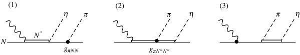
Figure 2: Dominant diagrams for $\pi$ and $\eta$ productions. The incident wavy line is either a photon or a pion. For photon induced reactions, the diagrams (1) and (2) are dominant, while for pion induced reactions, the third one (3) also contributes.

In actual computation, we take the interaction lagrangians:

$$L_{\pi NN} = g_{\pi NN}\bar{N}i\gamma_{5}\vec{\tau}\cdot\vec{\pi}N\,,\;\;\;L_{\eta NN^{*}}=g_{\eta NN^{*}}(\bar{N}\eta N^{*}+\bar{N}^{*}\eta N)\,,$$

$$L_{\pi NN^{*}} = g_{\pi NN^{*}}(\bar{N}\tau\cdot\pi N^{*}+\bar{N}^{*}\tau\cdot\pi N)$$

$$L_{\pi N^{*}N^{*}} = g_{\pi N^{*}N^{*}}(\bar{N}^{*}i\gamma_{5}\tau\cdot\pi N^{*})\,.$$ (25)

We use these interactions both for the naive and mirror cases with empirical coupling constants for $g_{\pi NN}\sim 13$, $g_{\pi NN^{*}}\sim 0.7$ and $g_{\eta NN^{*}}\sim 2$. The coupling constants $g_{\pi NN^{*}}\sim 0.7$ and $g_{\eta NN^{*}}\sim 2$ are determined from the partial decay widths, $\Gamma_{N^{*}(1535)\to\pi N}\approx\Gamma_{N^{*}(1535)\to\eta N}\sim 70$ MeV, although large uncertainties for the width have been reported. The unknown parameter is the $g_{\pi N^{*}N^{*}}$ coupling. One can estimate it by using the theoretical value of the axial charge $g_{A}^{*}$ and the Goldberger-Treiman relation for $N^{*}$. When $g_{A}^{*}=\pm 1$ for the naive and mirror assignments, we find $g_{\pi N^{*}N^{*}}=g_{A}^{*}m_{N^{*}}/{f_{\pi}}\sim\pm 17.$ Here, just for simplicity, we use the same absolute value as $g_{\pi NN}$. The coupling values used in our computations are summarized in Table 1.

Table 1: Parameters used in our calculation.

$m_{N}$	$m_{N^{*}}$	$\Gamma_{N^{*}}$	$g_{\pi NN}$	$g_{\pi NN^{*}}$	$g_{\eta NN^{*}}$	$g_{\pi N^{*}N^{*}}$
938	1535	140	13	0.7	2.0	13 (naive)
(MeV)	(MeV)	(MeV)				–13 (mirror)

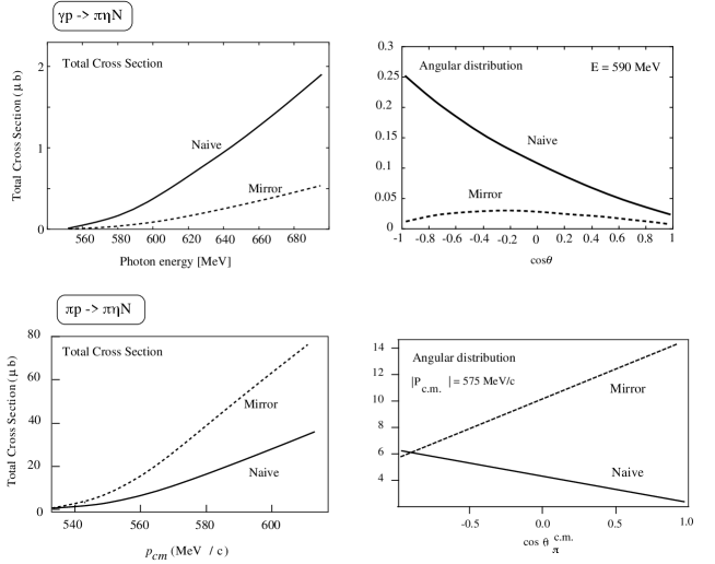
Figure 3: Various cross sections for $\pi$ and $\eta$ productions.

Several remarks follow [6]:

• We assume resonance ($N^{*}$) pole dominance. This is considered to be good particularly for the $\eta$ production at the threshold region, since $\eta$ is dominantly produced by $N^{*}$.

• There are altogether twelve resonance dominant diagrams. Due to energy denominator, the three diagrams in Fig. 2 are dominant.

• Background contributions, in which two meson (seagull) or three meson vertices appear, are suppressed due to G-parity conservation.

Hence, the processes are indeed dominated by the $N^{*}$ resonance diagrams.

We show various cross sections for the pion and photon induced processes in Fig. 3. We briefly discuss the results:

1. The total cross sections are of order of micro barn, which are well accessible by the present experiments. In the photon induced process, the diagrams (1) and (2) interfere destructively in the mirror assignment. In the pion induced case, due to the momentum dependence of the initial vertex the third term (3) becomes dominant and the mirror assignment is rather enhanced.

2. In the pion induced reaction, the angular distribution of the final state pion differs clearly depending on the sign of the $\pi NN$ and $\pi N^{*}N^{*}$ couplings.

5 Summary

In this report we have presented an algebraic argument to determine the nucleon axial charge $g_{A}$. Assuming that the nucleon belongs to a linear representation of the chiral group, the commutation relations can determine $g_{A}$. This explains the nucleon $g_{A}$ values in the non-relativistic quark model, large-$N_{c}$ and the mirror nucleons. In order to detect the mirror nucleons, we proposed an experiment of $\pi$ and $\eta$ production. Various differential cross sections were computed which can be measured at the facilities such as SPring8 and LNS, Tohoku. Determination of the axial charge is a simple but an interesting question related to chiral symmetry of the nucleon and should be studied further both in theory and experiment.

References

- [1] S. Weinberg, The Quantum Theory of Fields, Cambridge (1996), II p.203.
- [2] S. Weinberg, Phys. Rev. 177 (1969) 2604.
- [3] S. Adler, Phys, Rev. 140 (1965) B736.
- [4] W. Weisberger, Phys, Rev. 143 (1966) 1302.
- [5] D. Jido, Y. Nemoto, M. Oka and A. Hosaka, Nucl. Phys. A671 (2000) 471.
-
[6]
D. Jido, M. Oka and A. Hosaka, Prog. Theor. Phys. 106 (2001) 823;
D. Jido, M. Oka and A. Hosaka, Prog. Theor. Phys. 106 (2001) 873. - [7] S.R. Beane, Phys. Rev. D59 (1999) 031901.
- [8] A.V. Manohar, Nucl. Phys. B248 (1984) 19.
- [9] S. Weinberg, Phys. Rev. Lett. 65 (1990) 1177; 1181.
- [10] B. W. Lee, Chiral Dynamics, Gordon and Breach, New York, (1972)
- [11] C. DeTar and T. Kunihiro, Phys. Rev. D 39 (1989) 2805.