Abstract

We investigate one-loop renormalization group evolutions of extended sectors of Yukawa type couplings. It is shown that Landau Poles which usually provide necessary low energy upper bounds that saturate quickly with increasing initial value conditions, lead in some cases to the opposite behaviour: some of the low energy couplings decrease and become vanishingly small for increasingly large initial conditions! We write down the general criteria for this to happen in typical situations, highlighting a concept of repulsive quasi-fixed points, and illustrate the case both within a two-Yukawa toy model as well as in the minimal supersymmetric standard model with R-parity violation. In the latter case we consider the theoretical upper bounds on the various couplings, identifying regimes where $\lambda_{kl3},\lambda^{\prime}_{kkk},\lambda^{\prime\prime}_{3kl}$ are dynamically suppressed due to the Landau Pole. We stress the importance of considering a large number of couplings simultaneously. This leads altogether to a phenomenologically interesting seesaw effect in the magnitudes of the various R-parity violating couplings, complementing and in some cases improving the existing limits.

1 Introduction

The Infrared Quasi Fixed Point (IRQFP) structure in the Yukawa sector, [1], has played an important role in singling out the supersymmetric extension of the standard model in the small $\tan\beta$ regime, as a natural framework to accommodate a top quark mass of $\sim 175$ GeV [2], as opposed to the standard model itself or to alternatives such as the gauged Nambu–Jona-Lasinio [3] model, which predicted altogether too heavy a top quark ($\raisebox{-3.69899pt}{~{}\shortstack{$>$ \\ [-0.07cm] $\sim$}}~{}200$ GeV). The experimental (almost) negative search of Higgs particle pushes it’s mass above 114 GeV in the standard model scenario [4, 6], or above 89 GeV [5, 6] in the Minimal Supersymmetric Standard Model (MSSM), ruling out the small $\tan\beta$ IRQFP regime. This motivates naturally the study of supersymmetric scenarios where non zero bottom and $\tau$ quark Yukawa couplings are of the same order of magnitude as that of the top [7]. By the same token, one can also consider further extensions such as the next to minimal supersymmetric standard model ((M+1)SSM) [8], or the MSSM without R-parity [9], leading to an increasing number of Yukawa type couplings.

The aim of the present paper is to study the generic behaviour of the renormalization group evolutions of the Yukawa couplings in the presence of a large number of these couplings, and in particular the effect of Landau Poles on the perturbative bounds. The main result is that for increasingly large values of the initial conditions, some of the couplings can be suppressed (formally to zero!) at low energies, a behaviour which differs drastically from the usually expected one [1]. This phenomenon is related to the appearance of a rich structure of Infrared Quasi Fixed Points, some of which can have an unconventional repulsive character. In practice this means that the close numerical connection between the Landau Pole and the perturbativity bound, usually observed for the top quark Yukawa coupling for instance, does not prevail for other couplings in more general configurations.

A natural place where this new mechanism occurs is the MSSM with R-parity violation ($\not{\!\!R}_{p}$-MSSM). Here one has 45 Yukawa couplings as new free parameters to be added to those of the MSSM. In the absence of theoretically compelling reasons to put them to zero (apart from the elegant [10], yet ad hoc, R-parity!) the new parameters have to be allowed for and studied phenomenologically for their own sake. They can influence many physical processes and have already been experimentally constrained this way [29]. An important motivation for constraining R-parity violating scenarios is the bearing it can have on the nature of the supersymmetric dark matter candidate in the Universe, and indirectly on the origin of supersymmetry breaking. While conserved R-parity stabilizes the lightest supersymmetric particle (LSP) and tends to favour the lightest neutralino, rather than the gravitino, as the LSP (a natural configuration in gravity mediated supersymmetry breaking scenarios), even an extremely small violation of R-parity becomes a ”Damocles sword” over the neutralino LSP as a serious candidate for cold dark matter. Conversely, a moderate amount of R-parity violation would favour the gravitino as a potential dark matter candidate [11], and to some extent favour scenarios with low scale supersymmetry breaking.

The model-independent mechanism we elucidate in this paper can have interesting implications on the study of R-parity violation. The rest of the paper will be thus divided into two main parts –the first part, corresponding to sections 2 and 3 and appendices A and B, is devoted to a detailed discussion of the generic solutions of the one-loop renormalization group equations for an arbitrary number of Yukawa couplings, and in particular the dynamical attraction to null couplings due to the presence of Landau Poles –the second part, i.e. section 4 and appendix C, is an illustration of these features in the context of $\not{\!\!R}_{p}$-MSSM. There we study the effect of increasing the number of active couplings by considering subsets with 6, 9 and 13 non-zero couplings. We compare our results with previous theoretical bounds as well as with experimental limits. In appendix C we write explicitly the one-loop renormalization group equations governing the evolution of a large set of couplings. In section 5 we conclude and summarize our results. [The reader interested mainly in phenomenological implications on R-parity violation can go directly to section 4 which is fairly self-contained.]

2 General Formulation

2.1 Integrated Forms for the Running Yukawa Couplings

Let us consider first a general gauge theory with an arbitrary number of gauge group factors and of fermion multiplets coupled to some scalar fields. Through this paper we will always assume no flavour violating fermion-fermion-scalar Yukawa couplings. The renormalization group equations (RGE) for the gauge couplings, and [with some further simplifying assumptions about the scalar self couplings] those for the Yukawa couplings, take the following form at the one-loop level [12],

$$\frac{d}{dt}\tilde{\alpha}_{i} = -b_{i}\tilde{\alpha}^{2}_{i}$$ (1)

$$\frac{d}{dt}\tilde{Y}_{k}(t) = \tilde{Y}_{k}(t)(\sum_{i}c_{ki}\tilde{\alpha}_{i}(t)-\sum_{l}a_{kl}\tilde{Y}_{l}(t))$$ (2)

where $t\equiv Log[M_{GUT}^{2}/Q^{2}]$ denotes the scale evolution parameter, and we define

$$\tilde{Y}_{k}\equiv h_{k}^{2}/(16\pi^{2}),\;\;\tilde{\alpha}_{i}\equiv g^{2}_{i}/(16\pi^{2})$$ (3)

where $h_{k},g_{i}$ denote respectively the Yukawa and gauge couplings. The $c_{ki}$ and $a_{kl}$ are constant coefficients depending on the model.

The general solution for such a system (valid for an arbitrary number of Yukawa couplings labeled by $k$) reads [13]

$$\tilde{\alpha}_{i}(t) = \frac{\tilde{\alpha}_{i}(0)}{1+b_{i}\tilde{\alpha}_{i}(0)t}$$

$$\tilde{Y}_{k}(t) = \frac{\tilde{Y}_{k}(0)u_{k}(t)}{1+a_{kk}\tilde{Y}_{k}(0)\int_{0}^{t}u_{k}(t^{\prime})dt^{\prime}}$$ (4)

where the auxiliary functions $u_{k}$ are given by

$$u_{k}(t)=\frac{E_{k}(t)}{\raisebox{-3.69899pt}{~{}\shortstack{$\prod$ \\ [-0.07cm] ${}_{j\neq k}$}}~{}(1+a_{jj}\tilde{Y}_{j}(0)\int_{0}^{t}u_{j}(t^{\prime})dt^{\prime})^{a_{kj}/a_{jj}}}$$ (5)

and the functions $E_{k}(t)\equiv exp[\int_{0}^{t}\sum_{i}c_{ki}\tilde{\alpha}_{i}(t^{\prime})dt^{\prime}]$ read explicitly

$$E_{k}(t)=\prod\limits_{i=1}^{3}(1+b_{i}\tilde{\alpha}_{i}(0)t)^{\frac{c_{ki}}{b_{i}}}$$ (6)

In [13] we called these solutions “integrated forms” to stress the fact that they are not explicit but rather iterative. As it turned out, and will be illustrated once more in this paper, they allow, even in this form, a generic extraction of several interesting features, which could be hardly pinned down from mere numerics, in particular in relation with the infrared quasi fixed points. In many physically interesting cases such as the non supersymmetric standard model, or the MSSM or the NMSSM, the RGE’s for the Yukawa couplings take indeed the form of Eq.(2) and the above solutions are directly applicable. This is no more strictly true in the general case of $\not{\!\!R}_{p}$-MSSM, nonetheless, we will see that these solutions still prove very efficient in describing this case too.

2.2 Asymptotic behaviour and quasi fixed points

Avoiding Landau poles in the Yukawa system leads to consistency upper bounds on the values of the running Yukawa couplings at some low energy scale. These bounds can be most straightforwardly determined by looking at the asymptotic behaviour of the running couplings when some, or all, of the initial conditions are taken infinitely large. We will come back at length to the meaning of these bounds in the subsequent sections. Here we derive for further reference the complete procedure which allows a non ambiguous determination of the asymptotic behaviour, recalling and extending the point made in ref. [14]. It is useful to define

$$r_{kj}=\frac{\tilde{Y}_{k}(0)}{\tilde{Y}_{j}(0)}$$ (7)

and study the asymptotic behaviour by increasing the $\tilde{Y}_{i}(0)$’s while keeping the above scaling ratios fixed and finite ($\neq 0$). One can thus carry out the discussion in terms of the set of finite $r$’s and one single initial condition parameter $Y(0)\equiv Y^{0}$ which is allowed to become infinite. In this limit the values taken by the $\tilde{Y}_{k}(t)$ at a low energy scale $t$ are the so-called infrared effective fixed points or Infrared Quasi Fixed Points (IRQFP). From Eq.(5) one expects the $u$’s to behave like

$$u_{k}^{\infty}\equiv\frac{u_{k}^{\mathrm{QFP}}(r_{ij})}{{(Y^{0})}^{p_{k}}}$$ (8)

for asymptotically large $Y^{0}$, where we will refer to the $p_{k}$’s as “asymptotic powers”. Here $u_{k}^{\mathrm{QFP}}$ is an integrated form which is $Y^{0}$ independent but may or may not depend on the scaling parameters $r$. Now it is important to stress that Eq.(8) is quite general and does not mean that we neglect the $1$ in the denominator of Eq.(5) due to increasingly large $\tilde{Y}_{j}(0)$’s. It is indeed easy to see from Eqs.(4, 8) that the IRQFP are controlled by the various asymptotic powers in the following way,

$$\tilde{Y}_{k}^{\mathrm{QFP}}(t) = \frac{u_{k}^{\mathrm{QFP}}(t)}{a_{kk}\int_{0}^{t}u_{k}^{\mathrm{QFP}}(t^{\prime})dt^{\prime}}\;\;\;\;\;\;\;\;\mbox{if }\;p_{k}<1$$

$$\tilde{Y}_{k}^{\mathrm{QFP}}(t) = \frac{u_{k}^{\mathrm{QFP}}(t)}{1+a_{kk}\int_{0}^{t}u_{k}^{\mathrm{QFP}}(t^{\prime})dt^{\prime}}\;\;\mbox{if }\;p_{k}=1$$ (9)

$$\tilde{Y}_{k}^{\mathrm{QFP}}(t) = 0~{}~{}~{}~{}~{}~{}~{}~{}~{}~{}~{}~{}~{}~{}~{}~{}~{}~{}~{}~{}~{}\;\;\;\;\;\;\;\;\mbox{if }\;p_{k}>1$$

Only when $p_{k}<1$ is it justified to drop $1$ in the denominator. In this case the IRQFP’s take the usual form [1] as it was shown for the MSSM [18]. The two other cases in Eq.(9) occur for larger Yukawa sectors as it was found for the (M+1)SSM in [19] and for the $\not{\!\!R}_{p}$-MSSM in [14]. In particular, the very unusual configuration where some IRQFP’s vanish is worth attention. As was stressed in [14], the prior determination of the asymptotic powers is crucial. Straightforward inspection shows that they must be solutions of the following equation,

$$\vec{{\cal P}}={\cal M}\cdot(1-\vec{{\cal P}})\theta(1-\vec{{\cal P}})\vec{\delta}$$ (10)

Here $\vec{{\cal P}}$ is a column vector of all the asymptotic powers $p_{k}$; $(1-\vec{{\cal P}})\theta(1-\vec{{\cal P}})$ is a shorthand for the column vector with components $(1-p_{k})\theta(1-p_{k})\delta_{k}$ where $\theta$ is the Heaviside function, $\delta_{k}=1\;\mbox{or}\;0$ respectively for $\tilde{Y}_{k}(0)$ infinite or finite; ${\cal M}$ is defined by

$$({\cal M})_{kj}=\frac{a_{kj}}{a_{jj}}$$ (11)

Note that due to the $\theta$ function in Eq.(10) this system is linear in the $p_{k}$’s only in patches. It can thus allow simultaneously for more than one set of solutions which should correspond to alternated configurations given by Eq.(9). We will study at length the meaning of such multiple solutions in the following sections, highlighting the (new) phenomenon of repulsive IRQFP.

2.3 An example: the two-Yukawa system

It is instructive to illustrate the above as well as the forthcoming features of the paper in the simplest case of two Yukawa couplings (the “top/bottom” system):

$$\frac{d}{dt}\tilde{Y}_{1}(t) = \tilde{Y}_{1}(t)(\sum_{i}c_{1i}g^{2}_{i}(t)-a_{11}\tilde{Y}_{1}(t)-a_{12}\tilde{Y}_{2}(t))$$

$$\frac{d}{dt}\tilde{Y}_{2}(t) = \tilde{Y}_{2}(t)(\sum_{i}c_{2i}g^{2}_{i}(t)-a_{21}\tilde{Y}_{1}(t)-a_{22}\tilde{Y}_{2}(t))$$ (12)

where generically $a_{12}=a_{21}\equiv|a|,a_{11}=a_{22}\equiv|b|$ as in the MSSM (or in the Standard Model (SM)). We will stick to this configuration for simplicity although our discussion applies more generally. In this case Eq.(10) reads

$$\left(\begin{array}[]{l}p_{1}\cr p_{2}\cr\end{array}\right)=\left(\begin{array}[]{cc}0&\frac{|a|}{|b|}\cr\frac{|a|}{|b|}&0\cr\end{array}\right)\left(\begin{array}[]{l}(1-p_{1})\;\theta[1-p_{1}]\cr(1-p_{2})\;\theta[1-p_{2}]\cr\end{array}\right)$$ (13)

The critical issue here is whether $\frac{|a|}{|b|}<$ or $>1$. As can be seen from Appendix B.1, in the first case Eq.(13) has a unique solution and thus one single Infrared Quasi Fixed Point given by the first equation in (9). This case corresponds to realistic models like the SM and the MSSM (where $\frac{|a|}{|b|}=1/3$ and $1/6$ respectively). In the “toy model” case $\frac{|a|}{|b|}>1$, comparing Eqs.(13) and (B.1.1) (i.e. $\alpha=\delta=0$ and $\beta=\gamma=|a|/|b|$), one finds (see Eqs.(B.1.8, B.1.9)) that there are three different solutions to Eq.(13) corresponding to three possible IRQFP’s with the appropriate configurations in Eq.(9). Which one of these solutions is dynamically chosen by the system will be addressed in the next section. This will serve as a useful illustration, in a simple setting, of a phenomenon which actually occurs in realistic models with a large number of Yukawa couplings, such as R-parity violating models to be discussed in section 4.

3 Multiple IRQFPs and Landau Pole free domains

Let us first state the two main points we will be discussing in the next two subsections:

• The IR Quasi Fixed Points discussed in the previous section, and studied in the literature, are only isolated points on the boundary of the Landau Pole free domains (LPfd) which will be defined by Eqs.(17) (or by Eqs.(18)). Thus the “rectangle domains” given by the Quasi Fixed Points encode part but not all of the constraints on the allowed low scale values of the Yukawa couplings.

• In extended Yukawa sectors and depending on the ratios $a_{kj}/a_{jj}$ there can appear simultaneously several IR Quasi Fixed Points for the very same configuration of increasingly large initial conditions! Actually, some of these points are repulsive and others attractive, depending on the way one approaches the given configuration of initial conditions.
  

The relevance of point (II) will become manifest through the specific examples of the next sections. We just anticipate here two important and mutually related consequences: (i) the attractive IRQFP’s lead to a dynamical suppression of some of the Yukawa couplings and (ii) the perturbativity bound becomes, numerically, substantially different from the Landau Pole bound. Furthermore, it should be clear that the multiple solution scenario we will be discussing is not to be confused with the fact that one obtains different quasi fixed points for different sets of finite/infinite Yukawa initial conditions (like for the typical examples of “small $\tan\beta$” or “large $\tan\beta$” fixed point scenarios [2, 7]).

3.1 LPfd beyond the rectangular approximation

Hereafter we determine the equations defining the Landau Pole free domains (LPfd) beyond the crude “rectangular approximation”. It is convenient for the discussion to write Eq.(4) at two distinct scales $t$ and $t^{0}(<t)$ (thus $t$ corresponds to an energy scale lower than that of $t^{0}$). Eliminating $\tilde{Y}_{k}(0)$ in the ensuing equations, one obtains the general correlations between the Yukawa couplings at two arbitrary scales, expressed in a bottom-up approach where the Yukawa couplings at the high scale $t^{0}$ are cast in terms of their initial conditions at the low scale $t$ ,

$$\tilde{Y}_{k}(t^{0}) = \frac{\tilde{Y}_{k}(t)u_{k}(t^{0},t)}{1-a_{kk}\tilde{Y}_{k}(t)\int_{t^{0}}^{t}u_{k}(t^{\prime},t)dt^{\prime}}$$ (14)

where we define

$$u_{k}(t^{\prime},t) \equiv \frac{E_{k}(t^{\prime},t)}{\raisebox{-3.69899pt}{~{}\shortstack{$\prod$ \\ [-0.07cm] ${}_{j\neq k}$}}~{}(1-a_{jj}\tilde{Y}_{j}(t)\int_{t^{\prime}}^{t}u_{j}(t^{\prime\prime},t)dt^{\prime\prime})^{a_{kj}/a_{jj}}}$$ (15)

$$E_{k}(t^{\prime},t) \equiv \frac{E_{k}(t^{\prime})}{E_{k}(t)}$$ (16)

Since all the $a_{kl}$ coefficients are positive, [12], a system of non trivial constraints on the values of the $Y_{k}$’s at the scale $t$ follows,

$$\tilde{Y}_{k}(t)<\frac{1}{a_{kk}\int_{t^{0}}^{t}u_{k}(t^{\prime},t)dt^{\prime}}$$ (17)

As can be seen from Eq.(15) each of the above inequalities (for $k=1,...n$) involves all $n$ Yukawa couplings at the same scale $t$. The conjunction of all inequalities defines the allowed region in the n-dimensional parameter space of $\tilde{Y}_{k}(t)$. We should stress here that Eqs.(17) describe two different, but complementary, constraints:

- The strict inequalities preclude the $\tilde{Y}_{k}$ from becoming infinite anywhere between the low scale $t$ and the high scale corresponding to $t^{0}$. Equations (17) are thus necessary conditions guaranteeing the perturbativity of the running Yukawa’s between $t$ and $t^{0}$. But they are obviously by no means sufficient to guarantee perturbativity; when going closer and closer to the boundary of the domain defined by Eqs.(17), higher order loop contributions to the running should be included already at intermediate scales between $t$ and $t^{0}$, and a deeply non-perturbative regime is expected to set in in the vicinity of $t^{0}$. Thus the LPfd conditions have a physical meaning at the one-loop level only when considered as necessary perturbativity constraints.

- The domain defined by Eqs.(17) has yet another meaning beyond the LPfd conditions. This is simply the positivity of the $\tilde{Y}_{k}$ which are by definition the squares of the Yukawa couplings appearing in the Lagrangian. (The reader is referred to Appendix A for technical comments about the derivation of Eqs.(17).)

Without the positivity constraint, but requiring a perturbativity constraint $|\tilde{Y}_{k}(t^{0})|<\delta$, where $\delta$ is sufficiently small, one can in principle allow the domain defined by the reverse inequality in Eqs.(17). With the positivity constraint and $\tilde{Y}_{k}(t^{0})<\delta$ one obtains the improved bounds

$$\tilde{Y}_{k}(t)<\frac{\delta}{u_{k}(t^{0},t)+\delta\;a_{kk}\int_{t^{0}}^{t}u_{k}(\tau,t)d\tau}$$ (18)

which lead back to Eqs.(17) in the limit of large $\delta$. It is customary to take $\sqrt{4\pi}$ as the perturbative bound on the Yukawa couplings $h_{k}$ at the GUT scale, that is $\delta\simeq 1/(4\pi)$ when normalized as in Eq.(3). However, one can still get back approximately Eqs.(17) when $a_{kk}$ is sufficiently large. This is typically what happens for the top quark Yukawa coupling in the standard model or the MSSM: the Landau pole bound and the perturbativity bound come up numerically very close to each other even though they have theoretically different meanings. In the present paper we exhibit cases where this is no more true.

Let us illustrate the issue with the simple model of section $2.3$. In Fig.1 (a) we sketch the case $|a|/|b|<1$. Point $B$ denotes the unique IRQFP given by the first equation in (9) at a given low scale $t$ in the parameter space $(\tilde{Y}_{2}(t),\tilde{Y}_{1}(t))$. The two thick-thin dashed curves correspond each to one of the boundaries delimited by one of the two equations

$$\tilde{Y}_{1}(t) < \frac{1}{a_{11}\int_{t^{0}}^{t}u_{1}(t^{\prime},t)dt^{\prime}}$$ (19)

$$\tilde{Y}_{2}(t) < \frac{1}{a_{22}\int_{t^{0}}^{t}u_{2}(t^{\prime},t)dt^{\prime}}$$ (20)

together with (15, 16) wherein $k=1,2$ and (respectively) $j=2,1$. The conjunction of Eqs.(19, 20) gives the LPfd domain defined by the thick curves. (As they stand, the above equations are highly implicit in the variables $(\tilde{Y}_{1}(t),\tilde{Y}_{2}(t))$. Specific forms within some approximations have been given elsewhere [13].)

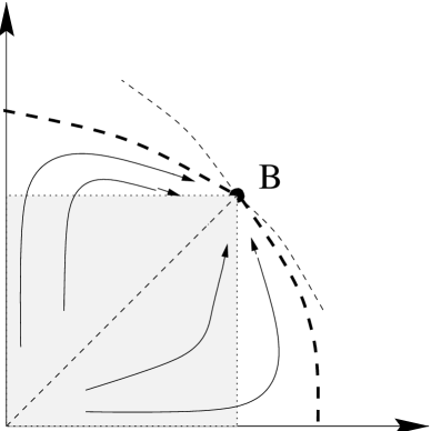
Figure 1: The IRQFP configurations for the two-Yukawa system defined in section 2.3. The thin lines represent the flow of $(\tilde{Y}_{1},\tilde{Y}_{2})$ at the low scale $t$, when the initial conditions $(\tilde{Y}_{1}(t^{0}),\tilde{Y}_{2}(t^{0}))$ are increasingly large. The different flows correspond to a different fixed ratio between these initial conditions.

A point lying on one of the thick dashed lines corresponds to a configuration where only one of the two inequalities (19, 20) is saturated, that is only one of the two initial conditions $(\tilde{Y}_{1}(t^{0}),\tilde{Y}_{2}(t^{0}))$ is infinitely large. It is point $B$, the unique intersection of the thick dashed lines which corresponds to both initial conditions becoming infinite, i.e. to the I.R. Quasi Fixed Point. This illustrates our point (I) in a specific context. The shaded rectangle would be the allowed region if one relies only on the I.R. Quasi Fixed Point. The point here is that one is still allowed to go above the IRQFP value for one of the Yukawa couplings provided that the other Yukawa coupling remains sufficiently smaller. Thus a complete analysis of the theoretically allowed domain and its comparison with the eventual experimental bounds should take into account the correlation between the Yukawa couplings. Finally we stress that the thick dashed lines are never reached, even in the limit of infinite $\tilde{Y}_{1}(t^{0}),\tilde{Y}_{2}(t^{0})$, since the only limit is point $B$. (see appendix B.2 for further discussions). In Fig. 1 (a) we show typical trajectories of the Yukawa couplings at the scale $t$. When the initial conditions at $t^{0}$ are taken large (with any fixed finite ratio $\tilde{Y}_{1}(t^{0})/\tilde{Y}_{2}(t^{0})$), all the trajectories are attracted towards $B$, even though they can still go outside of the rectangle domain. Although only qualitative and restrained to the case of two Yukawa couplings, the above features are quite generic to an arbitrary of Yukawa couplings, provided that Eq.(10) has a unique solution. This is the case for the MSSM (including all Yukawa couplings) [18] and for the (M+1)SSM [19]. The next section is devoted to the intricate configuration when Eq.(10) allows for more than one solution.

3.2 Multiple Landau Poles

We come now to point (II), first noticed in [14]. Here we give a general account, illustrate the phenomenon in the context of the simple toy model of section $2.3$, and leave to section 4 the discussion of the more complicated but physically interesting case of the MSSM with R-parity violation. As was pointed out in section $2.2$, the equation which controls the asymptotic low energy behaviour of the running Yukawas when their initial conditions are large, is in general not guaranteed to have only one solution. To start with, such a multi-solution configuration could seem mathematically inconsistent and contradicting the necessary unicity of the solutions of Eq.(2). This is actually not the case: the multi-solutions are due to the strict infinity of the initial conditions, and the unicity of the running is in fact restored for large (but finite) such conditions. However, the novelty is that the multi-solutions will all play a role here, as they will correspond either to attractive or to repulsive Quasi Fixed points. Actually, contrary to the case of a unique solution where the (finite) ratios $r_{jk}=\tilde{Y}_{j}(t^{0})/\tilde{Y}_{k}(t^{0})$ could be varied at will with no effect on the quasi fixed point, here the values of $r_{jk}$ trigger the quasi fixed point towards which the system will evolve.

Let us illustrate this phenomenon with the system defined by Eq.(12). As was shown in section 2.3 and Appendix B.1, there is potentially three different I.R. quasi fixed points, i.e. three solutions to Eq.(13). Only one of these solutions corresponds to both asymptotic powers $p_{1},p_{2}$ being smaller than one, while the two other solutions have respectively $p_{1}<1,p_{2}>1$ and $p_{1}>1,p_{2}<1$. From the discussion of section $2.2$ one then expects a quasi fixed point where both $\tilde{Y}_{1}^{\mathrm{QFP}}$ and $\tilde{Y}_{2}^{\mathrm{QFP}}$ are non vanishing, and two other quasi fixed points where one (and only one) of them vanishes, see Eq.(2.2). The question now is which of these quasi fixed points will be effectively operating at low energies? We will show that the quasi fixed points with one vanishing $\tilde{Y}^{\mathrm{QFP}}$ are the effective (attractive) ones, while the quasi fixed point with the two non-zero $\tilde{Y}^{\mathrm{QFP}}$’s is repulsive. This is illustrated in Fig.1 (b), where now the two boundary lines defined by Eqs.(19, 20) intersect in three distinct points corresponding to the three solutions, and the LPfd is delimited by the thick dashed lines. To understand the pattern of the flow depicted in the figure, let us consider a point lying close to the boundary of LPfd. Note first that, similarly to the case where $|a|/|b|<1$, this point cannot reach the LPfd boundary (when the two initial conditions $\tilde{Y}_{1}(t^{0}),\tilde{Y}_{2}(t^{0})$ become infinite) elsewhere than on points $A$, $B$ or $C$. (See appendix B.2 for a more technical discussion.) In order to guess the dynamical behaviour close to the boundary it is useful to re-write Eqs.(19, 20) in the form

$$\tilde{Y}_{k}(t)=\frac{1-\epsilon_{k}}{a_{kk}\int_{t^{0}}^{t}u_{k}(t^{\prime},t)dt^{\prime}}\;\;\;\;\;\;(k=1,2)$$ (21)

where $\epsilon_{k}>0$. This allows to write Eq.(15) in the form

$$u_{k}(t^{\prime},t)=\frac{E_{k}(t^{\prime},t)\raisebox{-3.69899pt}{~{}\shortstack{$\prod$ \\ [-0.07cm] ${}_{j\neq k}$}}~{}(\int_{t^{0}}^{t}u_{j}(\tau,t)d\tau)^{a_{kj}/a_{jj}}}{\raisebox{-3.69899pt}{~{}\shortstack{$\prod$ \\ [-0.07cm] ${}_{j\neq k}$}}~{}(\int_{t^{0}}^{t^{\prime}}u_{j}(\tau,t)d\tau+\epsilon_{j}\int_{t^{\prime}}^{t}u_{j}(\tau,t)d\tau)^{a_{kj}/a_{jj}}}.$$ (22)

The important point here is that the denominator in the above equation can potentially become very small, thus $u_{k}(t^{\prime},t)$ very large, when $\epsilon_{j}\ll 1$ and simultaneously $t^{\prime}\sim t^{0}$. But this is exactly the critical region we need to study: the behaviour of $u_{k}(t^{\prime},t)$ for $t^{\prime}\sim t^{0}$ would determine, through Eq.(21), whether $\tilde{Y}_{k}(t)$ goes to zero when $\epsilon_{k}\to 0$, that is whether the system is attracted towards points $A$ or $C$, rather than $B$, when approaching the boundary of LPfd. Because in Eq.(22) the $u_{k}$’s are defined iteratively in terms of one another , we are lead to considerations similar to those of section 2.2 where now in Eq.(8) $Y^{0}$ is replaced by $\epsilon_{k}$. A more sophisticated treatment leading to equations similar to Eq.(10) is required though and is deferred to appendix B.2. The bottom line is as follows: if we consider the hierarchical regime such as $\epsilon_{2}\ll\epsilon_{1}\raisebox{-3.69899pt}{~{}\shortstack{$<$ \\ [-0.07cm] $\sim$}}~{}1$ which corresponds to a point lying very close to the LPfd boundary between points $B$ and $C$, then the solutions to Eqs.(B.2.7, B.2.8) imply unambiguously that $\int_{t^{0}}^{t}u_{1}(t^{\prime},t)dt^{\prime}\sim\epsilon_{2}^{-|\Delta|}$, where $|\Delta|$ is a positive number uniquely determined by these equations. Combined with Eq.(21), this behaviour means that the system is dynamically attracted to point $C$. Similarly, if we consider $\epsilon_{1}\ll\epsilon_{2}\raisebox{-3.69899pt}{~{}\shortstack{$<$ \\ [-0.07cm] $\sim$}}~{}1$, then the system will be attracted to point $A$. This leads altogether to the flow pattern of Fig.1 (b). Actually, it is still possible to land on point $B$, but only at the price of a delicate fine-tuning corresponding to the trajectory satisfying $\tilde{Y}_{1}(t)=\tilde{Y}_{2}(t)$, especially when $|a|/|b|$ is much larger than one. In Fig.2 we show a purely numerical analysis staring directly from the differential equations (12) with $a=1(\mbox{resp.}\;6)$ and $b=6(\mbox{resp.}\;1)$. The results confirm nicely the above theoretical arguments. Fig.2 (a) illustrates the insensitivity to the values of $r_{12}\equiv\tilde{Y}^{0}_{1}/\tilde{Y}^{0}_{2}$ near the IRQFP. In contrast, one notes the high sensitivity to this ratio in the configuration of Fig. 2 (b), due to the presence of multiple Landau Poles. In particular, the attraction to point $B$ in Fig. 2 (b) occurs at the price of fine-tuning $r_{12}$ to $1$ to less than $0.1$ per mil, otherwise the system is strongly attracted to points $A$ or $C$ depending on whether $r_{12}$ is greater or smaller than one.

Figure 2: A numerical illustration of the behaviour of the toy model Eqs.(12) with $|a|=1,|b|=6$ in a) and $|a|=6,|b|=1$ in b). The running $\tilde{Y}_{1}(t),\tilde{Y}_{2}(t)$ are evaluated at $t=66$. The smallest initial condition $\tilde{Y}^{0}_{i}$ is varied from 0 to 1000. Near the IRQFP’s, the insensitivity to $r_{12}$ in a) and the high sensitivity to $r_{12}$ in b) are manifest.

To summarize this section on the two-Yukawa system, we have shown in general that when $r_{12}$ is neither infinite nor zero, the LPfd boundary closes only on a set of isolated points, point $B$ in the case of Fig.1 (a) and points $A$, $B$, $C$ in the case of Fig.1 (b). Most of the LPfd boundary, the thick dashed lines, can be closely approached but is actually never reached, the system being eventually driven to one of the above points. In Fig.1 (a), only when $r_{12}$ is infinite or zero (i.e. one of the initial conditions remains finite) does one retrieve the effective fixed point à la Hill, in which case point $B$ becomes located on one of the two axes. Of particular importance is the case of Fig.1 (b). It shows how the existence of multiple IRQFP’s fits nicely with the phenomenon of dynamical attraction to or repulsion from such points, leading to the unusual suppression of some couplings. This is quite a general mechanism which occurs beyond the two-Yukawa system as will be illustrated in the next section. Finally we would like to insist on the fact that although a perturbative analysis is trustful only far from these IRQFP’s, the latter remain nevertheless very useful in understanding the generic behaviour of the low energy perturbative couplings, as they play the role of a far away beacon for such a behaviour.

4 $\not{\!\!R}_{p}$-MSSM

In this section we concentrate on a phenomenological application in the context of the MSSM with R-parity violation. The unusual behaviour near Landau Poles was indeed first noticed in this context [14].

Let us first recall the form of the superpotential in $\not{\!\!R}_{p}$-MSSM:

$$W_{\not{R}_{p}}=W+W_{\not{L}}+W_{\not{B}}$$ (23)

where $W$ is the R-parity conserving part

$$W=(h_{E})_{ij}L_{L}^{i}.H_{1}\bar{E}_{R}^{j}+(h_{D})_{ij}Q_{L}^{i}.H_{1}\bar{D}_{R}^{j}+(h_{U})_{ij}Q_{L}^{i}.H_{2}\bar{U}_{R}^{j}+\mu H_{1}.H_{2}$$ (24)

$W_{\not{L}}$ induces lepton number violation,

$$W_{\not{L}}=\frac{1}{2}\lambda_{ijk}L_{L}^{i}.L_{L}^{j}\bar{E}_{R}^{k}+\lambda^{\prime}_{ijk}L_{L}^{i}.Q_{L}^{j}\bar{D}_{R}^{k}+\kappa_{i}L_{L}^{i}.H_{2}$$ (25)

and $W_{\not{B}}$ induces baryon number violation,

$$W_{\not{B}}=\frac{1}{2}\lambda^{\prime\prime}_{ijk}\bar{U}_{R}^{i}\bar{D}_{R}^{j}\bar{D}_{R}^{k}.$$ (26)

The superfields $L_{L},Q_{L},\bar{E}_{R},\bar{D}_{R},\bar{U}_{R}$ denote lepton and quark $SU(2)$ doublets and anti-singlets, $H_{1},H_{2}$ the two Higgs doublets. Summation on $SU(3)$ color indices is implicit and the dots ($A\cdot B\equiv\epsilon_{ab}A_{a}B_{b}$) define SU(2) invariants The $i,j,k=1,2,3$ are generation indices, and summation is understood for repeated indices.

We will rely hereafter on [21] ([22]) to write down the RGE’s at the one-loop level. The relation between the above $\lambda$’s and their matrices ${\bf\Lambda}$ is as follows:

$$\lambda_{ijk}\equiv({\bf\Lambda}_{E^{k}})_{ij},\lambda^{\prime}_{ijk}\equiv({\bf\Lambda}_{D^{k}})_{ij},\lambda^{\prime\prime}_{ijk}\equiv({\bf\Lambda}_{U^{i}})_{jk}.$$

(Note that the notation is consistent with that of [21], but differs for instance from [16] only in $\lambda^{\prime\prime}$.) The matrices ${\bf\Lambda}_{E^{k}}$ and ${\bf\Lambda}_{U^{k}}$ being anti-symmetric, lead to a total of 18 couplings, while ${\bf\Lambda}_{D^{k}}$ give 27 extra couplings. We will not consider hereafter the bi-linear couplings $\kappa^{i}$ and $\mu$ as their renormalization group evolution does not affect that of the Yukawa couplings we are interested in, [21], [22].

The issue of theoretical bounds on RPV couplings has been addressed in various papers [15, 16, 17, 27, 28], either from the point of view of exact infrared fixed points, when they exist, or from that of perturbativity and/or effective fixed points related to Landau Pole considerations. However, often a rather reduced number of couplings has been considered which may not exhibit the behaviour we described in the previous sections. Typically, the larger the number of couplings, and accordingly the dimension of ${\cal M}$ in Eq.(10), the more likely it is to find asymptotic powers significantly greater than $1$ as solutions to this equation, leading to a dynamical suppression of some Yukawa couplings due to the Landau pole.

As was first shown in [14], the system of 6 couplings $h_{t},h_{b},h_{\tau},\lambda_{233},\lambda^{\prime}_{333},\lambda^{\prime\prime}_{323}$ does exhibit such a behaviour where $\lambda^{\prime}_{333}$ decreases while the other couplings increase towards their perturbativity bound.

On the other hand, there are also numerical studies of the simultaneous renormalization group evolution of all 45 Yukawa couplings, putting the accent on the correlation between experimental bounds at low energy and initial values at the grand unified scale [23].

Here we take up a fairly complementary approach. We consider various sectors with 13 couplings chosen in such a way as to encompass previous studies as subclasses and in the same time to be realistic enough for phenomenology. These sectors allow also a direct application of the analytic criteria developed in the previous sections and a clear numerical illustration of these criteria.

RPV₁₃ sectors: Each of these sectors has 13 couplings and is defined as follows. For fixed $k$ and fixed $l(\neq k)$ we consider the RGE’s associated to the system

$${\bf RPV{}_{13}}\equiv(h_{t},h_{b},h_{\tau},\lambda_{klq},\lambda^{\prime}_{kkk},\lambda^{\prime}_{kkl},\lambda^{\prime}_{klk},\lambda^{\prime}_{lkk},\lambda^{\prime\prime}_{qkl}),\;\;\mbox{where}\;\;q=1,2,3$$ (27)

Thus one has for each case three $\lambda$’s, three $(\lambda^{\prime\prime})$’s and four $(\lambda^{\prime})$’s. The RGE’s in the RPV₁₃ sectors are explicitly written in appendix C. One can see that they have strictly the form of Eq.(2) when $k\neq 3$. For $k=3$, Eqs.(C.2, C.3, C.6, C.10) deviate by one extra term from this form, but as we will see throughout the numerical analysis, the behaviour is still dictated by our general criteria. Actually the specific choice of the set (27) is motivated by the opportunity to remain as close as possible to the form of Eqs.(2). We stress here that this is not necessarily the only possibility, but we stick to it as a working hypotheses which allows for general enough, yet analytically tractable, illustrations.

4.1 Asymptotic powers

To start with, it is instructive to follow the variation of the asymptotic powers when the number of active RPV couplings is increased.

RPV₆: Consider the set of non zero couplings $(h_{t},h_{b},h_{\tau},\lambda_{233},\lambda^{\prime}_{333},\lambda^{\prime\prime}_{323})$. This is a subset of Eq.(27) with $k=q=3$ and $l=2$. Here the order of the antisymmetric indices is irrelevant, since the evolution equations in the RPV₆ subset are blind to the sign of the couplings, as can been seen from Appendix C. In this case Eq.(10) reads

$$\left(\begin{array}[]{l}p_{t}\cr p_{b}\cr p_{\tau}\cr p_{233}\cr p^{\prime}_{333}\cr p^{\prime\prime}_{323}\cr\end{array}\right)=\left(\begin{array}[]{llllll}0&\frac{1}{6}&0&0&\frac{1}{6}&\frac{1}{3}\cr\frac{1}{6}&0&\frac{1}{4}&0&1&\frac{1}{3}\cr 0&\frac{1}{2}&0&1&\frac{1}{2}&0\cr 0&0&1&0&\frac{1}{2}&0\cr\frac{1}{6}&1&\frac{1}{4}&\frac{1}{4}&0&\frac{1}{3}\cr\frac{1}{3}&\frac{1}{3}&0&0&\frac{1}{3}&0\end{array}\right)\left(\begin{array}[]{l}(1-p_{t})\;\theta[1-p_{t}]\;\delta_{t}\cr(1-p_{b})\;\theta[1-p_{b}]\;\delta_{b}\cr(1-p_{\tau})\;\theta[1-p_{\tau}]\;\delta_{\tau}\cr(1-p_{233})\;\theta[1-p_{233}]\;\delta_{0}\cr(1-p^{\prime}_{333})\;\theta[1-p^{\prime}_{333}]\;\delta_{1}\cr(1-p^{\prime\prime}_{323})\;\theta[1-p^{\prime\prime}_{323}]\;\delta_{2}\cr\end{array}\right)$$ (28)

Solving this equation in the regime where all $\delta^{\prime}s=1$, one finds that $p_{t},p_{b},p_{233},p^{\prime\prime}_{323}<1$ while $p^{\prime}_{333}=\frac{5}{4}$ and $p_{\tau}=\frac{23}{17}$ meaning that the running $\lambda^{\prime}_{333}$ and $h_{\tau}$ at any sufficiently low energy scale will decrease to zero with increasing initial values at the GUT scale. However, since $p^{\prime}_{333},p_{\tau}$ are close to $1$ this decrease is relatively slow, [14]. Actually Eq.(28) has yet another solution with all asymptotic powers smaller than $1$; but this solution turns out to be repulsive in the sense of sections 3.2 and B.2. In Fig. 3 we illustrate the evolution of the RPV₆ system, solving purely numerically [24] the corresponding RGE’s as given in appendix C.

Figure 3: The running couplings of the RPV₆ system evaluated at $t=66\simeq Log[M_{GUT}^{2}/M_{Z}^{2}]$, as a function of their common initial condition $\lambda^{0}$. $\lambda^{\prime}_{333}$ and $\lambda_{\tau}$ decrease very slowly even for $\lambda^{0}\gg\lambda^{0}_{pert}$.

The decrease of $\lambda^{\prime}_{333}$ and $h_{\tau}$ with an increasing common value of the initial condition $\lambda^{0}$ nicely confirms the above expectations. However, since the corresponding asymptotic powers are close to $1$, the dynamical suppression is too slow to be sizeable before the perturbativity bound at the GUT scale, defined for instance as $\lambda^{0}_{pert}=\sqrt{4\pi}\simeq 3.54$, is reached.

RPV₉: Adding $\lambda^{\prime}_{233},\lambda^{\prime}_{323},\lambda^{\prime}_{332}$ to the previous set of couplings and solving the corresponding Eq.(10) with the help of algebraic packages [25] (the relevant $9\times 9$ matrix ${\cal M}_{9}$ can be straightforwardly extracted from ${\cal M}_{13}$ in Eq.(29) below) one now finds a larger value for $p^{\prime}_{333}(\simeq 1.67)$. The decrease in $\lambda^{\prime}_{333}$ becomes strong enough to build in significantly before the perturbativity bound at the GUT scale is reached. Note that there are, here too, more than one set of solutions, actually three, but all of them have the above value for $p^{\prime}_{333}$. The dynamically chosen solution has also $p_{b}\simeq 1.16$ and $p_{323}\simeq 1.3$. Again, we have illustrated in Figs.4 (a), (b) the numerical results obtained directly from the RGE’s of the RPV₉ system and which confirm the above asymptotic power behaviour. Comparing Fig.3 with Fig.4 (a), we see how the activation of a bigger number of RPV couplings strengthens the bounds on some of these couplings, in particular the drastic drop of $\lambda^{\prime}_{333}$ in the RPV₉ as compared to the RPV₆ case, or to the case of smaller number of active couplings like in [16]. The price to pay is a looser bound on the extra couplings as shown in Fig.4 (b).

Figure 4: The running couplings of the RPV₉ system evaluated at $t=66\simeq Log[M_{GUT}^{2}/M_{Z}^{2}]$, as a function of their common initial condition $\lambda^{0}$.

RPV₁₃: Addition of new couplings does not necessarily make the dynamical suppression of one single coupling more pronounced, but can rather propagate this suppression to other couplings. This is indeed the case when all 13 couplings as defined in Eq.(27) with $k=3$, are simultaneously activated. The corresponding matrix of Eq.(11) is easily read from appendix C:

$${\cal M}_{13}=\left(\begin{array}[]{lllllllllllll}0&\frac{1}{6}&0&0&0&0&\frac{1}{6}&\frac{1}{6}&0&\frac{1}{6}&0&0&\frac{1}{3}\cr\frac{1}{6}&0&\frac{1}{4}&0&0&0&1&\frac{1}{6}&\frac{1}{3}&1&\frac{1}{3}&\frac{1}{3}&\frac{1}{3}\cr 0&\frac{1}{2}&0&\frac{1}{4}&\frac{1}{4}&1&\frac{1}{2}&\frac{1}{2}&\frac{1}{2}&0&0&0&0\cr 0&0&\frac{1}{4}&0&1&1&\frac{1}{2}&\frac{1}{2}&\frac{1}{2}&\frac{1}{2}&0&0&0\cr 0&0&\frac{1}{4}&1&0&1&\frac{1}{2}&\frac{1}{2}&\frac{1}{2}&\frac{1}{2}&0&0&0\cr 0&0&1&1&1&0&\frac{1}{2}&\frac{1}{2}&\frac{1}{2}&\frac{1}{2}&0&0&0\cr\frac{1}{6}&1&\frac{1}{4}&\frac{1}{4}&\frac{1}{4}&\frac{1}{4}&0&1&1&1&\frac{1}{3}&\frac{1}{3}&\frac{1}{3}\cr\frac{1}{6}&\frac{1}{6}&\frac{1}{4}&\frac{1}{4}&\frac{1}{4}&\frac{1}{4}&1&0&\frac{1}{2}&\frac{1}{6}&\frac{1}{3}&\frac{1}{3}&\frac{1}{3}\cr 0&\frac{1}{3}&\frac{1}{4}&\frac{1}{4}&\frac{1}{4}&\frac{1}{4}&1&\frac{1}{2}&0&\frac{1}{3}&\frac{1}{3}&\frac{1}{3}&\frac{1}{3}\cr\frac{1}{6}&1&0&\frac{1}{4}&\frac{1}{4}&\frac{1}{4}&1&\frac{1}{6}&\frac{1}{3}&0&\frac{1}{3}&\frac{1}{3}&\frac{1}{3}\cr 0&\frac{1}{3}&0&0&0&0&\frac{1}{3}&\frac{1}{3}&\frac{1}{3}&\frac{1}{3}&0&1&1\cr 0&\frac{1}{3}&0&0&0&0&\frac{1}{3}&\frac{1}{3}&\frac{1}{3}&\frac{1}{3}&1&0&1\cr\frac{1}{3}&\frac{1}{3}&0&0&0&0&\frac{1}{3}&\frac{1}{3}&\frac{1}{3}&\frac{1}{3}&1&1&0\end{array}\right)$$ (29)

In this case (again with all $\delta^{\prime}s=1$), one finds, with the help of algebraic packages [25], 14 different solutions to Eq.(10). All these solutions have in common $p^{\prime}_{333}\raisebox{-3.69899pt}{~{}\shortstack{$>$ \\ [-0.07cm] $\sim$}}~{}1.43$ and $p^{\prime\prime}_{332}\sim 1.3$. In particular, the dynamically chosen solution exhibits new features: $p^{\prime}_{333}$ has decreased slightly to $\simeq 1.46$ as compared to the RPV₉ case, but now $p_{323}$ and $p^{\prime\prime}_{332}$ are $\sim 1.3$ and $p^{\prime}_{233}\sim 1.06$; the asymptotic powers of all other couplings remain smaller than one. This means that the three couplings $\lambda_{323},\lambda^{\prime}_{333},\lambda^{\prime\prime}_{332}$ are dynamically driven to zero by the Landau Pole, and in any case decrease significantly, well before the perturbativity bound is reached, as confirmed by the numerical analysis shown in Fig.5 (a), (b); $\lambda^{\prime}_{233}$ is also dynamically driven to zero but decreases very slowly since its asymptotic power is very close to $1$.

[Note that all the above conclusions hold as well for $l=1$, i.e. for $\lambda_{133},\lambda^{\prime}_{333},\lambda^{\prime\prime}_{313}$, etc… since ${\cal M}_{13}$ is $l$ independent. ]

Figure 5: The running couplings of the RPV₁₃ system evaluated at $t=66\simeq Log[M_{GUT}^{2}/M_{Z}^{2}]$, as a function of their common initial condition $\lambda^{0}$.

4.2 Theoretical bounds on the RPV couplings

As can be seen from Figs.3,4,5, the couplings which increase with $\lambda^{0}$ actually saturate and become quickly weakly sensitive to $\lambda^{0}$. This is why the perturbativity bound for the low energy couplings is sometimes associated to the Landau Pole. This is indeed typically the case for the top, bottom and $\tau$ Yukawa couplings in the R-parity conserving MSSM. However, the fact that the perturbativity bound and the Landau Pole are in general disconnected is nicely illustrated by those couplings which decrease with increasing $\lambda^{0}$ and are sensitive to its values. For instance, in RPV₉ and RPV₁₃, $\lambda^{\prime}_{333}$ drops by more than a factor of 2 of its maximal value, when $\lambda^{0}$ reaches $\sqrt{4\pi}$. Moreover, the perturbativity bound on $\lambda^{\prime}_{333}$ (taken here at $M_{susy}=1$ TeV) drops drastically, from $0.52$ in RPV₆ to $0.12-0.13$ in RPV₉ and RPV₁₃, as can be seen from the figures. These bounds are way below the ones usually quoted.

In order to have a realistic comparison, also with the existing experimental bounds, one has to require consistency with the experimental top, bottom and $\tau$ fermion masses. This translates into the following constraints

$$h_{t}(m_{t})=\frac{m_{t}\;(2\sqrt{2}G_{F})^{\frac{1}{2}}}{\sin\beta},\;\;\;h_{b,\tau}(m_{t})=\frac{m_{b,\tau}(m_{t})\;(2\sqrt{2}G_{F})^{\frac{1}{2}}}{\cos\beta}$$ (30)

where $G_{F}$ is the Fermi constant $(=1.166\times 10^{-5}$ GeV), $m_{t}$ is the running top quark mass at its fixed point value $m_{t}(m_{t})=m_{t}$, and $m_{b,\tau}(m_{t})$ are the running bottom and $\tau$ masses at this value. We take $m_{t}=165$ GeV, $m_{b}(m_{t})=2.76$ GeV and $m_{\tau}(m_{t})=1.78$ GeV. Furthermore, we will also require unification of the three gauge couplings at $M_{GUT}=2\times 10^{16}$ GeV. Keeping in mind that we are not seeking here a very precise gauge unification analysis since the running is performed only at one-loop level, we tolerate a deviation of the value of $\alpha_{s}(M_{Z})$ from the one determined by LEP precision measurements, as well as a susy scale $\sim M_{Z}$ in order to achieve one-loop gauge unification with the proper normalization ($(5/3)\times g_{1}^{2}(GUT)=g_{2}^{2}(GUT)=g_{3}^{2}(GUT)$). It should be clear, however, that a more sophisticated treatment of this sector would not change the main features related to the dynamical behaviour of the RPV couplings.

We take the following values for the fine structure constant $\alpha_{em}$, $\alpha_{s}$ and $\sin^{2}\theta_{W}$ at the $M_{Z}$ scale

$$\alpha_{em}(M_{Z})=1/127.938,\;\;\alpha_{s}(M_{Z})=0.1169,\;\;\sin^{2}\theta_{W}(M_{Z})=0.23117$$ (31)

(of which $\alpha_{s}$ deviates by $0.2\%$ from the experimental value [26].)

In order to study the effect of Landau Poles, the numerical algorithm will have to meet the requirement of maximizing the initial Yukawa conditions at the GUT scale, while keeping consistency with Eq.(30). This is not straightforward due to the large number of couplings. As we stressed in previous sections, Landau Pole constraints (or for that matter, perturbativity constraints) delimit hypervolume domains in the space of couplings. The numerical values obtained correspond only to specific directions in this space, depending on which set of couplings is made large at the GUT scale. It is important to determine the directions which allow the largest possible values for all the couplings.

In practice, we proceed as follows: for a given $\tan\beta$, and assuming a common susy scale much higher than the top mass, we first run the (non supersymmetric) standard model top, bottom and $\tau$ Yukawa couplings from their values at $m_{t}$ scale as given by Eq.(30) up to $M_{susy}$ scale. From there we run these couplings up to the GUT scale within the (R-parity conserving) MSSM. There we switch on all the RPV couplings of a given RPV_n sector, giving them in a first step a common and large value at the GUT scale $\lambda^{init}_{GUT}$, run the $n$ Yukawa couplings of the RPV_n sector down to $M_{susy}$, re-adjust $h_{t},h_{b},h_{\tau}$ to their previously determined values consistent with Eq.(30) and run the RPV_n sector back to $M_{GUT}$. If at least one coupling is greater than the perturbative bound (taken to be $\sqrt{4\pi}$) then the procedure is iterated starting from a smaller $\lambda^{init}_{GUT}$, in the opposite case $\lambda^{init}_{GUT}$ is increased and the procedure iterated until the largest coupling at the GUT scale reaches the limit $\sqrt{4\pi}$ (within 1 per mil). However, even then, there is no guarantee that the other couplings have been optimally maximized, since the procedure starts with a unified value of the RPV’s at the GUT scale. This is why a further step is taken after numerical convergence: start with the obtained solution at $M_{susy}$, scale up some of the RPV’s and down some others, by the same factor, then run up to $M_{GUT}$ and check for perturbativity. Again the procedure stops after convergence to the optimal scaling factor. The numbers thus obtained at the susy scale correspond to theoretical perturbativity bounds on the various couplings. It is important to note here the existence of a seesaw effect between some specific sub-classes of RPV couplings. The above inverted scaling works when these sub-classes are properly chosen. For instance, in RPV₁₃, the dynamically suppressed couplings $\lambda_{3l3},\lambda^{\prime}_{333},\lambda^{\prime\prime}_{33l}$ (see Fig.5) can be increased at the price of lowering the remaining ones.

Figure 6: The running couplings of the RPV₁₃ system evaluated at the susy scale $M_{SUSY}=1$TeV ($t\simeq 61.25$), as a function of $\tan\beta$, subject to the constraints $m_{t}(m_{t})=165$ GeV, $m_{b}(m_{t})=2.76$ GeV, $m_{\tau}(m_{t})=1.78$ GeV and unification of gauge couplings at $M_{GUT}=2\times 10^{16}$ GeV. Figures a) and b) ( resp. c) and d) ) are two different configurations where the perturbativity bound $\sqrt{4\pi}$ is reached by one of the couplings at the GUT scale.

In Fig.6 we illustrate these effects as a function of $\tan\beta$ in the case RPV₁₃. The difference between Figs. (a), (c) on one hand and Figs. (b), (d) on the other, shows clearly that it is possible to increase, for instance, the magnitudes of $\lambda_{3l3},\lambda^{\prime}_{333}$ for any value of $\tan\beta$, but various other $\lambda^{\prime},\lambda^{\prime\prime}$ couplings should be decreased accordingly, in order to remain consistent with the constraints described above. This seesaw effect is actually far more general than what is illustrated in the figure and occurs for the sets of $\lambda$’s, $(\lambda^{\prime})$’s and $(\lambda^{\prime\prime})$’s either separately or in some combinations of them; it is triggered by the fact that not all couplings can be simultaneously increased (or decreased) without conflicting with the dynamical suppression mechanism explained before. Also the magnitude of the effect tends to increase with decreasing $\tan\beta$. For instance, if $\tan\beta\raisebox{-3.69899pt}{~{}\shortstack{$<$ \\ [-0.07cm] $\sim$}}~{}10$ one can raise $\lambda^{\prime\prime}_{33l}$ up to $\sim 0.97$ at the price of reducing all the remaining RPV₁₃ couplings down to $\raisebox{-3.69899pt}{~{}\shortstack{$<$ \\ [-0.07cm] $\sim$}}~{}0.17$ for the $\lambda$’s and $\lambda^{\prime}_{333}$, and down to $\raisebox{-3.69899pt}{~{}\shortstack{$<$ \\ [-0.07cm] $\sim$}}~{}0.3$ for the other $\lambda^{\prime}$, $\lambda^{\prime\prime}$. For higher $\tan\beta$ values these bounds drop further down: when $\tan\beta\sim 60$, $\lambda^{\prime\prime}_{33l}\sim 0.84$, while $\lambda^{\prime\prime}_{13l},\lambda^{\prime\prime}_{23l}\sim 0.15$, $\lambda_{3l3}\sim 3\times 10^{-2}$, $\lambda_{3l1},\lambda_{3l2},\lambda^{\prime}_{l33}\sim 7.7\times 10^{-2}$, $\lambda^{\prime}_{333}\sim 6.8\times 10^{-2}$ and $\lambda^{\prime}_{3l3},\lambda^{\prime}_{33l}\sim 0.12$. (Similar effects obtain if one chooses to raise the bound for $\lambda^{\prime}_{333}$; we will come back to that in the next section when comparing with the present experimental limits.) We thus see that Fig.6 is with many respects a conservative illustration of the perturbativity bounds one can obtain.

Note that although the top/bottom/$\tau$ Yukawa couplings are uniquely determined in terms of $\tan\beta$ through the fermion masses at the relevant low scale, Eq.(30), their running values above the susy scale are still affected by the RPV system. In particular, the GUT scale values of $h_{b},h_{\tau}$ remain small for $\tan\beta\raisebox{-3.69899pt}{~{}\shortstack{$<$ \\ [-0.07cm] $\sim$}}~{}40$ where $\lambda^{\prime}_{333}$ or $\lambda_{3l3}$ are those which saturate the perturbativity bound, while for $40\raisebox{-3.69899pt}{~{}\shortstack{$<$ \\ [-0.07cm] $\sim$}}~{}\tan\beta\raisebox{-3.69899pt}{~{}\shortstack{$<$ \\ [-0.07cm] $\sim$}}~{}60$, $h_{b}$ then $h_{\tau}$ take over gradually in saturating this bound.

The main lesson to draw from this section is the importance of including as many couplings as possible in order to achieve a complete study of the perturbativity bounds. The results obtained here for the RPV₁₃ system yield much stronger perturbativity bounds on $\lambda^{\prime}$ and $\lambda^{\prime\prime}$ than previously found [27, 28]. (see for instance the bracketed numbers displayed in the compilation Table 1 of ref. [23]). The latter vary in the range $1.04-1.23$ while ours can hardly reach $1$ for some couplings while the others are anyway bound to be much smaller. The fact that stronger bounds ensue from activating a larger number of couplings was already exemplified in [27, 28], since there the upper bound $1.23$ was on $\sqrt{\sum_{l}{\lambda^{\prime\prime}_{33l}}^{2}}$ rather than on individual couplings. A similar effect is actually observed in our numerical study, nonetheless it should be considered as a “phase space” effect which is complementary, but distinct, from the dynamical suppression effect we have studied throughout the previous sections.

4.3 Comparison with the experimental bounds

Bounds on RPV couplings from experimental data have been extensively studied in the literature, ranging from nuclear and atomic physics to astrophysics, as well as high energy accelerator physics, (see [30], [29] and references therein and there out). Since we are considering several $\lambda,\lambda^{\prime},\lambda^{\prime\prime}$ in a time, a systematic comparison with the above bounds is certainly out of the scope of the present paper. Indeed, these bounds are usually established keeping a minimal set of couplings in a time [30, 31, 32], in particular for the very strong ones on the products $\lambda\times\lambda^{\prime\prime}$ from proton stability [33] or on $\lambda\times\lambda$, $\lambda^{\prime}\times\lambda^{\prime}$ from neutrino masses [34]. We shall thus limit the discussion here to some representative examples. We stress here that the various experimental limits on individual couplings at the weak scale (see for instance Table 1 of ref. [23]), if one assumes a common susy mass of $\tilde{m}=1$ TeV, can be in general easily overwhelmed by the theoretical perturbativity bounds we have found in the RPV₁₃ system. Comparing for instance to the configuration of Fig.6, the experimental limits on $\lambda_{321},\lambda_{322},\lambda_{323}\sim 0.7$ are about a factor of two weaker than our perturbativity bound, except for $\lambda_{323}$ at low $\tan\beta$ in the configuration of Fig.6 (b) where they become comparable. However, in the latter configuration the perturbativity bounds on $\lambda^{\prime}_{233},\lambda^{\prime}_{323},\lambda^{\prime}_{332}\raisebox{-3.69899pt}{~{}\shortstack{$<$ \\ [-0.07cm] $\sim$}}~{}0.3$ are stronger than the experimental limits. Of course there are configurations where the experimental limits become, at least for some couplings, stronger than the perturbativity bounds. This is true in particular if one takes into account recent limits from proton stability [33] and neutrino physics [34]. If we pick up for instance the configuration where $\lambda^{\prime\prime}_{33l}\sim 0.84$ (see previous sub-section) then the perturbativity bound on the products $\lambda_{3l3}\lambda^{\prime\prime}_{33l},\lambda_{3l1}\lambda^{\prime\prime}_{33l},\lambda_{3l2}\lambda^{\prime\prime}_{33l}\sim 2.5\times 10^{-2}-6.5\times 10^{-2}$ is overwhelmed by the proton stability limits by several orders of magnitude [33]. For the same configuration one has the perturbativity bounds $\lambda^{\prime}_{333}\sim 6.8\;(3.6)\;\times 10^{-2}$ and $\lambda_{3l3}\sim 3\;(1.9)\;\times 10^{-2}$, where the numbers in brackets correspond to a lower susy scale $m_{susy}=100$ GeV. These bounds are clearly stronger than the experimental limits obtained from specific $\tau$ lepton and $Z$ boson branching ratios measurements, but they remain two orders of magnitude weaker than those from neutrino physics [34]. However they are still meaningful in various respects: (i) they correspond to a situation where many couplings are active simultaneously, while the bounds from neutrino physics and proton stability are obtained within reduced sets or simplifying working assumptions [34, 33], barring possible cancellations effects which could in principle weaken substantially the latter bounds. (ii) They are of the same order both for $m_{susy}=100$ GeV or $1$ TeV, while experimental bounds from neutrino physics are derived assuming $m_{susy}=100$ GeV. (iii) In both proton stability and neutrino physics it is not clear how low energy QCD effects between virtual quarks and squarks at $\lambda^{\prime\prime}$ and $\lambda^{\prime}$ vertices would affect the extraction of the experimental bounds. The running RPV’s are in principle free from such uncertainties insofar as their low energy values are frozen at the susy scale.

In the case where $m_{susy}\simeq 100$ GeV, most of the $2\sigma$ limits on the RPV’s are a factor of ten stronger than for $m_{susy}\simeq 1$ TeV. The perturbativity bounds are then overrun for small and moderate $\tan\beta$ values, in particular for the $\lambda$’s of RPV₁₃, but not necessarily for the ($\lambda^{\prime}$)’s and ($\lambda^{\prime\prime}$)’s. For instance, $\tan\beta\simeq 10$ leads, for a configuration where $\lambda^{\prime\prime}_{13l}$ is maximized ($\simeq 1.09$), to $\lambda^{\prime\prime}_{23l}\simeq 0.34,\lambda^{\prime\prime}_{33l}\simeq 0.28$, $\lambda^{\prime}_{333}\simeq 0.18$, $\lambda^{\prime}_{33l},\lambda^{\prime}_{3l3},\lambda^{\prime}_{l33}\simeq 0.3$, while $\lambda_{3lq}\simeq 0.18$. For $\tan\beta$ as large as $60$, $\lambda^{\prime\prime}_{13l}$ maximizes to $0.62$ and $\lambda^{\prime\prime}_{23l}\simeq 0.15,\lambda^{\prime\prime}_{33l}\simeq 0.11$ $\lambda^{\prime}_{333}\simeq 4\times 10^{-2}$, $\lambda^{\prime}_{33l},\lambda^{\prime}_{3l3}\simeq 0.11,\lambda^{\prime}_{l33}\simeq 5\times 10^{-2}$, $\lambda_{3l1},\lambda_{3l2}\simeq 7\times 10^{-2}$ and $\lambda_{3l3}\simeq 2\times 10^{-2}$. There is a tremendous drop in all couplings which makes the above bounds stronger than most of the experimental limits (compare Table 1 ref. [23] with $m_{susy}\sim 100$ GeV). They remain however much weaker than the limits from neutrino physics and proton stability, even though some of them (e.x. $\lambda_{322}$) come very close to these strong bounds, within a factor of two. Taking these limits at face value (albeit points (i) – (iii) made above), they thus favour scenarios with large $\tan\beta$, which would anyway be what is typically needed in order to have part of the susy spectrum in the electroweak scale range.

We should keep in mind, however, that the above discussion has been carried out within specific configurations of the initial GUT scale conditions for the various RPV’s, where a common value was assumed, at least as a starting point for the numerical algorithm. Choosing hierarchical initial conditions would allow to suppress a larger number of couplings at the electroweak scale, as can be seen from the general structure of the solutions Eqs.(4, 8), and thus to meet eventually with stronger experimental limits.

To summarize, we have shown in what sense providing one single number for the perturbativity bound as is sometimes done, is rather restrictive and cannot be the end of the story. Indeed, on one hand such a bound can vary sizeably with the number of active RPV couplings, and on the other hand, due to the fact that there are perturbativity regions rather than perturbativity bounds, much like the illustration of Fig. 1, a seesaw mechanism, involving various RPV couplings can be operating due to the presence of attractive and repulsive effective fixed points. This hints to the necessity of including simultaneously as many RPV couplings as possible both when determining experimental limits and when studying theoretically the correlations induced by renormalization group evolutions.

5 Conclusion

In this paper we have considered the running of an arbitrary number of Yukawa type couplings to one-loop order, in models with an extended sector of such couplings and a gauge sector. We studied in particular the general features of Landau Pole free domains for the Yukawa couplings and the related Infrared Quasi Fixed Points. We pinpointed the existence of new structures which can be interpreted in terms of multiple repulsive and attractive quasi fixed points and developed the analytical formalism which allows to determine such structures. An interesting consequence is the dynamical suppression to zero of some components of the quasi fixed points, a fact which contrasts with the usually expected behaviour.

We then showed that these new configurations appear naturally in the context of the MSSM with R-parity violation. In particular, an increasing number of R-parity violating couplings induces a suppression of some of these couplings when the initial conditions are large. A notable example is the suppression of $\lambda_{kl3},\lambda^{\prime}_{kkk},\lambda^{\prime\prime}_{3kl}$ to zero at the Landau Poles. This would be an interesting theoretical justification of the smallness of such couplings, which goes along with stringent experimental limits as well as the necessity of stabilizing the proton and the Neutralino LSP, were it not for the fact that in practice one should keep far from the Landau Poles for a consistent perturbative treatment. Nonetheless, taking into account the perturbativity bounds and constraints from the physical quark masses, this suppression mechanism translates into a seesaw effect involving all the couplings. We have demonstrated how this mechanism strengthens the theoretical bounds and made a quick comparison with the existing experimental limits. Contrary to what one could have naively expected, the simultaneous inclusion of a large number of R-parity couplings in the evolution equations, together with the limits from experimental data, can lead to more severe bounds on these couplings than in the case where they are studied individually or in small sets. This requires that the analyses of experimental limits be also carried out while including simultaneously a large set of couplings.

Acknowledgments
We would like to thank P. Descourt and J.F. Berger for discussions and for making available to us the lsoda fortran package, and are grateful to Herbi Dreiner for a useful correspondence about the existing experimental limits. This work was carried out in the context of the Euro-GDR “supersymétrie”. We acknowledge discussions and comments from some of its members.

Appendix A: Technical comments on the LP conditions

It is straightforward to see from Eqs.(14, 15) that the conditions given in Eq.(17) are sufficient to ensure positivity of the $\tilde{Y}_{k}$’s at all scales between $t$ and $t^{0}$. The necessity of these conditions requires some more care, since there is still the logical possibility that some $u_{k}(t^{\prime},t)$ and $1-a_{kk}\tilde{Y}_{k}(t)\int_{t^{\prime}}^{t}u_{k}(t^{\prime\prime},t)dt^{\prime\prime}$ may turn negative simultaneously at some scale $t^{\prime},t^{0}\leq t^{\prime}\leq t$. One could even imagine both those functions taking zero values simultaneously thus evading the Landau Pole. We show hereafter that such a situation cannot occur. Indeed, starting from $u_{k}(t,t)=1$ (see Eq. (15)), if $u_{k}(t^{\prime},t)\to 0$ for a given $k$ and $t^{\prime}$ between $t^{0}$ and $t$, then necessarily $|1-a_{jj}\tilde{Y}_{j}(t)\int_{t^{\prime}}^{t}u_{k}(\tau,t)d\tau|\to\infty$ for at least one $j\neq k$ as can be seen from Eqs.(15, 16, 6). But this can occur only if $|u_{k}(\bar{t},t)|\to\infty$ for some $\bar{t}$ in the interval $[t^{\prime},t]$. Then in the vicinity of $\bar{t}$, the $j^{th}$ Yukawa coupling behaves like

$$\tilde{Y}_{j}(\bar{t})\sim\frac{u_{j}(\bar{t},t)}{-a_{jj}\int_{\bar{t}}^{t}u_{j}(\tau,t)d\tau}$$ (A.1)

Since $a_{jj}>0$, [12], and the (large) integral is dominated by the contribution of $u_{j}(\bar{t},t)$, then $\tilde{Y}_{j}(\bar{t})$ has a negative sign, which contradicts its definition. We thus conclude that no $u_{k}$ can vanish in the physical region $[t^{0},t]$.

Finally, to be complete one should mention the logical possibility that the $u_{k}$ functions display a non continuous jump at some scale and change sign without going through zero. In this case the positivity of the $Y_{k}$’s would require the denominator $1-a_{kk}\tilde{Y}_{k}(t)\int_{t^{\prime}}^{t}u_{k}(\tau,t)d\tau$ to change sign too during the jump; since this change remains continuous in $t^{\prime}$ the denominator goes necessarily through zero. Such a configuration exhibits a Landau Pole only at intermediate scales between $t^{0}$ and $t$. Thus it does not fit to the usual physical pattern where a Landau Pole appears only at the highest energy scale of the problem, signaling the need for new physics in the vicinity of that scale. We thus disregard this mathematical configuration altogether.

Appendix B

B.1: Non uniqueness of asymptotic behaviour

We study the following equation,

$$\left(\begin{array}[]{l}p_{1}\cr p_{2}\cr\end{array}\right)=\left(\begin{array}[]{cc}\alpha&\beta\cr\gamma&\delta\cr\end{array}\right)\left(\begin{array}[]{l}(1-p_{1})\;\theta[1-p_{1}]\;\delta_{1}\cr(1-p_{2})\;\theta[1-p_{2}]\;\delta_{2}\cr\end{array}\right)$$ (B.1.1)

Consider the case $\delta_{1}=\delta_{2}=1$.

(1) If $p_{1}\leq 1,p_{2}\leq 1$ one must have

$$p_{1} = \frac{\alpha+\beta+\alpha\delta-\beta\gamma}{(1+\alpha)(1+\delta)-\beta\gamma}\leq 1$$ (B.1.2)

$$p_{2} = \frac{\gamma+\delta+\alpha\delta-\beta\gamma}{(1+\alpha)(1+\delta)-\beta\gamma}\leq 1$$ (B.1.3)

(2) If $p_{1}\geq 1,p_{2}\leq 1$ one must have

$$p_{1} = \frac{\beta}{1+\delta}\geq 1$$ (B.1.4)

$$p_{2} = \frac{\delta}{1+\delta}\leq 1$$ (B.1.5)

(3) If $p_{1}\leq 1,p_{2}\geq 1$ one must have

$$p_{1} = \frac{\alpha}{1+\alpha}\leq 1$$ (B.1.6)

$$p_{2} = \frac{\gamma}{1+\alpha}\geq 1$$ (B.1.7)

The necessary and sufficient conditions for the simultaneous realization of cases (2) and (3)

$$\beta\geq 1+\delta \delta>-1$$ , (B.1.8)

$$\gamma\geq 1+\alpha \alpha>-1$$ , (B.1.9)

are found to be necessary and sufficient also for case (1). These equations are thus the criteria for the existence of three solutions for Eq.(B.1.1). Note that there are no solutions where $p_{1},p_{2}$ are simultaneously $\geq 1$.

B.2: Attractive/repulsive IRQFP’s

Let us now consider the two-Yukawa system of section 2.3. In this case $\alpha=\delta=0$ and $\beta=\gamma=|a|/|b|$ in Eq.(B.1.1), so that when $|a|/|b|>1$ there will be three different I.R. quasi fixed points corresponding to the three configurations discussed in the previous subsection, while $|a|/|b|<1$ implies a unique solution associated with the configuration of case (1). Here we wish to complement, somewhat technically, the qualitative discussion of the two-Yukawa system carried out in sections 3.1 and 3.2. [We skip, though, for the sake of simplicity, the discussion of the critical value $\frac{|a|}{|b|}=1$.]

We discuss first the nature of the boundary of LPfd illustrated in Figs.1 (a), (b). The thick dashed lines in these figures, although representing this boundary are actually never reached, even when the two initial conditions are strictly infinite, except in the points $A$, $B$ or $C$. Indeed, in any other point on the thick dashed lines, only one of the two inequalities in Eqs.(19, 20) would (by definition) saturate, implying that one and only one of the two initial conditions should be finite. In this case the structure of Eqs.(4, 8) shows easily that (independently of the magnitudes of the asymptotic powers $p_{i}$) one of the two $\tilde{Y}^{\mathrm{QFP}}$’s has to vanish, which contradicts the fact that the point we consider was supposed to be distinct from points $A$ or $C$.

As was discussed in section 3.2, it is crucial to study the behaviour of $u_{k}(t^{\prime},t)$ as a function of $t^{\prime}$ in the vicinity of $t^{0}$. [The scale $t$ at which the IRQFP’s are evaluated remains fixed and far from $t^{0}$.] Here we give some elements of the derivation of the equations which control this behaviour. The ongoing arguments are actually valid for an arbitrary number of Yukawa couplings even though presented for simplicity in the context of the two-Yukawa model. In view of Eq.(22), one expects without loss of generality the following behaviour of $u_{k}$ in the vicinity of $t^{0}$,

$$u_{k}(t^{\prime}\sim t^{0},t)\sim\raisebox{-3.69899pt}{~{}\shortstack{$\prod$ \\ [-0.07cm] ${}_{j\neq k}$}}~{}\frac{1}{\epsilon_{j}^{\alpha_{j}}}$$ (B.2.1)

where the $\epsilon_{j}>0$, and the $\alpha_{j}$ are some real numbers which we wish to determine. For simplicity we will assume that there are just two types of $\epsilon_{j}$’s: infinitesimal ones, which we then take all equal and denote by $\epsilon$, and non infinitesimal ones. Thus, depending on the regime we are interested in, taking $\epsilon_{k}=\epsilon$ for some $k$’s means that we consider a point close to the LPfd boundary lines defined by Eq.(21) for this specific set of $\tilde{Y}_{k}$’s, but far from the others.

In order to handle the implicit dependence on $\epsilon$ in Eq.(22) correctly, one has to split $\int_{t^{0}}^{t^{\prime}}u_{j}(\tau,t)d\tau$ in the following way:

$$\int_{t^{0}}^{t^{\prime}}u_{j}(\tau,t)d\tau=\int_{t^{0}}^{t^{0}+\Delta t_{1}}+\int_{t^{0}+\Delta t_{1}}^{t^{0}+\Delta t_{2}}+\int_{t^{0}+\Delta t_{2}}^{t^{0}+\Delta t_{3}}+\int_{t^{0}+\Delta t_{3}}^{t^{\prime}}$$ (B.2.2)

where

$$\Delta t_{1}\ll\epsilon,\;\;\;\;\Delta t_{2}\sim\epsilon,\;\;\;\;\epsilon\ll\Delta t_{3}\ll 1$$ (B.2.3)

Indeed, within an expansion in the small parameter $\epsilon$ each one of these regions will contribute differently to the powers $\alpha_{j}$. Most generally one should then consider three different sets of $\alpha_{j}$, i.e.

$$u_{k}(t^{0}+\Delta t,t) \sim \frac{1}{\epsilon^{\alpha_{k}^{(1)}}}\;\;\;\mbox{if}\;\;\;\Delta t\leq\Delta t_{1}$$ (B.2.4)

$$u_{k}(t^{0}+\Delta t,t) \sim \frac{1}{\epsilon^{\alpha_{k}^{(2)}}}\;\;\;\mbox{if}\;\;\;\Delta t_{1}\leq\Delta t\leq\Delta t_{2}$$ (B.2.5)

$$u_{k}(t^{0}+\Delta t,t) \sim \frac{1}{\epsilon^{\alpha_{k}^{(3)}}}\;\;\;\mbox{if}\;\;\;\Delta t_{2}\leq\Delta t\leq\Delta t_{3}$$ (B.2.6)

Note that there is no contribution associated to the last term on the right hand side of Eq.(B.2.2) since $\tau\gg t^{0}$ in the corresponding integration region so that no $1/\epsilon$ behaviour is expected for $u_{k}(\tau,t)$ there, see Eq.(22). Also one can always choose, without loss of generality, a $\Delta t_{1}$ sufficiently smaller than $\epsilon$ so that the first term on the right hand side of Eq.(B.2.2) can always be neglected and there is no contribution from Eq.(B.2.4). Using Eqs.(B.2.2–B.2.6) in Eq.(22) one obtains, after some straightforward but tedious analysis, a system of coupled equations for the $\alpha_{k}^{(2),(3)}$ as follows,

$$\vec{{\cal A}}^{(2)} = {\cal M}\cdot\vec{{\cal A}}^{(2)}_{\theta}$$ (B.2.7)

$$\vec{{\cal A}}^{(3)} = {\cal M}\cdot\vec{{\cal A}}^{(3)}_{\theta}$$ (B.2.8)

where the matrix ${\cal M}$ is given by Eq.(11) and $\vec{{\cal A}},\vec{{\cal A}}_{\theta}$ are column vectors defined by

$$(\vec{{\cal A}}^{(x)})_{j} \equiv \alpha^{(x)}_{j}$$ (B.2.9)

$$(\vec{{\cal A}}^{(x)}_{\theta})_{j} \equiv \Theta^{(x)}_{j}\;\delta_{j}+\bar{\Theta}_{j}\;(1-\delta_{j}),\;\;\;\;\;\;(x=2,3)$$ (B.2.10)

with

$$\Theta^{(2)}_{j}\equiv 1-\theta[\alpha_{j}^{(2)}-\alpha_{j}^{(3)}]\;\theta[\alpha_{j}^{(2)}]\;\alpha_{j}^{(2)}-\theta[\alpha_{j}^{(3)}-\alpha_{j}^{(2)}]\;\theta[\alpha_{j}^{(3)}]\;\alpha_{j}^{(3)}~{}~{}~{}~{}~{}~{}~{}~{}~{}~{}~{}~{}~{}~{}~{}~{}~{}~{}~{}~{}~{}~{}~{}~{}~{}~{}$$ (B.2.11)

$$\bar{\Theta}_{j}\equiv\;\theta[\alpha_{j}^{(2)}-\alpha_{j}^{(3)}-1]\;\theta[\alpha_{j}^{(2)}-1]\;(1-\alpha_{j}^{(2)})-\theta[\alpha_{j}^{(2)}-\alpha_{j}^{(3)}+1]\;\theta[\alpha_{j}^{(3)}]\;\alpha_{j}^{(3)}~{}~{}$$ (B.2.12)

$$\Theta^{(3)}_{j}\equiv 1-\theta[\alpha_{j}^{(2)}-\alpha_{j}^{(3)}-1]\;\theta[\alpha_{j}^{(2)}]\;\alpha_{j}^{(2)}-\theta[\alpha_{j}^{(3)}-\alpha_{j}^{(2)}+1]\;\theta[\alpha_{j}^{(3)}+1]\;(\alpha_{j}^{(3)}+1)$$ (B.2.13)

Here $\theta$ is the Heaviside function, and $\delta_{j}=1$ (resp. $0$), if $\epsilon_{j}=\epsilon$ (resp. $\epsilon_{j}\gg\epsilon$ ). Thus, the $\delta_{j}$’s parameterize the various configurations of closeness and remoteness from the various LPfd boundary hypersurfaces. [For instance, in the two-Yukawa case of section 3.2, $\delta_{t}=1,\delta_{b}=0$ correspond to the hierarchical configuration $\epsilon\equiv\epsilon_{1}\ll\epsilon_{2}$.] The above formulation is quite general, applicable to any number of Yukawa couplings. We actually tested it with Mathematica, up to the case of 6 couplings, the $RPV_{6}$ system of section 4. Here we stick for simplicity to the two-Yukawa system with $|a|/|b|>1$. Solving explicitly the coupled equations (B.2.7, B.2.8) in the regime $\epsilon\equiv\epsilon_{1}\ll\epsilon_{2}$, we find only two consistent sets of solutions, ($\alpha_{t}^{(2)}=\alpha_{t}^{(3)}=-(a/b)^{2},\alpha_{b}^{(2)}=\alpha_{b}^{(3)}=|a|/|b|$) or ($\alpha_{t}^{(2)}=\alpha_{t}^{(3)}=\alpha_{b}^{(3)}=0,\alpha_{b}^{(2)}=|a|/|b|$). Taking into account Eqs.(B.2.2, B.2.5 B.2.6), the first solution implies that in Eq.(21) $\int_{t^{0}}^{t}u_{2}\sim\epsilon^{-|a|/|b|}+\epsilon^{1-|a|/|b|}+\mbox{finite part}\sim\epsilon^{-|a|/|b|}$ so that $\tilde{Y}_{2}(t)\sim\epsilon^{|a|/|b|}\to 0$, and similarly the second solution leads to $\tilde{Y}_{2}(t)\sim\epsilon^{|a|/|b|-1}\to 0$, while in both cases $\tilde{Y}_{1}(t)$ remains finite. This proves in general the behaviour shown in Fig.1(b), where the flow is repelled from point $B$ and attracted to point $A$ with a strength increasing with $|a|/|b|(>1)$. A similar behaviour occurs for point $C$ in the regime $\epsilon\equiv\epsilon_{2}\ll\epsilon_{1}$.

Appendix C: One-loop RGE’s in RPV₁₃ sectors

Following [21], we write here explicitly the renormalization group equations to one-loop order which govern the evolution of the system of 13 couplings (or less) defined in Eq.(27). The following RG equations are valid for one given $k$ and $l$, $k=1,2,3$ and $l\neq k$. It is worth noting the extra terms in Eqs.(C.2, C.3, C.6, C.10) when $k=3$. These terms violate the general form of Eq.(2) and the insensitivity to the sign of the various couplings. As they stand, all couplings are assumed to be positive. A change of sign in one of the couplings $\lambda^{{}^{\prime}}_{lkk},\lambda_{kl3},h_{\tau},h_{b}$ translates into a sign flip in front of the square roots.

$$\!\!16\pi^{2}\frac{d}{dt}h_{t}^{2}\!=\!h_{t}^{2}\{\frac{13}{9}g_{1}^{2}+3g_{2}^{2}+\frac{16}{3}g_{3}^{2}-6h_{t}^{2}-h_{b}^{2}-(\lambda^{{}^{\prime}2}_{kkk}+\lambda^{{}^{\prime}2}_{kkl}+\lambda^{{}^{\prime}2}_{lkk})\delta_{k3}-(1\!-\!\delta_{k3})\lambda^{{}^{\prime}2}_{k3k}-2\lambda^{{}^{\prime\prime}2}_{3kl}\}\;\;\;\;\;\;\;\;\;\;\;$$

(C.1)

$$\!\!16\pi^{2}\frac{d}{dt}h_{b}^{2}\!=\!h_{b}^{2}\{\frac{7}{9}g_{1}^{2}+3g_{2}^{2}+\frac{16}{3}g_{3}^{2}-h_{t}^{2}-6h_{b}^{2}-h_{\tau}^{2}-(6\lambda^{{}^{\prime}2}_{kkk}+\lambda^{{}^{\prime}2}_{kkl}+2\lambda^{{}^{\prime}2}_{klk}+6\lambda^{{}^{\prime}2}_{lkk}$$

$$\!\!\;\;\;\;\;\;\;\;\;\;\;\;\;\;\;\;\;\;\;\;\;\;\;\;+2(\lambda^{{}^{\prime\prime}2}_{1kl}+\lambda^{{}^{\prime\prime}2}_{2kl}+\lambda^{{}^{\prime\prime}2}_{3kl}))\delta_{k3}-(1-\delta_{k3})(\lambda^{{}^{\prime}2}_{k3k}+2\lambda^{{}^{\prime}2}_{kk3}+2(\lambda^{{}^{\prime\prime}2}_{1k3}+\lambda^{{}^{\prime\prime}2}_{2k3}+\lambda^{{}^{\prime\prime}2}_{3k3}))\}$$

$$\!\!\;\;\;\;\;\;\;\;\;\;\;\;\;\;\;\;\;\;\;\;\;\;\;\;-\sqrt{\lambda^{{}^{\prime}2}_{lkk}\lambda^{2}_{kl3}h_{\tau}^{2}h_{b}^{2}}\delta_{k3}$$ (C.2)

$$\!\!16\pi^{2}\frac{d}{dt}h_{\tau}^{2}\!=\!h_{\tau}^{2}\{3g_{1}^{2}+3g_{2}^{2}-3h_{b}^{2}-4h_{\tau}^{2}-(\lambda^{2}_{kl1}+\lambda^{2}_{kl2}+4\lambda^{2}_{kl3}+3\lambda^{{}^{\prime}2}_{kkk}+3\lambda^{{}^{\prime}2}_{kkl}+3\lambda^{{}^{\prime}2}_{klk})\delta_{k3}$$

$$\!\!\;\;\;\;\;\;\;\;\;\;\;\;\;\;\;\;\;\;\;\;\;\;\;\;-(1-\delta_{k3})(\lambda^{2}_{k31}+\lambda^{2}_{k32}+4\lambda^{2}_{k33})\}-3\sqrt{\lambda^{{}^{\prime}2}_{lkk}\lambda^{2}_{kl3}h_{\tau}^{2}h_{b}^{2}}\delta_{k3}$$ (C.3)

$$\!\!16\pi^{2}\frac{d}{dt}\lambda^{2}_{kl1}\!=\!\lambda^{2}_{kl1}\{3g_{1}^{2}+3g_{2}^{2}-h_{\tau}^{2}(\delta_{k3}+\delta_{l3})-4\lambda^{2}_{kl1}-4\lambda^{2}_{kl2}-4\lambda^{2}_{kl3}-3(\lambda^{{}^{\prime}2}_{kkk}+\lambda^{{}^{\prime}2}_{kkl}+\lambda^{{}^{\prime}2}_{klk}+\lambda^{{}^{\prime}2}_{lkk})\}\;\;\;\;\;\;\;$$

(C.4)

$$\!\!16\pi^{2}\frac{d}{dt}\lambda^{2}_{kl2}\!=\!\lambda^{2}_{kl2}\{3g_{1}^{2}+3g_{2}^{2}-h_{\tau}^{2}(\delta_{k3}+\delta_{l3})-4\lambda^{2}_{kl1}-4\lambda^{2}_{kl2}-4\lambda^{2}_{kl3}-3(\lambda^{{}^{\prime}2}_{kkk}+\lambda^{{}^{\prime}2}_{kkl}+\lambda^{{}^{\prime}2}_{klk}+\lambda^{{}^{\prime}2}_{lkk})\}$$

(C.5)

$$\!\!16\pi^{2}\frac{d}{dt}\lambda^{2}_{kl3}\!=\!\lambda^{2}_{kl3}\{3g_{1}^{2}+3g_{2}^{2}-2(1+\delta_{k3}+\delta_{l3})h_{\tau}^{2}-4\lambda^{2}_{kl1}-4\lambda^{2}_{kl2}-4\lambda^{2}_{kl3}$$

$$\!\!\;\;\;\;\;\;\;\;\;\;\;\;\;\;\;\;\;\;\;\;\;\;\;\;\;\;\;\;\;\;\;\;\;\;\;\;\;\;\;\;\;\;\;\;\;\;\;\;\;\;\ -3(\lambda^{{}^{\prime}2}_{kkk}+\lambda^{{}^{\prime}2}_{kkl}+\lambda^{{}^{\prime}2}_{klk}+\lambda^{{}^{\prime}2}_{lkk})\}-3\sqrt{\lambda^{{}^{\prime}2}_{lkk}\lambda^{2}_{kl3}h_{\tau}^{2}h_{b}^{2}}\delta_{k3}$$ (C.6)

$$\!\!16\pi^{2}\frac{d}{dt}\lambda^{{}^{\prime}2}_{kkk}\!=\!\lambda^{{}^{\prime}2}_{kkk}\{\frac{7}{9}g_{1}^{2}+3g_{2}^{2}+\frac{16}{3}g_{3}^{2}-(h_{t}^{2}+6h_{b}^{2}+h_{\tau}^{2})\delta_{k3}-\lambda^{2}_{kl1}-\lambda^{2}_{kl2}-\lambda^{2}_{kl3}$$

$$\!\!\;\;\;\;\;\;\;\;\;\;\;\;\;\;\;\;\;\;\;\;\;\;\;\;\;\;\;\;-6(\lambda^{{}^{\prime}2}_{kkk}+\lambda^{{}^{\prime}2}_{kkl}+\lambda^{{}^{\prime}2}_{klk}+\lambda^{{}^{\prime}2}_{lkk})-2(\lambda^{{}^{\prime\prime}2}_{1kl}+\lambda^{{}^{\prime\prime}2}_{2kl}+\lambda^{{}^{\prime\prime}2}_{3kl})\}$$ (C.7)

$$\!\!16\pi^{2}\frac{d}{dt}\lambda^{{}^{\prime}2}_{kkl}\!=\!\lambda^{{}^{\prime}2}_{kkl}\{\frac{7}{9}g_{1}^{2}+3g_{2}^{2}+\frac{16}{3}g_{3}^{2}-(h_{t}^{2}+h_{b}^{2}+h_{\tau}^{2})\delta_{k3}-2h_{b}^{2}\delta_{l3}-\lambda^{2}_{kl1}-\lambda^{2}_{kl2}-\lambda^{2}_{kl3}\;\;\;\;\;\;\;\;\;\;\;\;\;\;\;\;\;\;\;\;\;\;\;\;\;$$

$$\!\!\;\;\;\;\;\;\;\;\;\;\;\;\;\;\;\;\;\;\;\;\;\;\;\;\;\;\;\;-6(\lambda^{{}^{\prime}2}_{kkk}+\lambda^{{}^{\prime}2}_{kkl})-3\lambda^{{}^{\prime}2}_{klk}-\lambda^{{}^{\prime}2}_{lkk}-2(\lambda^{{}^{\prime\prime}2}_{1kl}+\lambda^{{}^{\prime\prime}2}_{2kl}+\lambda^{{}^{\prime\prime}2}_{3kl})\}$$ (C.8)

$$\!\!16\pi^{2}\frac{d}{dt}\lambda^{{}^{\prime}2}_{klk}\!=\!\lambda^{{}^{\prime}2}_{klk}\{\frac{7}{9}g_{1}^{2}+3g_{2}^{2}+\frac{16}{3}g_{3}^{2}-(2h_{b}^{2}+h_{\tau}^{2})\delta_{k3}-(h_{t}^{2}+h_{b}^{2})\delta_{l3}-\lambda^{2}_{kl1}-\lambda^{2}_{kl2}-\lambda^{2}_{kl3}$$

$$\!\!\;\;\;\;\;\;\;\;\;\;\;\;\;\;\;\;\;\;\;\;\;\;\;\;\;\;\;\;-6\lambda^{{}^{\prime}2}_{kkk}-3\lambda^{{}^{\prime}2}_{kkl}-6\lambda^{{}^{\prime}2}_{klk}-2\lambda^{{}^{\prime}2}_{lkk}-2(\lambda^{{}^{\prime\prime}2}_{1kl}+\lambda^{{}^{\prime\prime}2}_{2kl}+\lambda^{{}^{\prime\prime}2}_{3kl})\}$$ (C.9)

$$\!\!16\pi^{2}\frac{d}{dt}\lambda^{{}^{\prime}2}_{lkk}\!=\!\lambda^{{}^{\prime}2}_{lkk}\{\frac{7}{9}g_{1}^{2}+3g_{2}^{2}+\frac{16}{3}g_{3}^{2}-(h_{t}^{2}+6h_{b}^{2})\delta_{k3}-h_{\tau}^{2}\delta_{l3}-\lambda^{2}_{kl1}-\lambda^{2}_{kl2}-\lambda^{2}_{kl3}$$

$$\!\!\;\;\;\;\;\;\;\;\;\;\;\;\;\;\;\;\;\;\;\;\;\;\;\;\;\;\;\;-6\lambda^{{}^{\prime}2}_{kkk}-\lambda^{{}^{\prime}2}_{kkl}-2\lambda^{{}^{\prime}2}_{klk}-6\lambda^{{}^{\prime}2}_{lkk}-2(\lambda^{{}^{\prime\prime}2}_{1kl}+\lambda^{{}^{\prime\prime}2}_{2kl}+\lambda^{{}^{\prime\prime}2}_{3kl})\}-\sqrt{\lambda^{{}^{\prime}2}_{lkk}\lambda^{2}_{kl3}h_{\tau}^{2}h_{b}^{2}}\delta_{k3}$$ (C.10)

$$\!\!16\pi^{2}\frac{d}{dt}\lambda^{{}^{\prime\prime}2}_{1kl}\!=\!\lambda^{{}^{\prime\prime}2}_{1kl}\{\frac{4}{3}g_{1}^{2}+8g_{3}^{2}-2h_{b}^{2}(\delta_{k3}+\delta_{l3})-2\lambda^{{}^{\prime}2}_{kkk}-2\lambda^{{}^{\prime}2}_{kkl}-2\lambda^{{}^{\prime}2}_{klk}-2\lambda^{{}^{\prime}2}_{lkk}\;\;\;\;\;\;\;\;\;\;\;\;\;\;\;\;\;\;\;\;\;\;\;\;\;\;\;\;\;\;\;\;\;\;\;\;\;\;\;$$

$$\!\!\;\;\;\;\;\;\;\;\;\;\;\;\;\;\;\;\;\;\;\;\;\;\;\;\;\;\;\;\;\;\;\;\;\;\;\;\;\;\;\;\;\;\;\;\;\;\;\;\;\;\;\;\;\;\;\;\;\;\;\;\;\;\;\;\;\;\;\;\;\;\;\;\;\;\;\;\;\;\;\;\;\;\;\;\;\;\;\;\;\;\;\;\;\;\;\;\;\;-6(\lambda^{{}^{\prime\prime}2}_{1kl}+\lambda^{{}^{\prime\prime}2}_{2kl}+\lambda^{{}^{\prime\prime}2}_{3kl})\}$$ (C.11)

$$\!\!16\pi^{2}\frac{d}{dt}\lambda^{{}^{\prime\prime}2}_{2kl}\!=\!\lambda^{{}^{\prime\prime}2}_{2kl}\{\frac{4}{3}g_{1}^{2}+8g_{3}^{2}-2h_{b}^{2}(\delta_{k3}+\delta_{l3})-2\lambda^{{}^{\prime}2}_{kkk}-2\lambda^{{}^{\prime}2}_{kkl}-2\lambda^{{}^{\prime}2}_{klk}-2\lambda^{{}^{\prime}2}_{lkk}$$

$$\!\!\;\;\;\;\;\;\;\;\;\;\;\;\;\;\;\;\;\;\;\;\;\;\;\;\;\;\;\;\;\;\;\;\;\;\;\;\;\;\;\;\;\;\;\;\;\;\;\;\;\;\;\;\;\;\;\;\;\;\;\;\;\;\;\;\;\;\;\;\;\;\;\;\;\;\;\;\;\;\;\;\;\;\;\;\;\;\;\;\;\;\;\;\;\;\;\;\;\;-6(\lambda^{{}^{\prime\prime}2}_{1kl}+\lambda^{{}^{\prime\prime}2}_{2kl}+\lambda^{{}^{\prime\prime}2}_{3kl})\}$$ (C.12)

$$\!\!16\pi^{2}\frac{d}{dt}\lambda^{{}^{\prime\prime}2}_{3kl}\!=\!\lambda^{{}^{\prime\prime}2}_{3kl}\{\frac{4}{3}g_{1}^{2}+8g_{3}^{2}-2h_{t}^{2}-2h_{b}^{2}(\delta_{k3}+\delta_{l3})-2\lambda^{{}^{\prime}2}_{kkk}-2\lambda^{{}^{\prime}2}_{kkl}-2\lambda^{{}^{\prime}2}_{klk}-2\lambda^{{}^{\prime}2}_{lkk}$$

$$\!\!\;\;\;\;\;\;\;\;\;\;\;\;\;\;\;\;\;\;\;\;\;\;\;\;\;\;\;\;\;\;\;\;\;\;\;\;\;\;\;\;\;\;\;\;\;\;\;\;\;\;\;\;\;\;\;\;\;\;\;\;\;\;\;\;\;\;\;\;\;\;\;\;\;\;\;\;\;\;\;\;\;\;\;\;\;\;\;\;\;\;\;\;\;\;\;\;\;\;-6(\lambda^{{}^{\prime\prime}2}_{1kl}+\lambda^{{}^{\prime\prime}2}_{2kl}+\lambda^{{}^{\prime\prime}2}_{3kl})\}$$ (C.13)

References

- [1] C.T. Hill, Phys. Rev. D24 (1981) 691.
- [2] V. D. Barger, M.S. Berger, P. Ohmann Phys. Rev. D47 (1993) 1093; V. D. Barger, M.S. Berger, P. Ohmann, R.J.N. Phillips Phys. Lett. B314 (1993) 351; W.A. Bardeen, M. Carena, S. Pokorski, C.E.M. Wagner, Phys. Lett. B320 (1994) 110; M.Carena, M. Olechowski, S. Pokorski, C.E.M. Wagner, Nucl. Phys. 419 (1994) 213.
- [3] W.A. Bardeen, C.T. Hill, M. Lindner, Phys. Rev. D41 (1990) 1647.
- [4] ALEPH, DELPHI, L3, OPAL Collaborations and the LEP working group for the Higgs boson searches, CERN-EP/2001-55.
- [5] ALEPH, DELPHI, L3, OPAL Collaborations and the LEP working group for the Higgs boson searches, LHWG Note/2001-04.
- [6] for a recent review see A. Sopczak, hep-ph/0112082.
- [7] M. Jurcisin, D.I. Kazakov, Mod. Phys. Lett. A14 (1999) 671.
- [8] H.P. Nilles, M. Srednicki, D. Wyler, Phys. Lett. B120 (1983) 346; J.P. Derendinger, C.A. Savoy, Nucl. Phys. B237 (1984) 307; P. Binétruy, C.A. Savoy, Phys. Lett. B277 453; J. Ellis, J.F. Gunion, H.E. Haber, L. Roszkowski, F. Zwirner, Phys. Rev. D39 (1989) 844.
- [9] H. Dreiner, G.G. Ross, Nucl. Phys. B365 (1991) 597.
- [10] G.R. Farrar, P. Fayet, Phys. Lett. B76 (1978) 575; P. Fayet, in New Frontiers in High-Energy Physics, Proc. Orbis Scientiae, Coral Gables, eds. A. Perlmutter, L.F. Scott, (Plenum, N.Y., 1978), p. 413.
- [11] For recent studies, see for instance, F. Takayama, M. Yamaguchi, Phys. Lett. B485 (2000) 388; G. Moreau, M. Chemtob, hep-ph/0107286.
- [12] T.P. Cheng, E. Eichten, L.-F. Li, Phys. Rev. D9 (1974) 2259.
- [13] G. Auberson, G. Moultaka, Eur. Phys. J. C12 (2000) 331.
- [14] Y. Mambrini, G. Moultaka, hep-ph/0103270 (to appear in Phys. Rev. D).
- [15] V. Barger, M.S. Berger, R.J. Phillips, T. Wohrmann, Phys. Rev. D53 (1996) 6407.
- [16] B. Ananthanarayan, P.N. Pandita, Phys. Rev. D63 (2001) 076008.
- [17] P.N. Pandita, Phys. Rev. D64 (2001) 056002.
- [18] D.I. Kazakov, G. Moultaka, Nucl. Phys. B577 121 (2000).
- [19] Y. Mambrini, G. Moultaka, M. Rausch de Traubenberg, Nucl. Phys. B609 83 (2001).
- [20] see for instance Ordinary Differential Equations, by I.G. Petrovski, 1966, PRENTICE-HALL, Inc., Engelwook Cliffs, New Jersey.
- [21] B.C. Allanach, A. Dedes, H.K. Dreiner, Phys. Rev. D60 (1999) 056002.
- [22] S.P. Martin, M.T. Vaughn, Phys. Rev. D50 (1994) 2282.
- [23] B.C. Allanach, A. Dedes, H.K. Dreiner, Phys. Rev. D60 (1999) 075014.
- [24] LSODA package, by Linda R. Petzold and Alan C. Hindmarsh, odepack, R.S. Stepleman et al. (eds.), North-Holland, Amsterdam, 1983, pp. 55, Siam J. Sci. Stat. Comput. 4 (1983), pp. 136.
- [25] Mathematica 3.0, Wolfram Research, Inc.
- [26] Particle Data Group (D,E, Groom et al.), Eur.Phys. J. C15 (2000) 1.
- [27] J.L. Goity, M. Sher, Phys. Lett. B 346 (1995) 69, erratum: ibid B 385 (1996) 500.
- [28] B. Brahmachari, P. Roy, Phys. Rev. D50 (1994) 39, erratum:ibid D51 (1995) 3974.
- [29] For reviews see, H. Dreiner, in Perspectives on Supersymmetry, ed. by G.L. Kane, Word Scientific, hep-ph/9707435; G. Bhattacharyya, in SUSY ’96, Nucl. Phys. B (Proc. Suppl.) 52A (1997) 83, and in Beyond the Desert, Ringberg, Tegernsee, Germany 1997, hep-ph/9709395, and hep-ph/0108267 and references therein.
- [30] R. Barbier et al., hep-ph/9810232, and references therein.
-
[31]
F. Ledroit, G. Sajot, GDR-S-008,
http://qcd.th.u-psud.fr/GDR_SUSY/GDR_SUSY_PUBLIC/entete_note_publique. - [32] V. Barger, G.F. Giudice, T. Han, Phys. Rev. D40 (1989) 2897.
- [33] G. Bhattacharyya, P. Pal, Phys.Rev. D59 (1999) 097701, hep-ph/9809493, and references therein.
- [34] see for instance G. Bhattacharyya, H. V. Klapdor-Kleingrothaus, H. Päs, Phys. Lett. B463 (1999) 77; A. Abada, M. Losada, Phys. Lett. B492 (2000) 310, and references therein.