Abstract

We discuss a progress in calculations of Feynman integrals based on the Gegenbauer Polynomial Technique and the Differential Equation Method. We demonstrate the results for a class of two-point two-loop diagrams and the evaluation of most complicated part of ${\rm O}(1/N^{3})$ contributions to critical exponents of $\phi^{4}$-theory. An illustration of the results obtained with help of above methods is considered.

Last years there was an essential progress in calculations of Feynman integrals. It seems that most important results have been obtained for two-loop four-point massless Feynman diagrams: in on-shall case (see [1, 2]) and for a class of off-shall legs (see [3]). A review of the results can be found in [4]. Moreover, very recently results for a class of these diagrams have been obtained [5] in the case when some propagators have a nonzero mass.

In the paper, I review two methods for calculations of Feynman diagrams.

The first one, so-called the Gegenbauer Polynomial Method (see [6] and also [10]-[9]), has been used in particular for the evaluation of $\alpha_{s}$- corrections to the longitudinal structure function of deep inelastic scattering process. The structure of the results in Mellin moment space (see [10]-[13]) is very similar to the coefficients in [1, 5] of the Mellin-Barnes transforms for the above double-bokses. The coefficients are similar also to ones which have arised (see [14]-[16]) in expansions over the inversed mass for some two-loop two-point and three-point diagrams.

A version of the second method, which is called as the Differential Equation Method [17]-[20], has been used in above calculations (see [2, 4] and references therein).

An illustration of some results which have been obtained with help of these two methods is considered. The additional information about a modern progress in calculations of Feynman integrals can be found, for example, also in recent articles [21, 22].

A.   The Gegenbauer Polynomial Technique

1 Basic Formulae

Fifteen years ago the method based on the expansion of propagators in Gegenbauer series (see [23]) has been introduced in [6, 7]. One has shown [6, 8] that by this method the analytical evaluation of counterterms in the minimal subtraction scheme at the 4-loop level in any model and for any composite operator was indeed possible. The Gegenbauer Polynomial (GP) technique has been applied successfully for propagator-type Feynman diagrams (FD) in many calculations (see [6, 7]). In the Section A we consider a development of the GP technique (obtained in [9]), an illustration of the results obtained in [24] and the application of the results calculated in [11].

Throughout the Section A we use the following notation. The use of dimensional regularization is assumed. All the calculations are performed in the space of dimension $D=4-2\varepsilon$. Note that contrary to [6] we analyze FD directly in momentum $x$-space which allows us to avoid the appearance of Bessel functions. Because we consider here only propagator-type massless FD, we know their dependence on a single external momentum beforehand. The point of interest is the coefficient function $C_{f}$, which depends on $D=4-2\varepsilon$ and is a Laurent series in $\varepsilon$.

1.1   First of all, we present useful formulae to use of Gegenbauer polynomials. Following [6, 7], $D$-space integration can be represented in the form

$$d^{D}x~{}=~{}\frac{1}{2}S_{D-1}(x^{2})^{\lambda}dx^{2}d\hat{x}~{}~{}~{}~{}(\lambda=D/2-1),$$

where ${}~{}\hat{x}=\vec{x}/\sqrt{x^{2}}$, and $S_{D-1}=2{\pi}^{\lambda+1}/\Gamma(\lambda+1)$ is the surface of the unit hypersphere in $R_{D}$. The Gegenbauer polynomials $C_{n}^{\delta}(t)$ are defined as [23, 7]

$$(1-2rt+r^{2})^{-\delta}~{}=~{}\sum^{\infty}_{n=0}~{}C_{n}^{\delta}(t)r^{n}{}~{}~{}~{}~{}(r\leq 1),~{}~{}~{}~{}C_{n}^{\delta}(1)~{}=~{}\frac{\Gamma(n+2\delta)}{n!\Gamma(2\delta)},$$ (1)

whence the expansion for the propagator is:

$$\frac{1}{(x_{1}-x_{2})^{2\delta}}~{}=~{}\sum^{\infty}_{n=0}~{}C_{n}^{\delta}(\hat{x_{1}}\hat{x_{2}})~{}\Biggl{[}\frac{{(x^{2}_{1})}^{n/2}}{{(x^{2}_{2})}^{n/2+\delta}}\Theta(x_{2}^{2}-x_{1}^{2}){}~{}+~{}\Bigl{(}x_{1}^{2}\longleftrightarrow x_{2}^{2}\Bigr{)}\Biggr{]},$$ (2)

where

$$\Theta(y)~{}=~{}\left\{\begin{array}[]{rl}1,&\mbox{ if }y\geq 0\\ 0,&\mbox{ if }y<0\end{array}\right.$$

Orthogonality of the Gegenbauer polynomials $C_{n}^{\lambda}(x)$ is expressed by the equation (see [6])

$$\int~{}C_{n}^{\lambda}(\hat{x_{1}}\hat{x_{2}})~{}\,C_{m}^{\lambda}(\hat{x_{2}}\hat{x_{3}})\,d\hat{x_{2}}~{}=~{}\frac{\lambda}{n+\lambda}\,\delta^{m}_{n}~{}C_{n}^{\lambda}(\hat{x_{1}}\hat{x_{3}}),~{}$$ (3)

where $\delta^{m}_{n}$ is the Kronecker symbol.

The following formulae are useful (see [6, 10]):

$$C_{n}^{\delta}(x) = \sum_{p\geq 0}\frac{(2x)^{n-2p}(-1)^{p}\Gamma(n-p+\delta)}{(n-2p)!p!\Gamma(\delta)}{}~{}~{}~{}{}~{}\mbox{ and }~{}$$

$$\frac{(2x)^{n}}{n!} = \sum_{p\geq 0}C_{n-2p}^{\delta}(x)\frac{(n-2p+\delta)\Gamma(\delta)}{p!\Gamma(n-p+\delta+1)}$$ (4)

Substituting the latter equation from (4) for $\delta=\lambda$ to the first one, we have the following equation after the separate analyses at odd and even $n$:

$$C_{n}^{\delta}(x)~{}=~{}\sum_{k=0}^{[n/2]}C_{n-2p}^{\lambda}(x)\frac{(n-2k+\lambda)\Gamma(\lambda)}{k!\Gamma(\delta)}\frac{\Gamma(n+\delta-k)\Gamma(k+\delta-\lambda)}{\Gamma(n+\lambda+1-k)\Gamma(\delta-\lambda)}$$ (5)

1.2   Following [6, 10] we introduce the traceless product (TP) $x^{\mu_{1}...\mu_{n}}$ connected with the usual product $x^{\mu_{1}}...x^{\mu_{n}}$ by the following equations

$$x^{\mu_{1}...\mu_{n}} = \hat{S}\sum_{p\geq 0}\frac{n!(-1)^{p}\Gamma(n-p+\lambda)}{2^{2p}p!(n-2p)!\Gamma(n+\lambda)}~{}g^{\mu_{1}\mu_{2}}...g^{\mu_{2p-1}\mu_{2p}}~{}x^{2p}~{}x^{\mu_{2p+1}}...x^{\mu_{n}}$$

$$x^{\mu_{1}}...x^{\mu_{n}} = \hat{S}\sum_{p\geq 0}\frac{n!\Gamma(n-2p+\lambda+1)}{(2)^{2p}p!(n-2p)!\Gamma(n-p+\lambda+1)}~{}g^{\mu_{1}\mu_{2}}...g^{\mu_{2p-1}\mu_{2p}}~{}x^{2p}~{}x^{\mu_{2p+1}...\mu_{n}}$$ (6)

Comparing Eqs.(4) and (6), we obtain the following relations between TP and GP

$$z^{\mu_{1}...\mu_{n}}~{}x^{\mu_{1}...\mu_{n}} = \frac{n!\Gamma(\lambda)}{2^{n}\Gamma(n+\lambda)}~{}C_{n}^{\lambda}(\hat{x}\hat{z})~{}{(x^{2}z^{2})}^{n/2},~{}$$

$$x^{\mu_{1}...\mu_{n}}~{}x^{\mu_{1}...\mu_{n}} = \frac{\Gamma(n+2\lambda)\Gamma(\lambda)}{2^{n}\Gamma(2\lambda)\Gamma(n+\lambda)}~{}x^{2n}$$ (7)

We give also the simple but quite useful conditions:

$$z^{\mu_{1}...\mu_{n}}~{}x^{\mu_{1}...\mu_{n}}~{}=~{}z^{\mu_{1}}...\,z^{\mu_{n}}~{}x^{\mu_{1}...\mu_{n}}~{}=~{}z^{\mu_{1}...\mu_{n}}x^{\mu_{1}}...\,x^{\mu_{n}},$$ (8)

which follow immediately from the TP definition: $g^{\mu_{i}\mu_{j}}~{}x^{\mu_{1}...\mu_{i}...\mu_{j}...\mu_{n}}~{}=~{}0$.

The use of the TP $x^{\mu_{1}...\mu_{n}}$ makes it possible to ignore terms of the type $g^{\mu_{i}\mu_{j}}$ that arise upon integration: they can be readily recovered from the general structure of the TP. Therefore, in the process of integration it is only necessary to follow the coefficient of the leading term $x^{\mu_{1}}...x^{\mu_{n}}$. The rules to integrate FD containing TP can be found, for example in [10, 11, 12]. For a loop we have (hereafter $Dx\equiv(d^{D}x)/(2\pi)^{D}$) :

$$\int Dx\frac{x^{\mu_{1}...\mu_{n}}}{x^{2\alpha}(x-y)^{2\beta}}{}~{}=~{}\frac{1}{(4\pi)^{D/2}}~{}\frac{y^{\mu_{1}...\mu_{n}}}{y^{2(\alpha+\beta-\lambda-1)}}{}~{}A^{n,0}(\alpha,\beta),$$ (9)

where

$$A^{n,m}(\alpha,\beta)~{}=~{}\frac{a_{n}(\alpha)a_{m}(\beta)}{a_{n+m}(\alpha+\beta-\lambda-1)}~{}~{}\mbox{ and }~{}~{}a_{n}(\alpha)~{}=~{}\frac{\Gamma(D/2-\alpha+n)}{\Gamma(\alpha)}$$

Note that in our analysis it is necessary to consider more complicate cases of integration, when the integrand contains $\Theta$ functions. Indeed, using the Eqs.(2) and (7), we can represent the propagator $(x_{1}-x_{2})^{-2\lambda}$ into the following form :

$$\frac{1}{(x_{1}-x_{2})^{2\lambda}}~{}=~{}\sum^{\infty}_{n=0}~{}\frac{2^{n}\Gamma(n+\lambda)}{n!\Gamma(\lambda)}{}~{}x_{1}^{\mu_{1}...\mu_{n}}~{}x_{2}^{\mu_{1}...\mu_{n}}~{}\Biggl{[}\frac{1}{x_{2}^{2(\lambda+n)}}\Theta(x_{2}^{2}-x_{1}^{2}){}~{}+~{}\Bigl{(}x_{1}^{2}\longleftrightarrow x_{2}^{2}\Bigr{)}\Biggr{]}$$ (10)

Using the GP properties from previous subsection and the connection (7) between GP and TP, we obtain the rules for calculating FD with the $\Theta$-terms and TP.

1.3   The rules have the following form:

$$\int Dx\frac{x^{\mu_{1}...\mu_{n}}}{x^{2\alpha}(x-y)^{2\beta}}~{}\Theta(x^{2}-y^{2}) = \frac{1}{(4\pi)^{D/2}}~{}\frac{y^{\mu_{1}...\mu_{n}}}{y^{2(\alpha+\beta-\lambda-1)}}~{}\sum_{m=0}^{\infty}\frac{B(m,n|\beta,\lambda)}{m+\alpha+\beta-\lambda-1}~{}$$ (11)

$$\stackrel{{\scriptstyle(\beta=\lambda)}}{{=}} \frac{1}{(4\pi)^{D/2}}~{}\frac{y^{\mu_{1}...\mu_{n}}}{y^{2(\alpha-1)}}{}~{}\frac{1}{\Gamma(\lambda)}\frac{1}{(\alpha-1)(n+\lambda)}$$

$$\int Dx\frac{x^{\mu_{1}...\mu_{n}}}{x^{2\alpha}(x-y)^{2\beta}}~{}\Theta(y^{2}-x^{2}) = \frac{1}{(4\pi)^{D/2}}~{}\frac{y^{\mu_{1}...\mu_{n}}}{y^{2(\alpha+\beta-\lambda-1)}}{}~{}\sum_{m=0}^{\infty}\frac{B(m,n|\beta,\lambda)}{m+n-\alpha+\lambda+1}~{}$$ (12)

$$\stackrel{{\scriptstyle(\beta=\lambda)}}{{=}} \frac{1}{(4\pi)^{D/2}}~{}\frac{y^{\mu_{1}...\mu_{n}}}{y^{2(\alpha-1)}}{}~{}\frac{1}{\Gamma(\lambda)}\frac{1}{(n+\lambda+1-\alpha)(n+\lambda)}$$

where

$$B(m,n|\beta,\lambda)~{}=~{}\frac{\Gamma(m+\beta+n)}{m!\Gamma(m+n+1+\lambda)\Gamma(\beta)}~{}\frac{\Gamma(m+\beta-\lambda)}{\Gamma(\beta-\lambda)}~{}~{}$$

The sum of above diagrams does not contain $\Theta$-terms and should reproduce Eq.(9). To compare the r.h.s. of Eqs.(11,12) and the r.h.s. of Eq.(9) we use the transformation of ${}_{3}F_{2}$-hypergeometric function with unit argument ${}_{3}F_{2}(a,b,c;e,b+1;1)$ (see [25]):

$$\sum_{k=0}^{\infty}\frac{\Gamma(k+a)\Gamma(k+c)}{k!\Gamma(k+f)}\frac{1}{k+b}=\frac{\Gamma(a)\Gamma(1-a)\Gamma(b)\Gamma(c-b)}{\Gamma(f-b)\Gamma(1+b-a)}$$

$$-\frac{\Gamma(1-a)\Gamma(a)}{\Gamma(f-c)\Gamma(1+c-f)}\,\sum_{k=0}^{\infty}\frac{\Gamma(k+c-f+1)\Gamma(k+c)}{k!\Gamma(k+1+c-a)}\frac{1}{k+c-b}$$ (13)

This is the case (when $k=m,b=\alpha+\beta-\lambda-1,c=n+\beta$) to compare Eq.(9) and the sum of Eqs.(11,12).

Analogously to Eqs.(11) and (12) we have more complicate cases:

$$\int Dx\frac{x^{\mu_{1}...\mu_{n}}}{x^{2\alpha}(x-y)^{2\beta}}\Theta(x^{2}-z^{2})~{}=~{}\frac{1}{(4\pi)^{D/2}}~{}y^{\mu_{1}...\mu_{n}}\Biggr{[}\frac{\Theta(y^{2}-z^{2})}{y^{2(\alpha+\beta-\lambda-1)}}{}~{}A^{n,0}(\alpha,\beta)$$

$$+~{}\sum_{m=0}^{\infty}~{}\frac{B(m,n|\beta,\lambda)}{z^{2(\alpha+\beta-\lambda-1)}}~{}\biggl{(}{\Bigl{(}\frac{y^{2}}{z^{2}}\Bigr{)}}^{m}\frac{\Theta(z^{2}-y^{2})}{m+\alpha+\beta-\lambda-1}~{}-~{}{\Bigl{(}\frac{z^{2}}{y^{2}}\Bigr{)}}^{m+\beta+n}\frac{\Theta(y^{2}-z^{2})}{m-\alpha+n+1+\lambda}\biggr{)}\Biggr{]}~{}$$

$$\hskip 56.9055pt\stackrel{{\scriptstyle(\beta=\lambda)}}{{=}}\frac{1}{(4\pi)^{D/2}}~{}\frac{1}{\Gamma(\lambda)}~{}y^{\mu_{1}...\mu_{n}}~{}\Biggl{[}\frac{1}{y^{2(\alpha-1)}}\frac{\Theta(y^{2}-z^{2})}{(\alpha-1)(n+\lambda+1-\alpha)}$$

$$\hskip 71.13188pt+~{}\frac{1}{z^{2(\alpha-1)}}\frac{1}{n+\lambda}\biggl{(}\frac{\Theta(z^{2}-y^{2})}{\alpha-1}~{}-~{}{\Bigl{(}\frac{z^{2}}{y^{2}}\Bigr{)}}^{n+\lambda}\frac{\Theta(y^{2}-z^{2})}{n+1+\lambda-\alpha}\biggr{)}\Biggr{]}$$ (14)

$$\int Dx\frac{x^{\mu_{1}...\mu_{n}}}{x^{2\alpha}(x-y)^{2\beta}}\Theta(z^{2}-y^{2}){}=~{}\frac{1}{(4\pi)^{D/2}}~{}y^{\mu_{1}...\mu_{n}}~{}\Biggl{[}\frac{\Theta(z^{2}-y^{2})}{y^{2(\alpha+\beta-\lambda-1)}}{}~{}A^{n,0}(\alpha,\beta)$$

$$-~{}\sum_{m=0}^{\infty}{}~{}\frac{B(m,n|\beta,\lambda)}{z^{2(\alpha+\beta-\lambda-1)}}{}~{}\biggl{(}{\Bigl{(}\frac{y^{2}}{z^{2}}\Bigr{)}}^{m}\frac{\Theta(z^{2}-y^{2})}{m+\alpha+\beta-\lambda-1}~{}-~{}{\Bigl{(}\frac{z^{2}}{y^{2}}\Bigr{)}}^{m+\beta+n}\frac{\Theta(y^{2}-z^{2})}{m-\alpha+n+1+\lambda}\biggr{)}\Biggr{]}{}~{}$$

$$\hskip 56.9055pt\stackrel{{\scriptstyle(\beta=\lambda)}}{{=}}\frac{1}{(4\pi)^{D/2}}~{}\frac{1}{\Gamma(\lambda)}~{}y^{\mu_{1}...\mu_{n}}~{}\Biggl{[}\frac{1}{y^{2(\alpha-1)}}\frac{\Theta(z^{2}-y^{2})}{(\alpha-1)(n+\lambda+1-\alpha)}$$

$$\hskip 71.13188pt-~{}\frac{1}{z^{2(\alpha-1)}}\frac{1}{n+\lambda}\biggl{(}\frac{\Theta(z^{2}-y^{2})}{\alpha-1}~{}-~{}{\Bigl{(}\frac{z^{2}}{y^{2}}\Bigr{)}}^{n+\lambda}\frac{\Theta(y^{2}-z^{2})}{n+1+\lambda-\alpha}\biggr{)}\Biggr{]}$$ (15)

One can easily see that the sum of the above diagrams lead to results identical to (9).

2 Calculation of complicated FD

The aim of this section is to demonstrate the result of [9] for a class of master two-loop diagrams containing the vertex with two propagators having index 1 or $\lambda$.

Consider the following general diagram

$$\int\frac{DxDy}{y^{2\alpha}(z-y)^{2t}(z-x)^{2\beta}x^{2\gamma}(x-y)^{2s}}{}~{}\equiv~{}J(\alpha,t,\beta,\gamma,s)$$

and restrict ourselves to the FD $A(\alpha,\beta,\gamma)~{}=~{}J(\alpha,\lambda,\beta,\gamma,\lambda)$, which is the one of FD of interest for us here. It is easily shown (see [26, 12, 9]) that ($\sigma=3+\lambda-(\alpha+\beta+\gamma)$)

$$C_{f}[A(\alpha,\beta,\gamma)]~{}=~{}C_{f}[A(\alpha,\sigma,\gamma)]~{}=~{}C_{f}[J(\gamma,\lambda,\lambda,\sigma,\alpha)]~{}=~{}C_{f}[J(\sigma,\gamma,\lambda,\lambda,\beta)],$$ (16)

Doing Fourier transformation of both: the diagram $A(\alpha,\beta,\gamma)$ and its solution in the form $C_{f}[A(\alpha,\beta,\gamma)](z^{2})^{-\tilde{\sigma}}$, where hereafter $\tilde{t}=\lambda+1-t,~{}t=\{\alpha,\beta,\gamma,\sigma,...\}$, and considering the new diagram as one in the momentum $x$-space we obtain the relation

$$C_{f}[A(\alpha,\beta,\gamma)] = \frac{a_{0}^{2}(\lambda)a_{0}(\alpha)a_{0}(\beta)a_{0}(\gamma)}{a_{0}(\delta)}~{}C_{f}[J(\tilde{\alpha},1,\tilde{\beta},\tilde{\gamma},1)]$$ (17)

$$= a_{0}^{2}(\lambda)a_{0}(\alpha)a_{0}(\beta)a_{0}(\gamma)a_{0}(\sigma)~{}C_{f}[J(\tilde{\beta},1,\tilde{\alpha},\tilde{\gamma},1)]~{}$$

between the diagram, which contains the vertex with two propagators having the index $\lambda$, and the similar diagram containing the vertex with two propagators having the index 1.

Repeating the manipulations of [26, 27, 12, 9] we can obtain the following relations:

$$C_{f}[J(\tilde{\beta},1,\tilde{\alpha},\tilde{\gamma},1)]=C_{f}[J(\tilde{\beta},1,\tilde{\sigma},\tilde{\gamma},1)]=C_{f}[J(1,1,\tilde{\gamma},\tilde{\sigma},\tilde{\alpha})]=C_{f}[J(\tilde{\sigma},1,1,\tilde{\gamma},\tilde{\beta})]$$ (18)

Thus, we have obtained the relations between all diagrams from the class introduced in the beginning of this section. Hence, it is necessary to find the solution for one of them. We prefer to analyze the diagram $A(\alpha,\beta,\gamma)$, that is the content of the next subsection.

2.1   We calculate the diagram $A(\alpha,\beta,\gamma)$ by the following way:

$$A(\alpha,\beta,\gamma)\stackrel{{\scriptstyle(\ref{B6})}}{{=}}\sum_{n=0}^{\infty}\frac{2^{n}\Gamma(n+\lambda)}{n!\Gamma(\lambda)}\int DxDy\frac{z^{\mu_{1}...\mu_{n}}}{x^{2\gamma}(z-x)^{2\beta}}\frac{y^{\mu_{1}...\mu_{n}}}{y^{2\alpha}(x-y)^{2\lambda}}\cdot$$

$$\Bigl{[}\frac{\Theta(z^{2}-y^{2})}{z^{2(n+\lambda)}}~{}+~{}\frac{\Theta(y^{2}-z^{2})}{y^{2(n+\lambda)}}\Bigr{]}~{}$$ (19)

$$\stackrel{{\scriptstyle(\ref{5},\ref{6})}}{{=}}\frac{1}{(4\pi)^{D/2}}~{}\frac{1}{\Gamma(\lambda)}~{}\frac{1}{\alpha-1}\sum_{n=0}^{\infty}\frac{2^{n}\Gamma(n+\lambda)}{n!\Gamma(\lambda)}\int Dx\frac{z^{\mu_{1}...\mu_{n}}x^{\mu_{1}...\mu_{n}}}{x^{2\gamma}(z-x)^{2\beta}}\cdot$$

$$\Biggl{[}\frac{1}{\lambda+n+1-\alpha}\bigl{(}\frac{\Theta(z^{2}-x^{2})}{z^{2(n+\lambda)}x^{2(\alpha-1)}}~{}+~{}\frac{\Theta(x^{2}-z^{2})}{x^{2(n+\lambda)}z^{2(\alpha-1)}}\bigr{)}$$

$$\hskip 113.81102pt~{}-~{}\frac{1}{\lambda+n+\alpha-1}\cdot\bigl{(}\frac{\Theta(z^{2}-x^{2})}{z^{2(n+\lambda+\alpha-1)}}~{}+~{}\frac{\Theta(x^{2}-z^{2})}{x^{2(n+\lambda+\alpha-1)}}\bigr{)}\Biggr{]}$$

After some algebra we have got (see [9]) the result in the form:

$$C_{f}[A(\alpha,\beta,\gamma)]~{}=~{}\frac{1}{(4\pi)^{D}}~{}\frac{1}{\Gamma(\lambda)}~{}\frac{1}{\alpha-1}~{}\Bigl{[}\overline{I}~{}-~{}\tilde{I}\Bigr{]},$$

where

$$\overline{I} = \sum_{n=0}^{\infty}\frac{\Gamma(n+2\lambda)}{n!\Gamma(2\lambda)}~{}\Biggl{[}\frac{1}{\lambda+n+1-\alpha}\cdot\biggl{(}A^{n,0}(\alpha-1+\gamma,\beta)+A^{n,0}(n+\lambda+\gamma,\beta)\biggr{)}$$ (20)

$$- \frac{1}{\lambda+n+\alpha-1}\cdot\biggl{(}A^{n,0}(\gamma,\beta)+A^{n,0}(n+\alpha+\lambda+\gamma-1,\beta)\biggr{)}\Biggr{]}$$

$$\tilde{I} = \frac{\Gamma(1-\beta)\Gamma(\lambda+1-\alpha)\Gamma(\lambda-1+\alpha)\Gamma(1-\beta+\lambda)\Gamma(1-\gamma)\Gamma(\alpha+\beta+\gamma-\lambda-2)}{\Gamma(2\lambda)\Gamma(2+\lambda-\alpha-\beta)\Gamma(\alpha+\gamma-1)\Gamma(2+\lambda-\gamma-\beta)\Gamma(\alpha+\beta-\lambda-1)}$$

$$- \sum_{n=0}^{\infty}\frac{\Gamma(n+2\lambda)}{n!\Gamma(2\lambda)}~{}\frac{(-1)^{n}\Gamma(1-\beta)}{\Gamma(\beta-\lambda)}\cdot\frac{1}{\lambda+n+\alpha-1}$$

$$\times \Biggl{[}\frac{\Gamma(\alpha+\beta+\gamma-\lambda-2)\Gamma(2-\alpha-\gamma)}{\Gamma(3-\alpha-\beta-\gamma-n)\Gamma(\alpha+\gamma+\lambda-1+n)}$$

$$\hskip 142.26378pt~{}+~{}\frac{\Gamma(1-\gamma)\Gamma(\beta+\gamma-\lambda-1)}{\Gamma(\gamma-\lambda-n)\Gamma(2+2\lambda-\beta-\gamma+n)}\Biggr{]}$$

Thus, a quite simple solution for $A(\alpha,\beta,\gamma)$ is obtained. In next section we will consider the important special case of these results.

2.2   As a simple but important example to apply these results we consider the diagram $J(1,1,1,1,\alpha)$. It arises in the framework of a number of calculations (see [26, 29, 30, 31, 32]). Its coefficient function $I(\alpha)\equiv C_{f}[J(1,1,1,1,\alpha)]$ can be found (see [9]) as follows

$$I(\alpha) = \frac{a_{0}^{4}(1)a_{0}(\alpha)}{a_{0}(\alpha+2-2\lambda)}~{}C_{f}[J(\lambda,\lambda,\lambda,\lambda,\tilde{\alpha})]~{}~{}~{}~{}~{}\mbox{ and }~{}~{}$$

$$C_{f}[J(\lambda,\lambda,\lambda,\lambda,\tilde{\alpha})]=C_{f}[A(\tilde{\alpha},3-\lambda-\tilde{\alpha},\lambda)]$$

From Eqs. (20) and (2) we obtain

$$I(\alpha)~{}=~{}-\frac{2}{(4\pi)^{D}}\frac{\Gamma^{2}(\lambda)\Gamma(\lambda-\alpha)\Gamma(\alpha+1-2\lambda)}{\Gamma(2\lambda)\Gamma(3\lambda-\alpha-1)}$$ (22)

$$\hskip 14.22636pt\times\Biggl{[}\frac{\Gamma^{2}(1/2)\Gamma(3\lambda-\alpha-1)\Gamma(2\lambda-\alpha)\Gamma(\alpha+1-2\lambda)}{\Gamma(\lambda)\Gamma(2\lambda+1/2-\alpha)\Gamma(1/2-2\lambda+\alpha)}$$

$$\hskip 142.26378pt~{}+~{}\sum_{n=0}^{\infty}\frac{\Gamma(n+2\lambda)}{\Gamma(n+\alpha+1)}~{}\frac{1}{n+1-\lambda+\alpha}\Biggl{]}$$

Note that in [29] Kazakov has got another result for $I(\alpha)$:

$$I(\alpha)~{}=~{}-\frac{2}{(4\pi)^{D}}\frac{\Gamma^{2}(\lambda)\Gamma(1-\lambda)\Gamma(\lambda-\alpha)\Gamma(\alpha+1-2\lambda)}{\Gamma(2\lambda)\Gamma(\alpha)\Gamma(3\lambda-\alpha-1)}$$ (23)

$$\times\Biggl{[}\frac{\Gamma(\lambda)\Gamma(2-\lambda)\Gamma(\alpha)\Gamma(3\lambda-\alpha-1)}{\Gamma(2\lambda-1)\Gamma(3-2\lambda)}$$

$$\hskip 56.9055pt~{}-~{}\sum_{n=0}^{\infty}(-)^{n}\frac{\Gamma(n+2\lambda)}{\Gamma(n+2-\lambda)}~{}\biggl{(}\frac{1}{n+1-\lambda+\alpha}~{}+~{}\frac{1}{n+2\lambda-\alpha}\biggr{)}\Biggl{]}$$

From Eqs. (22) and (23) we obtain the transformation rule for ${}_{3}F_{2}$-hypergeometric function with argument $-1$:

$${}_{3}F_{2}(2a,b,1;b+1,2-a;-1)~{}=~{}b\cdot\frac{\Gamma(2-a)\Gamma(b+a-1)\Gamma(b-a)\Gamma(1+a-b)}{\Gamma(2a)\Gamma(1+b-2a)}$$ (24)

$$\hskip 56.9055pt-\frac{1-a}{b+a-1}\cdot{}_{3}F_{2}(2a,b,1;b+1,b+a;1)$$

$$\hskip 56.9055pt-\frac{b}{1+a-b}\cdot{}_{3}F_{2}(2a,1+a-b,1;2+a-b,2-a;-1),$$

where $a=\lambda$ and $b=1-\lambda+\alpha$ are used.

Equation (24) has been explicitly checked at $a=1$ and $b=2-a$ (i.e. $\lambda=1$ and $\alpha=1$), where the ${}_{3}F_{2}$-hypergeometric functions may be calculated exactly. It is very difficult to prove Eq.(24) at arbitrary $a$ and $b$ values: the general proof seems to be non-trivial. Note that it is different from the equations of [25, 33] and may be considered as a new transformation rule.

3 Applications

3.1   The above results have been used for evaluation of very complicated FD which contribute mostly in calculations based on various type of $1/N$ expansions:

• In the calculation (in [34]) of the next-to-leading (NLO) corrections to the value of dynamical mass generation (see [35]) in the framework of three-dimensional Quantum Electrodynamics.

• In the evaluation (in [36]) of the correct value of of the leading order contribution to the $\beta$-function of the $\theta$-term in Chern-Simons theory. The $\beta$-function is zero in the framework of usual perturbation theory but it takes nonzero values in $1/N$ expansion (see [37]).

• In the evaluation (in [32]) of NLO corrections to the value of gluon Regge trajectory (see discussions in [32] and references therein).

• In the calculation (in [38]) of the next-to-leading corrections to the BFKL intercept of spin-dependent part of high-energy asymptotics of hadron-hadron cross-sections.

• In the calculation (in [38, 39]) of the next-to-leading corrections to the BFKL equation at arbitrary conformal spin.

• In the evaluation (in [24]) of the most complicated parts of ${\rm O}(1/N^{3})$ contributions to critical exponents of $\phi^{4}$-theory, for any spacetime dimensionality $D$.

We consider here only basic steps of the last analysis [24]. Since the pioneering work of the St Petersburg group [26, 40], exploiting conformal invariance [41] of critical phenomena, it was known that the ${\rm O}(1/N^{3})$ terms in the large-$N$ critical exponents of the non-linear $\sigma$-model, or equivalently $\phi^{4}$-theory, in any number $D$ of spacetime dimensions, derives its maximal complexity from a single Feynman integral $I(\lambda)$ (see [40]):

$$I(\lambda)=\left.\frac{{\rm d}}{{\rm d}\Delta}\ln\Pi(\lambda,\Delta)\right|_{\Delta=0},$$ (25)

where

$$\Pi(\lambda,\Delta)=\frac{{x^{2(\lambda+\Delta)}}}{\pi^{D}}\int\int\frac{{\rm d}^{D}y{\rm d}^{D}z}{y^{2}z^{2}(x-y)^{2\lambda}(x-z)^{2\lambda}(y-z)^{2(\lambda+\Delta)}}$$ (26)

is a two-loop two-point integral, with three dressed propagators, made dimensionless by the appropriate power of $x^{2}$.

The result, obtained by GP technique, is

$$I(\lambda)=\Psi(1)-\Psi(1-\lambda)+\frac{\Phi(\lambda)-\mbox{$\frac{1}{3}$}\Psi^{\prime\prime}(\lambda)-\mbox{$\frac{7}{24}$}\Psi^{\prime\prime}(1)}{\Psi^{\prime}(1)-\Psi^{\prime}(\lambda)}\,,$$ (27)

where $\Psi(x)=\Gamma^{\prime}(x)/\Gamma(x)$ and

$$\Phi(\lambda)=4\int^{1}_{0}dx\frac{x^{2\lambda-1}}{1-x^{2}}\left\{{\rm Li}_{2}(-x)-{\rm Li}_{2}(-1)\right\}\,~{}~{}~{}({\rm Li}_{2}(x)=\sum_{n>0}x^{n}/n^{2}),$$ (28)

In [43, 24] the integral $I(\lambda)$ has been expanded near $D=2$ and $D=3$, respectively, (i.e. for $D=2-2\varepsilon$ and $D=3-2\varepsilon$) up to $\varepsilon^{8}$ in the form of alternative and non-alternative double Euler sums [44, 45].

3.2   The Eq. (9) together with the “uniqueness” relations [26, 27, 29] and the integration by parts [71, 26] extended in [10]-[12] for the form of massless propagators $\sim x^{\mu_{1},...,\mu_{n}}/(x^{2})^{a}$ has been used for the evaluation of the $\alpha_{s}$-corrections to the longitudinal structure function $F_{L}$ of deep-inelastic scattering process . The corresponding results [46, 10, 13] contain the sums

$$K_{2}(n) = \Bigl{(}1-(-1)^{n}\Bigr{)}\frac{1}{2}\zeta(2)+(-1)^{n}\sum^{n}_{m=1}\frac{(-1)^{m+1}}{m^{2}},$$

$$K_{3}(n) = \Bigl{(}1-(-1)^{n}\Bigr{)}\frac{3}{4}\zeta(3)+(-1)^{n}\sum^{n}_{m=1}\frac{(-1)^{m+1}}{m^{3}},~{}~{}$$

$$K_{2,1}(n) = \Bigl{(}1-(-1)^{n}\Bigr{)}\frac{5}{8}\zeta(3)+(-1)^{n}\sum^{n}_{m=1}\frac{(-1)^{m+1}}{m^{2}}S_{1}(m)$$ (29)

which can be obtained by direct calculations (with help of the optical theorem ) only at even $n$. The results for the anomalous dimensions of Wilson operators contain also the function (29) (see [51]).

The analytical continuation of the results (29) to integer values and to real ones (and even to complex ones) can be found, respectively, in [11] and [52]. The continuation to the integer values has been wide used in fits of deep inelastic experimental data at the next-to-leading-order (NLO) approximation [53, 54, 55] and at the next-next-to-leading-order (NNLO) level [56]-[58]. The continuation to the real values is very important for small Bjorken $x$ phenomenology. In the Ref. [52] the extension of previous results [59, 60, 61] has been performed for an approximation of Mellin convolution by a sum of usual products. The extension give a possibility to obtain the following results:

• To extend (in [62]) the solution of DGLAP equation in double-logarithmic approximation (see [63]) to NLO approximation.

• To explanate (in [64]) a sharp change of the “intercept” value $\alpha_{P}$ at $Q^{2}\sim$ 2 GeV² for the power-like asymptotics of parton distributions and structure function $F_{2}$, observed in [65].

• To demonstrate (in [66]) the positivity of the value for longitudinal structure function of deep-inelastic scattering at small $x$ range. The results have been obtained in so-called renormalization-invariant perturbation theory (see Ref. [54] and references therein), which resums properly the large and negative NLO corrections (see [67]) in the gluon part of the longitudinal Wilson coefficient function.

• To extract at small $x$ values the gluon density in [68] (following to the articles [69]) and the longitudinal structure function $F_{L}$ (in [70]) from the experimental data for the structure function $F_{2}$ and its derivation $dF_{2}/d\ln{Q^{2}}$.

B.   The Differential Equation Method.

The idea of the Differential Equation Method (DEM) (see [17]-[19] and reviews in [20]): to apply the integration by parts procedure [71, 26] to an internal $n$-point subgraph of a complicated Feynman diagram and later to represent new complicated diagrams, obtained here, as derivatives in respect of corresponding masses of the initial diagram.

The integration by parts procedure [71, 26] (see also [17]-[20]) for a general $n$-point (sub)graph with masses of its lines $m_{1},m_{2},...,m_{n}$, line momenta $p_{1},p_{2}=p_{1}-p_{12},p_{n}=p_{1}-p_{1n}$ and indices $j_{1},j_{2},..,j_{n}$, respectively, has the following form:

$$0 = \int d^{D}p_{1}\frac{\partial}{\partial p_{1}^{\mu}}~{}\Biggl{\{}p_{1}^{\mu}~{}{\biggl{(}\prod_{i=1}^{n}c_{i}^{j_{i}}\biggr{)}}^{-1}\Biggr{\}}$$

$$= \int d^{D}p_{1}{\biggl{(}\prod_{i=1}^{n}c_{i}^{j_{i}}\biggr{)}}^{-1}\Biggl{[}D-2j_{1}\biggl{(}1-\frac{m_{1}^{2}}{c_{1}}\biggr{)}-\sum_{i=2}^{n}j_{i}\biggl{(}1-\frac{m_{1}^{2}+m_{i}^{2}+p^{2}_{1i}-c_{1}}{c_{i}}\biggr{)}\Biggr{]},$$

where $c_{k}=p^{2}_{k}+m^{2}_{k}$ are the propagators of $n$-point (sub)graph.

Because the diagram with the index $(j_{i}+1)$ of the propagator $c_{i}$ may be represented as the derivative (on the mass $m_{i}$), Eq.(3) leads to the differential equations (in principle, to partial differential equations) for the initial diagram (having the index $j_{i}$, respectively). This approach which is based on the Eq.(3) and allows to construct the (differential) relations between diagrams has been named as Differential Equations Method (DEM). For most interested cases (where the number of the masses is limited) these partial differential equations may be represented through original differential equation, which is usually simpler to analyze.

Thus, we have got the differential equations for the initial diagram. The inhomogeneous term contains only more simpler diagrams. These simpler diagrams have more trivial topological structure and/or less number of loops [17] and/or ends [18, 19].

Applying the procedure several times, we will able to represent complicated Feynman integrals and their derivatives (in respect of internal masses) through a set of quite simple well-known diagrams. Then, the results for the complicated FD can be obtained by integration several times of the known results for corresponding simple diagrams .

Sometimes it is useful (see [74]) to use external momenta (or some their functions) but not masses as parameters of integration.

The recent progress in calculation of Feynman integrals with help of the DEM.

1. The articles [14] and [15]:

a) The set of two-point two-loop FD with one- and two-mass thresholds has been evaluated by DEM (see Fig.1). The results are given on pages 2 and 3 and of some of them have been known before (see [14]). The check of the results has been done by Veretin programs (see discussions in [14, 16] and references therein).

Figure 1: Two-loop self-energy diagrams. Solid lines denote propagators with the mass $m$; dashed lines denote massless propagators.

b) The set of three-point two-loop FD with one- and two-mass thresholds has been evaluated (the results of some of them has been known before (see [14])) by a combination of DEM and Veretin programs for calculation of first terms of FD small-moment expansion (see discussions in [14, 16] and references therein).

2. The article [75]:

The full set of two-point two-loop on-shell master diagrams has been evaluated by DEM. The check of the results has been done by Kalmykov programs (see discussions in [75, 76] and references therein).

3. The articles [2, 4]:

The set of three-point and four-point two-loop massless FD has been evaluated.

Here we demonstrate the results of FD are displayed on Fig.1.

We introduce the notation for polylogarithmic functions [77]:

$${\rm Li}_{a}(z)=S_{a-1,1}(z),~{}~{}~{}S_{a+1,b}(z)=\frac{(-1)^{a+b}}{a!\,b!}\int_{0}^{1}\frac{\log^{a}(t)\log^{b}(1-zt)}{t}\,dt.$$

We introduce also the following two variables

$$z=\frac{q^{2}}{m^{2}},~{}~{}~{}y=\frac{1-\sqrt{z/(z-4)}}{1+\sqrt{z/(z-4)}}\,.$$

Then

$$q^{2}\cdot I_{1} = -\frac{1}{2}\log^{2}(-z)\log(1-z)-2\log(-z){\rm Li}_{2}(z)+3{\rm Li}_{3}(z)-6S_{1,2}(z)$$

$$- \log(1-z)\biggl{(}\zeta_{2}+2{\rm Li}_{2}(z)\biggr{)}\,,$$

$$q^{2}\cdot I_{5} = 2\zeta_{2}\log(1+z)+2\log(-z){\rm Li}_{2}(-z)+\log^{2}(-z)\log(1+z)+4\log(1+z){\rm Li}_{2}(z)$$

$$- 2{\rm Li}_{3}(-z)-2{\rm Li}_{3}(z)+2S_{1,2}(z^{2})-4S_{1,2}(z)-4S_{1,2}(-z)\,,$$

$$q^{2}\cdot I_{12} = {\rm Li}_{3}(z)-6\zeta_{3}-\zeta_{2}\log y-\frac{1}{6}\log^{3}y-4\log y\,{\rm Li}_{2}(y)$$

$$+ 4{\rm Li}_{3}(y)-3{\rm Li}_{3}(-y)+\frac{1}{3}{\rm Li}_{3}(-y^{3})\,,$$

$$q^{2}\cdot I_{13} = -6S_{1,2}(z)-2\log(1-z)\biggl{(}\zeta_{2}+{\rm Li}_{2}(z)\biggr{)}\,,$$

$$q^{2}\cdot I_{14} = \log(2-z)\biggl{(}\log^{2}(1-z)-2\log(-z)\log(1-z)-2{\rm Li}_{2}(z)\biggr{)}$$

$$- \frac{2}{3}\log^{3}(1-z)-2\zeta_{2}\log(1-z)$$

$$+ \log(-z)\log^{2}(1-z)$$

$$- S_{1,2}\bigr{(}1/(1-z)^{2}\bigl{)}+2S_{1,2}\bigr{(}1/(1-z)\bigl{)}+2S_{1,2}\bigr{(}-1/(1-z)\bigl{)}+\frac{1}{3}\log^{3}y$$

$$+ \log^{2}y\,\biggl{(}2\log(1+y^{2})-3\log(1-y+y^{2})\biggr{)}$$

$$- 6\zeta_{3}-{\rm Li}_{3}(-y^{2})+\frac{2}{3}{\rm Li}_{3}(-y^{3})-6{\rm Li}_{3}(-y)$$

$$+ 2\log y\,\biggl{(}{\rm Li}_{2}(-y^{2})-{\rm Li}_{2}(-y^{3})+3{\rm Li}_{2}(-y)\biggr{)}\,,$$

$$q^{2}\cdot I_{15} = 2{\rm Li}_{3}(z)-\log(-z)\,{\rm Li}_{2}(z)+\zeta_{2}\log(1-z)$$

$$+ \frac{1}{2}\log^{2}y\,\biggl{(}8\log(1-y)-3\log(1-y+y^{2})\biggr{)}-6\zeta_{3}$$

$$+ \frac{1}{6}\log^{3}y-\frac{1}{3}{\rm Li}_{3}(-y^{3})+3{\rm Li}_{3}(-y)+8{\rm Li}_{3}(y)$$

$$+ \log y\,\biggl{(}{\rm Li}_{2}(-y^{3})-3{\rm Li}_{2}(-y)-8{\rm Li}_{2}(y)\biggr{)}\,,$$

$$q^{2}\cdot I_{123} = -\zeta_{2}\biggl{(}\log(1-z)+\log y\biggr{)}-6\zeta_{3}-\frac{3}{2}\log(1-y+y^{2})\,\log^{2}y+{\rm Li}_{3}(-y^{3})-9{\rm Li}_{3}(-y)$$

$$- 2\log y\,\biggl{(}{\rm Li}_{2}(-y^{3})-3{\rm Li}_{2}(-y)\biggr{)}\,,$$

$$q^{2}\cdot I_{125} = -2\log^{2}y\,\log(1-y)-6\zeta_{3}+6{\rm Li}_{3}(y)-6\log y\,{\rm Li}_{2}(y)\,,$$

$$q^{2}\cdot I_{1234} = -6\zeta_{3}-12{\rm Li}_{3}(y)-24{\rm Li}_{3}(-y)$$ (31)

$$+ 8\log y\,\biggl{(}{\rm Li}_{2}(y)+2{\rm Li}_{2}(-y)\biggr{)}+2\log^{2}y\,\biggl{(}\log(1-y)$$

$$+ 2\log(1+y)\biggr{)}\,.$$

Here we demonstrate the results of FD are displayed on Fig.2.

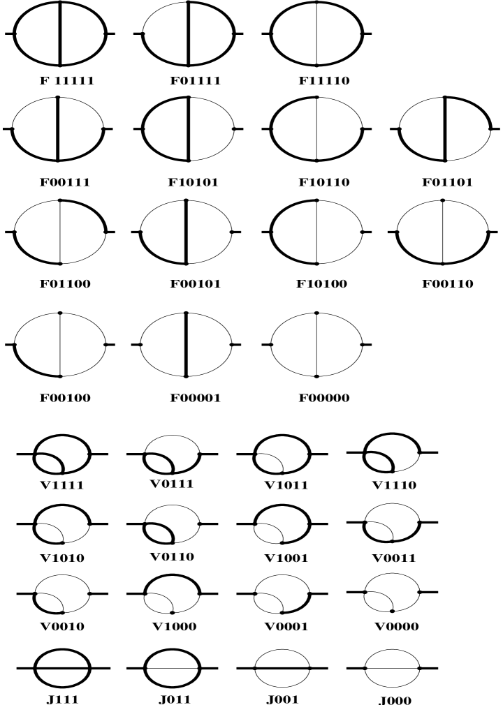
Figure 2: The full set of two-loop self-energies diagrams with one mass. Bold and thin lines correspond to the mass and massless propagators, respectively.

We consider here the following master-integrals in Euclidean space-time with dimension $D=4-2\varepsilon$:

$${\bf ONS}\{{\cal IJ}\}(i,j,m) \equiv K^{-1}\int d^{D}kP^{(i)}(k,{\cal I}m)\left.P^{(j)}(k-p,{\cal J}m)\right|_{p^{2}=-m^{2}},$$

$${\bf J}\{{\cal IJK}\}(i,j,k,m) \equiv K^{-2}\int d^{D}k_{1}d^{D}k_{2}P^{(i)}(k_{1},{\cal I}m)P^{(j)}(k_{1}-k_{2},{\cal J}m)$$

$$~{}~{}~{}~{}~{}\times\left.P^{(k)}(k_{2}-p,{\cal K}m)\right|_{p^{2}=-m^{2}},$$

$${\bf V}\{{\cal IJKL}\}(i,j,k,l,m) \equiv K^{-2}\int d^{D}k_{1}d^{D}k_{2}P^{(i)}(k_{2}-p,{\cal I}m)$$

$$\times P^{(j)}(k_{1}-k_{2},{\cal J}m)P^{(k)}(k_{1},{\cal K}m)\left.P^{(l)}(k_{2},{\cal L}m)\right|_{p^{2}=-m^{2}},$$

$${\bf F}\{{\cal ABIJK}\}(a,b,i,j,k,m) \equiv m^{2}K^{-2}\int d^{D}k_{1}d^{D}k_{2}P^{(a)}(k_{1},{\cal A}m)P^{(b)}(k_{2},{\cal B}m)$$

$$\times P^{(i)}(k_{1}-p,{\cal I}m)$$

$$\times P^{(j)}(k_{2}-p,{\cal J}m)\left.P^{(k)}(k_{1}-k_{2},{\cal K}m)\right|_{p^{2}=-m^{2}},$$

where

$$K=\frac{\Gamma(1+\varepsilon)}{\left(4\pi\right)^{\frac{D}{2}}\left(m^{2}\right)^{\varepsilon}},~{}~{}~{}P^{(l)}(k,m)\equiv\frac{1}{(k^{2}+m^{2})^{l}},$$

the normalization factor $1/(2\pi)^{D}$ for each loop is assumed, and ${\cal A,B,I,J,K}=0,1.$

The finite part of most of the F-type master-integrals can be obtained from results of Ref.[14] in the limit $z\rightarrow 1$. F10101 and F11111 have been calculated in Refs.[78, 79], respectively. Instead of the usually taken F01101 integral [78, 80] we consider J111 as master integral. We recall the results of all master integrals for completeness. The last master integral F00111 has been found in [75].

The finite part of the integrals of V- and J-type can be found in Refs.[81]. The calculation of some $\sim\varepsilon$ and $\sim\varepsilon^{2}$ parts of master integrals of this type have been performed by DEM.

The results for F-type master-integrals are follows:

$${\bf F}\{{\cal ABIJK}\}(1,1,1,1,1,m)=a_{1}\zeta(3)+a_{2}\frac{\pi}{\sqrt{3}}S_{2}+a_{3}i\pi\zeta(2)+{\cal O}(\varepsilon),$$ (32)

and the coefficients $\{a_{i}\}$ are given in Table I:

$$\begin{array}[]{|c|c|c|c|c|c|c|c|c|}\hline\cr\vrule\lx@intercol\hfil TABLE~{}~{}~{}I\hfil\lx@intercol\vrule\lx@intercol\\ \hline\cr&{\bf F11111}&{\bf F00111}&{\bf F10101}&{\bf F10110}&{\bf F01100}&{\bf F00101}&{\bf F10100}&{\bf F00001}\\[8.5359pt] \hline\cr a_{1}&1&0&-4&-1&0&-3&-2&-3\\[8.5359pt] \hline\cr a_{2}&-\frac{9}{2}&9&\frac{27}{2}&9&\frac{27}{2}&\frac{27}{2}&9&0\\[8.5359pt] \hline\cr a_{3}&0&0&\frac{1}{3}&0&1&1&\frac{2}{3}&1\\[8.5359pt] \hline\cr\end{array}$$

where [82, 78, 77]

$$S_{2}=\frac{4}{9\sqrt{3}}{\rm Cl}_{2}\left(\frac{\pi}{3}\right)=0.260434137632\cdots.$$

Here we used the $m^{2}-i\varepsilon$ prescription. The results for the remaining master integrals are the following ones:

$${\bf V}\{{\cal IJKL}\}(1,1,1,1,m)=\frac{1}{2\varepsilon^{2}}+\frac{1}{\varepsilon}\left(\frac{5}{2}-\frac{\pi}{\sqrt{3}}\right)+\frac{19}{2}+\frac{b_{1}}{2}\zeta(2)-4\frac{\pi}{\sqrt{3}}-\frac{63}{4}S_{2}$$

$$+ \hskip-8.0pt\frac{\pi}{\sqrt{3}}\ln 3+\varepsilon\Biggl{\{}\frac{65}{2}+b_{2}\zeta(2)-b_{3}\zeta(3)-12\frac{\pi}{\sqrt{3}}-63S_{2}+b_{4}\zeta(2)\ln 3+\frac{9}{4}b_{4}S_{2}\frac{\pi}{\sqrt{3}}$$

$$+ \frac{63}{4}S_{2}\ln 3+4\frac{\pi}{\sqrt{3}}\ln 3-\frac{1}{2}\frac{\pi}{\sqrt{3}}\ln^{2}3-\frac{b_{5}}{2}\frac{\pi}{\sqrt{3}}\zeta(2)-\frac{21}{2}\frac{{\rm Ls}_{3}\left(\frac{2\pi}{3}\right)}{\sqrt{3}}\Biggr{\}}+{\cal O}(\varepsilon^{2}),$$

where the coefficients $\{b_{i}\}$ are listen in Table II :

$$\begin{array}[]{|c|c|c|c|c|c|}\hline\cr\vrule\lx@intercol\hfil TABLE~{}~{}~{}II\hfil\lx@intercol\vrule\lx@intercol\\ \hline\cr&b_{1}&b_{2}&b_{3}&b_{4}&b_{5}\\[8.5359pt] \hline\cr{\bf V1111}&-1&-6&\frac{9}{2}&4&9\\[8.5359pt] \hline\cr{\bf V1001}&3&8&-\frac{3}{2}&0&21\\[8.5359pt] \hline\cr\end{array}$$

$${\bf J111}(1,1,1,m) = -m^{2}\Biggl{(}\frac{3}{2\varepsilon^{2}}+\frac{17}{4\varepsilon}+\frac{59}{8}+\varepsilon\Biggl{\{}\frac{65}{16}+8\zeta(2)\Biggr{\}}$$ (33)

$$- -\varepsilon^{2}\Biggl{\{}\frac{1117}{32}-52\zeta(2)+48\zeta(2)\ln 2-28\zeta(3)\Biggr{\}}+{\cal O}(\varepsilon^{3})\Biggr{)},$$

$${\bf J011}(1,1,2,m) = \frac{1-4\varepsilon}{2(1-2\varepsilon)(1-3\varepsilon)}\Biggl{(}\frac{1}{\varepsilon^{2}}+2\frac{\pi}{\sqrt{3}}-\frac{2}{3}\zeta(2)$$ (34)

$$+ \varepsilon\Biggl{\{}8\frac{\pi}{\sqrt{3}}-\frac{2}{3}\zeta(2)-6\frac{\pi}{\sqrt{3}}\ln 3+\frac{2}{3}\zeta(3)+27S_{2}\Biggr{\}}+{\cal O}(\varepsilon^{2})\Biggr{)},$$

$${\bf J011}(1,1,1,m) = -\frac{m^{2}}{2}\frac{4-15\varepsilon}{(1-2\varepsilon)(1-3\varepsilon)(2-3\varepsilon)}\Biggl{(}\frac{1}{\varepsilon^{2}}+\frac{3}{2}\frac{\pi}{\sqrt{3}}$$ (35)

$$+ \varepsilon\Biggl{\{}\frac{45}{8}\frac{\pi}{\sqrt{3}}-\frac{9}{2}\frac{\pi}{\sqrt{3}}\ln 3+\frac{81}{4}S_{2}\Biggr{\}}$$

$$+ \varepsilon^{2}\Biggl{\{}12-\zeta(2)-\frac{1863}{16}S_{2}-\frac{867}{32}\frac{\pi}{\sqrt{3}}+\frac{207}{8}\frac{\pi}{\sqrt{3}}\ln 3+\frac{243}{4}S_{2}\ln 3$$

$$- \frac{27}{4}\frac{\pi}{\sqrt{3}}\ln^{2}3-21\frac{\pi}{\sqrt{3}}\zeta(2)-\frac{81}{2}\frac{{\rm Ls}_{3}\left(\frac{2\pi}{3}\right)}{\sqrt{3}}\Biggr{\}}+{\cal O}(\varepsilon^{3})\Biggr{)},$$

$${\bf ONS11}(1,1,m) = \frac{1}{1-2\varepsilon}\Biggl{[}\frac{1}{\varepsilon}-\frac{\pi}{\sqrt{3}}+\varepsilon\left\{\frac{\pi}{\sqrt{3}}\ln 3-9S_{2}\right\}$$

$$+ \varepsilon^{2}\left\{9S_{2}\ln 3-\frac{1}{2}\frac{\pi}{\sqrt{3}}\ln^{2}3-6\frac{{\rm Ls}_{3}\left(\frac{2\pi}{3}\right)}{\sqrt{3}}-3\frac{\pi}{\sqrt{3}}\zeta(2)\right\}+{\cal O}(\varepsilon^{3})\Biggr{]},$$

where [77]

$${\rm Ls}_{3}(x)=-\int_{0}^{x}\ln^{2}\left|2\sin\frac{\theta}{2}\right|d\theta~{}~{}\mbox{ and }~{}~{}{\rm Ls}_{3}\left(\frac{2\pi}{3}\right)=-2.14476721256949\cdots$$

The above results were checked numerically. Padé approximants were calculated from the small momentum Taylor expansion of the diagrams [84]. The Taylor coefficients were obtained by means of the package [85] with the master integrals taken from [86]. Further we made use of the idea of Broadhurst [87] to apply the FORTRAN program PSLQ [88] to express the obtained numerical values in terms of a ‘basis’ of irrational numbers, which were predicted by DEM.

Let us point out that the numbers we obtain are related to polylogarithms at the sixth root of unity and hence are in the same class of transcendentals obtained by Broadhurst [87] in his investigation of three-loop diagrams which correspond to a closure of the two-loop topologies considered here.

Acknowledgments.

Author would like to express his sincerely thanks to the Organizing Committee of the PNPI Winter School for the kind invitation, the financial support, and for fruitful discussions.

Author is supported in part by INTAS grant 00-366. He thanks also the Alexander von Humboldt Foundation for its support at the beginning of the study.

References

-
[1]
V.A. Smirnov, Phys.Lett. B460 (1999) 397;
J.B. Tausk, Phys.Lett. B469 (1999) 225;
C. Anastasiou, et al., Nucl.Phys. B (Proc.Suppl.) 89 (2000) 262. - [2] T. Gehrmann and E. Remiddi, Nucl.Phys. B580 (2000) 485.
-
[3]
V.A. Smirnov, Phys.Lett. B491 (2000) 130; Phys.Lett.
B500 (2001) 3;
C. Anastasiou, et al., Nucl.Phys. B565 (2000) 445;
T. Gehrmann and E. Remiddi, Nucl.Phys. B601 (2001) 248, Nucl.Phys. B601 (2001) 287. - [4] T. Gehrmann and E. Remiddi, in: Proceedings of the 3th International symposium on Radiative Corrections (RADCOR-2000), Carnel, USA (hep-ph/0101147).
- [5] V.A. Smirnov, DESY preprint DESY 01-190 (hep-ph/0111160).
- [6] K.G. Chetyrkin, A.L. Kataev and F.V. Tkachov, Nucl.Phys. B174 (1980) 345.
-
[7]
W. Celmaster and R.J. Gonzalves,
Phys.Rev. D21 (1980) 3112;
A.Terrano, Phys.Lett. B93 (1980) 424;
B. Lampe and G. Kramer, Phys.Scr. 28 (1986) 585. -
[8]
K.G. Chetyrkin and V.A. Smirnov,
Phys.Lett. B144 (1984) 419;
K.G. Chetyrkin, in: AIHENP 93, Proceedings of the 3th International Workshop on Software Engineering, Artificial Intelligence and Expert Systems, ed.by K.-H. Becks and D. Perret-Gallix, p. 523. - [9] A.V. Kotikov, Phys.Lett. B375 (1996) 240; in: Proceedings of the XVth International Workshop “High Energy Physics and Quantum Field Theory“ (hep-ph/0102177).
- [10] D.I. Kazakov and A.V. Kotikov, Theor.Math.Phys. 73 (1987) 1264.
- [11] D.I. Kazakov and A.V. Kotikov, Nucl.Phys. B307 (1988) 721; B345 (1990) 299(E);
- [12] A.V.Kotikov, Theor.Math.Phys. 78 (1989) 134.
- [13] D.I. Kazakov and A.V. Kotikov, Phys.Lett. B291 (1992) 171.
- [14] J. Fleischer, A.V. Kotikov, and O.L. Veretin, Nucl.Phys. B547 (1999) 343.
- [15] J. Fleischer, A.V. Kotikov, and O.L. Veretin, Phys.Lett. B417 (1998) 163.
- [16] J. Fleischer, A.V. Kotikov, and O.L. Veretin, Acta Phys.Polon. B29 (1998) 2611, hep-ph/9808243.
- [17] A.V. Kotikov, Phys.Lett. B254 (1991) 158; Mod.Phys.Lett. A6 (1991) 677.
- [18] A.V. Kotikov, Phys.Lett. B259 (1991) 314; Mod.Phys.Lett. A6 (1991) 3133.
- [19] A.V. Kotikov, Phys.Lett. B267 (1991) 123; B295 (1992) 409(E); Int.J.Mod.Phys. A7 (1992) 1977.
- [20] A.V. Kotikov, JHEP 9809 (1998) 001; in: ACAT 2000, Proceedings of the 7th International Workshop on Software Engineering, Artificial Intelligence and Expert Systems, ed.by D. Perret-Gallix, in American Institute of Physics Press., (hep-ph/0011316); in: Proceedings of the XVth International Workshop “High Energy Physics and Quantum Field Theory“ (hep-ph/0102178).
-
[21]
G. Passarino,
in: Proceedings of the ICHEP2000, Osaka, 2000 (hep-ph/0009249);
in: Proceedings of a Symposium in honor of Prof. Sirlin, 2000
(hep-ph/0101299);
G. Passarino and S. Uccirati, hep-ph/0112004. - [22] S. Laporta, Phys.Lett. B504 (2001) 188; Int.J.Mod.Phys. A15 (2000) 5087; hep-ph/0111123.
- [23] L. Durand, P.M. Fishbane and L.M. Simmons, J.Math.Phys. 17 (1976) 1973.
- [24] D.J. Broadhurst and A.V. Kotikov, Phys.Lett. B441 (1998) 345.
- [25] W.N.Bailey, Generalized Hypergeometrical series, New York, 1972.
- [26] A.N. Vasil’ev, Yu.M. Pis’mak and J.R. Honkonen, Theor.Math.Phys. 46 (1981) 104; 47 (1981) 465.
- [27] D.I. Kazakov, Theor.Math.Phys. 58 (1984) 223; Phys.Lett. B133 (1983) 406.
- [28] D.Broadhurst and J.A.Gracey, preprint OUT-4102-46,1993.
- [29] D.I. Kazakov, Theor.Math.Phys. 62 (1985) 84.
-
[30]
A.N.Vasil’ev, S.E.Derkachov, N.A.Kivel and A.S.Stepanenko,
Theor.Math.Phys. 94 (1993) 127;
V.A. Kivel, A.S. Stepanenko and A.N. Vasil’ev, Nucl.Phys. B424 (1994) 619;
A.N.Vasil’ev and A.S.Stepanenko, Theor.Math.Phys. 94 (1993) 471; Theor.Math.Phys. 97 (1993) 1349. - [31] J.A. Gracey, Phys.Lett. B262 (1991) 49; Int.J.Mod.Phys. A9 (1994) 567, Int.J.Mod.Phys. A9 (1994) 727.
- [32] V.S. Fadin, R. Fiore and M.I. Kotsky, Phys.Lett. B387 (1996) 593.
- [33] A.P.Prudnikov, Yu.A.Brychkov and O.I.Marichev, Integrals and series, Vol.3, New-York, 1990.
- [34] A.V. Kotikov, JETP Lett. 58 (1993) 731.
-
[35]
T. Appelquist et al., Phys.Rev. D33 (1986) 3774;
Phys.Rev.Lett. 60 (1988) 2575;
D. Nash, Phys.Rev. Lett. 62 (1989) 3024. - [36] I.N. Kondrashuk and A.V. Kotikov, Phys.Rev. D53 (1996) 2260.
- [37] S.H. Park, Phys.Rev. D45 (1992) 3332.
- [38] A.V. Kotikov and L.N. Lipatov, Nucl.Phys. B582 (2000) 19.
- [39] A.V. Kotikov and L.N. Lipatov, in: Proceedings of the XXXV Winter School, Repino, S’Peterburg, 2001 (hep-ph/0112346).
-
[40]
A.N. Vasil’ev, Yu.M. Pis’mak and J.R. Honkonen,
Theor.Math.Phys. 50 (1982) 127;
W. Bernrenther and F. Wegner, Phys.Rev.Lett. 57 (1986) 1383. -
[41]
A.M. Polyakov,
JETP Lett. 12 (1970) 381;
M. D’Eramo, L. Peliti, G. Parisi, Lett. Nuovo Cim. 2 (1971) 878;
E. S. Fradkin and M. Palchik, Phys.Rept. 44 (1978) 249. -
[42]
V.S. Fadin and L.N. Lipatov, Phys. Lett.
B429 (1998) 127;
G. Camici and M. Ciafaloni, Phys. Lett. B430 (1998) 349. - [43] D.J. Broadhurst, J.A. Gracey, and D. Kreimer, Z.Phys. C75 (1997) 559.
- [44] L. Euler, Novi Comm.Acad.Sci.Petropol. 20 (1775) 140.
-
[45]
D. Zagier, in: Proc. First European Congress Math., Birkhäuser,
Boston, 1994, Vol II, pp 497-512;
D. Borwein, J.M. Borwein and R. Girgensohn, Proc.Edin.Math.Soc. 38 (1995) 273;
J.M. Borwein, D.A. Bradley and D.J. Broadhurst, Preprint CECM-96-067, OUT-4102-63 (hep-th/9611004);
J.M Borwein, D.J. Broadhurst, and J. Kamnitzer, Preprint OUT-4102-88, CECM-99-13, 1999 (hep-th/0004153);
M.E. Hoffman, The algebra of multiple harmonic series, preprint from Mathematics Department, U.S. Naval Academy, Annapolis (1996);
D.J. Broadhurst, Open University preprint OUT-4102-65, 1996 (hep-th/9612012). - [46] D.I. Kazakov and A.V. Kotikov, Sov. J. Nucl. Phys. 46 (1987) 1057 [Yad. Fiz. 46 (1987) 1767].
- [47] A.V. Kotikov, G. Parente and O.A. Sampayo, Phys. Lett. B328 (1994) 374.
- [48] D.I. Kazakov, A.V. Kotikov, G. Parente, O.A. Sampayo and J. Sanchez Guillen, Phys. Rev. Lett. 65 (1990) 1535.
- [49] W.L. van Neerven and E.B. Zijlstra, Phys. Lett. B272 (1991) 127; Phys. Lett. B273 (1991) 476; Nucl. Phys. B383 (1992) 525.
- [50] A.V. Kotikov, A.V. Lipatov, G. Parente and N.P. Zotov, Preprint US-FT/7-01 (hep-ph/0107135).
- [51] E.G. Floratos, C. Kounnas, and R. Lacage, Nucl. Phys. B192 (1981) 417.
- [52] A.V. Kotikov, Phys. Atom. Nucl. 57 (1994) 133; Phys. Rev. D49 (1994) 5746.
- [53] V.G. Krivokhizhin et al., Z. Phys. C36 (1987) 51; Z. Phys. C48 (1990) 347.
-
[54]
V.I. Vovk, Z. Phys. C47 (1990) 57;
A.V. Kotikov, G. Parente and J. Sanchez Guillen, Z. Phys. C58 (1993) 465. - [55] A.V. Kotikov and V.G. Krivokhijine, in Proceedings of International Workshop on Deep Inelastic Scattering and Related Phenomena (1998), Brussels (hep-ph/9805353); V.G. Krivokhijine and A.V. Kotikov, JINR preprint E2-2001-190 (hep-ph/0108224).
- [56] G. Parente, A.V. Kotikov and V.G. Krivokhizhin, Phys. Lett. B333 (1994) 190.
- [57] A.L. Kataev, A.V. Kotikov, G. Parente and A.V. Sidorov, Phys. Lett. B388 (1996) 179; Phys. Lett. B417 (1998) 374; Nucl. Phys. Proc. Suppl. 64 (1998) 138, hep-ph/9709509.
- [58] A.L. Kataev, G. Parente and A.V. Sidorov, Nucl. Phys. B573 (2000) 405; Preprint CERN-TH/2001-58 (hep-ph/0106221)
-
[59]
F. Martin, Phys. Rev. D19 (1979) 1382;
C. Lopez and F.I. Yndurain, Nucl. Phys. B171 (1980) 231; Nucl. Phys. B183 (1981) 157;
A.V. Kotikov, Phys. Atom. Nucl. 56 (1993) 1276. - [60] A.V. Kotikov et al., Theor. Math. Phys. 84 (1990) 744; Theor. Math. Phys. 111 (1997) 442.
- [61] L. L. Jenkovszky, A. V. Kotikov and F. Paccanoni, Sov. J. Nucl. Phys. 55 (1992) 1224;. JETP Lett. 58 (1993) 163; Phys. Lett. B 314(1993) 421.
- [62] A.V. Kotikov and G. Parente, Nucl. Phys. B549 (1999) 242; Nucl. Phys. (Proc. Suppl.) 99 (2001) 196, hep-ph/0010352; in Proc. of the Int. Conference PQFT98 (1998), Dubna (hep-ph/9810223); in Proc. of the 8th Int. Workshop on Deep Inelastic Scattering, DIS 2000 (2000), Liverpool, p. 198 (hep-ph/0006197).
-
[63]
A. De Rújula et al.,
Phys.Rev. D10 (1974) 1649;
R.D. Ball and S. Forte, Phys.Lett. B336 (1994) 77;
L. Mankiewicz, A. Saalfeld and T. Weigl, Phys.Lett. B393 (1997) 175. - [64] A.V. Kotikov, Mod. Phys. Lett. A11 (1996) 103; Phys.Atom.Nucl. 59 (1996) 2137.
-
[65]
H. Abramowitz, E.M. Levin, A. Levy, and U. Maor,
Phys. Lett. B269 (1991) 465;
A. Levy, DESY preprint 95-003 (1995) (hep-ph/9501346). - [66] A.V. Kotikov, JETP Lett. 59 (1994) 1; Phys.Lett. B338 (1994) 349.
-
[67]
S. Keller, M. Miramontes, G. Parente, J. Sanchez-Guillen,
and O.A. Sampayo, Phys.Lett. B270 (1990) 61;
L.H. Orr and W.J. Stirling, Phys.Rev.Lett. B66 (1991) 1673;
E. Berger and R. Meng, Phys.Lett. B304 (1993) 318. -
[68]
A.V. Kotikov, JETP Lett. 59 (1994) 667;
A.V. Kotikov and G. Parente, Phys.Lett. B379 (1996) 195. -
[69]
K. Prytz, Phys.Lett. B311 (1993) 286;
A.M. Cooper-Sarkar et al., Z. Phys. C39 (1988) 281. -
[70]
A.V. Kotikov, JETP 80 (1995) 979;
A.V. Kotikov and G. Parente, Mod. Phys. Lett. A12 (1997) 963; JETP 85 (1997) 17; in Proc. of the Int. Workshop on Deep Inelastic Scattering, DIS96 (1996), Rome, p. 237 (hep-ph/9608409). -
[71]
F.V. Tkachov,
Phys.Lett. B100 (1981) 65;
K.G. Chetyrkin and F.V. Tkachov, Nucl.Phys. B192 (1981) 159; - [72] C. Ford, I. Jack and D.R.T. Jones, Nucl.Phys. B387 (1992) 373.
- [73] J. Fleischer, M. Tentyukov and O.V. Tarasov, Nucl.Phys.Proc.Suppl. 89 (2000) 112.
- [74] E. Remiddi, Nuovo Cim. A110 (1997) 1435.
- [75] J. Fleischer, M.Yu. Kalmykov, and A.V. Kotikov, Phys.Lett. B462 (1999) 169; B467 (1999) 310(E).
-
[76]
J. Fleischer, M.Yu. Kalmykov, and A.V. Kotikov, in AIHENP 99,
Proceedings of the 6th International Workshop on Software Engineering,
Artificial Intelligence and Expert Systems, ed.by
G. Athanasiu and D. Perret-Gallix, in Parisianou S.A., Athens, 2000,
pp. 231-237, (hep-ph/9905379);
J. Fleischer and M.Yu. Kalmykov, Comput.Phys.Commun. 128 (2000) 531; Phys.Lett. B470 (1999) 168;
A.I. Davydychev, Phys.Rev. D61 (2000) 087701; -
[77]
L. Lewin,
Polylogarithms and Associated
Functions, North Holland, New-York, 1981;
A. Devoto and D.W. Duke, Riv. Nuovo Cim. 7 (1984) 1;
N. Nilsen, Nova Acta 90 (1909) 125;
K.S. Kolbig, J.A. Mignaco and E. Remiddi, BIT 10 (1970) 38; Nuovo Cim. A11 (1972) 824. - [78] D.J. Broadhurst, Z.Phys. C47 (1990) 115.
- [79] V. Borodulin and G. Jikia, Phys.Lett. B391 (1997) 434.
-
[80]
N. Gray, D.J. Broadhurst, W. Grafe and K. Schilcher, Z.Phys. C48
(1990) 673;
D.J. Broadhurst, N. Gray and K. Schilcher, Z.Phys. C52 (1991) 111;
D.J. Broadhurst, Z.Phys. C54 (1992) 599. -
[81]
A. Djouadi, Nuovo Cim. A100 (1988) 357;
P.N. Maher, L. Durand and K.Riesselmann, Phys.Rev. D48 (1993) 1061; Phys.Rev. D52 (1995) 553(E):
R. Scharf and J.B. Tausk, Nucl.Phys. B412 (1994) 523; F.A. Berends, M. Buza, M. Böhm and R. Scharf, Z.Phys. C63 (1994) 227;
F.A. Berends and J.B. Tausk, Nucl.Phys. B421 (1994) 456;
S. Bauberger, F.A. Berends, M. Böhm and M. Buza, Nucl.Phys. B434 (1995) 383. -
[82]
J. van der Bij and M. Veltman, Nucl.Phys. B231 (1984) 205;
F. Hoogeveen, Nucl.Phys. B259 (1985) 19;
J. van der Bij and F. Hoogeveen, Nucl.Phys. B283 (1987) 477. - [83] A.I. Davydychev and M.Yu. Kalmykov, Nucl.Phys.Proc.Suppl. 89 (2000) 283; Nucl.Phys. B605 (2001) 266.
-
[84]
J. Fleischer and O.V. Tarasov,
Z.Phys. C64 (1994) 413;
O.V. Tarasov, Nucl.Phys. B480 (1996) 397. - [85] L.V. Avdeev, J. Fleischer, M.Yu. Kalmykov and M.N. Tentyukov, Nucl.Inst.Meth. A389 (1997) 343; Comp.Phys.Commun. 107 (1997) 155.
- [86] A.I. Davydychev and J.B. Tausk, Nucl.Phys. B397 (1993) 123.
- [87] D.J. Broadhurst, Eur.Phys.J. C8 (1999) 311.
-
[88]
H.R.P. Ferguson, D.H. Bailey and S. Arno, NASA-Ames Technical Report,
NAS-96-005;
D.H. Bailey and D.J. Broadhurst, math.NA/9905048.