SNUTP 01-046

Self-tuning Solution of Cosmological Constant in RS-II Model and Goldstone Boson

Jihn E. Kim

Department of Physics and Center for Theoretical Physics, Seoul National University, Seoul 151-747, Korea

I give a review on the self-tuning solution[2] of the cosmological constant in a 5D RS-II model using a three index antisymmetric tensor field $A_{MNP}$. The three index antisymmetric tensor field can be the fundamental one appearing in 11D supergravity. Also, the dual of its field strength $H_{MNPQ}$, being a massless scalar, may be interpreted as a Goldstone boson of some spontaneously broken global symmetry.

PRESENTED AT

COSMO-01
Rovaniemi, Finland,
August 29 – September 4, 2001

1 Introduction

The cosmological constant problem is the most severe hierarchy problem or fine-tuning problem known to particle physicists since 1975[3, 4].

Another well-known hierarchy problem is the gauge hierarchy problem encountered in GUT. In GUT’s there appear two scales which differ by a factor of $10^{28}$. At the classical Lagrangian level, there appear parameters of the GUT scale which is of order $10^{32}$ GeV². But the loop corrections and GUT symmetry breaking must be considered. The known hierarchy requires the difference must be of order $\sim$TeV² after including all these effects, i.e. $M_{1}^{2}+M_{2}^{2}=O(10^{-28})$ GeV². To achieve this small number, we have to fine-tune the parameters $M_{1}^{2}$ and $M_{2}^{2}$ both of which appear in the Lagrangian. Supersymmetry has been employed to understand this gauge hierarchy problem.

Gravity is described by the metric tensor $g_{\mu\nu}$. The Rieman tensor $R_{\mu\nu}$ is the other second rank tensor. The Einstein equation is obtained by the variation of the action proportional to $\int d^{4}x\sqrt{-g}R$, where $g$ is the determinant of the metric and $R=g^{\mu\nu}R_{\mu\nu}$. But a general form of the action invariant under the general coordinate transformation can be written as

$$S=\int d^{4}x\sqrt{-g}\left\{\frac{M^{2}}{2}R-V_{0}+\cdots\right\}$$ (1)

where $M^{2}$ is proportional to the inverse Newton constant $G$ ($M^{2}=8\pi/G$), $V_{0}$ is a pure constant and the ellipses denote the other pieces in the Lagrangian whose vacuum expectation value(VEV) vanishes. The variation of the above action leads to the gravity equation

$$R_{\mu\nu}-\frac{1}{2}Rg_{\mu\nu}-8\pi GV_{0}g_{\mu\nu}=8\pi GT_{\mu\nu}$$ (2)

where the energy momentum tensor $T_{\mu\nu}$ is obtained from the ellipses. The term $8\pi GV_{0}$ is the so-called cosmological constant(c.c.) $\Lambda$. Historically, Einstein introduced the cosmological constant in 1917 to make the universe static, which was the belief at that time. But the observation of the Hubble expansion twelve years later invalidated Einstein’s need for the c.c. As we have seen in Eq. (1), it is quite natural to introduce a constant in the action. Therefore, the c.c. problem could have been formulated in 1910’s, 60 years earlier. The constant is of order the mass scale in question. The parameter $M$ appearing in Eq. (1) is the Planck mass $M=2.44\times 10^{18}$ GeV which is astronomically larger than the electroweak scale. Since gravity introduces a large mass $M$, any other parameter in gravity is expected to be of that order, which is a natural expectation. Namely, $V_{0}$ appearing in (1) is expected to be of order $M$. However, the bound on the vacuum energy was known to be $<(0.01\ {\rm eV})^{4}$, which implied a fine-tuning of order $10^{-120}$. Thus, c.c. problem has been known to be the most serious hierarchy problem.

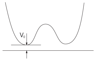
Figure 1: The Higgs potential for breaking the $SU(2)\times U(1)$ gauge group.

Usually, a hierarchy problem is understood if there exists a symmetry related to it. The difficulty with the c.c. problem is that there is no such symmetry working. An obvious symmetry one can imagine is the scale invariance. However it must be badly broken by the mass terms at the electroweak scale. If the scale invariance is assumed to be broken at the electroweak scale, we still have a hierarchy problem of order $10^{56}$.

This c.c. problem surfaced as a very serious one when one considered the spontaneous symmetry breaking in particle physics [3]. As shown in Fig. 1, one does not know whehere to put the minimum point. Except gravity, the position does not matter. But in gravity its position determines the c.c. There have been several attempts toward the solution, by Hawking[5], Witten[6], Weinberg[7], Coleman[8], etc, under the name of probabilistic interpretation in Euclidian gravity, boundary of different phases, anthropic solution, wormhole solution, etc. We will comment more on Hawking’s solution later. The anthropic solution relies on the requirement that life evolution is not very much affected by the existence of c.c. However, if c.c. is too large, galaxy formations may be hindered. Weinberg observed that the requirement for the condensation of matter needs $\rho_{\Lambda}<550\rho_{c}$. Thus, we may need a fine-tuning but only one part in a thousand.

2 Self-tuning solutions

2.1 Old version

If there exists a solution for the flat space, it is called a self-tuning solution, or a solution with the undetermined integration constant(UIC). In 4D, it is impossible. For a nonzero $\Lambda$ in 4D, a flat space ansatz $ds^{2}=d{\bf x}^{2}-dt^{2}$ does not allow a solution. The de Sitter space(dS, $\Lambda>0$) or anti de Sitter space(AdS, $\Lambda<0$) solution is possible. To reach a nearly flat space solution, one needs an extreme fine tuning, which is the c.c. problem.

But suppose that there exists an UIC. Witten used the four index field strength $H_{\mu\nu\rho\sigma}$ to obtain an UIC[6]. The equation of motion of $H$ leads to an UIC, say $c$. Thus, the vacuum energy contains a piece $\sim c^{2}$. This UIC $c$ can be adjusted so that the final c.c. is zero. Once $c$ is determined, there is no more UIC because $H_{\mu\nu\rho\sigma}$ is not a dynamical field in 4D. When vacuum energy is added later, there is no handle to adjust further. In a sense, it was another way of fine-tuning. However, if there exists a dynamical field allowing an UIC, it is a desired old style self-tuning solution. This old version did not care whether there also exist de Sitter or anti de Sitter solutions. Selection of the flat space out of these solutions is from a principle such as Hawking’s probabilistic choice.

2.2 New version

In recent years, a more ambitious attempt was proposed, where only the flat space ansatz has the solution[9]. This idea attracted a great deal of attention in the Randall-Sundrum II type models[10]. The RS type models were constructed in 5D anti de Sitter space, i.e. the 5D bulk cosmological constant $\Lambda_{b}<0$, with brane(s) located at fixed point(s). The RS II model uses only one brane. At this brane one can introduce a brane tension $\Lambda_{1}$. Thus, the gravity Lagrangian contains two free parameters $\Lambda_{b}$ and $\Lambda_{1}$.

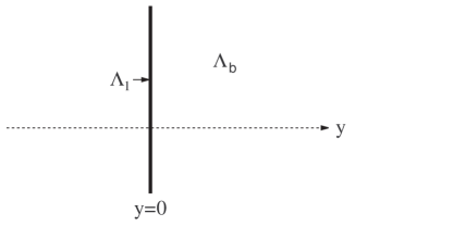
Figure 2: The RS II model with a brane at $y=0$.

In Fig. 2, we show this situation schematically, where the extra dimension is the $y$-direction. The 4D is denoted as $x^{\mu}$. The 4D flat space ansatz allows a solution for a specific choice of $k_{1}$(basically $\Lambda_{1}$, $k_{1}=\Lambda_{1}/6M^{3}$) and $k$(basically $\Lambda_{b}$, $k=\sqrt{-\Lambda_{b}/6M^{3}}$): $k_{1}=k$. Therefore, it requires a fine-tuning between parameters as in the 4D case. However, it seems to be an improvement since we reach at the 4D flat space from nonzero cosmological constants and the RS II type models seems to be a good play ground to obtain UIC solutions.

The RS II model is an interesting extension of the space-time without compactification. With the bulk AdS, the uncompactified fifth dimension can be acceptable due to the localized gravity. For the brane located at $y=0$, the action is

$$S=\int d^{4}x\int dy\sqrt{-g}\left\{\frac{M^{3}}{2}(R-\Lambda_{b})+(-\Lambda_{1}+{\cal L}_{matter})\delta(y)\right\}$$ (3)

where $M$ is the 5D fundamental scale and ${\cal L}_{matter}$ is the matter Lagrangian, assuming the matter is located at the brane only. The flat space ansatz,

$$ds^{2}=\beta(y)^{2}\eta_{\mu\nu}dx^{\mu}dx^{\nu}+dy^{2}$$ (4)

allows the solution if $k=k_{1}$. Even though the 4D is flat, it is curved in the direction of the fifth dimension, denoted by the warp factor $\beta(y)=\beta_{0}\exp(-k|y|)$. Namely, the gravity is exponentially unimportant if one is far away from the brane. [If there were more branes, there are more conditions to satisfy toward a flat space solution since one can introduce a brane tension at each brane. Thus, the RS II type models are the simplest ones.]

The try to obtain a new type of self-tuning solution was initiated by Arkani-Hamed et. al. and Kachru et. al.[9]. For example the 5D Lagrangian with the introduction of a massless bulk scalar field $\phi$, coupling to the brane tension,

$${\cal L}=R-\Lambda e^{a\phi}-\frac{4}{3}(\nabla\phi)^{2}-Ve^{b\phi}\delta(y)$$ (5)

where we set $M^{3}/2=1$. We may ask, $``$Why this Lagrangian?”, which involves more difficult related questions. Accepting this, we must satisfy the following Einstein and field equations, with the flat ansatz (4),

$$({\rm dilaton}) : \frac{8}{3}\phi^{\prime\prime}+\frac{32}{3}A^{\prime}\phi^{\prime}-a\Lambda e^{a\phi}-bV\delta(y)e^{b\phi}=0$$

$$(55) : 6(A^{\prime})^{2}-\frac{2}{3}(\phi^{\prime})^{2}+\frac{1}{2}\Lambda e^{a\phi}=0$$

$$(55),(\mu\nu) : 3A^{\prime\prime}+\frac{4}{3}(\phi^{\prime})^{2}+\frac{1}{2}e^{b\phi}V\delta(y)=0$$ (6)

where $2A(y)=\ln\beta(y)$, and prime denotes the derivative with respect to $y$. For $\Lambda=0$, there exists a bulk solution satisfying $A^{\prime}=\alpha\phi^{\prime}$,

$$\phi=\pm\frac{3}{4}\ln\left|\frac{4}{3}y+c\right|+d,\ \ \alpha=\pm\frac{1}{3}$$ (7)

where $c$ and $d$ are determined without fine-tuning of the parameters. The solution has a singularity at $y_{c}\equiv-(3/4)c$ or diverges logarithmically at large $|y|$. The logarithmically diverging solution does not realize the localization of gravity. If we restrict the space up to the singular point $y_{c}$, then at every $y$ inside the space it is flat. However, the effective 4D theory is the one after integrating out the allowed $y$ space. Since $y_{c}$ is the naked singularity, we do not know how to cut the $y$ integration near $y_{c}$, implying a possibility that the flat space ansatz does not lead to a solution. Depending on how to cut the integral, one may introduce a nonzero c.c. F$\ddot{\rm o}$rste et. al. tried to understand this problem by curing the singularity by putting a brane at $y_{c}$[11]. Then, a flat 4D space solution is possible but one needs a fine-tuning. It is easy to understand. If one more brane is introduced, then there is one more tension parameter $\Lambda_{2}$, i.e. in the Lagrangian one adds $\Lambda_{2}\delta(y-y_{c})$. If the space is flat for one specific value of $\Lambda_{2}$, then it must be curved for the other values of $\Lambda_{2}$, since the $y$ integration gives a c.c. contribution directly from $\Lambda_{2}$.

This example teaches us that the self-tuning solution better should not have a singular point in the whole $y$ space.

3 The self-tuning solution with $1/H^{2}$

As we have seen in the RS II model, the Einstein-Hilbert action alone does not produce a self-tuning solution. Inclusion of higher order gravity does not improve this situation[12]. We need matter field(s) in the bulk. The first try is a massless spin-0 field in the bulk as Ref. ([9]) tried so that it affects the whole region of the bulk. However, it may be better if there appears a symmetry in the spin-0 sector. These are achieved by a three index antisymmetric tensor field $A_{MNP}$. In 5D the dual of its field strength is interpreted as a scalar. The field strength $H_{MNPQ}$ is invariant under the gauge transformation $A_{MNP}\rightarrow A_{MNP}+\partial[M\lambda_{NP}]$, thus masslessness arises from the symmetry. There will be one $U(1)$ gauge symmetry remaining with one massless pseudoscalar field which is $a$, $\partial_{M}a\propto\sqrt{-g}\epsilon_{MNPQR}H^{NPQR}$. But the interactions are important for the solution, as Ref. ([9]) find a bulk solution for the specific form of the interaction.

The first guess is the bulk term $-(M/48)H^{2}$ where $H^{2}\equiv H_{MNPQ}H^{MNPQ}$. The brane with tension $\Lambda_{1}$ is located at $y=0$, and the bulk c.c. is $\Lambda_{b}$. The ansatze for the solution are

$${\rm Ansatz\ 1}\ :\ ds^{2}=\beta(y)^{2}\eta_{\mu\nu}dx^{\mu}dx^{\nu}+dy^{2},\ \ {\rm Ansatz\ 2}\ :\ H_{\mu\nu\rho\sigma}=\epsilon_{\mu\nu\rho\sigma}\frac{\sqrt{-g}}{n(y)}$$ (8)

where $\mu,\cdots$ are the 4D indices, and $n(y)$ is a function of $y$ to be determined. It is sufficient to consider (55) and ($\mu\nu$) components Einstein equations and the $H$ field equation. By setting $M=1$, we obtain the bulk solution

$$\Lambda_{b}<0\ : \ \beta(|y|)=(\frac{a}{k})^{1/4}[\pm\sinh(4k|y|+c)]^{1/4}$$

$$\Lambda_{b}>0\ : \ \beta(|y|)=(\frac{a}{k})^{1/4}[\sin(4k|y|+c^{\prime})]^{1/4}$$

$$\Lambda_{b}=0\ : \ \beta(|y|)=|4a|y|+c^{\prime\prime}|^{1/4}.$$ (9)

For a localizable (near $y=0$) metric, there exists a singularity at $y=-c/4k$, etc., except for some cases with $\Lambda_{b}>0$. Thus, for these singular cases another brane is necessary to cure the singularity, and we need a fine-tuning as in the case of Kachru et. al.[9]. The bulk de Sitter space without a singularity is worth commenting. Such a solution is periodic and depicted in Fig. 3. We can consider only $|y|\leq y_{c}$, then $\beta^{\prime}=0$ at $y=\pm y_{c}$. The boundary condition at $y=0$ determines $c^{\prime}=\cot^{-1}(k_{1}/k)$ and the boundary condition at $y_{c}$ determines $y_{c}$ such that $c^{\prime}=4ky_{c}-\cot^{-1}(k_{2}/k)$, so it looks like an UIC. But for $y_{c}$ to behave like an undetermined integration constant, it should not appear in the equations of motion. Note, however, that $y_{c}$ is the VEV of the radion $g_{55}$, and hence it cannot be a strictly massless Goldstone boson. If it were massless, it will serve to the long range gravitational interaction and hence give different results from the general relativity predictions in the light bending experiments. Therefore, it should obtain a mass and hence $y_{c}$ is not a free parameter but fixed. So the boundary condition at $y_{c}$ is a fine-tuning condition[14].

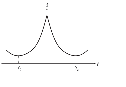
Figure 3: The flat space solution with $H^{2}$.

In the remainder of this talk, I present a working self-tuning model. Let us consider the $1/H^{2}$ term,

$$S=\int d^{4}x\int dy\sqrt{-g}\left(\frac{1}{2}R+\frac{2\cdot 4!}{H^{2}}-\Lambda_{b}-\Lambda_{1}\delta(y)\right).$$ (10)

3.1 Flat space solution

For the flat space ansatze, we use

$$ds^{2}=\beta(y)^{2}\eta_{\mu\nu}dx^{\mu}dx^{\nu}+dy^{2},\ \ H_{\mu\nu\rho\sigma}=\epsilon_{\mu\nu\rho\sigma}\frac{\sqrt{-g}}{n(y)},\ \ H_{5\mu\nu\rho}=0.$$ (11)

The $H$ field equation is $\partial_{M}[\sqrt{-g}H^{MNPQ}/H^{4}]=\partial_{\mu}[\sqrt{-g}H^{\mu NPQ}/H^{4}]=0$, and hence fixes $n$ as a function of $y$ only. The two relevant Einstein equations are

$$(55)\ : \ 6\left(\frac{\beta^{\prime}}{\beta}\right)^{2}=-\Lambda_{b}-\frac{\beta^{8}}{A}$$

$$(\mu\nu)\ : \ 3\left(\frac{\beta^{\prime}}{\beta}\right)^{2}+3\left(\frac{\beta^{\prime\prime}}{\beta}\right)=-\Lambda_{b}-\Lambda_{1}\delta(y)-3\left(\frac{\beta^{8}}{A}\right)$$ (12)

where $\Lambda_{b}<0$ and $2n^{2}=\beta^{8}/A$ with $A>0$. We require the $Z_{2}$ symmetry, and the bulk equation is easily solved. The boundary condition at $y=0$ is $\beta^{\prime}/\beta|_{0^{+}}=-\Lambda_{1}/6$. Then, we find a solution

$$\beta(|y|)=\frac{(k/a)^{1/4}}{\left[\cosh(4k|y|+c)\right]^{1/4}}$$ (13)

where

$$k=\sqrt{\frac{-\Lambda_{b}}{6}},\ \ a=\sqrt{\frac{1}{6A}},\ \ k_{1}=\frac{\Lambda_{1}}{6}.$$ (14)

The flat solution is shown in Fig. 4.

Figure 4: The flat space solution.

This solution has the integration constants $a$ and $c$. $a$ is basically the charge of the universe and determines the 4D Planck mass. $c$ is the UIC which is fixed by the boundary condition at $y=0$,

$$\tanh(c)=\frac{k_{1}}{k}=\frac{\Lambda_{1}}{\sqrt{-6\Lambda_{b}}}.$$ (15)

This solution shows that, for any value of $\Lambda_{1}$ in the finite region allowing $\tanh$, it is possible to have a flat space solution. Even if the observable sector adds some constant to $\Lambda_{1}$, still it is possible to have the flat space solution, just by changing the shape little bit via $c$. The change is acceptable since $H$ is a dynamical field. Note that $\beta(y)$ is a decreasing function of $|y|$ in the large $|y|$ region and it goes to zero exponentially as $|y|\rightarrow\infty$. This property is needed for a self-tuning solution.

The key points found in our solution are
(i) $\beta$ has no singularity: Our solution extends to infinity without singularity, and $\beta^{\prime}\rightarrow 0$ as $y\rightarrow\infty$.
(ii) 4D Planck mass is finite: Even if the extra dimension is not compact, this theory can describe an effective 4D theory since gravity is localized. Integrating with respect to $y$, we obtain an effective 4D Planck mass which is finite

$$M^{2}_{4D\ Planck}=\int_{-infty}^{\infty}dy\beta^{2}=2M^{3}\sqrt{\frac{k}{a}}\int_{0}^{\infty}\frac{1}{[\cosh(4ky+c)]^{1/2}}dy$$ (16)

and is expected to be of order the fundamental parameters.
(iii) Self-tuning: We obtained a self-tuning solution. To check that the 4D c.c. is zero we integrate out the solution. For that we have to include the surface term also

$$S_{surface}=\int d^{4}xdy4\cdot 4!\partial_{M}[\sqrt{-g}\frac{H^{MNPQ}A_{NPQ}}{H^{4}}].$$ (17)

Then the action is

$$S=\int d^{4}xdy\sqrt{-\eta}\beta^{4}\left[\frac{1}{2\beta^{2}}R_{4}-4\frac{\beta^{\prime\prime}}{\beta}-6\left(\frac{\beta^{\prime}}{\beta}\right)^{2}-\Lambda_{b}+\frac{2\cdot 4!}{H^{2}}-\Lambda_{1}\delta(y)\right]+S_{surface}.$$ (18)

Then, $-\Lambda_{4D}$ is the $y$ integral except the $R_{4}$ term. One can show that $\Lambda_{4D}=0$ and it is consistent with the original ansatz of the flat space[2].

3.2 De Sitter and anti de Sitter space solutions

For the de Sitter and anti de Sitter space solutions, the metric is assumed as

$$ds^{2}=\beta(y)^{2}g_{\mu\nu}dx^{\mu}dx^{\nu}+dy^{2}$$

$$g_{\mu\nu}=diag.\left(-1,e^{2\sqrt{\lambda}t},e^{2\sqrt{\lambda}t},e^{2\sqrt{\lambda}t}\right),\ \ (dS_{4}\rm\ background\ with\ \lambda>0)$$

$$g_{\mu\nu}=diag.\left(-e^{2\sqrt{-\lambda}x_{3}},e^{2\sqrt{-\lambda}x_{3}},e^{2\sqrt{-\lambda}x_{3}},1\right),\ \ (AdS_{4}\rm\ background\ with\ \lambda<0).$$ (19)

Note that $k=\sqrt{-\Lambda_{b}/6},k_{1}=\Lambda_{1}/6$, and the 4D Riemann tensor is $R_{\mu\nu}=3\lambda g_{\mu\nu}$. The (55) and (00) components equations are

$$6\left(\frac{\beta^{\prime}}{\beta}\right)^{2}-6\lambda\frac{1}{\beta^{2}}=-\Lambda_{b}-3\frac{\beta^{8}}{A}$$

$$3\left(\frac{\beta^{\prime}}{\beta}\right)^{2}+3\frac{\beta^{\prime\prime}}{\beta}-3\lambda\frac{1}{\beta^{2}}=-\Lambda_{b}-\Lambda_{1}\delta(y)-3\frac{\beta^{8}}{A}.$$ (20)

The 4D c.c. obtained from the above ansatze is $\lambda$. Since we cannot obtain the solution in closed forms, we cannot show this by integration. However, we have checked this kind of behavior[2] in the RS II model, using the Karch-Randall form[13]. Here, we show just that the de Sitter and anti de Sitter space solutions exist, and show the warp factor numerically. In our model, the $y$ derivative of the metric is

$$\beta^{\prime}=\pm(k_{\lambda}^{2}+k^{2}\beta^{2}-a^{2}\beta^{10})^{1/2},\ \ k_{\lambda}=(\lambda)^{1/2}$$ (21)

At $y=y_{h}$ where $\beta(y_{h})=0$, $\beta^{\prime}(y_{h})$ needs not be zero due to the presence of the nonvanishing $k_{\lambda}$. Therefore, there exists a point $y_{h}$ where $\beta^{\prime}$ is finite. It is the de Sitter space horizon. It takes an infinite amount of time to reach $y_{h}$. Also, we can see that it is possible $\beta$ can be nonzero where $\beta^{\prime}$ is zero. It is the anti de Sitter space solution. These Anti de Sitter space and de Sitter space solutions are shown in Figs. 5 and 6. For the de Sitter space, we can integrate from $-y_{h}$ to $+y_{h}$. As in the Karch-Randall example, it should give the 4D c.c. $\lambda$. The AdS solution does not give a localized gravity.

Figure 5: The anti de Sitter space solution.

Figure 6: The de Sitter space solution.

In the presence of de Sitter and anti de Sitter space solutions, the c.c. problem relies on the old self-tuning solution. Namely, the c.c. is probably zero, following Hawking[5]. Hawking showed that in 4D, with the Euclidian space action

$$-S_{E}=-\frac{1}{2}\int d^{4}x\sqrt{+g}[(R+2\Lambda)+(1/48)H_{\mu\nu\rho\sigma}H^{\mu\nu\rho\sigma}]$$ (22)

where we use the unit $8\pi G=1$. The Einstein equation and field equations are

$$R_{\mu\nu}-(1/2)g_{\mu\nu}R=\Lambda g_{\mu\nu}-T_{\mu\nu}$$

$$\partial_{\mu}[\sqrt{g}H^{\mu\nu\rho\sigma}]=0.$$

From the field equation, one has $H^{\mu\nu\rho\sigma}=(1/\sqrt{g})\epsilon^{\mu\nu\rho\sigma}c$ or $H^{2}=4!c^{2}$. Thus, he obtained $T^{\mu\nu}=-\Lambda_{H}g^{\mu\nu},\Lambda_{H}=-c^{2}/2,R=-4\Lambda_{eff},\Lambda_{eff}=\Lambda+\Lambda_{H}$. Thus,

$$-S_{E}=-(1/2)\int d^{4}x\sqrt{g}(R+2\Lambda_{eff})={\rm Volume}\cdot(\Lambda+\Lambda_{H})=\frac{3M^{4}}{\Lambda_{eff}}$$ (23)

which is maximum at $\Lambda_{eff}=0^{+}$ which is shown in Fig. 5.

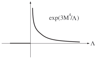
Figure 7: Hawking’s probability

Note that Hawking used equations of motion. Duff, on the other hand, used the action itself to calculate the Euclidian action, and obtained $-S_{E}=3M^{4}(\Lambda-(3/2)c^{2})/(\Lambda-(1/2)c^{2})^{2}$ which is minimum at $0^{+}$[15]. But the consideration of the surface term in the action would give additional contribution and should give Hawking’s result. The surface term is essential as we have shown in our self-tuning solution.

Thus, the maximum probability occurs when the c.c. is zero. Our self-tuning solution relies on this probabilistic choice of the flat one from the flat, de Sitter and anti de Sitter space solutions.

4 Goldstone boson scenario?

One point to consider is whether the peculiar kinetic energy term can be made sensible. Actually we can construct an example which has reasonable terms. Let us introduce a $U(1)$ gauge field strength $F_{MN}$ and its coupling to $H_{MNPQ}$ as

$$-\frac{1}{8}H^{2}(F^{2})^{2}-\frac{1}{4}F^{2}.$$ (24)

The Gaussian integral of $A_{M}$ would choose $F^{2}=-1/H^{2}$, and we would obtain the desired $1/H^{2}$ term. Therefore, consideration of $1/H^{2}$ can be meaningful. But the question is why there is no term with $H^{2}$ in the first place.

Since $H$ is a massless boson, it can be considered as a Goldstone boson. Thus, one may try to construct a theory where a pseudoscalar Goldstone boson is a kind of cosmion, self-tuning the c.c. at zero. The question is how one obtains the term $1/H^{2}$ instead of $H^{2}$.

References

- [1]
- [2] J. E. Kim, B. Kyae, and H. M. Lee, Phys. Rev. Lett. 86 (2001) 4223 [hep-th/0011118] and Nucl. Phys. B613 (2001) 306 [hep-th/0101027].
- [3] M. Veltman, Phys. Rev. Lett. 34 (1975) 777.
- [4] S. Weinberg, Rev. Mod. Phys. 61 (1989) 1.
- [5] S. Hawking, Phys. Lett. B134 (1984) 403; E. Baum, Phys. Lett. B138 (1983) 185.
- [6] E. Witten, in Proc. Shelter Island II Conference, ed. R. Jackiw, H. Khuri, S. Weinberg, and E. Witten (Shelter Island 1983, MIT Press 1985), p.369. For an earlier use of , see, A. Aurila, H. Nicolai, and P. K. Townsend, Nucl. Phys. B176 (1980) 509.
- [7] S. Weinberg, Phys. Rev. Lett. 59 (1987) 2607.
- [8] S. Coleman, Nucl. Phys. B310 (1988) 643.
- [9] N. Arkani-Hamed, S. Dimopoulos, N. Kaloper, and R. Sundrum, Phys. Lett. B480 (2000) 193 [hep-th/0001197]; S. Kachru, M. Shultz, and E. Silverstein, Phys. Rev. D62 (2000) 045021 [hep-th/0001206].
- [10] L. Randall and R. Sundrum, Phys. Rev. Lett. 83 (1999) 4690 [hep-th/9906064].
- [11] Frste, Z. Lalak, and H. P. Nilles, Phys. Lett. B481 (2000) 360 [hep-th/0002164]; JHEP 0009 (2000) 034 [hep-th/0006139].
- [12] J. E. Kim, B. Kyae, and H. M. Lee, Phys. Rev. D62 (2000) 045013 [hep-ph/9912344] and Nucl. Phys. B582 (2000) 296 [hep-th/0004005].
- [13] A. Karch and L. Randall, [hep-th/0011156].
- [14] J. E. Kim, B. Kyae and H. M. Lee, hep-th/0110103.
- [15] M. Duff, Phys. Lett. B226 (1989) 36.