Gluon Interactions with Color-Neutral Fields

We investigate the interactions of color neutral fields with gluons in the regge region, and propose a model in which the field strength of the gluons couples to these fields. This model yields to first order in perturbation theory a structure function which coincides with that obtained in deep inelastic scattering (in the Double Log Approximation of QCD) to first order at low $q$ with a correction. We propose that higher order corrections in this model will contribute to the parton structure functions beyond the DLA. It is also shown that the Born approximation in this model yields a potential having a monopole, and a quadrupole term that may couple to hadronic currents providing angular momentum transitions of $\triangle J=2,0$, as is the case in hadron regge trajectories.

1 Introduction

The regge region of QCD poses a great challenge for particle physicists to this day. Although great strides in the hard a and semi-hard regions [2] have been made, the former sector is still obscure. The source of the challenge lies in the complexity of QCD in the IR region, namely the non- perturbative sector of QCD when momentum exchanges $q$ are that of the order of $\Lambda_{QCD}$. One immediate consequence of this complexity is the inability to describe fundamental interactions among hadrons using perturbation theory. To mention a few are hadron resonances, hadron diffraction dissociation, and hadron structure (which should have a very rich description when the coupling between constituent quarks and gluons is very strong). It is also worth while mentioning that many of these processes are dominated by an exchange of a color singlet, or what is known as the Pomeron which has become an entire sub-field of QCD. This problem has received great attention [4, 2, 3, 6], and remains elusive because of its non-perturbative description.

Probably one of the most notable achievements of QCD is asymptotic freedom [1]. This of course enables perturbation to be extremely effective in the high energy regime, and is especially effective in treating the scattering object (which is always a color neutral field) as made up of an ensemble of very lightly interacting partons. Thus one can neglect the interactions among the various partons within a particular field, and only worry about the interactions those partons have with fields on which they scatter from. Of course as one drops in energy one loses this nice picture, and compositeness has to be taken into account. However, here too asymptotic freedom (or the inverse of it) can be utilized. Since at lower energies the partons interact very strongly it is more sensible to treat this ensemble of constituent fields as one effective color-neutral field (CNF) while enabling it to interact with constituent fields that do carry color (such as gluons). In this description a composite color-neutral field can be viewed as an effective field [2] composed of partons whose life time is much greater than their interaction time. This says that effectively one is in the region where exchanged momenta between partons is much greater than the mass of the entire neutral field, or simply put:

$$\frac{1}{q_{parton}}\approx\triangle t_{int^{\prime}ofparton}\ll\triangle t_{life}\approx\frac{1}{m_{CNF}}.$$

These scales define to what extent one can treat a composite field as an effective quantum field without worrying about the vary difficult problems of specifying interactions between the partons themselves, let alone their individual interactions with any external (gluon) fields. It is evident that such a description would be particularly useful in a case where CNFs interact at low exchanged momenta (in the IR region) where the scale of the interaction may be of the same order as of the masses of the CNFs. One can now avoid the description among the various partons (since these will occur at a different higher scale), and still treat the CNF as a composite field. If the CNF were to interact with any color-carrying field, then to first order the CNF may be treated as neutral parton which must remain neutral at least for a time by which the interactions take place, namely the life time of the color-neutral field $\bigtriangleup t_{life}$. In essence this scheme enables treating interactions of non-local composite fields in the IR region without specifying the local interactions that take place between constituent fields such quarks and gluons. However it is important to remember that once the scale of the interactions between the various partons is equal to the scale of the neutral quantum field, such a description is not useful, and a new scale must be chosen. One therefore expects that any physical observable obtained from such a description is valid only within the confines of the scales chosen.

2 CNF-Gauge Boson Vertex

We propose a model in which a color-neutral field interacts with two color carrying gauge bosons. Two gauge particles are needed as a minimum to preserve the color-neutrality of the CNF. Of course this isn’t the only interaction possible that could fulfill this requirement since one could also have interactions of two CNFs’ with multiple gauge fields. However as we shall argue such interactions are suppressed significantly.

With this said, amplitudes between in and out states of two CNFs’ and two gauge bosons (see fig.(1)) must fulfill the following two requirements: the first is due to spin statistics of the gauge bosons for which the amplitude must satisfy the following permutation:

$$A^{\mu\nu}_{ab}(k_{1},k_{2})=A^{\nu\mu}_{ba}(k_{2},k_{1}).$$

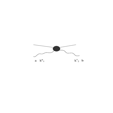
Figure 1: The CNF-gauge boson vertex

The second is due to current conservation which dictates that the amplitude should have the Ward identity,

$$k_{1\mu}A^{\mu\nu}_{ab}=k_{2\nu}A^{\mu\nu}_{ab}=0.$$

These two conditions are suffice to constrain the general form of such an amplitude to the following:

$$A^{\mu\nu}_{ab} \sim \delta_{ab}\Bigg{[}F_{0}\left(g^{\mu\nu}k_{1}\cdot k_{2}-k_{1}^{\nu}k_{2}^{\mu}\right)$$ (1)

$$+ F_{1}\left(q^{\mu}-k_{1}^{\mu}\left(\frac{q\cdot k_{1}}{k_{1}^{2}}\right)\right)\left(q^{\nu}-k_{2}^{\nu}\left(\frac{q\cdot k_{2}}{k_{2}^{2}}\right)\right)\Bigg{]}.$$

with $q^{\mu}=k_{1}^{\mu}-k_{2}^{\mu}$.

Since the amplitude above really represents a color neutral current then it follows that $F_{0}$, and $F_{1}$ are associated with the structure functions of the CNF. The amplitude (1) says that $F_{1}$ should vanish as $q$ gets small. In fact the term proportional to $F_{1}$ becomes relevant at high $q$. In such a scenario, our assumption of having the momentum of the interaction of the CNF with any external field not being comparable to the momentum of the interactions between the partons (which make up the CNF) may be compromised. As was indicated, when these two scales are of the same order our description of a CNF becomes invalid. In light of this we shall focus only the term proportional to $F_{0}$ in what is to follow.

In searching for a field theoretical model which would give rise to such a structure of the scattering amplitude, a particular gauge invariant term added to the total Lagrangian of the non-abelian gauge theory fulfills the above requirements, and is given by

$${\mathcal{L}}_{CNF-g}=\bar{\psi}\Bigg{(}\frac{\lambda}{2}{\mathcal{F}}^{\mu\nu}_{ab}{\mathcal{F}}_{\nu\mu ab}+...+\frac{\lambda_{n}}{2+2n}\Big{(}{\mathcal{F}}^{\mu\nu}_{ab}{\mathcal{F}}_{\nu\mu ab}\Big{)}^{n}\Bigg{)}\psi.$$ (2)

Where ${\mathcal{F}}^{\mu\nu}_{ab}$ is the field strength of the gauge field and $\psi$ is a color neutral field.

Of course apart from one of the first term in (2) this interaction does not directly produce the kind of interaction given in (1), but yields for the $n^{\rm{th}}$ term $3+2n$ vertices each having two CNFs and $\gamma(1+n)$ ($\gamma=2,3,4$) gauge fields. Because (2) is manifestly gauge invariant, for each vertex in each term of (2) one can integrate out $\gamma(1+n)-2$ gauge fields to produce (1). So really it is only the first term in (2) that is relevant since the other terms are proportional to it up to a coupling constant, which could as well be redefined. We shall not present a formal proof to this claim, but instead provide an argument based on dimensional analysis for why we can neglect higher order terms in (2).

The coupling $\lambda_{n}$ has dimensions of $(mass_{\rm{CNF}})^{-(d+4n)}$, where $d$ depends on the space-time properties of the field (for example $d=3$ for a spinor field while for a scalar field $d=2$), while the mass has a natural cut-off scale at $\Lambda_{QCD}$. The negative mass dimension of the coupling indicates that at high momentum transfer (2) is comprised of what are so called irrelevant operators [8]. It can be seen from (2) that the $n^{\rm{th}}$ amplitude is proportional (in the $t$-channel) to $\sim\left(\frac{\sqrt{t}}{\Lambda_{QCD}}\right)^{d+4n}$, which means they drop as $t$ goes down. As a consequence it is apparent that

$$(A_{ab}^{\mu\nu})_{n+1}=\left(\frac{\sqrt{t}}{\Lambda_{QCD}}\right)^{4}(A_{ab}^{\mu\nu})_{n}.$$

If the term in parenthesis above is small to begin with then the $n^{\rm{th}}+1$ amplitude will be significantly dwarfed from the previous one. Hence for small $t$ it is suffice to consider the first term in the series of (2). This argument also establishes that the more gluons appear in vertices with CNFs, the faster those amplitudes associated with these vertices will vanish. Therefore the vertex with the minimum amount of gluons (which is two) would give the largest contribution to the total amplitude. The first term in (2) is also of particular interest (as will be shown) when the CNF can be described by a ‘manyfield’ [5], one which could describe a collection of states that have different spin (like a regge trajectory). This term may facilitate transitions between states that differ in angular momentum $\triangle J=2,0$ in the Born approximation.

3 QCD Corrections to CNF-Gluon Vertex

Given the first term in (2) we seek to evaluate the amplitudes of the following process:

$$\rm{CNF}+g\rightarrow\rm{CNF}+g.$$

We wish to evaluate corrections to this process that are first order in $\lambda$, and in $\alpha_{s}$ . There are five relevant terms in the perturbation series contributing to the correction of the vertex given by the first term of (2), and are described by the Feynman diagrams shown in figures (2a-2e). These contributions can be grouped into two categories: the first (figs. (2a-2c)) are terms that result in the reduction of the three gluon vertex, and the four gluon vertex to a two gluon vertex respectively. These will be shown to have no physical relevance since they exactly correspond to integrating out the extra gluon fields as discussed in section (2). The second group (figs. (2d, 2e)) do have a physical contribution, and are ‘genuine’ QCD corrections which contribute to $F_{0}$.

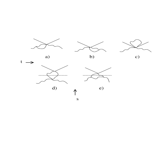
Figure 2: First order corrections to the CNF-gluon vertex

We compute these amplitudes by scaling the gauge field by the familiar prescription $A^{\mu}\rightarrow gA^{\mu}$, and anticipate the strong coupling to show in propagators. For these corrections it is also assumed that the CNFs are scalars, however this can be generalized to a CNF of any spin without affecting the results that follow from our calculations.

Since we are interested in terms proportional to $F_{0}$ it is worth while to put the external gluons on shell since this will eliminate terms proportional to $k_{1}^{\mu},k_{2}^{\nu}$, and leave only terms proportional to $k_{1}^{\nu},k_{2}^{\mu}$ as in (1). For the first group of diagrams (in the Feynman gauge figs. (2a-2c)) this will introduce a ‘temporary’ infra-red divergence for which the off-shell gluons are assigned a fictitious mass.

The first of these is given by:

$$ic_{1~{}ab}^{\mu\nu}=-\frac{\lambda}{4}4\pi\int\frac{d^{d}k}{(2\pi)^{d}}\alpha_{s}\Gamma^{\mu\sigma\rho}_{acd}(k_{1},k)\frac{g^{\sigma\sigma^{\prime}}\delta_{cc^{\prime}}}{k^{2}-\mu^{2}}\times$$

$$\frac{g^{\rho\rho^{\prime}}\delta_{dd^{\prime}}}{(k-k_{1})^{2}-\mu^{2}}\Gamma^{\rho^{\prime}\sigma^{\prime}\nu}_{c^{\prime}d^{\prime}b}(k_{1},k_{2},k),$$ (3)

where $\Gamma$ [8] is the familiar $SU(N)$ triple gauge boson vertex.

Since diagrams contributing the running of $\alpha_{s}$ have been omitted (after all these are also first order in $\alpha_{s}$) a legitimate questions is raised on whether the expression for the running of $\alpha_{s}$ should be included in (3), and thus integrated out. The answer to this question depends on the structure of the diagram. As can be seen from figure (2a), the off-shell propagators are directly connected to the vertex (1). Thus, varying the strong coupling implies a variation in $\lambda$, or simply put $\lambda=\lambda(\alpha_{s}(k))$. This in itself is a true statement (this is evident from (2) when the gauge field is unscaled by $g$), though a variation of $k$ implies a variation in $\lambda$ which would be inappropriate at this stage since we are performing perturbation to first order in $\lambda$ where it is assumed to be constant; hence $\alpha_{s}$ is constant as well. This argument applies to all but the fifth diagram.

Having cleared this issue (3) is given by:

$$ic_{1~{}ab}^{\mu\nu} = -\delta_{ab}\frac{N\lambda\alpha_{s}}{4}4\pi\int^{1}_{0}dx\int\frac{dl^{d}}{(2\pi)^{d}}\frac{-3(g^{\mu\nu}k_{1}\cdot k_{2}-k_{1}^{\nu}k_{2}^{\mu})+2g^{\mu\nu}(\frac{1-d}{d})l^{2}}{(l^{2}-\mu^{2})^{2}}$$ (4)

$$= i\delta_{ab}\frac{\pi N\lambda\alpha_{s}}{(4\pi)^{\frac{d}{2}}}g^{\mu\nu}(1-d)\left(\frac{1}{\mu^{2}}\right)^{1-\frac{d}{2}}$$

$$+ i\delta_{ab}\frac{3\pi N\alpha_{s}}{4(4\pi)^{\frac{d}{2}}}(g^{\mu\nu}k_{1}\cdot k_{2}-k_{1}^{\nu}k_{2}^{\mu})\Gamma\left(2-\frac{d}{2}\right)\left(\frac{1}{\mu^{2}}\right)^{2-\frac{d}{2}}.$$

The second amplitude (fig. (2b)) $c_{2~{}ab}^{\mu\nu}$ is obtained from $c_{1~{}ab}^{\mu\nu}$ on interchanging $k_{1}\rightarrow k_{2}$, $\mu\rightarrow\nu$, and $a\rightarrow b$. The latter is symmetric upon these interchanges hence $c_{2~{}ab}^{\mu\nu}=c_{1~{}ab}^{\mu\nu}$.

Evaluating the third amplitude (fig. 2c) we get:

$$ic_{3~{}ab}^{\mu\nu} = -\frac{N\alpha_{s}\delta_{ab}}{2}\int\frac{d^{d}k}{(2\pi)^{d}}\frac{(d-1)g^{\mu\nu}}{k^{2}-\mu^{2}}$$ (5)

$$= i\frac{2\pi N\alpha_{s}\delta_{ab}}{(4\pi)^{\frac{d}{2}}}g^{\mu\nu}(d-1)\left(\frac{1}{\mu^{2}}\right)^{1-\frac{d}{2}}$$

.

Summation on the first three terms gives:

$$\sum^{3}_{i}c_{i~{}ab}^{\mu\nu}=\frac{3N\alpha_{s}}{8\pi}\bigtriangleup_{ab}^{\mu\nu}(k_{1},k_{2})\left(\frac{2}{\epsilon}-\log{\mu^{2}}-\gamma+\log{4\pi}\right)$$ (6)

where $\bigtriangleup_{ab}^{\mu\nu}(k_{1},k_{2})=\delta_{ab}(g^{\mu\nu}k_{1}\cdot k_{2}-k_{1}^{\nu}k_{2}^{\mu})$.

This sum suffers from the familiar ultraviolet divergences, however it does not depend on any dynamical variables and therefore does not contribute to $F_{0}$, at least not to first order in $\alpha_{s}$. One can subtract these divergences by redefining $\lambda$ with counter terms, and impose the following condition:

$$F_{0}(t=t_{o},\mu\rightarrow 0)=\lambda,$$ (7)

where $F_{0}$ is given by:

$$F_{0}(t,\mu)=\frac{\epsilon_{a\mu}\epsilon_{b\nu}}{G(k_{1},k_{2})}\left(\lambda\bigtriangleup^{\mu\nu}(k_{1},k_{2})+\sum^{5}_{i}c_{i~{}ab}^{\mu\nu}(t,\mu)\right)+\delta F_{0},$$ (8)

with $G(k_{1},k_{2})=\epsilon^{a}_{\mu}\epsilon^{b}_{\nu}\bigtriangleup_{ab}^{\mu\nu}(k_{1},k_{2})$, and $t_{o}$ being a renormalization scale chosen at some momentum exchange.

The function $F_{0}$ is a CNF structure function obtained from pure QCD processes, and includes contributions from all five diagrams, while the term $\delta F_{0}$ contains the appropriate counter terms.

Proceeding to evaluate the second group of diagrams we note that unlike the first three the former  (fig (2d,2e)) are most easily obtained (especially in the regge region) using $s$-channel unitarity, namely the Cutkosky cutting rules [9]. Once the $s$-channel amplitude is obtained, one then can use crossing symmetry to get the $t$-channel amplitude which presently is of most interest.

According to the cutting rules each diagram  (figs. (2d, 2e)) is split into two tree level amplitudes; one giving the process of $g+g\rightarrow g+g$, the other giving the process of $g+g\rightarrow\rm{CNF+CNF}$.

One can now evaluate the imaginary part for the fourth and fifth amplitudes using these cuts to give:

$${\mathcal{I}}m(c_{i~{}ab}^{\mu\nu})_{s-channel} = \frac{g^{4}}{2}\sum_{g}\int\frac{d^{4}u}{(2\pi)^{3}}\frac{d^{4}u^{\prime}}{(2\pi)^{3}}\delta(u^{2})\delta(u^{\prime 2})(2\pi)^{4}\delta^{4}(k_{1}+k_{2}-u_{i}-u_{i}^{\prime})$$ (9)

$$\times (Y_{abcd}^{\mu\nu\sigma\rho})_{i}(\epsilon_{\sigma c}\epsilon_{\sigma^{\prime}c^{\prime}}\epsilon_{\rho~{}d}\epsilon_{\rho^{\prime}~{}d^{\prime}})(X_{c^{\prime}d^{\prime}}^{\rho^{\prime}\sigma^{\prime}})_{i}^{\dagger},$$

where $u_{i},u^{\prime}_{i}$ are the momenta of the out-going gluons for each diagram respectively, and the sum is over gluon polarizations.

The terms $Y_{i},X_{i}$ are the scattering amplitudes of the $g,g$, and $g,CNF$ processes respectively. For the fourth amplitude these tree level expressions are given by:

$$(Y^{\rho\sigma\mu\nu}_{abcd})_{4} = \frac{-1}{g^{2}}(\Gamma_{4})^{\rho\sigma\mu\nu}_{abcd}(k_{1},k_{2},u^{\prime}_{4},u_{4})$$ (10)

$$(X^{\rho^{\prime}\sigma^{\prime}}_{c^{\prime}d^{\prime}})_{4} = \lambda\bigtriangleup^{\rho^{\prime}\sigma^{\prime}}_{c^{\prime}d^{\prime}}(u^{\prime}_{4},u_{4}),$$ (11)

where $\Gamma_{4}$ is the familiar four gluon vertex, and $u_{4}=\frac{k_{1}+k_{2}}{2}-k$, $u^{\prime}_{4}=\frac{k_{1}+k_{2}}{2}+k$.

While for the fifth amplitude the tree level expressions are:

$$(Y_{abcd}^{\mu\nu\sigma\rho})_{5} = 4\pi\alpha_{s}\Gamma^{\mu\sigma\lambda}_{aec}\Gamma^{\hskip 1.42271pt\nu\rho}_{\lambda\hskip 1.42271ptbed}\left(\frac{1}{k^{2}}\right)$$ (12)

$$(X_{c^{\prime}d^{\prime}}^{\rho^{\prime}\sigma^{\prime}})_{5} = \lambda\bigtriangleup^{\rho^{\prime}\sigma^{\prime}}_{d^{\prime}c^{\prime}}(u^{\prime}_{5},u_{5}),$$ (13)

where $u_{5}=k_{1}-k$, $u^{\prime}_{5}=k_{2}+k$.

Working in the center of mass frame with the in-coming gluons momenta given by:

$$k_{1}=(\frac{\sqrt{s}}{2},\frac{\sqrt{s}}{2},0,0)\hskip 28.45274ptk_{2}=(\frac{\sqrt{s}}{2},-\frac{\sqrt{s}}{2},0,0),$$

it is convenient to parameterize the vector $k$ with Sudakov variables:

$$k^{\mu}=\alpha k^{\mu}_{1}+\beta k^{\mu}_{2}+{\mathbf{k}}.$$ (14)

This parametization is particularly convenient where soft interactions (regge region) in the $t$-channel take place since they make $k$ predominantly transverse, and that implies $\alpha,\beta\ll 1$. In what follows this enables second order terms in these variables to be neglected.

With this methodology one notices that in the case of $(c_{4ab}^{\mu\nu})_{s-channel}$ neither amplitudes of the cut diagram (fig. (2d)) contains any off-shell gluon propagators, and all gluons are on shell. Hence this amplitude is most easily obtained using a physical gauge [10] where a gluon has two independent degrees of freedom with two polarization vectors that obey the following relation:

$$\sum_{G}\epsilon^{\mu}\epsilon^{\nu}=d_{\perp}^{\mu\nu},$$ (15)

and the sum is over gluon polarizations.

The tensor $d^{\mu\nu}_{\perp}$ is the transverse metric $(0,0,-1,-1)$. This tensor is obtained when the polarization vectors of the gauge fields in (9) are chosen to be purely along the transverse plane with respect to the in-coming gluon momenta.

Utilizing this gauge freedom, implementing (9), and keeping only first order terms in Sudakov parameters the imaginary amplitude of $(c_{4ab}^{\mu\nu})_{s-channel}$ becomes:

$${\mathcal{I}}m(c_{4~{}ab}^{\mu\nu})_{s-channel} = -\frac{s}{4\pi}\int d\alpha d\beta{\mathbf{d^{2}k}}\delta(u^{2})\delta(u^{\prime 2})$$ (16)

$$\times N\lambda\alpha_{s}(\Gamma_{4})^{\rho\sigma\mu\nu}_{abcd}d_{\perp}^{\rho\rho^{\prime}}d_{\perp}^{\sigma\sigma^{\prime}}\delta_{cc^{\prime}}\delta_{dd^{\prime}}\bigtriangleup^{\rho^{\prime}\sigma^{\prime}}_{d^{\prime}c^{\prime}}$$

$$=-\frac{N\lambda}{2\pi s}\bigtriangleup^{\mu\nu}_{ab}(k_{1},k_{2})\int^{\sqrt{s}}_{0}{\mathbf{d^{2}k}}\alpha_{s},$$

The upper limit on the integral in (16) is required since the out-going gluons in the cut amplitude are on shell.

It is important to reiterate that in (16) too $\alpha_{s}$ is fixed. The two propagators flow into the (fixed) $\lambda$ dependent $g-\rm{CNF}$ vertex, which constrains $\alpha_{s}$ not to run. Thus amplitude (16) is finite, and is given by:

$${\mathcal{I}}m(c_{4~{}ab}^{\mu\nu})_{s-channel}=-(g^{\mu\nu}k_{1}\cdot k_{2}-k_{1}^{\nu}k_{2}^{\mu})\frac{N\lambda\alpha_{s}}{2}$$ (17)

Using the analytical properties of the $S$-matrix [7] the real part of this amplitude is given by:

$${\mathcal{R}}e(c_{4~{}ab}^{\mu\nu})_{s-channel}=(g^{\mu\nu}k_{1}\cdot k_{2}-k_{1}^{\nu}k_{2}^{\mu})\frac{N\lambda\alpha_{s}}{2\pi}\ln\left(\frac{s}{|t|}\right).$$ (18)

The $t$-channel amplitude is purely real (for $t<0$), and is simply obtained by $s,t$ crossing symmetry.

The imaginary amplitude (fig. (2e)) is obtained in a similar fashion though here we choose to work in the Feynman gauge for the off-shell gluon propagator. Applying the cutting rules, and again neglecting second order terms in Sudakov parameters it follows that:

$${\mathcal{I}}m(c_{5~{}ab}^{\mu\nu})_{s-channel}=(g^{\mu\nu}k_{1}\cdot k_{2}-k_{1}^{\nu}k_{2}^{\mu})2\lambda N\int^{\sqrt{s}}_{q_{o}}\frac{d^{2}{\mathbf{k}}}{4\pi}\frac{\alpha_{s}}{{\mathbf{k}}^{2}}.$$ (19)

Unlike the first four amplitudes already evaluated, the amplitude (19) is distinct in two ways. First, we have chosen to use a cut-off for the integral as a lower bound instead of introducing a mass parameter. This is because that unlike the first three amplitudes, the infra-red divergence appearing in (19) is not ‘temporary’, but is a result of the non-perturbative nature of QCD at low energies. Even though we have assumed the gluons to be on shell, one could justify this cut-off [6] by noting that in a more realistic scenario gluons never appear as asymptotically free particle states (due to their confinement), and therefore will posses some off-shell momenta. Second, the coupling $\alpha_{s}(k)$ can be set to run. The coupling that appears inside the integral of (19) is due to the gluon propagator that appears in the $t$-channel, which is completely detached from the $g$-CNF vertex. Thus one can keep $\lambda$ fixed because the momentum flowing into the vertex, namely $k_{1}+k_{2}$ does not depend on $k$.

Integrating (19), and again using the analytical properties of the amplitude, the real part of $c^{\mu\nu}_{5~{}ab}$ is given by:

$${\mathcal{R}}e(c_{5~{}ab}^{\mu\nu})_{s-channel}=-(g^{\mu\nu}k_{1}\cdot k_{2}-k_{1}^{\nu}k_{2}^{\mu})\frac{1}{2}f(s,q_{o})\ln{\left(\frac{s}{|t|}\right)},$$ (20)

where

$$f(s,q_{o})=\frac{8\lambda N}{\pi b}\left(\ln{\ln{\left(\frac{s}{\Lambda^{2}_{QCD}}\right)}}-\ln{\ln{\left(\frac{t_{o}}{\Lambda^{2}_{QCD}}\right)}}\right).$$

and $b=\frac{11}{3}N-\frac{2}{3}n_{f}$.

Similarly the $t$-channel amplitude is obtained by $s,t$ crossing symmetry.

Using condition (7) together with (8) in the $t$-channel, the following is obtained:

$$\delta F_{0} = -\frac{\epsilon_{a\mu}\epsilon_{b\nu}}{G(k_{1},k_{2})}\sum^{5}_{i}c_{i~{}ab}^{\mu\nu}(t=t_{o},\mu\rightarrow 0)$$

$$= -\frac{\epsilon_{a\mu}\epsilon_{b\nu}}{G(k_{1},k_{2})}\sum^{3}_{i}c_{i~{}ab}^{\mu\nu}-\frac{N\lambda\alpha_{s}}{2\pi}\ln{\left(\frac{|t_{0}|}{s}\right)},$$

and with the tree level vertex it follows that:

$$F_{0}=\lambda\left[1+\frac{1}{2}f(t,t_{o})\ln{\left(\frac{s}{|t|}\right)}+\frac{N\alpha_{s}}{2\pi}\ln{\left(\frac{t}{t_{o}}\right)}\right].$$ (21)

The first three amplitudes in the series get completely cancelled by the $\delta F_{0}$, and what are left are the last two terms that contribute to the CNF’s structure function. This is an affirmation to our claim maid in section (2), namely amplitudes associated with integrating out extra gluon fields from vertices that contain multiple gluon interaction with CNFs have no physical contribution. This also establishes that terms proportional to $\bigtriangleup_{ab}^{\mu\nu}(k_{1},k_{2})$ are relevant at low energy since the terms proportional to $F_{1}$ in (1) have been suppressed by second order Sudakov parameters in the last two diagrams. These results coincide with our discussion in section (1) regarding the momentum scale at which the CNFs interact. To clarify this, it is important to note that the tensor $\bigtriangleup_{ab}^{\mu\nu}(k_{1},k_{2})$ arises as a part of the kinetic term of the gluons in (2) which is proportional to $(\partial^{\mu}A_{a}^{\nu}-\partial^{\nu}A_{a}^{\mu})^{2}$. This term is a measure of the variation of the gauge field in space and time, and thus describes a non-local quantity. At low $q$ it is very well known that quantum fluctuations become quite strong (as $\alpha_{s}$ rises). Thus, if $q$ is of the same order as the mass of the CNF, or in other words when quantum fluctuations are of the same order as the size of the CNF, then variation of the gauge field in space and time would be significant. Since at low momentum interactions are mediated by non-local structures, explains why terms proportional to $\bigtriangleup_{ab}^{\mu\nu}(k_{1},k_{2})$ dominate in this energy region. On the other hand the tensor proportional to $F_{1}$ arises from higher order terms in the perturbation series and describes interactions of the local constituents fields (quarks, gluons) given by terms in the conventional QCD Lagrangian. Therefore these terms dominate at scales which are higher compared to that of the CNF.

The first two terms in (21) coincide exactly with the first two terms of the parton structure function obtained in semi-hard processes in QCD [2, 11, 12, 13, 15] in the Double Log Approximation (DLA) . In this approach QCD structure functions are obtained purely within the realm of perturbative QCD when summing on ladder diagrams. These are given by [2]:

$$F=\sum^{\infty}_{n=0}\frac{(f(t,t_{o}))^{n}\left(\ln{\left(\frac{1}{x}\right)}\right)^{n}}{2^{n}(n!)^{2}},$$ (22)

where $x=\frac{|t|}{s}$.

One should not expect though that our model will replicate this result since the method by which the latter was obtained was through cutting diagrams going downward the gluon ladder. In the current model cuts can only be made across (going sideways) the ladder. However since our model coincides with the DLA to first order at low $q$, indicates that higher order corrections will have new contributions to parton structure functions as $q$ drops (the third term in (21) is one such correction). We base this conjecture further on noticing that the ladder cuts in this model can lead to the reggeization [14, 2] of the $t$-channel gluon (fig. (2e)). This would make the parton structure function at low $q$ be dominated by local exchanges of reggeized gluons, which would lead to its reggeized form, namely $F_{0}\sim|t|^{\alpha}$, where $\alpha$ is related to the Pomeron’s regge trajectory intercept [6].

4 Born Approximation and Angular Momentum Transitions

In the context of our model we look at the behavior of the scattering amplitude at low $t$ (to zeroth order in $\alpha_{s}$) as to extract a potential like behavior for when a color neutral field interacts with a background gluon field in a colorless state. The situation may be applicable to hadrons interacting with heavy nuclei where hadronic densities are large enough to produce such background fields. The scenario is such that $R_{h}\ll r$, where $R_{h}$ is the effective radius of the hadron, and $r$ is the radius of the region where such background fields exist. This can describe a scattering process of a light hadron off a heavy nuclei (or nuclear matter), or an interaction where these two may form a bound state. In both cases the interaction may be considered soft enough to leave the hadrons intact.

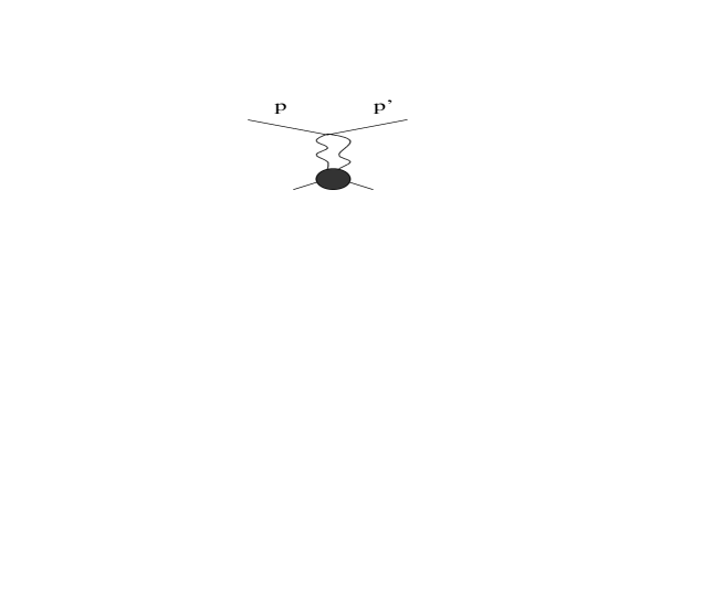
Figure 3: Diagram contributing to the Born Approximation

The interaction in question is shown in figure (3). Since the scattering of the CNF is with a colorless state the gluons are off-shell. What is said in effect is that the two gluons emerging from the upper vertex (fig. (3)) may split independently to form ‘fan’ diagrams [2], but will eventually form a colorless state. Further, since the interaction is a soft one, it can be assumed that the initial and final energy of the CNF is approximately equal, and the gluons posses the same momentum (flowing in opposite directions) given by:

$$k_{1}=-k_{2}=\frac{p-p^{\prime}}{2}.$$ (23)

With these approximations the amplitude can be given by the following:

$$<p^{\prime}|iT|p>=iV_{ab}^{ij}(k)M_{abij},$$ (24)

where

$$V^{ij}_{ab}=\lambda\delta_{ab}\frac{{\mathbf{k}}^{i}{\mathbf{k}}^{j}+\delta^{ij}|{\mathbf{k}}|^{2}}{|{\mathbf{k}}|^{4}},$$ (25)

and ${\mathbf{k}}=\frac{{\mathbf{p}}^{\prime}-{\mathbf{p}}}{2}$.

The term $M_{abij}$ is the amplitude arising from colorless states appearing on the bottom of the diagram (fig. 3) which in our approximation are independent of ${\mathbf{k}}$ and consist of higher order terms in QCD. In effect $V^{ij}_{ab}(k)$ is the potential arising from a process where a color neutral field interacts with a digluon colorless state.

Taking its Fourier transform the following is obtained:

$$V^{ij}_{ab}(x)=-\lambda\delta_{ab}\left(\nabla^{2}+\partial^{i}\partial^{j}\right)\int\frac{d^{3}{\mathbf{k}}}{(2\pi)^{3}}\frac{e^{i{\mathbf{k}}\cdot{\mathbf{x}}}}{|{\mathbf{k}}|^{4}}$$

$$=\lambda\delta_{ab}\frac{1}{3\pi r}\left(\delta^{ij}-\frac{1}{8r^{2}}Q^{ij}\right),$$ (26)

$Q^{ij}=3x^{i}x^{j}-\delta^{ij}r^{2}$.

The potential $V^{ij}_{ab}$ has split into two components; a monopole term, and a quadrupole term. This splitting has significance in the context of excited states of nucleons, or what are known as Regge trajectories. It is observed [16, 17] that in a $J/m^{2}$ plot there are transitions of angular momentum $\triangle J=2,0$ between hadronic states. In addition, there are algebraic models [5, 18] which utilize symmetries of hadronic states requiring volume conservation ($SL(3R)$, $SL(4R)$ spectrum generating algebras derived from confinement) that give such selection rules for these hadronic excitations. Such selection rules are derived from hadronic currents that are related to a ”shear” tensor, and a ”dilaton” scalar given by:

$$T^{\mu\nu} = \int d^{3}x\hskip 2.84544ptx^{\mu}\theta^{0\nu}+x^{\nu}\theta^{0\mu}-\frac{1}{4}g^{\mu\nu}x^{\sigma}\theta_{0\sigma}$$ (27)

$$D = \frac{1}{4}\int d^{3}x\hskip 2.84544ptx^{\sigma}\theta_{0\sigma},$$ (28)

where $\theta^{\nu\mu}$ is the energy momentum tensor for hadronic fields derived from QCD [5].

The shear tensor $T^{\mu\nu}$ is a traceless symmetric tensor. It contains a tensor $T^{ij}$ which transforms as a spherical tensor of rank two under rotations, and therefore has a non-zero expectation value between the states

$$<J|T^{ij}|J\pm 2>\neq 0.$$

This tensor provides excitations along a specific regge trajectory which stems from hadronic structure deformation with volume conservation. Thus it should couple to the quadrupole term in (26).

The tensor $D$ is a dilaton which transforms as a scalar under rotations, and therefore has a non-zero expectation value between states of the same angular momentum namely:

$$<J|D|J>\neq 0.$$

This tensor describes dilatations of hadronic fields, and therefore provides transitions between different regge trajectories; no volume conservation. Therefore it will couple to the monopole term in (26).

It is important to note that this potential can also arise for a field strength of an abelian gauge theory (electromagnetic field) coupled to a CNF. However following the discussion in section  (2), amplitudes in this model are proportional to $A\sim\left(\frac{q}{\Lambda}\right)^{d}$. This means that in the regge region a QED process will be suppressed by $\Lambda_{QED}$ which is much greater than $q$, and therefore will give terms that vanish. For QCD, $q$ and $\Lambda_{QCD}$ may be of the same order (in the IR region) producing a non-vanishing amplitude.

5 Conclusion

The use of the field strength in the IR region as a field theoretical tool to explain phenomena at low $q$ has already been utilized in other models especially concerning that of the Pomeron [3]. In this non-perturbative model Kharzeev and Levin have shown that the trace of the field strength (2) is directly proportional to the trace of the QCD energy momentum tensor which at small momentum (and assuming chiral symmetry), is proportional to the pion field and its momentum. Thus at long distances the two emerging gluons (by which the CNFs’ interact) hadronize to produce a pion in a first order approximation; a non-local process which is a direct result of the field strength interaction. Further, at low momenta it is believed that QCD gluon fields may be described by instantons. In obtaining these semi-classical solutions for the field equations [19], one defines a four volume on which $F^{\mu\nu}_{ab}$ is defined. Boundary conditions are then imposed on the three surface for the field strength rather than for the gauge field. It follows that in this scheme the field strength is taken to be a non-local object which effectively describes the semi-classical fluctuations of the gauge fields. All these models coincide with the picture that at low momentum the parton’s wave function becomes more spread and less localized due to the rise of the strong coupling. Since our model deals with color-neutral fields defined to be as non-local entities as a priori, it is only natural that some form of the field strength should play a role in describing interactions among these fields. Although our model is similar to the schemes mentioned above by the inclusion of the field strength at low energies, it differs from them in that the treatment here was perturbative, and thus may provide a bridge between the perturbative and the non-perturbative sectors of QCD.

References

- [1] S. Coleman, D. J. Gross, Phys. Rev. Lett. Lett. 31(1973)851.
- [2] L. V. Gribov, E. M. Levin, M. G. Ryskin, Physics Reports. 100(1983)1.
- [3] D. Kharzeev, E. M. Levin, Nucl. Phys. B. 578(2000)351.
- [4] E. A. Kuraev, L. N. Lipatov, V. S. Fadin, Sov. Phys. JETP 45(1977)199.
- [5] Y. Ne’eman, Dj. Sijacki, Phys. Rev. D. 37(1988)3267.
- [6] J. R. Forshaw and D. A.Ross, Quantum Chromodynamics and the Pomeron, Cambridge University Press, 1997.
- [7] P. D. B. Collins, Introduction to Regge Theory and High Energy Physics, Cambridge University Press, 1977.
- [8] M. E. Peskin, D. V. Schroeder, Introduction to Quatum Field Theory, Addison-Wesley Publishing Company, 1995, pp. 399-403.
- [9] R. E. Cutkosky, J. Math. Phys. 1(1960)429.
- [10] L. V. Gribov, Nucl. Phys. B. 168(1980)429.
- [11] D. J Gross, F. Wilczek, Phys. Rev. D. 9(1974)980.
- [12] Yu. L. Dokshitzer, ZhETF. 73(1977)1216.
- [13] V. F. Fadin, E. A. Kuraev, L. N. Lipatov. Phys. Lett. 60B(1975)150.
- [14] E. A. Kuraev, L. N. Lipatov, V. S. Fadin, Sov. Phys. JETP. 44(1976)443.
- [15] E. A. Kuraev, L. N. Lipatov, V. F. Fadin, ZhETF 72(1977)298.
- [16] A. V. Barnes et al, Phys. Rev. Lett. 37(1976)79.
- [17] G. F. P. Chew, S. C. Frautschi, Phys. Rev. Lett. 7(1961)394.
- [18] Y. Ne’eman Ann. Inst. Henry Poincare’. 28(1978)369.
- [19] L. H. Ryder, Quantum Field Theory, Cambridge University Press 1996, pp. 441-420.