KEK-TH-798 VPI-IPPAP-01-03 hep-ph/0112338 December, 2001

Prospects of Very Long Base-Line Neutrino Oscillation Experiments with the KEK-JAERI High Intensity Proton Accelerator

M. Aoki¹, K. Hagiwara¹, Y. Hayato², T. Kobayashi²,

T. Nakaya³, K. Nishikawa³, and N. Okamura⁴

¹Theory Group, KEK, Tsukuba, Ibaraki 305-0801, Japan
²Inst. of Particle and Nuclear Studies, High Energy Accelerator Research Org. (KEK), Tsukuba, Ibaraki 305-0801, Japan
³Department of Physics, Kyoto University, Kyoto 606-8502, Japan
⁴IPPAP, Physics Department, Virginia Tech. Blacksburg, VA 24061, USA

We study physics potential of Very Long Base-Line (VLBL) Neutrino-Oscillation Experiments with the High Intensity Proton Accelerator (HIPA), which will be completed by the year 2007 in Tokai-village, Japan, as a joint project of KEK and JAERI (Japan Atomic Energy Research Institute). The HIPA 50 GeV proton beam will deliver neutrino beams of a few GeV range with the intensity about two orders of magnitude higher than the present KEK beam for K2K experiment. As a sequel to the proposed HIPA-to-Super-Kamiokande experiment, we study impacts of experiments with a 100 kton-level detector and the base-line length of a few-thousand km. The pulsed narrow-band $\nu_{\mu}$ beams (NBB) allow us to measure the $\nu_{\mu}\to\nu_{e}$ transition probability and the $\nu_{\mu}$ survival probability through counting experiments at large water-$\check{\rm C}$erenkov detector. We study sensitivity of such experiments to the neutrino mass hierarchy, the mass-squared differences, the three angles, and one CP phase of the three-generation lepton-flavor-mixing matrix. We find that experiments at a distance between 1,000 and 2,000 km can determine the sign of the larger mass-squared difference $(m_{3}^{2}-m_{1}^{2})$ if the mixing between $\nu_{e}$ and $\nu_{3}$ (the heaviest-or-lightest neutrino) is not too small; $2|U_{e3}|^{2}(1-|U_{e3}|^{2})~{}{\hbox to0.0pt{\lower 3.5pt\hbox{$\mathchar 0\relax\sim$}\hss}\raise 1.0pt\hbox{$>$}}\,0.03$. The CP phase can be constrained if the $|U_{e3}|$ element is sufficiently large, $2|U_{e3}|^{2}(1-|U_{e3}|^{2})~{}{\hbox to0.0pt{\lower 3.5pt\hbox{$\mathchar 0\relax\sim$}\hss}\raise 1.0pt\hbox{$>$}}\,0.06$, and if the smaller mass-squared difference $(m_{2}^{2}-m_{1}^{2})$ and the $U_{e2}$ element are in the prefered range of the large-mixing-angle solution of the solar-neutrino deficit. The magunitude $\left|m_{3}^{2}-m_{1}^{2}\right|$ and the matrix element $U_{\mu 3}$ can be precisely measured, but we find little sensitivity to $m_{2}^{2}-m_{1}^{2}$ and the matrix element $U_{e2}$.

PACS : 14.60.Lm, 14.60.Pq, 01.50.My

Keywords: neutrino oscillation experiment, long base line experiments, future plan

1 Introduction

Many neutrino experiments [1]-[10] strongly suggest that there are flavor mixings in the lepton sector, and that neutrinos are massive. According to the atmospheric-neutrino observations [1], the lepton-flavor-mixing matrix (the Maki-Nakagawa-Sakata (MNS) matrix [11]) has a large mixing angle. Especially, the Super-Kamiokande (SK) collaboration [2] reported that $\nu_{\mu}$ oscillates into the other species with maximal mixing. The K2K [3] experiment, the current long-base-line (LBL) neutrino oscillation experiment from KEK to SK with $L=250$ km and $\langle E_{\nu}\rangle=1.3$ GeV, obtained results which are consistent with the neutrino oscillation in the atmospheric-neutrino anomaly with $\delta m^{2}\sim 3\times 10^{-3}$ and $\sin^{2}2\theta\sim 1$. The two reactor neutrino experiments CHOOZ [4] and Palo Verde [5] reported that no oscillation is found from $\overline{\nu}_{e}$, and they exclude significant mixings between $\overline{\nu}_{e}$ and the other neutrinos. An important conclusion from these observations is that the atmospheric neutrino oscillation cannot be due to $\nu_{\mu}$-$\nu_{e}$ oscillation. Recently, the SK collaboration showed an evidence that $\nu_{\mu}$ oscillates into an active neutrino rather than sterile neutrinos [6]. According to the results of solar-neutrino observations [7], the $\nu_{e}$ flux from the sun is less than that of the prediction of the standard solar model [8] and the reduction factor depends on neutrino energies. The most convincing explanation for this deficit is the $\nu_{e}$ oscillation to the other neutrinos. Four possible scenarios of the solar-neutrino oscillation have been identified : the MSW [12, 13] large-mixing-angle (LMA) solution, the MSW small-mixing-angle (SMA) solution, the vacuum oscillation (VO) solution [14] and the MSW low-$\delta m^{2}$ (LOW) solution. Recently, the SK collaboration reported the energy spectrum and the day-night asymmetry data and showed that the LMA solution is more favorable than the other scenarios [9]. The SNO experiment [10], which observes the solar neutrino flux with heavy water, showed conclusively, when combined with the SK flux data, that $\nu_{e}$ oscillates into the other active neutrinos [10]. A consistent picture of three-neutrino oscillations with two large mixing angles and two hierarchically different mass-squared differences emerges from those observations, with the exception of the LSND experiment [15] which may indicate the existence of the fourth and non-standard (sterile) neutrino.

Several LBL neutrino oscillation experiments [16, 17, 18, 19] and a short-base-line experiment [20] have been proposed to confirm the results of these experiments and to measure the neutrino oscillation parameters more precisely. The MINOS experiments [16], from Fermilab to the Soudan mine, with the base-line length of $L=730$ km and $\langle E_{\nu}\rangle=3.5$ GeV, will start producing data in 2005. The observation of the survival probability $P_{\nu_{\mu}\to\nu_{\mu}}$ will allow us to measure the larger mass-squared difference and the mixing angle with about $10\%$ accuracy. Two LBL experiments, ICARUS [17] and OPERA [18], from CERN to Gran-Sasso with the base-line length of $L=730$ km and at higher energies with $\langle E_{\nu}\rangle\sim 20$ GeV have been proposed, and they may begin operation in 2005. The CERN experiments expect to observe the $\nu_{\mu}\to\nu_{\tau}$ appearance. Physics discover potential of these LBL experiments have been studied extensively [21].

In Japan, as a sequel to the K2K experiment, a new LBL neutrino oscillation experiment between the High Intensity Proton Accelerator (HIPA) [22] and SK has been proposed [19]. The facility, HIPA, has a 50 GeV proton accelerator, which will be completed by the year 2007 in the site of JAERI (Japan Atomic Energy Research Institute), as the joint project of KEK and JAERI. The proton beam of HIPA can deliver high intensity neutrino beams in the $\sim 1$ GeV range, whose intensity is two-orders-of-magnitude higher than that of the KEK 12 GeV proton synchrotron beam for the K2K experiment. The HIPA-to-SK experiment with $L=295$ km and $\langle E_{\nu}\rangle=1.3$ GeV will measure the larger mass-squared difference with 3 $\%$ accuracy and the mixing angle at about 1 $\%$ accuracy.

All these experiments use conventional neutrino beams, which are made from decaying pions and Kaons that are produced by high-energy proton beams. The possibility of a neutrino factory [23] has been discussed as the next generation of LBL neutrino-oscillation experiments [24]. Here the neutrino beam is delivered from decaying muons in a muon-storage ring, where the stored muon energy may be in the several 10 GeV range. A neutrino factory can deliver very high intensity neutrino beams that are consist of the same amount of $\nu_{\mu}$ and $\overline{\nu}_{e}$ ($\overline{\nu}_{\mu}$ and $\nu_{e}$ from $\mu^{+}$) with precisely known spectra. Possibility of constructing a neutrino factory in the JAERI site by upgrading the HIPA is now being extensively studied [25].

In this paper we examine an alternative possibility of using conventional neutrino beams from the HIPA for Very-Long-Base-Line (VLBL) neutrino oscillation experiments, whose base-line length exceeding a thousand km [26]. A possible 100 kton detector in Beijing [27] can be a target at about $L=2,100$ km away. Physics capability of such experiments should be seriously studied because a neutrino factory may turn out to be too difficult or too expensive to realize in the near future. In order to take full advantage of conventional $\nu$ beams, we examine the case of using pulsed narrow-band $\nu_{\mu}$ beams (NBB) and as a target we consider a large water-$\check{\rm C}$erenkov detector a la SK which is capable of measuring the $\nu_{\mu}$-to-$\nu_{e}$ transition probability and the $\nu_{\mu}$ survival probability. We study sensitivity of such experiments to the signs and the magnitudes of the two mass-squared differences, the three angles and one CP phase of the three-flavor MNS matrix.

This article is organized as follows. In section 2, we fix our notation and review the present status of the neutrino-oscillation experiments in the three-neutrino model. In section 3, we study the properties of the narrow-band neutrino beams that can be delivered by the HIPA 50 GeV proton synchrotron. In section 4, we study the signals, the backgrounds and systematic errors of the VLBL experiments and present our findings for the prospects of experiments at the base-line length of 2,100 km and 1,200 km. Our results are summarized in section 5.

2 Neutrino oscillation in the three-neutrino model

In this section, we give the definition and useful parameterization of the 3$\times$3 Maki-Nakagawa-Sakata (MNS) lepton-flavor-mixing matrix [11], and give constraints on its matrix elements and the neutrino mass-squared differences.

2.1 The MNS matrix

The MNS matrix is defined analogously to the CKM matrix [28] through the charged-current (CC) weak interactions, where the charged-current can be expressed as

$$J^{\mu}_{\rm cc}=(\overline{d},\overline{s},\overline{b}){V_{{}_{\rm CKM}}^{\dagger}}\gamma^{\mu}(1-\gamma_{5})(u,c,t)^{T}+(\overline{e},\overline{\mu},\overline{\tau})\gamma^{\mu}(1-\gamma_{5}){V_{{}_{\rm MNS}}}(\nu_{1},\nu_{2},\nu_{3})^{T}\,.$$ (2.1)

Here $\nu_{i}~{}(i=1,2,3)$ denotes the neutrino mass-eigenstates. The flavor-eigenstates of the neutrinos are then expressed as

$$\nu_{\alpha}=\sum_{i=1}^{3}\left({{V}_{{}_{\rm MNS}}}\right)_{{\alpha}{i}}~{}{\nu_{i}}\,,$$ (2.2)

where $\alpha=e,\mu,\tau$ are the lepton-flavor indices.

The $3\times 3$ MNS matrix has three mixing angles and three phases in general. We adopt the following parameterization [29]

$$V_{{}_{\rm MNS}}=\left(\begin{array}[]{ccc}U_{e1}&U_{e2}&U_{e3}\\ U_{\mu 1}&U_{\mu 2}&U_{\mu 3}\\ U_{\tau 1}&U_{\tau 2}&U_{\tau 3}\end{array}\right)\left(\begin{array}[]{ccc}1&0&0\\ 0&e^{i\varphi_{2}}&0\\ 0&0&e^{i\varphi_{3}}\end{array}\right)\equiv U{\cal P}\,,$$ (2.3)

where ${\cal P}$ is the diagonal phase matrix with two Majorana phases, $\varphi_{2}$ and $\varphi_{3}$. The matrix $U$, which has three mixing angles and one phase, can be parameterized in the same way as the CKM matrix. Because the present neutrino oscillation experiments constrain directly the elements, $U_{e2}$, $U_{e3}$, and $U_{\mu 3}$, we find it most convenient to adopt the parameterization [29] where these three matrix elements in the upper-right corner of the $U$ matrix are the independent parameters. Without losing generality, we can take $U_{e2}$ and $U_{\mu 3}$ to be real and non-negative. By allowing $U_{e3}$ to have the complex phase

$$U_{e2},U_{\mu 3}\geq 0,~{}~{}~{}U_{e3}\equiv\left|U_{e3}\right|e^{-i\delta_{{}_{\rm MNS}}}~{}~{}(0\leq\delta_{{}_{\rm MNS}}<2\pi)\,,$$ (2.4)

the four independent parameters are $U_{e2},U_{\mu 3},|U_{e3}|$ and $\delta_{{}_{\rm MNS}}$. All the other matrix elements of the $U$ are then determined by the unitary conditions :

$$U_{e1} = \sqrt{1-|U_{e3}|^{2}-|U_{e2}|^{2}}\,,~{}~{}~{}~{}~{}U_{\tau 3}=\sqrt{1-|U_{e3}|^{2}-|U_{\mu 3}|^{2}}\,,$$ (2.5a)

$$U_{\mu 1} = -\frac{U_{e2}U_{\tau 3}+U_{\mu 3}U_{e1}U_{e3}^{\ast}}{1-|U_{e3}|^{2}}\,,~{}~{}U_{\mu 2}=\frac{U_{e1}U_{\tau 3}-U_{\mu 3}U_{e2}U_{e3}^{\ast}}{1-|U_{e3}|^{2}}\,,$$ (2.5b)

$$U_{\tau 1} = \frac{U_{e2}U_{\mu 3}-U_{\tau 3}U_{e1}U_{e3}^{\ast}}{1-|U_{e3}|^{2}}\,,~{}~{}~{}~{}U_{\tau 2}=-\frac{U_{\mu 3}U_{e1}+U_{e2}U_{\tau 3}U_{e3}^{\ast}}{1-|U_{e3}|^{2}}\,.$$ (2.5c)

In this phase convention, $U_{e1}$, $U_{e2}$, $U_{\mu 3}$, and $U_{\tau 3}$ are all real and non-negative numbers, and the other five elements are complex numbers.

The Jarlskog parameter [30] of the MNS matrix is defined as

$$J_{{}_{\rm MNS}}\equiv{\rm Im}\left({V_{\alpha i}V_{\beta i}^{\ast}V_{\beta j}V_{\alpha j}^{\ast}}\right)={\rm Im}\left({U_{\alpha i}U_{\beta i}^{\ast}U_{\beta j}U_{\alpha j}^{\ast}}\right)=-\frac{U_{e1}U_{e2}U_{\mu 3}U_{\tau 3}}{1-\left|U_{e3}\right|^{2}}{\rm Im}\left({U_{e3}}\right)\,,$$ (2.6)

where $(\alpha,\beta)=(e,\mu),(\mu,\tau),(\tau,e)$ and $(i,j)=(1,2),(2,3),(3,1)$. The last expression above is obtained in our phase convention. The two Majorana phases $\varphi_{2}$ and $\varphi_{3}$ do not contribute to the Jarlskog parameter.

2.2 Constraints on the MNS matrix and the mass-squared differences

The probability of finding the flavor-eigenstate $\beta$ from the original flavor-eigenstate $\alpha$ at the base-line length $L$ in the vacuum is given by

$$P_{\nu_{\alpha}\to\nu_{\beta}} = \left|\sum_{j=1}^{3}(V_{{}_{\rm MNS}})_{\beta j}\exp\left(-i\frac{m_{j}^{2}}{2E_{\nu}}L\right)(V_{{}_{\rm MNS}})_{j\alpha}\right|^{2}$$ (2.7)

$$= \left|U_{\beta 1}U_{\alpha 1}^{\ast}+U_{\beta 2}e^{-i\Delta_{12}}U_{\alpha 2}^{\ast}+U_{\beta 3}e^{-i\Delta_{13}}U_{\alpha 3}^{\ast}\right|^{2}$$

$$= \delta_{\alpha\beta}-4{\rm Re}\left\{U_{\alpha 1}U_{\beta 1}^{\ast}U_{\beta 2}U_{\alpha 2}^{\ast}\sin^{2}\frac{\Delta_{12}}{2}+U_{\alpha 2}U_{\beta 2}^{\ast}U_{\beta 3}U_{\alpha 3}^{\ast}\sin^{2}\frac{\Delta_{23}}{2}+U_{\alpha 3}U_{\beta 3}^{\ast}U_{\beta 1}U_{\alpha 1}^{\ast}\sin^{2}\frac{\Delta_{31}}{2}\right\}$$

$$~{}~{}~{}~{}~{}~{}+2{\rm Im}\left[U_{\alpha 1}U_{\beta 1}^{\ast}U_{\beta 2}U_{\alpha 2}^{\ast}\right]\left[\sin\Delta_{12}+\sin\Delta_{23}+\sin\Delta_{31}\right],$$

where $\Delta_{ij}$ is

$$\Delta_{ij}\equiv\frac{\delta m_{ij}^{2}}{2E_{\nu}}L\simeq 2.534\frac{\delta m_{ij}^{2}({\rm eV}^{2})}{E_{\nu}({\rm GeV})}L({\rm km})\,,$$ (2.8)

with the neutrino energy $E_{\nu}$ and the mass-squared differences $\delta m_{ij}^{2}=m_{j}^{2}-m_{i}^{2}$. In particular, the survival probability in the vacuum is

$$P_{\nu_{\alpha}\to\nu_{\alpha}} = 1-4\left\{\left|U_{\alpha 1}U_{\alpha 2}\right|^{2}\sin^{2}\frac{\Delta_{12}}{2}+\left|U_{\alpha 2}U_{\alpha 3}\right|^{2}\sin^{2}\frac{\Delta_{23}}{2}+\left|U_{\alpha 3}U_{\alpha 1}\right|^{2}\sin^{2}\frac{\Delta_{31}}{2}\right\}\,.$$ (2.9)

The oscillation probabilities of anti-neutrinos in the vacuum are obtained from those of neutrinos simply by reversing the sign of the Jarlskog parameter;

$$P_{\overline{\nu}_{\alpha}\to\overline{\nu}_{\alpha}} = P_{\nu_{\alpha}\to\nu_{\alpha}}\,,$$ (2.10a)

$$P_{\overline{\nu}_{\alpha}\to\overline{\nu}_{\beta}} = P_{\nu_{\alpha}\to\nu_{\beta}}(J_{{}_{\rm MNS}}\to-J_{{}_{\rm MNS}})\,.$$ (2.10b)

For instance,

$$\left(\begin{array}[]{c}P_{\nu_{\mu}\to\nu_{e}}\\ P_{\overline{\nu}_{\mu}\to\overline{\nu}_{e}}\end{array}\right) = -4{\rm Re}\left\{U_{\mu 1}U_{e1}^{\ast}U_{e2}U_{\mu 2}^{\ast}\sin^{2}\frac{\Delta_{12}}{2}+U_{\mu 2}U_{e2}^{\ast}U_{e3}U_{\mu 3}^{\ast}\sin^{2}\frac{\Delta_{23}}{2}\right.$$ (2.14)

$$+\left.U_{\mu 3}U_{e3}^{\ast}U_{e1}U_{\mu 1}^{\ast}\sin^{2}\frac{\Delta_{31}}{2}\right\}\mp 2J_{{}_{\rm MNS}}\left\{\sin\Delta_{12}+\sin\Delta_{23}+\sin\Delta_{31}\right\}\,.~{}~{}~{}~{}~{}$$

The unitarity leads to the identities

$$\sum_{\beta=e,\mu,\tau}P_{\nu_{\alpha}\to\nu_{\beta}}=\sum_{\beta=e,\mu,\tau}P_{\nu_{\beta}\to\nu_{\alpha}}=\sum_{\beta=e,\mu,\tau}P_{\overline{\nu}_{\alpha}\to\overline{\nu}_{\beta}}=\sum_{\beta=e,\mu,\tau}P_{\overline{\nu}_{\beta}\to\overline{\nu}_{\alpha}}=1\,.$$ (2.15)

The following approximations for the oscillation probabilities are useful in our study. When $\left|\Delta_{12}\right|\ll\left|\Delta_{13}\right|\sim 1$, the oscillation probabilities can be expressed as

$$P_{\nu_{\alpha}\to\nu_{\beta}} = \delta_{\alpha\beta}-4{\rm Re}\left\{U_{\alpha 3}U_{\beta 3}^{\ast}U_{\beta 1}U_{\alpha 1}^{\ast}+U_{\alpha 2}U_{\beta 2}^{\ast}U_{\beta 3}U_{\alpha 3}^{\ast}\right\}\sin^{2}\displaystyle\frac{\Delta_{13}}{2}$$ (2.16)

$$+\left\{2{\rm Re}\left(U_{\alpha 2}U_{\beta 2}^{\ast}U_{\beta 3}U_{\alpha 3}^{\ast}\right)\sin\Delta_{13}\pm 4J_{\rm MNS}\sin^{2}\displaystyle\frac{\Delta_{13}}{2}\right\}\Delta_{12}$$

$$+{\rm Re}\left(U_{\alpha 1}U_{\beta 1}^{\ast}U_{\beta 2}U_{\alpha 2}^{\ast}+U_{\alpha 2}U_{\beta 2}^{\ast}U_{\beta 3}U_{\alpha 3}^{\ast}\cos\Delta_{13}\right)\Delta_{12}^{2}+{\cal O}(\Delta_{12}^{3})\,.$$

When $1\ll\left|\Delta_{12}\right|\sim\left|\Delta_{13}\right|$, we may take into account finite resolution of $\Delta_{ij}$ $(\Delta_{ij}\to\Delta_{ij}\pm\delta\Delta_{ij})$, and find

$$P_{\nu_{\alpha}\to\nu_{\beta}} \to \displaystyle\frac{1}{2\delta\Delta_{ij}}\int_{{}_{\Delta_{ij}-\delta\Delta_{ij}}}^{{}^{\Delta_{ij}+\delta\Delta_{ij}}}d\Delta_{ij}P_{\nu_{\alpha}\to\nu_{\beta}}\left(\Delta_{ij}\right)$$ (2.17)

$$= \delta_{\alpha\beta}-2{\rm Re}\left\{U_{\alpha 1}U_{\beta 1}^{\ast}U_{\beta 2}U_{\alpha 2}^{\ast}+U_{\alpha 2}U_{\beta 2}^{\ast}U_{\beta 3}U_{\alpha 3}^{\ast}+U_{\alpha 3}U_{\beta 3}^{\ast}U_{\beta 1}U_{\alpha 1}^{\ast}\right\}$$

$$+2{\rm Re}\left\{U_{\alpha 1}U_{\beta 1}^{\ast}U_{\beta 2}U_{\alpha 2}^{\ast}\cos{\Delta_{12}}\displaystyle\frac{\sin{\delta\Delta_{12}}}{\delta\Delta_{12}}+U_{\alpha 2}U_{\beta 2}^{\ast}U_{\beta 3}U_{\alpha 3}^{\ast}\cos{\Delta_{23}}\displaystyle\frac{\sin{\delta\Delta_{23}}}{\delta\Delta_{23}}\right.$$

$$~{}~{}~{}~{}~{}~{}~{}~{}~{}~{}\left.+U_{\alpha 3}U_{\beta 3}^{\ast}U_{\beta 1}U_{\alpha 1}^{\ast}\cos{\Delta_{31}}\displaystyle\frac{\sin{\delta\Delta_{31}}}{\delta\Delta_{31}}\right\}$$

$$\pm 2J_{{}_{\rm MNS}}\left\{\sin{\Delta_{12}}\displaystyle\frac{\sin{\delta\Delta_{12}}}{\delta\Delta_{12}}+\sin{\Delta_{23}}\displaystyle\frac{\sin{\delta\Delta_{23}}}{\delta\Delta_{23}}+\sin{\Delta_{31}}\displaystyle\frac{\sin{\delta\Delta_{31}}}{\delta\Delta_{31}}\right\}\,.$$

In LBL experiments the uncertainty in $E_{\nu}$, $\delta E_{\nu}$, dictates $\Delta_{ij}$,

$$\delta\Delta_{ij}\simeq-\Delta_{ij}\displaystyle\frac{\delta E_{\nu}}{E_{\nu}}\,,$$ (2.18)

and the following two cases are relevant. When

$$\left|\delta\Delta_{12}\right|\simeq\left|\Delta_{12}\displaystyle\frac{\delta E_{\nu}}{E_{\nu}}\right|\ll 1\ll\left|\Delta_{13}\displaystyle\frac{\delta E_{\nu}}{E_{\nu}}\right|\simeq\left|\delta\Delta_{13}\right|\simeq\left|\delta\Delta_{23}\right|\,,$$ (2.19)

eq.(2.17) can be expressed as

$$P_{\nu_{\alpha}\to\nu_{\beta}}\to\delta_{\alpha\beta} - 2{\rm Re}\left\{U_{\alpha 1}U_{\beta 1}^{\ast}U_{\beta 2}U_{\alpha 2}^{\ast}+U_{\alpha 2}U_{\beta 2}^{\ast}U_{\beta 3}U_{\alpha 3}^{\ast}+U_{\alpha 3}U_{\beta 3}^{\ast}U_{\beta 1}U_{\alpha 1}^{\ast}\right\}$$ (2.20)

$$+2{\rm Re}\left\{U_{\alpha 1}U_{\beta 1}^{\ast}U_{\beta 2}U_{\alpha 2}^{\ast}\cos{\Delta_{12}}\right\}\pm 2J_{{}_{\rm MNS}}\left\{\sin{\Delta_{12}}\right\}$$

$$+{\cal O}\left(\left(\Delta_{12}\displaystyle\frac{\delta E_{\nu}}{E_{\nu}}\right)^{2}\right)+{\cal O}\left(\left(\Delta_{13}\displaystyle\frac{\delta E_{\nu}}{E_{\nu}}\right)^{-1}\right)\,.$$

On the other hand, when

$$1\ll\left|\Delta_{12}\displaystyle\frac{\delta E_{\nu}}{E_{\nu}}\right|\ll\left|\Delta_{13}\displaystyle\frac{\delta E_{\nu}}{E_{\nu}}\right|$$ (2.21)

eq.(2.17) is simplified to

$$P_{\nu_{\alpha}\to\nu_{\beta}}\to\delta_{\alpha\beta} - 2{\rm Re}\left\{U_{\alpha 1}U_{\beta 1}^{\ast}U_{\beta 2}U_{\alpha 2}^{\ast}+U_{\alpha 2}U_{\beta 2}^{\ast}U_{\beta 3}U_{\alpha 3}^{\ast}+U_{\alpha 3}U_{\beta 3}^{\ast}U_{\beta 1}U_{\alpha 1}^{\ast}\right\}$$ (2.22)

$$+{\cal O}\left(\left(\Delta_{12}\displaystyle\frac{\delta E_{\nu}}{E_{\nu}}\right)^{-1}\right)+{\cal O}\left(\left(\Delta_{13}\displaystyle\frac{\delta E_{\nu}}{E_{\nu}}\right)^{-1}\right)\,.$$

Note that in eqs.(2.16), (2.17), and (2.20), $\pm J_{{}_{\rm MNS}}$ stands for ${\rm Im}\left[U_{\alpha 1}U_{\beta 1}^{\ast}U_{\beta 2}U_{\alpha 2}^{\ast}\right]$; see eq.(2.6).

All the above formulas remain valid for the neutrino oscillation probabilities in the matter, by replacing the mass-squared differences and the MNS matrix elements with the effective ones in the matter,

$$\Delta_{ij}\to\widetilde{\Delta}_{ij}\,,~{}~{}U_{\alpha i}\to\widetilde{U}_{\alpha i}\,,~{}~{}J_{{}_{\rm MNS}}\to\widetilde{J}_{{}_{\rm MNS}}\,,$$ (2.23)

as long as the matter density remains the same along the base-line. The definitions of the effective parameters $\widetilde{\Delta}_{ij}$ and $\widetilde{U}_{\alpha i}$ are given in section 2.4,  and $\widetilde{J}_{{}_{\rm MNS}}$ is obtained from eq.(2.6) by replacing all $U_{\alpha i}$’s by $\widetilde{U}_{\alpha i}$’s.

In the following, we summarize the constraints on the neutrino mass-squared differences and the MNS matrix elements from the recent neutrino-oscillation experiments; the atmospheric-neutrino anomaly [1, 2], the CHOOZ reactor experiment [4], and the solar-neutrino deficit observations [7, 9, 10].

2.2.1 Atmospheric-neutrino anomaly

A recent analysis of the atmospheric-neutrino data from the Super-Kamiokande (SK) experiment [2] finds

$$0.88< \sin^{2}2\theta_{{}_{\rm ATM}} <1.0\,,$$ (2.24a)

$$1.6\times 10^{-3}< \delta m^{2}_{{}_{\rm ATM}}({\rm eV}^{2}) <4.0\times 10^{-3}\,,$$ (2.24b)

from the $\nu_{\mu}\to\nu_{\mu}$ survival probability in the two-flavor oscillation model:

$$P_{\nu_{\mu}\to\nu_{\mu}}=1-\sin^{2}2\theta_{{}_{\rm ATM}}\sin^{2}\left(\frac{\delta m^{2}_{{}_{\rm ATM}}}{4E_{\nu}}L\right).$$ (2.25)

The base-line of this observation is less than about $10^{4}$ km for the Earth diameter, and the typical neutrino energy is one to a few GeV. The survival probability eq.(2.9) may then be expanded as

$$P_{\nu_{\mu}\to\nu_{\mu}}=1-4\left|U_{\mu 3}\right|^{2}\left(1-\left|U_{\mu 3}\right|^{2}\right)\sin^{2}\frac{\Delta_{13}}{2}+2\left|U_{\mu 2}\right|^{2}\left|U_{\mu 3}\right|^{2}\Delta_{12}\sin\Delta_{13}+{\cal O}(\Delta_{12}^{2})\,.~{}~{}~{}~{}~{}~{}~{}$$ (2.26)

When $|\Delta_{12}|\ll 1$, we may neglect terms of order $\Delta_{12}$ and obtain the following identification :

$$4|U_{\mu 3}|^{2}(1-|U_{\mu 3}|^{2}) = \sin^{2}2\theta_{{}_{\rm ATM}}\,,$$ (2.27a)

$$\left|\delta m^{2}_{13}\right| = \delta m^{2}_{{}_{\rm ATM}}\,.$$ (2.27b)

The independent parameter $U_{\mu 3}$ ($\geq 0$ in our convention) is then

$$U_{\mu 3}=\sqrt{1-\sqrt{1-\sin^{2}2\theta_{{}_{\rm ATM}}}}\Bigg{/}\sqrt{2}\,.$$ (2.28)

The magnitude of the neglected terms in the above approximation is largest when the large-mixing-angle solution of the solar-neutrino deficit is taken. For $\delta m^{2}_{{}_{\rm SOL}}=10^{-4}$ eV², $E_{\nu}=1$ GeV, and $L=10^{4}$ km, we have $|\Delta_{12}|\simeq\delta m^{2}_{{}_{\rm SOL}}(L/2E_{\nu})\sim 1$, and a more careful analyses in the three-neutrino model are required to constrain the model parameters. The results of such analyses [31] show that the identifications eqs.(2.2.1) remain valid approximately even for the large-mixing-angle solution.

2.2.2 Reactor neutrino experiments

The CHOOZ experiment [4] measured the survival probability of $\overline{\nu}_{e}$,

$$P_{\overline{\nu}_{e}\to\overline{\nu}_{e}}=1-\sin^{2}2\theta_{{}_{\rm CHOOZ}}\sin^{2}\left(\frac{\delta m^{2}_{{}_{\rm CHOOZ}}}{4E_{\nu}}L\right)\,,$$ (2.29)

and it was found that

$$\sin^{2}2\theta_{{}_{\rm CHOOZ}}<\left\{\begin{array}[]{lcl}0.10{}{}&{\mbox{{ for }}}&\delta m^{2}_{{}_{\rm CHOOZ}}>3.5\times 10^{-3}\,{\rm eV}^{2}\,,\\ \\ 0.18{}{}&{\mbox{{ for }}}&\delta m^{2}_{{}_{\rm CHOOZ}}>2.0\times 10^{-3}\,{\rm eV}^{2}\,,\\ \\ 0.52{}{}&{\mbox{{ for }}}&\delta m^{2}_{{}_{\rm CHOOZ}}>1.0\times 10^{-3}\,{\rm eV}^{2}\,.\end{array}\right.$$ (2.35)

The base-line length of this experiment is about 1 km and the typical anti-neutrino energy is 1 MeV. For those $L$ and $E_{\nu}$, the Earth matter effects are negligible, and $|\Delta_{12}|=\delta m^{2}_{{}_{\rm SOL}}(L/2E_{\nu})$ can be safely neglected even for the large-mixing-angle solution. The survival probability of the three-neutrino model is then approximated by

$$P_{\overline{\nu}_{e}\to\overline{\nu}_{e}}=1-4\left|U_{e3}\right|^{2}\left(1-\left|U_{e3}\right|^{2}\right)\sin^{2}\displaystyle\frac{\Delta_{13}}{2}+{\cal O}(\Delta_{12})\,,$$ (2.36)

and we obtain the identifications :

$$4\left|U_{e3}\right|^{2}\left(1-\left|U_{e3}\right|^{2}\right) = \sin^{2}2\theta_{{}_{\rm CHOOZ}}\,,$$ (2.37a)

$$|\delta m^{2}_{13}| = \delta m^{2}_{{}_{\rm CHOOZ}}.$$ (2.37b)

With the above identifications, we find that the element $\left|U_{e3}\right|$ eq.(2.37a) is constrained by eq.(2.35) in the region of $|\delta m^{2}_{13}|$ allowed by the atmospheric-neutrino oscillation data through eq.(2.24b) and eq.(2.27b). The independent parameter $U_{e3}$ is now constrained by eq.(2.35) through the identification

$$\left|U_{e3}\right|=\sqrt{1-\sqrt{1-\sin^{2}2\theta_{{}_{\rm CHOOZ}}}}\Bigg{/}\sqrt{2}\,.$$ (2.38)

2.2.3 Solar-neutrino deficit

Deficit of the solar neutrinos observed at several terrestrial experiments [7, 9, 10] have been successfully interpreted in terms of the $\nu_{e}\to\nu_{X}$ ($\nu_{X}\neq\nu_{e}$ or $\overline{\nu}_{e}$) oscillation

$$P_{\nu_{e}\to\nu_{e}}=1-\sin^{2}2\theta_{{}_{\rm SOL}}\sin^{2}\left(\frac{\delta m^{2}_{{}_{\rm SOL}}}{4E_{\nu}}L\right)$$ (2.39)

in the following four scenarios [7, 9, 10].

MSW large-mixing-angle solution (LMA) :

$$0.7< \sin^{2}2\theta_{{}_{\rm SOL}} <0.9\,,$$ (2.40a)

$$3\times 10^{-5}< \delta m^{2}_{{}_{\rm SOL}}(\mbox{eV}^{2}) <15\times 10^{-5}\,.$$ (2.40b)

MSW small-mixing-angle solution (SMA) :

$$1.2\times 10^{-3}< \sin^{2}2\theta_{{}_{\rm SOL}} <12\times 10^{-3}\,,$$ (2.41a)

$$0.3\times 10^{-5}< \delta m^{2}_{{}_{\rm SOL}}(\mbox{eV}^{2}) <1\times 10^{-5}\,.$$ (2.41b)

MSW low-$\delta m^{2}$ solution (LOW) :

$$0.8< \sin^{2}2\theta_{{}_{\rm SOL}} \leq 1\,,$$ (2.42a)

$$10^{-8}< \delta m^{2}_{{}_{\rm SOL}}(\mbox{eV}^{2}) <2.5\times 10^{-7}\,.$$ (2.42b)

Vacuum Oscillation solution (VO) :

$$\sin^{2}2\theta_{{}_{\rm SOL}} \sim 0.9\,,$$ (2.43a)

$$\delta m^{2}_{{}_{\rm SOL}}(\mbox{eV}^{2}) \sim 10^{-9}\,.$$ (2.43b)

The SK collaboration reported that their data on the energy spectrum and the day-night asymmetry disfavor the SMA solution at $95\%$ C.L.. Recently the SNO collaboration gives us the first direct indication of a non-electron and active flavor component in the solar neutrino flux. Because $\delta m_{{}_{\rm ATM}}^{2}\gg\delta m_{{}_{\rm SOL}}^{2}$ the $\nu_{e}$ survival probability in the three-neutrino model can be expressed as

$$P_{\nu_{e}\to\nu_{e}}=1-2\left|U_{e3}\right|^{2}\left(1-\left|U_{e3}\right|^{2}\right)-4\left|U_{e1}\right|^{2}\left|U_{e2}\right|^{2}\sin^{2}\left(\displaystyle\frac{\Delta_{12}}{2}\right)+{\cal O}\left(\displaystyle\frac{E_{\nu}}{\delta E_{\nu}\Delta_{13}}\right)\,,$$ (2.44)

where terms of order $\left[\Delta_{13}\left(\delta E_{\nu}/E_{\nu}\right)\right]^{-1}$ in eq.(2.17) are safely neglected. The energy-independent deficit factor, $2|U_{e3}|^{2}(1-|U_{e3}|^{2})$, should be smaller than $5\%$ by the CHOOZ constraint eq.(2.35) if $\left|\delta m_{13}^{2}\right|>3.5\times 10^{-3}$eV². Because we need only rough estimates of the allowed ranges of the MNS matrix elements, we ignore the small energy-independent deficit factor and interpret the results of the two-flavor analysis eq.(2.40a)-eq.(2.43a) by using the following identifications

$$4\left|U_{e1}\right|^{2}\left|U_{e2}\right|^{2} = \sin^{2}2\theta_{{}_{\rm SOL}}\,,$$ (2.45a)

$$|\delta m^{2}_{12}| = \delta m^{2}_{{}_{\rm SOL}}\,.$$ (2.45b)

By using unitary condition, the independent parameter $U_{e2}$ is obtained as

$$U_{e2}=\left[\left(1-|U_{e3}|^{2}-\sqrt{\left(1-|U_{e3}|^{2}\right)^{2}-\sin^{2}2\theta_{{}_{\rm SOL}}}\right)\Bigg{/}2\right]^{1/2}\,.$$ (2.46)

2.3 Neutrino mass hierarchy

All the above constraints on the three-neutrino model parameters are obtained from the survival probabilities which are even-functions of $\delta m^{2}_{ij}$. We have made the identification

$$\delta m^{2}_{{}_{\rm SOL}}=\left|\delta m^{2}_{12}\right|\ll\left|\delta m^{2}_{13}\right|=\delta m^{2}_{{}_{\rm ATM}}\,,$$ (2.47)

which is valid for all the four scenarios of the solar neutrino oscillation.

There are four mass hierarchy cases corresponding to the sign of the $\delta m^{2}_{ij}$, as shown in Fig. 1 and Table 1. We name them the neutrino mass hierarchy I, II, III and IV, respectively.

	I	II	III	IV
$\delta m_{12}^{2^{\,}}$	$+\delta m_{\rm SOL}^{2}$	$-\delta m_{\rm SOL}^{2}$	$+\delta m_{\rm SOL}^{2}$	$-\delta m_{\rm SOL}^{2}$
$\delta m_{13}^{2^{\,}}$	$+\delta m_{\rm ATM}^{2}$	$+\delta m_{\rm ATM}^{2}$	$-\delta m_{\rm ATM}^{2}$	$-\delta m_{\rm ATM}^{2}$

Table 1: The four neutrino mass hierarchies and the corresponding sign assignments for $\delta m^{2}_{12}$ and $\delta m^{2}_{13}$.

If the MSW effect is relevant for the solar neutrino oscillation, then the neutrino mass hierarchy cases II and IV are not favored, especially for the LMA and SMA solutions. The hierarchy I may be called ‘normal’ and the hierarchy III may be called ‘inverted’. Within the three-neutrino model, there is an indication that the normal hierarchy I is favored against the inverted one III from the Super-Nova 1987A observation [33]. Nevertheless a terrestrial experiment is needed to determine the neutrino mass hierarchy.

Figure 1: Schematical view of the four-types of neutrino mass hierarchy.

We notice here that there are two types of mass eigenstate for the neutrinos. The states $\nu_{i}$ with the mass $m_{i}~{}(i=1,2,3)$ appear in the definition eq.(2.2) of the MNS matrix, whose elements are constrained by the existing experiments that measure essentially the neutrino-flavor survival probabilities. Since the survival probabilities eq.(2.9) do not depend on the sign of the mass-squared differences, these constraints do not depend on the neutrino mass hierarchy. Because the MNS matrix elements are constrained uniquely by the neutrino-flavor survival probabilities, we may call these states as ‘current-based’ mass-eigenstates. We find this basis most convenient for our study in this paper. On the other hand, the ‘mass-ordered’ mass-eigenstates $\nu^{\prime}_{i}$, whose masses satisfy

$$m^{\prime}_{1}<m^{\prime}_{2}<m^{\prime}_{3}\,,$$ (2.48)

are useful when studying the high-energy behavior of the neutrino mass matrix [34], the matter effects on the neutrino-flavor oscillation [12, 13], and when studying the lepton-number violation effects which are proportional to the magnitudes of the Majorana masses. The relation between the current-eigenstates and the two mass-eigenstates is

$$\left(\begin{array}[]{c}\nu_{e}\\ \nu_{\mu}\\ \nu_{\tau}\end{array}\right)=V_{{}_{\rm MNS}}\left(\begin{array}[]{c}\nu_{1}\\ \nu_{2}\\ \nu_{3}\end{array}\right)=V^{\prime}_{{}_{\rm MNS}}\left(\begin{array}[]{c}\nu^{\prime}_{1}\\ \nu^{\prime}_{2}\\ \nu^{\prime}_{3}\end{array}\right)\,,$$ (2.49)

where $V^{\prime}_{{}_{\rm MNS}}$ is the MNS matrix in the mass-ordered mass-eigenstate base. It can be obtained from $V_{{}_{\rm MNS}}$ by

$$V^{\prime}_{{}_{\rm MNS}}=V_{{}_{\rm MNS}}O^{\rm X}\mbox{{~{}~{}~{}~{}~{}(X = I, II, III, IV)}}\,,$$ (2.50)

where the permutation matrices $O^{\rm X}$

$$O^{\rm I}=\left(\begin{array}[]{ccc}1&0&0\\ 0&1&0\\ 0&0&1\end{array}\right)\,,O^{\rm II}=\left(\begin{array}[]{ccc}0&1&0\\ 1&0&0\\ 0&0&1\end{array}\right)\,,O^{\rm III}=\left(\begin{array}[]{ccc}0&1&0\\ 0&0&1\\ 1&0&0\end{array}\right),O^{\rm IV}=\left(\begin{array}[]{ccc}0&0&1\\ 0&1&0\\ 1&0&0\end{array}\right)\,~{}~{}~{}$$ (2.63)

relate the two mass-eigenstates

$$\left(\begin{array}[]{c}\nu_{1}\\ \nu_{2}\\ \nu_{3}\end{array}\right)=O^{\rm X}\left(\begin{array}[]{c}\nu^{\prime}_{1}\\ \nu^{\prime}_{2}\\ \nu^{\prime}_{3}\end{array}\right)\,,$$ (2.64)

for the neutrino mass hierarchy I, II, III and IV, respectively.

2.4 Neutrino oscillation in the Earth matter

Neutrino-flavor oscillation inside matter is governed by the Schrödinger equation

$$i\frac{\partial}{\partial t}\left(\begin{array}[]{c}\nu_{e}\\ \nu_{\mu}\\ \nu_{\tau}\\ \end{array}\right)=\frac{1}{2E_{\nu}}\left[{H_{0}}+\left(\begin{array}[]{ccc}a&0&0\\ 0&0&0\\ 0&0&0\end{array}\right)\right]\left(\begin{array}[]{c}\nu_{e}\\ \nu_{\mu}\\ \nu_{\tau}\\ \end{array}\right)=H\left(\begin{array}[]{c}\nu_{e}\\ \nu_{\mu}\\ \nu_{\tau}\\ \end{array}\right),$$ (2.77)

where $H_{0}$ is the Hamiltonian in the vacuum,

$$H_{0}={U}\left(\begin{array}[]{ccc}0&0&0\\ 0&\delta m^{2}_{21}&0\\ 0&0&\delta m^{2}_{31}\end{array}\right){U^{\dagger}}\,,$$ (2.81)

and $a$ is the matter effect term [12],

$$a=2\sqrt{2}G_{F}n_{e}E_{\nu}={7.56}\times 10^{-5}({\rm eV}^{2})\left(\frac{\rho}{{\rm g/cm}^{3}}\right)\left(\frac{E_{\nu}}{\rm GeV}\right)\,.$$ (2.82)

Here $n_{e}$ is the electron density of the matter, $G_{F}$ is the Fermi constant, and $\rho$ is the matter density. In our analysis, we assume that the density of the earth’s crust relevant for the VLBL experiments up to about 2,000 km is a constant, $\rho=3$, with an uncertainty of $\Delta\rho=0.1$;

$$\rho~{}({\rm g/cm}^{3})=3.0\pm 0.1\,.$$ (2.83)

The Hamiltonian in the matter $H$ is diagonalized as

$${H}=\displaystyle\frac{1}{2E_{\nu}}{{\widetilde{U}}}\left(\begin{array}[]{ccc}{\lambda_{1}}&0&0\\ 0&{\lambda_{2}}&0\\ 0&0&{\lambda_{3}}\end{array}\right){{\widetilde{U}^{\dagger}}},$$ (2.87)

by the MNS matrix in the matter $\widetilde{U}$. The neutrino-flavor oscillation probabilities in the matter

$$P_{\nu_{\alpha}\to\nu_{\beta}} = \left|\widetilde{U}_{\beta 1}\widetilde{U}_{\alpha 1}^{\ast}+\widetilde{U}_{\beta 2}e^{-i{{\widetilde{\Delta}_{12}}}}\widetilde{U}_{\alpha 2}^{\ast}+\widetilde{U}_{\beta 3}e^{-i{{\widetilde{\Delta}_{13}}}}\widetilde{U}_{\alpha 3}^{\ast}\right|^{2}\,$$ (2.88)

takes the same form as those in the vacuum eq.(2.7), where the elements $U_{\alpha i}$ are replaced by $\widetilde{U}_{\alpha i}$ and the terms $\Delta_{ij}$ are replaced by

$$\widetilde{\Delta}_{ij}=\displaystyle\frac{{\lambda_{j}}-{\lambda_{i}}}{2E_{\nu}}L\equiv\displaystyle\frac{\delta\widetilde{m}_{ij}^{2}}{2E_{\nu}}L\,.$$ (2.89)

In Fig. 2 we show the $E_{\nu}$-dependence of the effective mass-squared differences and the MNS matrix elements inside of the matter at $\rho=3.0$ g/cm³. The curves are obtained for $|\delta m^{2}_{13}|=3.5\times 10^{-3}$ eV², $|\delta m^{2}_{12}|=15\times 10^{-5}$ eV², $\sin^{2}2\theta_{{}_{\rm ATM}}=1.0$, $\sin^{2}2\theta_{{}_{\rm SOL}}=0.8$, $\sin^{2}2\theta_{{}_{\rm CHOOZ}}=0.1$, and $\delta_{{}_{\rm MNS}}=0^{\circ}$. For the mass hierarchy III and IV, $\delta m_{13}^{2}<0$, and for II and IV, $\delta m_{12}^{2}<0$. The elements $|\widetilde{U}_{\mu i}|^{2}$ affect the survival probability $P_{\nu_{\mu}\to\nu_{\mu}}$ in the matter, whereas the terms $\widetilde{U}_{\mu i}\widetilde{U}_{ei}^{\ast}$ affect the transition probability $P_{\nu_{\mu}\to\nu_{e}}$ ; see eq.(2.9) and eq.(2.7), whose expressions remain valid in the matter by replacing $U_{\alpha i}$ and $\Delta_{ij}$ by $\widetilde{U}_{\alpha i}$ and $\widetilde{\Delta}_{ij}$, respectively.

Between the hierarchy I and II (III and IV), the sign of the smaller mass squared difference $\delta m_{12}^{2}$ is different. Even though the individual terms behave quite differently in the matter, we find that neither $P_{\nu_{\mu}\to\nu_{\mu}}$ nor $P_{\nu_{\mu}\to\nu_{e}}$ depend strongly on the sign of $\delta m^{2}_{12}$ in the range of $E_{\nu}$ (1 $\sim$ 6 GeV) and $L$ (300 $\sim$ 2,100 km) that we study. On the other hand, we find strong dependence of the transition probability $P_{\nu_{\mu}\to\nu_{e}}$ on the sign of $\delta m^{2}_{13}$, between the hierarchy I and III (II and IV). We show in Fig. 3 the $\nu_{\mu}\to\nu_{e}$ amplitude

$$\widetilde{U}_{\mu 1}\widetilde{U}^{\ast}_{e1}+\widetilde{U}_{\mu 2}e^{-i\widetilde{\Delta}_{12}}\widetilde{U}^{\ast}_{e2}+\widetilde{U}_{\mu 3}e^{-i\widetilde{\Delta}_{13}}\widetilde{U}^{\ast}_{e3}$$ (2.90)

in the complex plane for the same parameter set at four $\delta_{{}_{\rm MNS}}$ points. The three terms in the above sum are shown in the complex plane as two-vectors, whose sum is chosen to lie along the horizontal axis. The absolute value squared of the sum gives the probability $P_{\nu_{\mu}\to\nu_{e}}$. The left figures are for the normal hierarchy I and the right figures for the inverted hierarchy III. The double circle shows the origin, and the solid-circle (with solid line), solid-square (with long-dased line), open-circle (with short-dashed line), open-square (with dotted line) shows the amplitude for $\delta_{{}_{\rm MNS}}=0^{\circ},~{}90^{\circ},~{}180^{\circ}$ and $270^{\circ}$, respectively. The four figures in each column show the amplitudes at the same $L/E_{\nu}=420$km$/$GeV; from the top to the bottom, we show the amplitudes in vacuum, in the earth crust $(\rho=3.0$ g/cm${}^{3})$ at $L=295$ km, $L=1,200$ km, and $L=2,100$ km. We can clearly see from these figures that the $\nu_{\mu}$ to $\nu_{e}$ transition amplitude increases by the matter effect at higher energies and hence at a larger distance in case of the normal hierarchy I, whereas the amplitude decreases significantly in case of the inverted hierarchy III. The difference in the transition probability is more striking after the amplitude is squared.

Figure 2: Mass-squared differences and the MNS matrix elements inside of the matter ($\rho=$3.0 g/cm³) for the four neutrino mass hierarchies, I (solid lines), II (long-dashed lines), III (short-dashed lines) and IV (dotted lines). The curves are obtained for $|\delta m^{2}_{13}|=3.5\times 10^{-3}$ (eV²), $|\delta m^{2}_{12}|=15\times 10^{-5}$ (eV²), $\sin^{2}2\theta_{{}_{\rm ATM}}=1.0$, $\sin^{2}2\theta_{{}_{\rm SOL}}=0.8$, and $\sin^{2}2\theta_{{}_{\rm CHOOZ}}=0.1$.

Figure 3: The $\nu_{\mu}\to\nu_{e}$ amplitude $\widetilde{U}_{\mu 1}\widetilde{U}^{\ast}_{e1}+\widetilde{U}_{\mu 2}e^{-i\widetilde{\Delta}_{12}}\widetilde{U}^{\ast}_{e2}+\widetilde{U}_{\mu 3}e^{-i\widetilde{\Delta}_{13}}\widetilde{U}^{\ast}_{e3}$ in the mater ($\rho=3.0$ g/cm³) at $L/E_{\nu}=2,100$ km/5 GeV for $|\delta m^{2}_{13}|=3.5\times 10^{-3}$ eV², $|\delta m^{2}_{12}|=15\times 10^{-5}$ eV², $\sin^{2}2\theta_{{}_{\rm ATM}}=1.0$, $\sin^{2}2\theta_{{}_{\rm SOL}}=0.8$, and $\sin^{2}2\theta_{{}_{\rm CHOOZ}}=0.1$. The three terms in the sum are shown in the complex plane, where the real part of the sum gives $\sqrt{P_{\nu_{\mu}\to\nu_{e}}}$. The four figures in the left are for the mass hierarchy I and the figures in the right are for the hierarchy III. The solid-circle, solid-square, open-circle, open-square are for $\delta_{{}_{\rm MNS}}=0^{\circ},90^{\circ},180^{\circ}$ and $270^{\circ}$, respectively. The double circle shows the origin.

Before closing this section, we give a useful relationship between the $\nu_{\alpha}\to\nu_{\beta}$ transition and the $\overline{\nu}_{\alpha}\to\overline{\nu}_{\beta}$ transition which may be valid in the terrestrial LBL experiments where both the accelerator and the detectors are near the earth surface. The oscillation of anti-neutrinos in matter is given by the Schrödinger equation:

$$i\frac{\partial}{\partial t}\left(\begin{array}[]{c}\overline{\nu}_{e}\\ \overline{\nu}_{\mu}\\ \overline{\nu}_{\tau}\\ \end{array}\right)=\left[\overline{H_{0}}+\left(\begin{array}[]{ccc}-a&0&0\\ 0&0&0\\ 0&0&0\end{array}\right)\right]\left(\begin{array}[]{c}\overline{\nu}_{e}\\ \overline{\nu}_{\mu}\\ \overline{\nu}_{\tau}\\ \end{array}\right)=\overline{H}\left(\begin{array}[]{c}\overline{\nu}_{e}\\ \overline{\nu}_{\mu}\\ \overline{\nu}_{\tau}\\ \end{array}\right)\,.$$ (2.103)

The Hamiltonian in the vacuum is identical to the one governing the neutrino-flavor oscillation eq.(2.81),

$$\overline{H_{0}}=\frac{1}{2E}U^{\dagger}\left(\begin{array}[]{ccc}0&0&0\\ 0&\delta m^{2}_{21}&0\\ 0&0&\delta m^{2}_{31}\end{array}\right)U=H^{\dagger}_{0}=H_{0}\,.$$ (2.107)

By comparing the total Hamiltonians $H$ and $\overline{H}$;

$$H = \frac{\delta m_{13}^{2}}{2E}\left[\left(\begin{array}[]{ccc}\frac{2aE}{\delta m_{13}^{2}}+|U_{e3}|^{2}&U_{e3}U_{\mu 3}^{\ast}&U_{e3}U_{\tau 3}^{\ast}\\ U_{\mu 3}U_{e3}^{\ast}&|U_{\mu 3}|^{2}&U_{\mu 3}U_{\tau 3}^{\ast}\\ U_{\tau 3}U_{e3}^{\ast}&U_{\tau 3}U_{\mu 3}^{\ast}&|U_{\tau 3}|^{2}\end{array}\right)\right.$$ (2.108h)

$$\left.~{}~{}~{}~{}~{}~{}~{}~{}~{}~{}~{}~{}~{}~{}~{}~{}~{}~{}~{}~{}~{}~{}~{}~{}~{}~{}~{}~{}~{}~{}~{}~{}~{}~{}~{}~{}~{}~{}~{}+\frac{\delta m_{12}^{2}}{\delta m_{13}^{2}}\left(\begin{array}[]{ccc}|U_{e2}|^{2}&U_{e2}U_{\mu 2}^{\ast}&U_{e2}U_{\tau 2}^{\ast}\\ U_{\mu 2}U_{e2}^{\ast}&|U_{\mu 2}|^{2}&U_{\mu 2}U_{\tau 2}^{\ast}\\ U_{\tau 2}U_{e2}^{\ast}&U_{\tau 2}U_{\mu 2}^{\ast}&|U_{\tau 3}|^{2}\end{array}\right)\right],~{}~{}~{}~{}~{}~{}~{}$$

$$\overline{H} = \frac{\delta m_{13}^{2}}{2E}\left[\left(\begin{array}[]{ccc}-\frac{2aE}{\delta m_{13}^{2}}+|U_{e3}|^{2}&U_{e3}^{\ast}U_{\mu 3}&U_{e3}^{\ast}U_{\tau 3}\\ U_{\mu 3}^{\ast}U_{e3}&|U_{\mu 3}|^{2}&U_{\mu 3}^{\ast}U_{\tau 3}\\ U_{\tau 3}^{\ast}U_{e3}&U_{\tau 3}^{\ast}U_{\mu 3}&|U_{\tau 3}|^{2}\end{array}\right)\right.$$ (2.108p)

$$\left.~{}~{}~{}~{}~{}~{}~{}~{}~{}~{}~{}~{}~{}~{}~{}~{}~{}~{}~{}~{}~{}~{}~{}~{}~{}~{}~{}~{}~{}~{}~{}~{}~{}~{}~{}~{}~{}~{}~{}+\frac{\delta m_{12}^{2}}{\delta m_{13}^{2}}\left(\begin{array}[]{ccc}|U_{e2}|^{2}&U_{e2}^{\ast}U_{\mu 2}&U_{e2}^{\ast}U_{\tau 2}\\ U_{\mu 2}^{\ast}U_{e2}&|U_{\mu 2}|^{2}&U_{\mu 2}^{\ast}U_{\tau 2}\\ U_{\tau 2}^{\ast}U_{e2}&U_{\tau 2}^{\ast}U_{\mu 2}&|U_{\tau 3}|^{2}\end{array}\right)\right],~{}~{}~{}~{}~{}~{}~{}$$

we find

$$-\overline{H}^{\ast}(\delta m^{2}_{12},\delta m^{2}_{13})=H(-\delta m^{2}_{12},-\delta m^{2}_{13}).$$ (2.109)

Because the Hamiltonian $-\overline{H}^{\ast}$ governs the oscillation in the reversed time direction, we find that the following identities hold

$$P_{\overline{\nu}_{\alpha}\to\overline{\nu}_{\beta}}^{~{}\rm I} = P_{\nu_{\alpha}\to\nu_{\beta}}^{~{}\rm IV},$$ (2.110a)

$$P_{\overline{\nu}_{\alpha}\to\overline{\nu}_{\beta}}^{~{}\rm II} = P_{\nu_{\alpha}\to\nu_{\beta}}^{~{}\rm III},$$ (2.110b)

$$P_{\overline{\nu}_{\alpha}\to\overline{\nu}_{\beta}}^{~{}\rm III} = P_{\nu_{\alpha}\to\nu_{\beta}}^{~{}\rm II},$$ (2.110c)

$$P_{\overline{\nu}_{\alpha}\to\overline{\nu}_{\beta}}^{~{}\rm IV} = P_{\nu_{\alpha}\to\nu_{\beta}}^{~{}\rm I},$$ (2.110d)

if the matter density along the baseline is symmetric under the reversal of the beam direction, $\it{i.e}$ under the exchange of the injector and the detector. This condition is met approximately for all terrestrial LBL experiments where both the accelerator and the detector are on or near the earth surface.

In the following, we therefore give results for all the four hierarchy patterns but only for the neutrino beam. Oscillation probabilities for anti-neutrino beams are then obtained according to the rule eqs.(2.4), while the CC and neutral-current (NC) event rates are obtained after multiplying the ratio of the anti-neutrino and neutrino cross sections on the target.

3 Narrow-Band Neutrino Beams with HIPA

3.1 The KEK-JAERI joint project

The KEK-JAERI joint project on HIPA is a proton accelerator complex and associated experimental facilities which will be constructed in the site of JAERI, Tokai-village, 60 km north-east of KEK. The project consists of 400 MeV Linac, 3 GeV and 50 GeV synchrotrons. The design parameters of 50 GeV machine are listed in Table 2 together with some other proton machines for LBL experiments. The intensity is 3.3$\times 10^{14}$ protons/pulse (ppp) and the repetition rate is 0.275 Hz. The power reaches 0.75 MW which is 2 orders of magnitudes higher than the KEK 12 GeV proton synchrotron (PS). The accelerators in the facility will be in the power frontier in the world. The facility is approved by the Japanese government in December, 2000 and the construction will take 6 years from 2001.

In the following discussion, $10^{21}$ protons on target (POT) is adopted as a typical 1 year operation. This corresponds to about 100 days of operation with the design intensity.

Table 2: Comparison of accelerator parameters used for LBL projects

	Energy	Intensity	Rep. rate	Power
	(GeV)	(1012ppp)	(Hz)	(MW)
HIPA	50	330	0.275	0.75
NuMI	120	40	0.53	0.41
KEK-PS	12	6	0.45	0.0052

3.2 Neutrino Beams for LBL experiment between HIPA and SK

As a first stage neutrino experiment at this new facility, long baseline experiment from HIPA to SK has been planned and discussed seriously by the JHF neutrino working group [19]. Before going into the description of higher energy beam for VLBL experiment, we briefly introduce the beam for the LBL experiment.

Major purposes of the HIPA-to-SK experiment are 1) precise measurement of oscillation parameters in $\nu_{\mu}$ disappearance, 2) to discover $\nu_{e}$ appearance. The principles of the experiment are

• Use of low-energy narrow band beam (NBB) whose peak energy is tuned at the oscillation maximum. Since the distance between HIPA and SK is 295 km, the peak energy should be around $E_{\nu}=0.7\sim 1.2$ GeV for the region of $\delta m_{{}_{\rm ATM}}^{2}$ allowed by the SK observation [6].

• Neutrino-energy is kinematically reconstructed event-by-event from the measured lepton momentum by assuming the charged-current quasi-elastic (CCqe) scattering. Inelastic scattering with invisible secondary hadrons mimic the CCqe interactions and smears the $E_{\nu}$ measurement. Below $E_{\nu}\sim 1$ GeV, $\nu_{\mu}$ interaction is dominated by the CCqe interaction. So the low-energy beam with small high-energy tail is favorable for this method.

Currently, three beam options are being considered, namely the wide-band beam (WBB), the NBB and the off-axis beam (OAB);

WBB: Secondary charged pions from production target are focused by two electromagnetic horns [36]. Since the momentum and angular acceptances of the horns are wide, resulting neutrino spectrum are also wide. The advantage of the WBB is the wide sensitivity in $\delta m^{2}$. But backgrounds from inelastic scattering of neutrinos from high-energy neutrinos limit the precision of the oscillation-parameter measurements.

NBB: Two electromagnetic horns have their axis displaced by about 10^∘, and an dipole magnet is placed between them to select pion momentum. Resulting spectrum has a sharp peak and much less high energy tail than WBB.

OAB: The arrangement of beam optics is almost the same as WBB, i.e. coaxially aligned two horns. The axis of OAB is intensionally displaced from the SK direction by a few degrees. Pions with various momenta but with a finite angle from the SK direction contribute to a narrow energy region in the $\nu_{\mu}$ spectrum [37]. The OAB can produce a factor of 2 or 3 more intense beam than NBB. But unwanted high-energy component is larger than NBB.

The length of the decay pipe is chosen to be relatively short, 80 m for all the configurations. This is because 1) high-energy neutrinos do not improve the measurements, 2) longer pipe costs very much due to the heavy shielding required by the Japanese radiation regulation. In [19], the WBB is used only in the early stage of the project in order to pin down $\delta m_{{}_{\rm ATM}}^{2}$ at about $\sim 10\%$ accuracy. Typical expected spectra of those options are plotted in Fig. 4 and the flux and number of interactions are summarized in Table 3.

3.3 High Energy Narrow Band Beam for VLBL Experiments

In order to explore the physics potential of the VLBL experiment with HIPA, we need to estimate the neutrino flux whose spectrum has a peak at higher energies. We study the profile of such beams at distances of 1,200 km and 2,100 km by using Monte Carlo simulation. In this subsection, we describe the beam in detail.

First, we chose the decay pipe length to be 350 m. For the baseline length currently under consideration, 1,200 km to Seoul and 2,100 km to Beijing, oscillation maximum lies at $E_{\nu}=2\sim 4$ GeV and $4\sim 7$ GeV, respectively, for $\delta m^{2}_{23}=(2\sim 4)\times 10^{-3}$ eV². In order to make 5 GeV neutrinos for example, we need pions of momentum about 10 GeV. The 10 GeV pions run about 560 m during their life. Therefore we need a long decay pipe of several 100 m for efficient neutrino production. Considering the site boundary of JAERI and layout of accelerators, maximum decay pipe length is about 350 m.

Figure 4: Typical spectra of the $\nu_{\mu}$ CC interactions in the absence of neutrino oscillation in the HIPA-to-SK LBL experiment. The solid, dashed and dotted histograms are spectra for WBB, OAB(2^∘) and NBB ($\langle p_{\pi}\rangle=2$ GeV), respectively.

Beam	$\nu_{\mu}\Phi$	$\nu_{\mu}N_{\rm tot}$	$\nu_{\mu}N_{\rm CC}$	$\nu_{e}N_{\rm tot}$
NBB($\langle p_{\pi}\rangle=2$ GeV)	7.0	870	620	6.8
OAB(2∘)	19	3100	2200	60
WBB	26	7000	5200	78

Table 3: Summary of beam simulation of the HIPA-to-SK LBL experiment. The neutrino flux $\Phi$ at SK is in the unit of 10⁶/cm²/year, $N_{\rm tot}$ and $N_{\rm CC}$ are the number of total and CC interactions, respectively in SK’s fiducial volume of 22.5kton for 1 year (10²¹POT) in the absence of neutrino oscillation.

Secondly, we adopt the NBB configuration. Use of WBB at these high energies has at least two disadvantages;

1. The reconstruction of neutrino energy is difficult. At multi GeV region, $\nu_{\mu}$ interactions are dominated by deep-inelastic scattering with multi-pion production. It is difficult for a water $\check{\rm C}$erenkov detector to make such measurements. It is a non-trivial exercise to construct a 100 kton-level detector of a reasonable cost which has the capability of reconstructing the neutrino energy at several GeV range. See e.g. a proposal in ref [27].

2. The construction of the beam line costs very much. In the WBB configuration, the proton beam which passes through the production target goes through the decay pipe all the way down. The intensity is still of the order of $10^{14}$ ppp even beyond the target. In order to shield the extremely high radiation, we need a considerable amount of shielding around the decay pipe. Constructing a decay pipe of several 100 m with heavy shielding is unrealistic.

The OAB also has the second disadvantage. Therefore we choose high energy NBB for the present study, since it does not suffer from the above disadvantages. With an ideal NBB, neutrino energy reconstruction is not necessarily be done by the detector. It is possible to design a NBB beam line where the 50 GeV proton beam does not enter the decay pipe. Simulation of high energy WBB is done only for comparison.

For the purpose of the focusing secondary pions, we adopt the quadrupole (Q) magnets instead of horns. In general, focusing by Q magnets has smaller angular and momentum acceptance than the horn focusing. The reasons why we choose the Q focusing are

• Q focusing gives narrower neutrino-energy spectrum

• High energy pions of $\sim$ 10 GeV are emitted at smaller angles and hence reasonable acceptance for those pions can be obtained by the Q optics.

• The Q-magnet can be operated at low DC current of several kA. Compared with the horn magnets which require pulsed operation with a few 100 kA, much more stable operation can be expected.

We used GEANT [39] for the beam-line simulation to estimate the neutrino flux. A target, Q magnets, a dipole magnet, and a decay pipe are put into the geometry. The target is Cu rod of 1 cm diameter and 30 cm length. The length corresponds to about 2 nuclear interaction length. GCALOR code [40] is used for hadron production in the target. Every secondary particles produced in the target are tracked. The beam line optics assumed for the present study is drawn in Fig. 5.

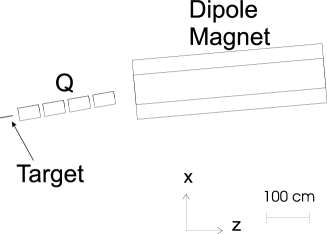
Figure 5: Beam line optics for high energy narrow band beam

The secondary pions from the target are focused by the following 4 Q magnets and bent by 10^∘ by a dipole magnet. The optics is not fully optimized. Several tens of $\%$ increase in flux could be expected by tuning the size or field of the Q and bending magnets, the position of the target etc.

In Fig. 6, some typical spectra obtained by the MC simulations are plotted. Spectra with a narrow peak structure are generated. The peak has a sharper edge in the high-energy side than in the low-energy side. The trailing edge in the low-energy side comes from pions with finite angle. We observe a small secondary peak at an energy about twice the primary peak position. The second peak comes from Kaon decays. In the left-hand-side figure, we show the flux of the neutrino at 2,100 km away from HIPA in units of $10^{4}$/400MeV/cm²/year, where $10^{21}$ POT is assumed for one-year operation. Three types of the NBB where peak energy is at about 3, 5, 8 GeV, and the high-energy WBB spectra are shown. The right-side figures show the expected number of $\nu_{\mu}$ CC events par year, in the absence of neutrino oscillation, for a 100 kton detector. The cross section has been obtained by assuming that the target detector made of water.

Figure 6: Typical spectra of narrow band beams. The left figure shows the $\nu_{\mu}$ flux and the right one gives the number of $\nu_{\mu}$ charged current interactions in the absence of oscillation at $L=2,100$ km. The solid, dashed and dotted histograms are 3, 5 and 8 GeV NBB, respectively. The thin solid histograms show the WBB spectra for comparison.

Figure 7: Composition of neutrino species for a typical NBB. Solid, dashed, dotted and dot-dashed histograms correspond to $\nu_{\mu}$, $\nu_{e}$, $\overline{\nu}_{\mu}$ and $\overline{\nu}_{e}$, respectively. The left and right figures shows 5 GeV $\nu_{\mu}$ and $\overline{\nu}_{\mu}$ beam, respectively.

Spectra for each neutrino species in the 5 GeV $\nu_{\mu}$ and $\overline{\nu}_{\mu}$ beams are shown in Fig. 7. The flux ratio of $\nu_{e}$($\overline{\nu}_{e}$) to $\nu_{\mu}(\overline{\nu}_{\mu}$) is $0.9\%$ ($0.8\%$) in total, and $0.2\%$ ($0.1\%$) at the peak energy for $\nu_{\mu}$ ($\overline{\nu}_{\mu}$) beam. In the left figure, we show the $\nu_{\nu},\nu_{e},\overline{\nu}_{\mu}$ and $\overline{\nu}_{e}$ spectrum of the NBB $\nu_{\mu}$ beam, while in the right figure the corresponding spectrum are shown for the NBB $\overline{\nu}_{\mu}$ beam. The number of wrong-sign $\overline{\nu}_{\mu}$ ($\nu_{\mu}$) CC interactions in $\nu_{\mu}$ ($\overline{\nu}_{\mu}$) beam is about $0.4\%$ ($4\%$) of the right-sign interactions. Although the flux of the $\nu_{\mu}$ beam and the $\overline{\nu}_{\mu}$ beam are almost the same, as well as the fraction of contaminated neutrino flux, the $\overline{\nu}_{\mu}$ beam suffers from 10 times higher wrong-sign events because of a factor of 3 smaller $\overline{\nu}_{\mu}$ CC interactions than the $\nu_{\mu}$ CC interactions off water target at these energies.

Table 4: Expected number of interactions of $\nu_{\mu}$ NBB. Assumed parameters are hierarchy I, $\delta m^{2}_{{}_{\rm ATM}}=3.5\times 10^{-3}$ eV², $\sin^{2}2\theta_{{}_{\rm ATM}}=1.0$, $\delta m^{2}_{{}_{\rm SOL}}=10\times 10^{-5}$ eV², $\sin^{2}2\theta_{{}_{\rm SOL}}=0.8$, $\sin^{2}2\theta_{{}_{\rm CHOOZ}}=0.06$, $\delta_{{}_{\rm MNS}}=0^{\circ}$ and $\rho=3$ g/cm³. First and second lines for each set of baseline length and the peak energy indicate the number of interactions without and with oscillation, respectively.

$L$	$E_{\rm peak}$	$\nu_{\mu}$ CC	$\overline{\nu}_{\mu}$ CC	$\nu_{e}$ CC	$\overline{\nu}_{e}$ CC	$N_{\rm NC}$
300km	3GeV	7495.	43.0	55.0	0.90	2540.9
		5903.	22.0	105.0	1.20	2540.9
	6GeV	13321.	44.0	82.0	1.90	4457.4
		12400.	21.0	110.0	1.70	4457.4
700km	3GeV	1376.	7.9	10.1	0.17	466.7
		382.	3.8	43.9	0.28	466.7
	6GeV	2446.	8.1	15.0	0.35	818.7
		1699.	3.5	40.6	0.36	818.7
1,200km	3GeV	468.	2.7	3.4	0.05	158.8
		85.	0.8	18.1	0.13	158.8
	6GeV	833.	2.7	5.1	0.12	278.6
		297.	1.1	25.3	0.13	278.6
2,100km	3GeV	153.	0.9	1.1	0.02	51.9
		119.	0.5	2.4	0.05	51.9
	6GeV	272.	0.9	1.6	0.04	91.0
		47.	0.4	13.2	0.06	91.0

Table 5: Expected number of interactions of $\overline{\nu}_{\mu}$ NBB. Assumed parameters are the same as in Table 4.

$L$	$E_{{\rm peak}}$	$\nu_{\mu}$ CC	$\overline{\nu}_{\mu}$ CC	$\nu_{e}$ CC	$\overline{\nu}_{e}$ CC	$N_{\rm NC}$
300km	3GeV	160.0	2871.0	4.0	12.7	1184.7
		66.0	2261.0	4.9	33.6	1184.7
	6GeV	141.0	4076.0	6.7	13.3	1584.8
		77.0	3793.6	5.4	22.4	1584.8
700km	3GeV	29.4	527.0	0.7	2.4	217.6
		13.9	136.0	1.1	16.6	217.6
	6GeV	25.9	748.6	1.2	2.5	291.1
		11.5	518.5	1.2	10.8	291.1
1,200km	3GeV	0.0	179.0	0.2	0.8	74.0
		3.5	28.0	0.5	7.0	74.0
	6GeV	8.8	254.7	0.4	0.8	99.1
		3.4	88.1	0.5	7.5	99.1
2,100km	3GeV	3.2	58.6	0.1	0.3	24.2
		1.9	47.6	0.2	0.8	24.2
	6GeV	2.8	83.1	0.1	0.3	32.3
		1.5	12.9	0.2	4.1	32.3

The results of the simulations are summarized in Table 4 and Table 5. In Table 4, we show the expected number of CC and NC events for the 3 GeV and 6 GeV $\nu_{\mu}$ NBB’s for 100 kton$\cdot$year (10²¹POT) at four typical distances, 300 km, 700km, 1,200 km, and 2,100km from HIPA. The upper numbers in each row and column show the numbers of events without oscillations, while the lower numbers are calculated by using the three neutrino model for the following parameters :

$$\left(~{}~{}\delta m^{2}_{{}_{\rm ATM}},~{}~{}~{}~{}~{}\delta m^{2}_{{}_{\rm SOL}},~{}~{}~{}\sin^{2}2\theta_{{}_{\rm ATM}},\sin^{2}2\theta_{{}_{\rm SOL}},\sin^{2}2\theta_{{}_{\rm CHOOZ}},\delta_{{}_{\rm MNS}}\right)$$ (3.1)

$$= \left(3.5\times 10^{-3},1.0\times 10^{-4},~{}~{}1.0,~{}~{}~{}~{}~{}~{}~{}~{}0.8,~{}~{}~{}~{}~{}~{}~{}~{}0.06,~{}~{}~{}~{}~{}~{}~{}~{}~{}~{}0^{\circ}~{}~{}~{}\right)$$

with the neutrino mass hierarchy I and for a constant matter density of $\rho=3$ g/cm³. Because all the three neutrinos have identical NC interactions, the two numbers are identical in $N_{\rm NC}$ column. All the upper numbers simply follow the $1/L^{2}$ rule of the flux at a distance $L$.

In Table 5, we show the corresponding numbers for the $\overline{\nu}_{\mu}$ NBB’s. The number of expected events are about a factor of 3 smaller than the corresponding ones in Table 4 because of the smaller CC and NC interactions of $\overline{\nu}_{\mu}$ off nucleus target.

Details of all the NBB’s generated for this study are available from [41].

3.4 Parameterization of the high-energy NBB

In the numerical studies of the next section, we make the following parameterization of the $\nu_{\mu}$ NBB with a single peak at $E_{\nu}=E_{\rm peak}$:

$$MN_{A}\Phi(E_{\nu})\sigma^{\rm CC}_{\mu}(E_{\nu}) = f(E_{\rm peak})\left(\frac{E_{\nu}}{E_{\rm peak}}\right)^{b(E_{\rm peak})-1}\left(\displaystyle\frac{\sigma_{\mu}^{\rm CC}(E_{\nu})}{\sigma_{e}^{\rm CC}(E_{\nu})}\right)\,,$$ (3.2)

where $E_{\nu}$ is running from 0 to $E_{\rm peak}$, and $f(E_{\rm peak})$ and $b(E_{\rm peak})$ are parameterized as

$$f(E_{\rm peak}) = 3.3E_{\rm peak}^{2}-76.8E_{\rm peak}+520\,,$$ (3.3a)

$$b(E_{\rm peak}) = 20.3E_{\rm peak}^{-1.4}+2.8\,,$$ (3.3b)

where $E_{\rm peak}$ is measured as unit of GeV. $M=100$ kton stands for the mass of the detector, $N_{A}=6.017\times 10^{23}$ is the Avogadro number, $\Phi(E_{\nu})$ is the flux (in units of /GeV/cm²/10²¹POT) at $L=2,100$ km. The $\sigma_{\mu}^{\rm CC}$ and $\sigma_{e}^{\rm CC}$ are, respectively, the $\nu_{\mu}$ and $\nu_{e}$ CC cross sections per nucleon off water target [42], and their ratio is approximately given by

$$\sigma_{\mu}^{\rm CC}(E_{\nu})/\sigma_{e}^{\rm CC}(E_{\nu}) \simeq \left\{\begin{array}[]{l}1.0-0.056E_{\nu}^{-0.48}~{}~{}~{}~{}(0.7~{}{\hbox to0.0pt{\lower 3.5pt\hbox{$\mathchar 0\relax\sim$}\hss}\raise 1.0pt\hbox{$<$}}\,E_{\nu})\\ 0.83+0.16E_{\nu}~{}~{}~{}~{}(0.3~{}{\hbox to0.0pt{\lower 3.5pt\hbox{$\mathchar 0\relax\sim$}\hss}\raise 1.0pt\hbox{$<$}}\,E_{\nu}~{}{\hbox to0.0pt{\lower 3.5pt\hbox{$\mathchar 0\relax\sim$}\hss}\raise 1.0pt\hbox{$<$}}\,0.7)\\ 0.879(E_{\nu}-m_{\mu})/(0.3-m_{\mu})~{}~{}~{}~{}(m_{\mu}~{}{\hbox to0.0pt{\lower 3.5pt\hbox{$\mathchar 0\relax\sim$}\hss}\raise 1.0pt\hbox{$<$}}\,E_{\nu}~{}{\hbox to0.0pt{\lower 3.5pt\hbox{$\mathchar 0\relax\sim$}\hss}\raise 1.0pt\hbox{$<$}}\,0.3)\end{array}\right.$$ (3.7)

where $m_{\mu}=0.11$ GeV represents the muon mass. This parameterization allows us to study the effects of changing the peak energy of the NBB continuously. We show in Fig. 8 our parameterizations of the NBB neutrino spectra by thick solid curves for several peak energies. For comparison, the corresponding original NBB spectra are shown by histograms. The parameterization reproduces well the main part of the $\nu_{\mu}$ NBB’s. Because it does not account for the secondary high-energy peak from $K^{+}\rightarrow\mu^{+}\nu_{\mu}$ decays (see Fig. 6), we check that our main conclusions are not affected by those details (especially the background from $\nu_{\tau}$ CC events).

We have not made parameterizations for the secondary ($\bar{\nu}_{\mu},\nu_{e},\bar{\nu}_{e}$) beams. In the following analysis we use the MC generated secondary beams at discrete energies ($E_{\rm peak}$) [41] and make interpolation for the needed $E_{\rm peak}$ values. Fluxes at different distances and for different species are obtained easily by multiplying the (2100 km/$L$)² flux factor and the ratio of the cross section at a given $E_{\nu}$.

Figure 8: The NBB’s from HIPA (histograms), and our parameterization (solid lines). The horizontal axis is the neutrino energy $(E_{\nu})$ and the vertical axis is the beam flux times $E_{\nu}$.

4 Results

In this section we present results of our numerical studies on physics potential of VLBL experiments by using the NBB’s from HIPA.

First, we present our basic strategy of the analysis and explain our simplified treatments of signals and backgrounds, and those of statistical and systematic errors. In the next subsection, we give our reference predictions for the results that may be obtained from the LBL experiment with HIPA and SK $(L=295$km$)$. In the latter two subsections, we give results of $L=2,100$ km and $L=1,200$ km, respectively.

4.1 Signals, backgrounds and systematic errors

In order to explore the physics potential of a VLBL experiment with HIPA at several base-line lengths, we make the following simple treatments in estimating the signals and the backgrounds of a future experiment. For a detector we envisage :

• A 100 kton-level water-$\check{\rm C}$erenkov detector which has a capability of distinguish $e^{\pm}$ CC events from $\mu^{\pm}$ CC events, but does not distinguish their charges.

• We do not require capability of the detector to reconstruct the neutrino energy.

Although water-$\check{\rm C}$erenkov detectors have the capability of measuring the three-momentum of the produced $\mu^{\pm}$ and $e^{\pm}$ as well as a part of hadronic activities, we do not make use of those information in our simplified analysis. Instead we use only the total numbers of the produced $\mu^{\pm}$ and $e^{\pm}$ events from a NBB with a given peak energy. For each base-line length $L$, we study the impacts of splitting the assumed total experiment exposure of 1000 kton$\cdot$year (with $10^{21}$ POT/year) into equi-partitioned runs of NBB’s at several peak energies. We find that the use of two different-energy NBB’s improves the physics resolving power of the experiment significantly, but we have not found further improvements by splitting the experiment into more than two NBB’s. We therefore choose two appropriate NBB’s at each $L$, whose peak energies are chosen to make physics outputs (such as sensitivity to the neutrino mass hierarchy, $\sin^{2}2\theta_{{}_{\rm CHOOZ}}$ and $\delta_{{}_{\rm MNS}}$ angles) significant. Optimum choice of NBB’s should depend on the model parameters

$$\left(~{}\delta m^{2}_{{}_{\rm ATM}}\,,~{}\delta m^{2}_{{}_{\rm SOL}}\,,~{}\sin^{2}2\theta_{{}_{\rm ATM}}\,,~{}\sin^{2}2\theta_{{}_{\rm SOL}}\,,~{}\sin^{2}2\theta_{{}_{\rm CHOOZ}}\,,~{}\delta_{{}_{\rm MNS}}~{}\right)\,,$$ (4.1)

especially on $\delta m^{2}_{{}_{\rm ATM}}$ and $\sin^{2}2\theta_{{}_{\rm ATM}}$, which will be measured more accurately by K2K [3], MINOS [16] and by HIPA-to-SK [19] in the future. All our major findings will not be affected by such details as long as appropriate NBB’s are chosen according to the data available at the time of the VLBL experiment.

The signals of our analysis are the numbers of $\nu_{\mu}$ CC events and those of $\nu_{e}$ CC events from the $\nu_{\mu}$ beam. They are calculated as

$$N(\mu,E_{\rm peak},L)=MN_{A}\int_{0}^{E_{\rm peak}}dE_{\nu}\Phi(E_{\rm peak})\sigma^{\rm CC}_{\mu}P_{\nu_{\mu}\rightarrow\nu_{\mu}}\,,$$ (4.2)

$$N(e,E_{\rm peak},L)=MN_{A}\int_{0}^{E_{\rm peak}}dE_{\nu}\Phi(E_{\rm peak})\sigma^{\rm CC}_{e}P_{\nu_{\mu}\rightarrow\nu_{e}}\,,$$ (4.3)

where the flux at a distance $L$ is calculated from the parameterization at $L=2,100$ km eq.(3.2) by multiplying the scale factor (2,100 km/$L$)². The cross sections are obtained by assuming a pure water target. At low $E_{\nu}$, the ratio of $\nu_{e}$ and $\nu_{\mu}$ CC cross sections is significant by different from unity, see eq.(3.7). Because of the vanishing of the NBB flux at low energies, our results are insensitive to the lower edge of the $E_{\nu}$ integration region. The probabilities $P_{\nu_{\mu}\rightarrow\nu_{\mu}}$ and $P_{\nu_{\mu}\rightarrow\nu_{e}}$ are calculated for the following model parameters ;

$$\sin^{2}2\theta_{{}_{\rm ATM}} = 1.0\,,~{}~{}~{}~{}~{}\delta m^{2}_{{}_{\rm ATM}}=3.5\times 10^{-3}~{}{\rm eV}^{2}\,,$$ (4.4a)

$$\sin^{2}2\theta_{{}_{\rm SOL}} = 0.8\,,~{}~{}~{}~{}~{}\delta m^{2}_{{}_{\rm SOL}}=10\times 10^{-5}~{}{\rm eV}^{2}\,,$$ (4.4b)

$$\sin^{2}2\theta_{{}_{\rm CHOOZ}} = 0.00\,,~{}0.02\,,~{}0.04\,,~{}0.06\,,~{}0.08\,,~{}0.10\,,$$ (4.4c)

$$\delta_{{}_{\rm MNS}} = 0^{\circ}\,,90^{\circ}\,,180^{\circ}\,,270^{\circ}\,,$$ (4.4d)

for the neutrino mass hierarchy I

$$\delta m^{2}_{13}=\delta m^{2}_{{}_{\rm ATM}}>0\,,~{}~{}~{}\delta m^{2}_{12}=\delta m^{2}_{{}_{\rm SOL}}>0\,,~{}~{}~{}~{}~{}({\rm hierarchy~{}I~{}})\,,$$ (4.5)

and for a constant matter density

$$\rho=3~{}{\rm g/cm}^{3},$$ (4.6)

throughout the base-line. We show in Fig. 9 the oscillation probabilities calculated for the above parameters, (at $\sin^{2}2\theta_{{}_{\rm CHOOZ}}=0.1$ and $\delta_{{}_{\rm MNS}}=270^{\circ}$ ) at three base-line lengths, $L=295$ km (SK), $L=1,200$ km and $L=2,100$ km. The NBB flux ($\times E_{\nu}$) chosen for our analysis are overlayed in each figure. We use the result at SK ($L=295$ km) expected for the low-energy NBB with $\langle p_{\pi}\rangle=2$ GeV as a reference.

Figure 9: The neutrino oscillation probabilities at (a) $L=295$ km, (b)$L=1,200$ km and (c) $L=2,100$ km calculated for the parameter values ; $\sin^{2}2\theta_{{}_{\rm ATM}}=1.0,~{}\delta m^{2}_{{}_{\rm ATM}}=3.5\times 10^{-3}{\rm eV}^{2},~{}\sin^{2}2\theta_{{}_{\rm SOL}}=0.8,~{}\delta m^{2}_{{}_{\rm SOL}}=10\times 10^{-5}{\rm eV}^{2},~{}\sin^{2}2\theta_{{}_{\rm CHOOZ}}=0.1,~{}\delta_{{}_{\rm MNS}}=270^{\circ}$ and $\rho=3$ g/cm³ with the hierarchy I. Overlayed are the NBB’s (flux times energy) used in our analysis.

The following background contributions to the ‘$\mu$’ and the ‘$e$’ events are accounted for :

$$N(\mu,E_{\rm peak},L)_{\rm BG} = N(\mu;\overline{\nu}_{\mu}{\rm CC})+N(\mu;\nu_{\tau}{\rm CC}:\tau\rightarrow\mu),$$ (4.7)

$$N(e,E_{\rm peak},L)_{\rm BG} = N(e;\nu_{e}{\rm CC})+N(e;\nu_{\tau}{\rm CC}:\tau\rightarrow e)+N(e;{\rm NC})$$ (4.8)

$$~{}~{}+N(e;\nu_{\tau}{\rm CC}:\tau\rightarrow{\rm hadrons}).$$

Here $\overline{\nu}_{\mu}$ CC and $\nu_{e}$ CC contributions are calculated by interpolating the numerical integrations

$$N(l;\stackrel{{\scriptstyle(-)}}{{\nu_{l}}}{\rm CC})=MN_{A}\int dE_{\nu}\Phi_{\stackrel{{\scriptstyle(-)}}{{\nu_{l}}}}(E_{\rm peak})\sigma_{\stackrel{{\scriptstyle(-)}}{{\nu_{l}}}}^{\rm CC}P_{\stackrel{{\scriptstyle(-)}}{{\nu_{l}}}\rightarrow\stackrel{{\scriptstyle(-)}}{{\nu_{l}}}}$$ (4.9)

for the discrete set of the MC simulations [41]. Here $\Phi_{\stackrel{{\scriptstyle(-)}}{{\nu_{\mu}}}}(E_{\rm peak})$ and $\Phi_{\nu_{e}}(E_{\rm peak})$ stand for, respectively, the MC generated secondary $\overline{\nu}_{\mu}$ and $\nu_{e}$ flux of the primarily $\nu_{\mu}$ beam. The survival probabilities are calculated for the same set of the model parameters, eq.(4.1). We find that contributions from oscillations from the background beams, such as $\overline{\nu}_{e}\rightarrow\overline{\nu}_{\mu}$, are negligibly small and hence they are not counted. The contributions from $\tau$-lepton pure-leptonic decays are estimated as

$$N(l;\nu_{\tau}{\rm CC}:\tau\rightarrow l)=MN_{A}\int dE_{\nu}\Phi(E_{\rm peak})P_{\nu_{\mu}\rightarrow\nu_{\tau}}\sigma_{\nu_{\tau}}^{\rm CC}Br(\tau\rightarrow l\overline{\nu}_{l}\nu_{\tau})\,,$$ (4.10)

where we adopt $Br(\tau\rightarrow\mu\overline{\nu}_{\mu}\nu_{\tau})=0.1737$ and $Br(\tau\rightarrow e\overline{\nu}_{e}\nu_{\tau})=0.1783$ [43]. The 10 $\%$ errors in these branching fractions are accounted for as systematic errors. Because of the $\tau$-lepton threshold, $\tau$-backgrounds are significant only at high energies, NBB’s with $E_{\rm peak}~{}{\hbox to0.0pt{\lower 3.5pt\hbox{$\mathchar 0\relax\sim$}\hss}\raise 1.0pt\hbox{$>$}}\,$ 4 GeV. Because they receive contribution from the small high-energy secondary peak due to Kaon decays, we use the interpolation of the results obtained for discrete set of MC generated fluxes.

The ‘$e$’ events receive contributions from the NC events where produced $\pi^{0}$’s mimic electron shower in the water-$\check{\rm C}$erenkov detector. By using the estimations from the SK experiments, we adopt

$$N(e;{\rm NC})=MN_{A}\int dE_{\nu}\Phi(E_{\rm peak})\sigma_{\nu_{\mu}}^{\rm NC}P_{e/{\rm NC}}$$ (4.11)

with

$$P_{e/{\rm NC}}=0.0055\pm 0.00055\,.$$ (4.12)

The error in the above $e/{\rm NC}$ mis-identification probability is accounted for as a systematic error. The last term in eq.(4.8) accounts for the probability that the $\nu_{\tau}$ CC events with hadronic $\tau$-decays are counted as $e$-like events. In the absence of detailed study of such backgrounds, we use the same misidentification probability for the NC events eq.(4.12) and obtain

$$N(e;\nu_{\tau}{\rm CC}:\tau \rightarrow {\rm hadrons})=$$ (4.13)

$$MN_{A}\int dE_{\nu}\Phi(E_{\rm peak})P_{\nu_{\mu}\rightarrow\nu_{\tau}}\sigma_{\nu_{\tau}}^{\rm CC}Br(\tau\rightarrow\nu_{\tau}{\rm hadrons})P_{e/{\rm NC}}\,.$$

If the small misidentification probability of eq.(4.12) holds even for $\tau\rightarrow$ hadron events, their background is only at the 2 $\%$ level of the $\tau\rightarrow e$ background, $N(e;\nu_{\tau}{\rm CC}:\tau\rightarrow e)$, and hence can safely be neglected.

In addition, we account for the following two effects as the major part of the systematic uncertainty in the VLBL experiments. One is the uncertainty in the total flux of the neutrino beam, for which we adopt the estimate,

$$f_{{}_{\rm FLUX}}=1\pm 0.03\,,$$ (4.14)

common for all the high-energy NBB’s. We allocate an independent flux uncertainty of 3$\%$ for the low-energy NBB used for the SK experiment ($L=295$ km) since it uses different optics. Finally, we allocate 3.3 $\%$ uncertainty in the matter density along the base-line. In our simplified analysis, we use

$$\rho=3.0\pm 0.1~{}{\rm g/cm^{3}}$$ (4.15)

as a representative density and the uncertainty.

(a) $L=2,100$ km

		$N_{\rm signal}$	$N_{\rm BG}$			$N_{\rm tot}$	$\frac{N_{\rm signal}}{N_{\rm tot}}$
			beams	$\nu_{\tau}$ CC	NC
NBB ($E_{\rm peak}=6$ GeV)	$N(\mu)$	202.5	2.2	15.2	$-$	219.9	.92
500kton$\cdot$year	$N(e)$	126.5	7.3	15.9	3.3	153.0	.83
NBB ($E_{\rm peak}=4$ GeV)	$N(\mu)$	612.5	2.2	3.5	$-$	618.2	.99
500kton$\cdot$year	$N(e)$	66.4	8.5	3.7	2.6	81.2	.82

(b) $L=1,200$ km

		$N_{\rm signal}$	$N_{\rm BG}$			$N_{\rm tot}$	$\frac{N_{\rm signal}}{N_{\rm tot}}$
			beams	$\nu_{\tau}$ CC	NC
NBB ($E_{\rm peak}=5$ GeV)	$N(\mu)$	490.1	2.2	8.7	$-$	501.0	.98
500kton$\cdot$year	$N(e)$	239.1	10.5	9.0	9.4	268.0	.89
NBB ($E_{\rm peak}=3$ GeV)	$N(\mu)$	413.8	2.3	0.0	$-$	416.1	.99
500kton$\cdot$year	$N(e)$	186.1	4.8	0.0	5.6	196.5	.95

(c) $L=295$ km

		$N_{\rm signal}$	$N_{\rm BG}$			$N_{\rm tot}$	$\frac{N_{\rm signal}}{N_{\rm tot}}$
			beams	$\nu_{\tau}$ CC	NC
NBB ($\langle p_{\pi}\rangle=2$ GeV)	$N(\mu)$	464.9	7.8	0.0	$-$	472.7	.98
100kton$\cdot$year	$N(e)$	161.3	22.0	0.0	7.4	190.7	.85

Table 6: Expected signals and backgrounds for $\mu$-like and $e$-like events. The results are shown for the parameters of eq.(4.3) at $\delta_{{}_{\rm MNS}}=270^{\circ}$, (a) 500kton$\cdot$year at $L=2,100$ km, (b) 500kton$\cdot$year at $L=1,200$ km, (c) 100kton$\cdot$year at $L=295$ km.

Typical numbers of expected signals and backgrounds are tabulated in Table 6 for the parameter set of eq.(4.1) at $\sin^{2}2\theta_{{}_{\rm CHOOZ}}=0.1$ and $\delta_{{}_{\rm MNS}}=270^{\circ}$. The numerical values are given for the following sets of experimental conditions ;

(4.19)

We note here that 100 kton$\cdot$year at $L=295$ km is what SK can gather in approximately 5 years with $10^{21}$ POT par year. 500 kton$\cdot$year at longer distances can be accumulated in 5 years for a 100 kton detector with the same intensity beam.

A few remarks are in order. A 100 kton-level detector at $L=2,100$ km or 1,200 km can detect comparable numbers of $\mu$-like and $e$-like events as SK (22.5 kton) at $L=295$ km. The backgrounds due to secondary beams (mostly from the $\nu_{e}$ beam ) are significant in all cases for the $e$-like events. The NC background for the $e$-like events remain small at high energies if the estimate eq.(4.12) obtained from the K2K experiment at SK remain valid. We may expect gradual increase in the misidentification probability $P_{e/{\rm NC}}$ at high energies as the mean multiplicity of $\pi^{0}$ and charged particles grow. Finally the $\tau$-decay background can be significant only for NBB’s with $E_{\rm peak}~{}{\hbox to0.0pt{\lower 3.5pt\hbox{$\mathchar 0\relax\sim$}\hss}\raise 1.0pt\hbox{$>$}}\,5$ GeV. If a detector is capable of distinguishing $\tau$-events from the $\nu_{e}$ and $\nu_{\mu}$ CC events, the overall fit quality improves slightly in the three-neutrino model, because the constraint $P_{\nu_{\mu}\rightarrow\nu_{e}}+P_{\nu_{\mu}\rightarrow\nu_{\mu}}+P_{\nu_{\mu}\rightarrow\nu_{\tau}}=1$ implies that the information obtained from the $P_{\nu_{\mu}\rightarrow\nu_{e}}$ measurement always diminishes by contaminations from the $\tau$-events. As remarked in section 3.4, the $\nu_{\tau}$ CC event rates have been corrected for the high-energy secondary peak contributions by using the original MC generated NBB spectrum [41].

4.2 Results for $L=295$ km

Figure 10: CP phase dependence of $N(e)$ and $N(\mu)$ at SK($L=295$ km) for 100kton$\cdot$year with the NBB($\langle p_{\pi}\rangle=2$ GeV). $\delta_{{}_{\rm MNS}}=0^{\circ}$ (solid-circle), $90^{\circ}$ (solid-square), $180^{\circ}$ (open-circle), and $270^{\circ}$ (open-square). The results are shown for $\sin^{2}2\theta_{{}_{\rm ATM}}=1.0$, $\delta m^{2}_{{}_{\rm ATM}}=3.5\times 10^{-3}\mbox{eV${}^{2}$}$, $\sin^{2}2\theta_{{}_{\rm SOL}}=0.8$, $\delta m^{2}_{{}_{\rm SOL}}=10\times 10^{-5}\mbox{eV${}^{2}$}$, $\sin^{2}2\theta_{{}_{\rm CHOOZ}}=0.1$, and $\rho$ = 3 g/cm³. The predictions for the four types of the neutrino mass hierarchies (Fig. 1) are depicted as I, II, III and IV.

In Fig. 10 we show the number of $\nu_{\mu}$ CC events, $N(\mu)$, and that of $\nu_{e}$ CC events, $N(e)$, expected at SK ($L=295$ km) for 100 kton$\cdot$year. The NBB with $\langle p_{\pi}\rangle=2$ GeV, NBB($\langle p_{\pi}\rangle=2$ GeV), with $10^{21}$POT per year has been assumed for simplicity. The three-neutrino model parameters of eq.(4.1) at $\sin^{2}2\theta_{{}_{\rm CHOOZ}}=0.1$ are assumed, and we take $\rho=3$g/cm³, eq.(4.6). The predictions then depend only on the CP phase parameter $\delta_{{}_{\rm MNS}}$, and when we vary $\delta_{{}_{\rm MNS}}$ from $0^{\circ}$ to $360^{\circ}$, we have a circle on the plane of $N(\mu)$ vs $N(e)$. The four representative cases, $\delta_{{}_{\rm MNS}}=0^{\circ},90^{\circ},180^{\circ}$ and $270^{\circ}$, are marked by solid-circle, solid-square, open-circle, and open-square, respectively. The four possible mass hierarchy cases of Fig. 1 are depicted as I, II, III and IV.

Only the expected event-numbers from the $\nu_{\mu}$ beam, eq.(4.2) and eq.(4.3), are counted in Fig. 10, so that we can read off the ultimate sensitivity of the experiment from the figure. Statistical errors for such an experiment are shown for the $\delta_{{}_{\rm MNS}}=270^{\circ}$ point in the mass hierarchy I circle. We can learn from the figure that if we know all the parameters of the three-neutrino model except for the mass hierarchy and if we know the neutrino-beam flux exactly, then there is a possibility of distinguishing the mass hierarchy I from III. In practice, the LBL experiment between HIPA and SK can constrain mainly $\delta m^{2}_{{}_{\rm ATM}}$ and $\sin^{2}2\theta_{{}_{\rm ATM}}$ from $N(\mu)$, and $\sin^{2}2\theta_{{}_{\rm CHOOZ}}$ from $N(e)$ [19]. Fig. 10 shows that those measurements should suffer from uncertainties in the remaining parameters of the three-neutrino model, the neutrino mass hierarchy cases and $\delta_{{}_{\rm MNS}}$, as are explicitly shown, as well as on the solar-neutrino oscillation parameters, $\delta m^{2}_{{}_{\rm SOL}}$ and $\sin^{2}2\theta_{{}_{\rm SOL}}$. Next generation of the solar-neutrino observation experiments [44] and KamLAND experiment [45] may further constrain the latter two parameters, but the mass-hierarchy (between I and III) and $\delta_{{}_{\rm MNS}}$ should be determined by the next generation of accelerator-based LBL experiments.

It is hence necessary that all the results from the LBL experiment between HIPA and SK [19] should be expressed as constraints on the three primary parameters, $\delta m^{2}_{{}_{\rm ATM}}$, $\sin^{2}2\theta_{{}_{\rm ATM}}$, and $\sin^{2}2\theta_{{}_{\rm CHOOZ}}$, which depend slightly on the three remaining parameters of the three-neutrino model, $\delta m^{2}_{{}_{\rm SOL}}$, $\sin^{2}2\theta_{{}_{\rm SOL}}$ and $\delta_{{}_{\rm MNS}}$, as well as on the mass-hierarchy cases. In the following subsections, we show that the data obtained from the LBL experiment between HIPA and SK ($L=295$ km) are useful in determining the neutrino mass hierarchy, and in some cases even $\delta_{{}_{\rm MNS}}$, when they are combined with the data from a VLBL experiments ($L=2,100$ km or 1,200 km) with higher-energy neutrino beams from HIPA.

Before moving on to studying physics potential of VLBL experiments, it is worth noting that the predictions for the mass hierarchy IV in Fig. 10 represents the prediction for the $\overline{\nu}_{\mu}\rightarrow\overline{\nu}_{\mu},\overline{\nu}_{e}$ oscillation probabilities in the hierarchy I, according to the theorem eq.(2.4), once the scales are connected by the factor $\sigma(\overline{\nu}_{l}N)/\sigma(\nu_{l}N)$. By comparing the $\delta_{{}_{\rm MNS}}$ dependences of the circle I and circle IV, we can clearly see that $P_{\nu_{\mu}\rightarrow\nu_{e}}$ and $P_{\overline{\nu}_{\mu}\rightarrow\overline{\nu}_{e}}$ interchange approximately by exchanging $\delta_{{}_{\rm MNS}}=90^{\circ}$ and $270^{\circ}$. The comparison of $\nu_{\mu}$ and $\overline{\nu}_{\mu}$ oscillation experiments at around $L=295$ km hence has a potential of discovering CP-violation in the lepton sector. However, determination of the $\delta_{{}_{\rm MNS}}$ angle by using the $\overline{\nu}_{\mu}$ beam from HIPA needs a much bigger detector than SK [19, 46].

4.3 Results for $L=2,100$ km

Fig. 11 shows the numbers of $\nu_{\mu}$ CC events and that of $\nu_{e}$ CC events expected at the base-line length of $L=2,100$ km from HIPA with 500 kton$\cdot$year. The expected signal event numbers are shown for (a) the NBB with $E_{\rm peak}=4$ GeV and for (b) the NBB with $E_{\rm peak}=6$ GeV. The parameters of the three neutrino model and the matter density are taken exactly the same as in Fig. 10 :

$$\sin^{2}2\theta_{{}_{\rm ATM}} = 1.0\,,~{}~{}~{}~{}~{}\delta m^{2}_{{}_{\rm ATM}}=3.5\times 10^{-3}~{}{\rm eV}^{2}\,,$$ (4.20a)

$$\sin^{2}2\theta_{{}_{\rm SOL}} = 0.8\,,~{}~{}~{}~{}~{}\delta m^{2}_{{}_{\rm SOL}}=10\times 10^{-5}~{}{\rm eV}^{2}\,,$$ (4.20b)

$$\sin^{2}2\theta_{{}_{\rm CHOOZ}} = 0.1\,,$$ (4.20c)

$$\delta_{{}_{\rm MNS}} = 0^{\circ}~{}-~{}360^{\circ}\,,$$ (4.20d)

$$\rho = 3~{}{\rm g/cm^{3}}\,.$$ (4.20e)

The predictions for the four neutrino mass hierarchy cases (Fig. 1) are shown by separate circles when the CP-phase angle $\delta_{{}_{\rm MNS}}$ is allowed to vary freely. The predictions for the four representative phase values are shown by solid-circle ($\delta_{{}_{\rm MNS}}=0^{\circ}$), solid-square ($90^{\circ}$), open-circle ($180^{\circ}$), and open-square ($270^{\circ}$).

Figure 11: CP phase dependence of $N(e)$ and $N(\mu)$ at $L=2100$ km for 500 kton$\cdot$year with (a) NBB($E_{\rm peak}=4$ GeV) and (b) NBB($E_{\rm peak}=6$ GeV). $\delta_{{}_{\rm MNS}}=0^{\circ}$ (solid-circle), $90^{\circ}$ (solid-square), $180^{\circ}$ (open-circle), and $270^{\circ}$ (open-square). The results are shown for $\delta m^{2}_{{}_{\rm ATM}}=3.5\times 10^{-3}\mbox{eV${}^{2}$}$, $\sin^{2}2\theta_{{}_{\rm ATM}}=1.0$, $\delta m^{2}_{{}_{\rm SOL}}=10\times 10^{-5}\mbox{eV${}^{2}$}$, $\sin^{2}2\theta_{{}_{\rm SOL}}=0.8$, $\sin^{2}2\theta_{{}_{\rm CHOOZ}}=0.1$, and $\rho=3$ g/cm³. The predictions for the four types of the neutrino mass hierarchies (Fig. 1) are depicted as I, II, III and IV.

Figure 12: $P_{\nu_{\mu}\rightarrow\nu_{\mu}}$ and $P_{\nu_{\mu}\rightarrow\nu_{e}}$ vs. $E_{\nu}$ (GeV) at $L=2,100$ km. Solid lines are for $\delta_{{}_{\rm MNS}}=0^{\circ}$, long-dashed lines are for $\delta_{{}_{\rm MNS}}=90^{\circ}$, short-dashed lines are for $\delta_{{}_{\rm MNS}}=180^{\circ}$, and dot-dashed line are for $\delta_{{}_{\rm MNS}}=270^{\circ}$.

When comparing with the $L=295$ km case (Fig. 10), it is most striking to find that the predictions for the $\nu_{e}$ CC events, $N(e)$, differs by a factor of 5 or even larger in magnitude between the neutrino mass hierarchy I and III. This is because of the enhancement of the matter effect at high energies as depicted in Fig. 3. This striking sensitivity of the probability $P_{\nu_{\mu}\rightarrow\nu_{e}}$ on the mass hierarchy cases is the bases of the capability of distinguishing the cases in VLBL experiments by using the HIPA beam. On the other hand, we will find that the 5 $\%$ level differences in $N(\mu)$ between the mass hierarchy cases are not useful for this purpose because $P_{\nu_{\mu}\rightarrow\nu_{\mu}}$ depends strongly on the parameters $\delta m^{2}_{{}_{\rm ATM}}$ and $\sin^{2}2\theta_{{}_{\rm ATM}}$, and also because $N(\mu)$ suffers from the neutrino-beam flux uncertainty eq.(4.14).

We have examined NBB’s with various peak energies, and find that the NBB with $E_{\rm peak}=6$ GeV (see Fig. 9) makes $N(e)$ largest while keeping $N(\mu)$ small for the atmospheric-neutrino oscillation parameter of eq.(4.20a). The ration $N(e)/N(\mu)$ can be as large as $1/2$ if $\sin^{2}2\theta_{{}_{\rm CHOOZ}}=0.1$ (eq.(4.20c)) for the hierarchy case I. The NBB with $E_{\rm peak}=4$ GeV is then chosen because it has the $\delta_{{}_{\rm MNS}}$ dependence of $N(e)$ which is ‘orthogonal’ to that of the $E_{\rm peak}=6$ GeV case. By comparing the hierarchy I circles of Fig. 11(a) and (b), we find that for the NBB with $E_{\rm peak}$ = 4 GeV, $N(e)$ is largest at around $\delta_{{}_{\rm MNS}}=180^{\circ}$ (open-circle) and smallest at around $\delta_{{}_{\rm MNS}}=0^{\circ}$ (solid-circle), whereas for the NBB with $E_{\rm peak}=6$ GeV, $N(e)$ is largest at around $\delta_{{}_{\rm MNS}}=270^{\circ}$ (open-square) and smallest at around $\delta_{{}_{\rm MNS}}=90^{\circ}$ (solid-square).

In order to understand the dependences of $N(\mu),N(e)$ on $E_{\rm peak}$ (the peak energy of the NBB) and on $\delta_{{}_{\rm MNS}}$, and in particular to probe the reason for this peculiar $\delta_{{}_{\rm MNS}}$-dependence of the expected number of $\nu_{e}$ CC events on $E_{\rm peak}$, we show in Fig. 12 the oscillation probabilities $P_{\nu_{\mu}\rightarrow\nu_{\mu}}$ and $P_{\nu_{\mu}\rightarrow\nu_{e}}$ plotted against the neutrino energy, $E_{\nu}$. The three plots in the left-hand-side are for $P_{\nu_{\mu}\rightarrow\nu_{\mu}}$ and the three in the right-hand-side are for $P_{\nu_{\mu}\rightarrow\nu_{e}}$. In all the plots, the predictions of the three-neutrino model with the parameters of eq.(4.3) are shown by thick lines for the neutrino mass hierarchy I. In the upper, middle and bottom figures, the predictions for the same parameters are shown by thin lines for the hierarchy II, III, and IV, respectively. In all the plots the predictions for $\delta_{{}_{\rm MNS}}=0^{\circ},90^{\circ},180^{\circ},270^{\circ}$ are shown by solid, long-dashed, short-dashed, and dot-dashed lines, respectively. It is clear from these figures that the transition probability $P_{\nu_{\mu}\rightarrow\nu_{e}}$ is more sensitive than the reduction probability $P_{\nu_{\mu}\rightarrow\nu_{\mu}}$ on the neutrino mass hierarchy and $\delta_{{}_{\rm MNS}}$. For the chosen parameters of eq.(4.3), $P_{\nu_{\mu}\rightarrow\nu_{\mu}}$ hits zero at around $E_{\nu}=6$ GeV at $L=2,100$ km, where the transition probability $P_{\nu_{\mu}\rightarrow\nu_{e}}$ becomes largest in the interval 4 GeV $<E_{\nu}<6$ GeV. Because the NBB with $E_{\rm peak}=6$ GeV is largest at the peak and has significant tail down to around $E_{\nu}$ = 4 GeV, see Fig. 9(c) for the NBB shape, we find largest $N(e)$ and smallest $N(\mu)$ for this NBB. At the same time we clearly see that in the interval 4 GeV $<E_{\nu}<$ 6 GeV, $P_{\nu_{\mu}\rightarrow\nu_{e}}$ is largest at $\delta_{{}_{\rm MNS}}=270^{\circ}$ (dot-dashed line), and smallest at $\delta_{{}_{\rm MNS}}=90^{\circ}$ (long-dashed line). Just below $E_{\nu}=4$ GeV the ordering between the $\delta_{{}_{\rm MNS}}=270^{\circ}$ (dot-dashed) curve and the $\delta_{{}_{\rm MNS}}=180^{\circ}$ (short-dashed) curves and that between the $\delta_{{}_{\rm MNS}}=0^{\circ}$ (solid) curve and the $\delta_{{}_{\rm MNS}}=90^{\circ}$ (long-dashed) curve is reversed. Consequently the NBB with $E_{\rm peak}=4$ GeV gives largest $N(e)$ at around $\delta_{{}_{\rm MNS}}=180^{\circ}$ and smallest $N(e)$ at around $\delta_{{}_{\rm MNS}}=0^{\circ}$, among the four representative $\delta_{{}_{\rm MNS}}$ angles. The overall normalization of $N(e)$ is smaller, and that of $N(\mu)$ is larger for NBB ($E_{\rm peak}=4$ GeV) than the predictions of NBB ($E_{\rm peak}=6$ GeV).

In Fig. 11, we show the statistical errors of the $N(\mu)$ and $N(e)$ measurements at 500 kton$\cdot$year on the $\delta_{{}_{\rm MNS}}=270^{\circ}$ point for the hierarchy case I. The size of the error bars suggest that a 100 kton-level detector is needed to explore the model parameters in VLBL experiments at $L\simeq$ 2,100 km. It also tells us that such detector has the potential of discriminating the neutrino mass hierarchies and constraining the $\delta_{{}_{\rm MNS}}$ angle in a certain region of the three-neutrino model parameter space. A more careful error analysis that accounts for backgrounds and systematic errors is given in the next subsection.

We are now ready to study the physics capability of such VLBL experiments in some detail. In Fig. 13, we show the expected numbers of signal events, $N(\mu)$ and $N(e)$, for the same NBB’s and for the same volume of 500 kton$\cdot$year as in Fig. 11. The circles of Fig. 11 are now made of 36 $\delta_{{}_{\rm MNS}}$ points, $\delta_{{}_{\rm MNS}}=n\times 10^{\circ}$ for $n=1$ to 36, for each set of the model parameters. The common parameters for all the points are

$$\sin^{2}2\theta_{{}_{\rm ATM}} = 1.0\,,~{}~{}\delta m^{2}_{{}_{\rm ATM}}=3.5\times 10^{-3}~{}{\rm eV}^{2}\,,$$ (4.21a)

$$\sin^{2}2\theta_{{}_{\rm CHOOZ}} = 0.00\,,~{}0.02\,,~{}0.04\,,~{}0.06\,,~{}0.08\,,~{}0.10\,,$$ (4.21b)

$$\delta_{{}_{\rm MNS}} = n\times 10^{\circ}~{}~{}(n=1~{}{\rm to}~{}36)\,,$$ (4.21c)

$$\rho = 3~{}{\rm g/cm^{3}}\,.$$ (4.21d)

The predictions for the six $\sin^{2}2\theta_{{}_{\rm CHOOZ}}$ cases eq.(4.21b) can be recognized as five circles and one point with decreasing $N(e)$ values, as $\sin^{2}2\theta_{{}_{\rm CHOOZ}}$ decreases from 0.1 to 0.0. The remaining two parameters are constrained by the solar-neutrino oscillation experiments, and we chose the following representative parameter sets for the three possible solutions to the solar-neutrino deficit anomaly :

$${\rm LMA}~{}~{}~{} : ~{}~{}~{}\sin^{2}2\theta_{{}_{\rm SOL}}=0.8\,,~{}~{}~{}~{}~{}~{}~{}~{}~{}~{}\delta m^{2}_{{}_{\rm SOL}}=\left\{\begin{array}[]{l}15\times 10^{-5}~{}{\rm eV}^{2}\,,\\ 5\times 10^{-5}~{}{\rm eV}^{2}\,,\end{array}\right.$$ (4.22c)

$${\rm SMA}~{}~{}~{} : ~{}~{}~{}\sin^{2}2\theta_{{}_{\rm SOL}}=7\times 10^{-3}\,,~{}~{}~{}\delta m^{2}_{{}_{\rm SOL}}=5\times 10^{-6}~{}{\rm eV}^{2}\,,$$ (4.22d)

$${\rm VO~{}}~{}~{}~{} : ~{}~{}~{}\sin^{2}2\theta_{{}_{\rm SOL}}=0.7\,,~{}~{}~{}~{}~{}~{}~{}~{}~{}~{}\delta m^{2}_{{}_{\rm SOL}}=7\times 10^{-11}~{}{\rm eV}^{2}\,.$$ (4.22e)

The predictions of the four types of the neutrino mass hierarchy, I, II, III, IV are indicated explicitly.

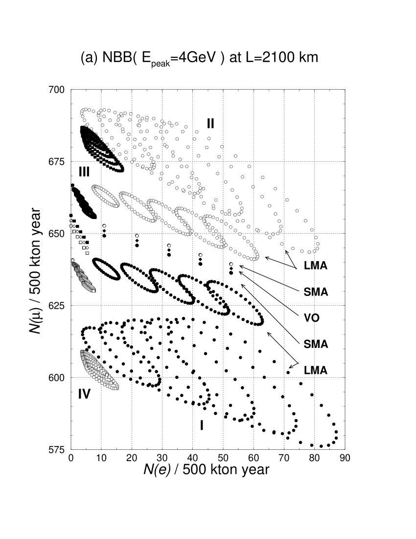
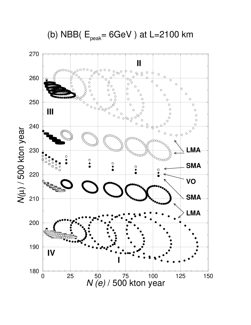
Figure 13: The neutrino parameter dependences of the expected numbers of $\nu_{e}$ CC and $\nu_{\mu}$ CC events, $N(e)$ and $N(\mu)$, respectively, for the NBB with $E_{\rm peak}=4$ GeV (a) and 6 GeV (b) with 500 kton$\cdot$year at $L=2,100$ km. The predictions are shown for the LMA, SMA, and VO scenarios of the solar neutrino oscillations and for the four neutrino mass hierarchies I to IV. All the numbers are calculated for $\delta m^{2}_{{}_{\rm ATM}}=3.5\times 10^{-3}$eV² and $\sin^{2}2\theta_{{}_{\rm ATM}}=1.0$ at $\sin^{2}2\theta_{{}_{\rm CHOOZ}}=0.02\times m$ ($m=0$ to 5) and $\delta_{{}_{\rm MNS}}=10^{\circ}\times n$ ($n=1$ to 36). The five larger circles in each hierarchy show the $\delta_{{}_{\rm MNS}}$ predictions of the LMA with $\delta m^{2}_{{}_{\rm SOL}}=15\times 10^{-5}$eV² and the five smaller circles are for the LMA with $\delta m^{2}_{{}_{\rm SOL}}=5\times 10^{-5}$eV², both for $m=1$ to 5. $\delta_{{}_{\rm MNS}}$-dependence is not recognized for the predictions of SMA and VO, and also at $\sin^{2}2\theta_{{}_{\rm CHOOZ}}=0$ ($m=0$). The VO predictions are the same for the hierarchy I and II, and III and IV.

The solid-circle points in Fig. 13 show the predictions of all the models with neutrino mass hierarchy I. They reside in the corner at large $N(e)$ and small $N(\mu)$. The five grand circles with smallest $N(\mu)$ give the predictions of the LMA solution for $\delta m^{2}_{{}_{\rm SOL}}=15\times 10^{-5}$ eV², and those with larger $N(\mu)$ are for the LMA with $\delta m^{2}_{{}_{\rm SOL}}=5\times 10^{-5}$ eV². It is clearly seen that the $\delta_{{}_{\rm MNS}}$ dependence (the size of the grand circles) is larger for larger $\delta m^{2}_{{}_{\rm SOL}}$ and for larger $\sin^{2}2\theta_{{}_{\rm CHOOZ}}$ as expected. It is worth pointing out that the LMA scenario with $\delta m^{2}_{{}_{\rm SOL}}=15\times 10^{-5}$ eV² predicts non-zero $N(e),N(e)\simeq 5$/500 kton$\cdot$year even when $\sin^{2}2\theta_{{}_{\rm CHOOZ}}=0$. This is because the ‘higher’ oscillation modes of the three-neutrino model grow as $\delta m^{2}_{{}_{\rm SOL}}/\delta m^{2}_{{}_{\rm ATM}}$ rises. The predictions of the SMA parameters appear just above the upper LMA grand circles, where the $\delta_{{}_{\rm MNS}}$ dependence (the size of the grand circle) diminishes to zero for each $\sin^{2}2\theta_{{}_{\rm CHOOZ}}$ value of eq.(4.21b). Just five solid-circle points appear in Fig. 13 (a) and (b) for the SMA parameters because the $\delta_{{}_{\rm MNS}}$-dependence diminishes as $\delta m^{2}_{{}_{\rm SOL}}/\delta m^{2}_{{}_{\rm ATM}}$ and $\sin^{2}2\theta_{{}_{\rm SOL}}$ are both significantly smaller than unity. This is expected from the Hamiltonian eq.(2.108h) that governs the neutrino oscillation in matter, because the $\delta_{{}_{\rm MNS}}$-dependence of observables diminished whenever the second terms proportional to $\delta m_{12}^{2}/\delta m_{13}^{2}$ are much smaller than the first term. The predictions of the VO parameters, which are given by the solid-diamonds, are shown just above those of the SMA parameters. Here the $\delta_{{}_{\rm MNS}}$ dependence vanishes because of the extreme smallness of $\delta m^{2}_{{}_{\rm SOL}}/\delta m^{2}_{{}_{\rm ATM}}$. With the same token, we cannot distinguish the VO predictions of the neutrino mass hierarchy I and II. Because the magnitude of $\delta m^{2}_{{}_{\rm SOL}}$ is so small, the sign of $\delta m^{2}_{12}=\pm\delta m^{2}_{{}_{\rm SOL}}$ does not have observable consequences in terrestrial LBL experiments.

The predictions of the four scenarios of the solar neutrino oscillations (VO, SMA, and two $\delta m^{2}_{{}_{\rm SOL}}$ cases of LMA in eq.(4.3)) with the neutrino mass hierarchy II ($\delta m^{2}_{12}=-\delta m^{2}_{{}_{\rm SOL}},\delta m^{2}_{13}=\delta m^{2}_{{}_{\rm ATM}}$) are shown by open-circle points, which are located in the corner of large $N(e)$ large $N(\mu)$. As explained above, the predictions of the VO scenario do not differ from those for the hierarchy I. The predictions of the SMA scenario appear slightly above those of VO. The two LMA scenarios predict larger $N(\mu)$ and give visible $\delta_{{}_{\rm MNS}}$ dependences, which lead to five grand circles each for the five discrete values of assumed $\sin^{2}2\theta_{{}_{\rm CHOOZ}}$. Again the $\delta_{{}_{\rm MNS}}$-dependence (the size of the grand circles) is larger for the large $\sin^{2}2\theta_{{}_{\rm CHOOZ}}$ and large $\delta m^{2}_{{}_{\rm SOL}}$. Summarizing the predictions of the four scenarios in the neutrino mass hierarchies I and II, both of which have $\delta m^{2}_{13}=\delta m^{2}_{{}_{\rm ATM}}>0$, $N(e)$ grows linearly with increasing $\sin^{2}2\theta_{{}_{\rm CHOOZ}}$ in all four scenarios and for both hierarchies. The predictions of the hierarchy II differ from those of the hierarchy I only by slightly larger $N(\mu)$ in each scenarios. The difference in $N(\mu)$ is largest in the LMA scenarios with $\delta m^{2}_{{}_{\rm SOL}}=15\times 10^{-5}$ eV², for which the hierarchy II predicts about 30 $\%$ (10 $\%$) larger $N(\mu)$ than the predictions of the hierarchy I for the NBB with $E_{\rm peak}=6$ GeV (4 GeV).

All the predictions of the hierarchy cases III and IV have very small $N(e)$, as we explained in section 2.4 for the hierarchy III. This is because the two mass hierarchies have $\delta m^{2}_{13}=-\delta m^{2}_{{}_{\rm ATM}}$ common. The predictions of the hierarchy III are shown by solid-squares and those of the hierarchy IV are shown by open-squares. As in the case of hierarchy I vs II, the predictions of the VO scenario do not show visible dependence on the sign of $\delta m^{2}_{12}=\pm\delta m^{2}_{{}_{\rm SOL}}$, and its common predictions for the hierarchy III and IV are shown by open-diamonds. Even though compressed to the very small $N(e)$ region, the largest $N(e)$ point is for $\sin^{2}2\theta_{{}_{\rm CHOOZ}}=0.1$. The predictions of the SMA scenario appear just above (below) the VO points for the hierarchy III (IV). In the LMA scenario, the predictions for $N(\mu)$ increases as $\delta m^{2}_{{}_{\rm SOL}}$ grows for the hierarchy III, while $N(\mu)$ decreases with $\delta m^{2}_{{}_{\rm SOL}}$ for the hierarchy IV. By noting that the $\nu_{\mu}\rightarrow\nu_{e}$ oscillation probability of the hierarchy IV is approximately that of the $\bar{\nu}_{\mu}\rightarrow\bar{\nu}_{e}$ oscillation probability of the hierarchy I, see eq.(2.4), and by noting that the $\bar{\nu}_{e}$ CC cross section is a factor of three smaller than the $\nu_{e}$ CC cross section, we can conclude from the figures that the $\bar{\nu}_{\mu}\rightarrow\bar{\nu}_{e}$ oscillation experiments by using the $\bar{\nu}_{\mu}$ beam from HIPA is not effective if the neutrino mass hierarchy is indeed type I [33].

4.4 A case study of semi-quantitative analysis

Now that the intrinsic sensitivity of the very simple observables $N(\mu,E_{\rm peak})$ and $N(e,E_{\rm peak})$ on the three-neutrino model parameters, $\sin^{2}2\theta_{{}_{\rm CHOOZ}}$, $\delta_{{}_{\rm MNS}}$, $\delta m^{2}_{{}_{\rm SOL}}$ and the neutrino mass hierarchy cases are shown clearly in Fig. 13, we would like to examine the capability of such VLBL experiments in determining the model parameters. The following 4 questions are of our concern:
1. Can we distinguish the neutrino mass hierarchy cases ? 2. Can we distinguish the solar-neutrino oscillation scenarios ($\delta m^{2}_{{}_{\rm SOL}}$ and $\sin^{2}2\theta_{{}_{\rm SOL}}$) ? 3. Can we measure the two unknown parameters of the model, $\sin^{2}2\theta_{{}_{\rm CHOOZ}}$ and $\delta_{{}_{\rm MNS}}$ ? 4. How much can we improve the measurements of $\delta m^{2}_{{}_{\rm ATM}}$ and $\sin^{2}2\theta_{{}_{\rm ATM}}$ ? In this subsection we examine these questions for a VLBL experiment at $L=2,100$ km in combination with the LBL experiment of $L=295$ km between HIPA and SK.

For definiteness, we assume that the VLBL experiment at $L=2,100$ km accumulates 500 kton$\cdot$year each with the NBB ($E_{\rm peak}=6$ GeV) and NBB ($E_{\rm peak}=4$ GeV). As for the LBL experiment at $L=295$ km, we assume that 100 kton$\cdot$year data is obtained for the NBB ($\langle p_{\pi}\rangle=2$ GeV). Although this latter assumption does not agree with the present plan of the HIPA-to-SK project [38] where the OAB may be used in the first stage, we find that essentially the same final results follow as long as the total amount of data at $L=$ 295 km is of the order of 500 kton$\cdot$year. The expected numbers of $\mu$-like and $e$-like events

$$N(\mu) = N(\mu,E_{\rm peak},L)+N(\mu,E_{\rm peak},L)_{\rm BG}\,,$$ (4.23)

$$N(e) = N(e,E_{\rm peak},L)+N(e,E_{\rm peak},L)_{\rm BG}\,,$$ (4.24)

are tabulated in Table 6 for the parameters of eq.(4.3) at $\delta_{{}_{\rm MNS}}=0^{\circ}$. We see from the Table 6 that roughly the same number of $\nu_{\mu}\rightarrow\nu_{e}$ signal events is expected for an experiment at $L=2,100$ km with 500 kton$\cdot$year and for an experiment at $L=295$ km with 100 kton$\cdot$year. This agrees with the naive scaling low of $N\sim 1/L$ at same $L/E_{\nu}$.

Our program proceeds as follows. For a given set of the three-neutrino model parameters, we calculate predictions of $N(\mu)$ and $N(e)$, including both the signal and the background, with a parameterized neutrino-beam flux and a constant matter density of the earth $(\rho=3$g/cm${}^{3})$. We assume that the detection efficiencies of the $\mu$-like and $e$-like events are $100\%$ for simplicity. The statistical errors of each predictions are then simply the square roots of the observed numbers of events, $N(\mu)$ and $N(e)$. In our analysis, we account for the following systematic errors:

$\bullet$	Overall flux normalization error of $3\%$
$\bullet$	Uncertainty in the matter density along the baseline of $3.3\%$
$\bullet$	Relative uncertainty in the misidentification probability $P_{e/{\rm NC}}$ of $10\%$
$\bullet$	Relative uncertainty in the $\tau$-backgrounds of $10\%$

The $\chi^{2}$ function of the fit to the LBL experiments may then be expressed as the sum

$$\chi^{2}=\chi^{2}(L=2,100{\rm~{}km})+\chi^{2}(L=295{\rm~{}km})\,,$$ (4.25)

where the first term is

$$\chi^{2}(L=2,100{\rm~{}km})$$

$$~{}~{}~{}=\sum_{E_{\rm peak},~{}{\rm kton}\cdot{\rm year}}\left\{\left(\frac{f_{{}_{\rm FLUX}}{\cdot}N^{fit}(\mu)-N^{true}(\mu)}{\sigma(\mu)}\right)^{2}+\left(\frac{f_{{}_{\rm FLUX}}{\cdot}N^{fit}(e)-N^{true}(e)}{\sigma(e)}\right)^{2}\right\}$$

$$~{}~{}~{}~{}~{}~{}~{}+\left(\frac{f_{{}_{\rm FLUX}}-1}{0.03}\right)^{2}+\left(\frac{\rho-3}{0.1}\right)^{2}\,,$$ (4.26)

$$\sigma(\mu) = \sqrt{N^{true}(\mu)+\left(0.1N^{true}(\mu;\nu_{\tau}{\rm CC})\right)^{2}}\,,$$ (4.27)

$$\sigma(e) = \sqrt{N^{true}(e)+\left(0.1N^{true}(e;{\rm NC})\right)^{2}+\left(0.1N^{true}(e;\nu_{\tau}{\rm CC})\right)^{2}}\,.$$ (4.28)

Here the $\chi^{2}$ is a function of the parameters of the three-neutrino model (the two mass-squared differences, three angles and one phase), the flux normalization factor $f_{{}_{\rm FLUX}}$ and the matter density $\rho$. We assign the overall flux normalization error of $3\%$ which is common for all high-energy NBB($E_{\rm peak}$)’s, including the secondary beams. Besides this common flux normalization error, the individual error of $N(\mu)$ is the sum of the statistical error and the systematic error coming from the uncertainty in the $\tau$-background. The error of $N(e)$ is a sum of the statistical error and the systematic errors coming from the uncertainty in the $e/{\rm NC}$ misidentification probability and the $\tau$-background. The $\chi^{2}$ function for the HIPA-to-SK experiment is obtained similarly where the $3\%$ flux normalization error and the $3.3\%$ matter density error are assumed to be independent from those for the $L=2,100$ km experiment.

Figure 14: Minimum $\chi^{2}$ as functions of the fitting parameter $\sin^{2}2\theta_{{}_{\rm CHOOZ}}$ by assuming the hierarchy III, when the mean values of $N(\mu,E_{\rm peak})$ and $N(e,E_{\rm peak})$ are calculated for the LMA points with hierarchy I (eq.(4.4.1)). In total 12 cases of the input data are labeled by the input (‘true’) values of $\sin^{2}2\theta_{{}_{\rm CHOOZ}}^{true}$ = 0.02 (thin lines), 0.04 (medium-thick lines), 0.1 (thick lines) and $\delta_{{}_{\rm MNS}}^{true}$ = $0^{\circ}$ (solid lines), $90^{\circ}$ (long-dashed lines), $180^{\circ}$ (short-dashed lines), $270^{\circ}$ (dot-dashed lines). The minimum of the $\chi^{2}$ function is found by assuming the hierarchy III for a since $\sin^{2}2\theta_{{}_{\rm CHOOZ}}$ value, by varying the parameters $\delta m^{2}_{{}_{\rm SOL}}$ and $\sin^{2}2\theta_{{}_{\rm SOL}}$ within the LMA allowed region, and the remaining three parameters, $\delta m^{2}_{{}_{\rm ATM}}$, $\sin^{2}2\theta_{{}_{\rm ATM}}$ and $\delta_{{}_{\rm MNS}}$ freely (eq.(4.4.1)). (a) Result with 500 kton$\cdot$year each for NBB($E_{\rm peak}=6$ GeV) and NBB($E_{\rm peak}=4$ GeV) at $L=2,100$ km. (b) In addition, 100 kton$\cdot$year data from NBB($\langle p_{\pi}\rangle=2$ GeV) at $L=295$ km are included in the fit.

We first examine the capability of the VLBL experiment in distinguishing the neutrino mass hierarchy cases I and III. For this purpose, we calculate the expected numbers of signals and backgrounds for a certain set of the three-neutrino model parameters with the hierarchy I, and the examine if the generated data can be interpreted under the assumption of the hierarchy III.

4.4.1 Neutrino mass hierarchy

We show in Fig. 14 the minimum $\chi^{2}$ as functions of the parameter $\sin^{2}2\theta_{{}_{\rm CHOOZ}}$ by assuming the hierarchy III, when the mean values of $N(\mu,E_{\rm peak})$ and $N(e,E_{\rm peak})$ are calculated for the LMA points with the hierarchy I. The results in Fig. 14 (a) and (b) are given for the following sets of experimental conditions (A) and (B), respectively:

(4.29c)

(4.29f)

We take the 12 sets of $N(\mu,E_{\rm peak})$ and $N(e,E_{\rm peak})$, which are generated for the LMA parameters of, eq.(4.1) at $\sin^{2}2\theta_{{}_{\rm CHOOZ}}=0.02,~{}0.04,~{}0.1$, with the matter density $\rho=3$ g/cm³ by assuming the hierarchy I. Summing up, the expected numbers of signals and background events are calculated for the following input (‘true’) parameters:

$$\sin^{2}2\theta_{{}_{\rm ATM}}^{true} = 1.0\,,~{}~{}~{}~{}~{}~{}~{}~{}~{}~{}~{}~{}~{}~{}~{}~{}~{}~{}~{}~{}~{}~{}~{}\delta m^{2~{}true}_{{}_{\rm ATM}}=3.5\times 10^{-3}~{}{\rm eV}^{2}\,,$$ (4.30a)

$$\sin^{2}2\theta_{{}_{\rm SOL}}^{true} = 0.8\,,~{}~{}~{}~{}~{}~{}~{}~{}~{}~{}~{}~{}~{}~{}~{}~{}~{}~{}~{}~{}~{}~{}~{}\delta m^{2~{}true}_{{}_{\rm SOL}}=10\times 10^{-5}~{}{\rm eV}^{2}\,,$$ (4.30b)

$$\sin^{2}2\theta_{{}_{\rm CHOOZ}}^{true} = 0.02\,,~{}0.04\,,~{}0.10\,,~{}~{}~{}~{}~{}\delta_{{}_{\rm MNS}}^{true}=0^{\circ},~{}90^{\circ},~{}180^{\circ},~{}270^{\circ}\,,$$ (4.30c)

$$\delta m^{2}_{12} = \delta m^{2~{}true}_{{}_{\rm SOL}}\,,~{}~{}~{}~{}~{}~{}~{}~{}~{}~{}~{}~{}~{}~{}~{}~{}\delta m^{2}_{13}=\delta m^{2~{}true}_{{}_{\rm ATM}}\,,~{}~{}({\rm hierarchy~{}I})$$ (4.30d)

$$f_{{}_{\rm FLUX}}^{true} = 1.0,~{}~{}~{}~{}~{}~{}~{}~{}~{}~{}~{}~{}~{}~{}~{}~{}~{}~{}~{}~{}~{}~{}~{}\rho^{true}=3{\mbox{{g/cm}}}^{3}\,.$$ (4.30e)

The 12 cases of the input data sets are labeled by the input (‘true’) values of $\sin^{2}2\theta_{{}_{\rm CHOOZ}}^{true}$ = 0.02 (thin lines), 0.04 (medium-thick lines), 0.1 (thick lines) and $\delta_{{}_{\rm MNS}}^{true}$ = $0^{\circ}$ (solid lines), $90^{\circ}$ (long-dashed lines), $180^{\circ}$ (short-dashed lines), $270^{\circ}$ (dot-dashed lines).

The $\chi^{2}$ fit has been performed by assuming the hierarchy III. The minimum of the $\chi^{2}$ function is found for a $\sin^{2}2\theta_{{}_{\rm CHOOZ}}$ value in the range below 0.12, by varying the parameters $\delta m^{2}_{{}_{\rm SOL}}$ and $\sin^{2}2\theta_{{}_{\rm SOL}}$ within the LMA allowed region, eq.(2.2.3), and the remaining three parameters, $\delta m^{2}_{{}_{\rm ATM}}$, $\sin^{2}2\theta_{{}_{\rm ATM}}$ and $\delta_{{}_{\rm MNS}}$ freely. The uncertainties in the total fluxes of the neutrino beams, eq.(4.14), and the matter density, eq.(4.15), are taken into account. Summing up, the fitting parameters used to obtain the $\chi^{2}$ functions of Fig. 14 are :

$$\sin^{2}2\theta_{{}_{\rm ATM}} : {\rm free}\,,~{}~{}~{}~{}~{}~{}~{}~{}~{}\delta m^{2}_{{}_{\rm ATM}}~{}:~{}{\rm free}\,,$$ (4.31a)

$$\sin^{2}2\theta_{{}_{\rm SOL}} = 0.7-0.9\,,~{}~{}~{}\delta m^{2}_{{}_{\rm SOL}}=(3-15)\times 10^{-5}~{}{\rm eV}^{2}\,,{\rm~{}~{}~{}(LMA)}$$ (4.31b)

$$\sin^{2}2\theta_{{}_{\rm CHOOZ}}~{} : ~{}{\rm free}\,,~{}~{}~{}~{}~{}~{}~{}~{}\delta_{{}_{\rm MNS}}~{}:~{}{\rm free}\,,$$ (4.31c)

$$\delta m^{2}_{12} = \delta m^{2}_{{}_{\rm SOL}}\,,~{}~{}~{}~{}~{}~{}\delta m^{2}_{13}=-\delta m^{2}_{{}_{\rm ATM}}\,,~{}~{}~{}({\rm hierarchy~{}III})$$ (4.31d)

$$f_{{}_{\rm FLUX}}~{} : ~{}{\rm free}\,,~{}~{}~{}~{}~{}~{}~{}~{}\rho~{}:~{}{\rm free}\,.$$ (4.31e)

In Fig. 14 (a), we show the resulting $\chi^{2}_{min}$ from the VLBL experiments at $L=2,100$ km. The minimum $\chi^{2}$ for $\sin^{2}2\theta_{{}_{\rm CHOOZ}}^{true}$ = 0.1 is always larger than 30 for $\sin^{2}2\theta_{{}_{\rm CHOOZ}}<0.12$. We can hence distinguish the neutrino mass hierarchy I from III. It is also possible to make the distinction at more than $3\sigma$ level for the cases with $\delta_{{}_{\rm MNS}}^{true}=180^{\circ}$ and $270^{\circ}$ at $\sin^{2}2\theta_{{}_{\rm CHOOZ}}^{true}=0.04$ whereas the distinction disappears for $\delta_{{}_{\rm MNS}}^{true}=0^{\circ}$ and $90^{\circ}$. This is because, the hierarchy I predictions of $N(e)$’s for $\delta_{{}_{\rm MNS}}^{true}=0^{\circ}$ and $90^{\circ}$ at $\sin^{2}2\theta_{{}_{\rm CHOOZ}}^{true}=0.04$ can be reproduced by the hierarchy-III model if we choose larger $\sin^{2}2\theta_{{}_{\rm CHOOZ}}$ $(~{}{\hbox to0.0pt{\lower 3.5pt\hbox{$\mathchar 0\relax\sim$}\hss}\raise 1.0pt\hbox{$>$}}\,0.08)$; see Fig. 11 and Fig. 13.

In Fig. 14(b), the minimum $\chi^{2}$ values are shown when data from HIPA-to-SK experiment are added. The remarkable difference between Fig. 14(a) and (b) is found for the small $\sin^{2}2\theta_{{}_{\rm CHOOZ}}^{true}$ cases when the fitting parameter $\sin^{2}2\theta_{{}_{\rm CHOOZ}}$ is large. This can be explained as follows. In the HIPA-to-SK LBL experiment, the predicted $N(e,E_{\rm peak})$ of the hierarchy III is not much smaller than that of the hierarchy I (see Fig. 10). In particular, $N(e,E_{\rm peak})$ calculated for the hierarchy I at $\sin^{2}2\theta_{{}_{\rm CHOOZ}}<0.04$ is significantly smaller than that for the hierarchy III at $\sin^{2}2\theta_{{}_{\rm CHOOZ}}>0.1$. This leads to the enhancement of the minimum $\chi^{2}$ in Fig. 14(b) at large $\sin^{2}2\theta_{{}_{\rm CHOOZ}}$. We find that the data obtained from the HIPA-to-SK experiments are useful, which allow us to determine the neutrino mass hierarchy (between I and III) for all four values of $\delta_{{}_{\rm MNS}}^{true}$ at $3\sigma$ level when $\sin^{2}2\theta_{{}_{\rm CHOOZ}}^{true}~{}{\hbox to0.0pt{\lower 3.5pt\hbox{$\mathchar 0\relax\sim$}\hss}\raise 1.0pt\hbox{$>$}}\,0.04$, and at one-sigma level when $\sin^{2}2\theta_{{}_{\rm CHOOZ}}^{true}~{}{\hbox to0.0pt{\lower 3.5pt\hbox{$\mathchar 0\relax\sim$}\hss}\raise 1.0pt\hbox{$>$}}\,0.02$.

Let us now study the possibility of distinguishing the solar-neutrino oscillation scenarios by using the VLBL experiments with HIPA. Because the predictions of the SMA and VO scenarios differ very little in Fig. 13, we compare the predictions of the SMA and LMA scenarios.

Figure 15: Minimum $\chi^{2}$ as functions of the parameter $\sin^{2}2\theta_{{}_{\rm CHOOZ}}$. The mean values of the input data, $N(\mu,E_{\rm peak})$ and $N(e,E_{\rm peak})$, are calculated for the 8 LMA points: $\sin^{2}2\theta_{{}_{\rm CHOOZ}}^{true}$ = 0.06 (thin lines), 0.1 (thick lines) and $\delta_{{}_{\rm MNS}}^{true}$ = $0^{\circ}$ (solid lines), $90^{\circ}$ (long-dashed lines), $180^{\circ}$ (short-dashed lines), $270^{\circ}$ (dot-dashed lines). The $\chi^{2}$ fit has been performed by assuming the SMA scenario for $\delta m^{2}_{{}_{\rm SOL}}$ and $\sin^{2}2\theta_{{}_{\rm SOL}}$ and varying the remaining four parameters, $\delta m^{2}_{{}_{\rm ATM}}$, $\sin^{2}2\theta_{{}_{\rm ATM}}$, $\delta_{{}_{\rm MNS}}$ and $\sin^{2}2\theta_{{}_{\rm CHOOZ}}$. (a) With 500 kton$\cdot$year data each with NBB($E_{\rm peak}=6$ GeV) and NBB($E_{\rm peak}=4$ GeV) at $L=2,100$ km. (b) In addition, 100 kton$\cdot$year data from NBB($\langle p_{\pi}\rangle=2$ GeV) at $L=295$ km are included.

4.4.2 LMA v.s. SMA/LOW/VO

We show in Fig. 15 the minimum $\chi^{2}$ as functions of the parameter $\sin^{2}2\theta_{{}_{\rm CHOOZ}}$ by assuming the SMA scenario, when the mean values of $N(\mu,E_{\rm peak})$ and $N(e,E_{\rm peak})$ are calculated for the LMA point with hierarchy I (eq.(4.4.1)). The results of Fig. 15 (a) are obtained from the $L=2,100$ km VLBL experiments only, (b) are obtained after adding the HIPA-to-SK data; see (A) and (B) in eq.(4.4.1).

We use the same input parameters as in eq.(4.4.1), but only two cases of $\sin^{2}2\theta_{{}_{\rm CHOOZ}}^{true}$ , 0.06 and 0.1, are examined. The 8 cases of the input data are again labeled by the input (true) values of $\sin^{2}2\theta_{{}_{\rm CHOOZ}}^{true}$ = 0.06 (thin lines), 0.1 (thick lines) and $\delta_{{}_{\rm MNS}}^{true}$ = $0^{\circ}$ (solid lines), $90^{\circ}$ (long-dashed lines), $180^{\circ}$ (short-dashed lines), $270^{\circ}$ (dot-dashed lines).

The $\chi^{2}$ fit has been performed by assuming the SMA solution, eq.(4.22d), with the hierarchy I. The other fitting parameters in the three-neutrino model are taken for the same as in Fig. 14. Summing up, the parameters used in the fit are

$$\sin^{2}2\theta_{{}_{\rm ATM}} : {\rm free}\,,~{}~{}~{}~{}~{}~{}~{}~{}\delta m^{2}_{{}_{\rm ATM}}~{}:~{}{\rm free}\,,$$ (4.32a)

$$\sin^{2}2\theta_{{}_{\rm SOL}} = 7\times 10^{-3}\,,~{}~{}\delta m^{2}_{{}_{\rm SOL}}=5\times 10^{-6}~{}{\rm eV}^{2}\,,~{}~{}~{}{\rm(SMA)}$$ (4.32b)

$$\sin^{2}2\theta_{{}_{\rm CHOOZ}} : {\rm free}\,,~{}~{}~{}~{}~{}~{}~{}~{}~{}\delta_{{}_{\rm MNS}}~{}:~{}{\rm free}\,,$$ (4.32c)

$$\delta m^{2}_{12} = \delta m^{2}_{{}_{\rm SOL}}\,,~{}~{}~{}~{}~{}~{}\delta m^{2}_{13}=\delta m^{2}_{{}_{\rm ATM}}\,,~{}~{}~{}({\rm hierarchy~{}I})$$ (4.32d)

$$f_{{}_{\rm FLUX}}~{} : ~{}{\rm free}\,,~{}~{}~{}~{}~{}~{}~{}~{}\rho~{}:~{}{\rm free}\,.$$ (4.32e)

In Fig. 15(a), the minimum $\chi^{2}$ becomes almost zero when $\delta_{{}_{\rm MNS}}^{true}=90^{\circ}$ or $270^{\circ}$, whereas the results with the $\delta_{{}_{\rm MNS}}^{true}=0^{\circ}$ and $180^{\circ}$ give non-zero values of the minimum $\chi^{2}$. This is because the two beams, NBB ($E_{\rm peak}=4$ GeV) and NBB($E_{\rm peak}=6$ GeV), give ‘orthogonal’ $\delta_{{}_{\rm MNS}}$ dependences of $N(e,E_{\rm peak})$ in Fig. 13. For $\delta_{{}_{\rm MNS}}^{true}=90^{\circ}$ and $270^{\circ}$, the predictions of the LMA scenario for $N(e,4~{}{\rm GeV})$ and $N(e,6~{}{\rm GeV})$ can be reproduced in the SMA scenarios where the fitting parameter $\sin^{2}2\theta_{{}_{\rm CHOOZ}}$ is approximately chosen, but such reproduction does not work perfectly for the $\delta_{{}_{\rm MNS}}^{true}=0^{\circ}$ and $180^{\circ}$. Although the minimum $\chi^{2}$ value is raised in Fig. 15(b) after combining the HIPA-to-SK data, it seems difficult to distinguish the LMA scenario from the SMA scenario.

The $\chi^{2}$ fit by assuming the LOW or VO scenarios give the same results as those obtained by assuming the SMA scenario. This is understood from the Hamiltonian eq.(2.108h) that governs the neutrino oscillation in the vacuum. The effects of solar-neutrino oscillation modes are proportional to the term with $\delta m_{12}^{2}/m_{13}^{2}$. For the LOW and VO scenarios it is the extreme smallness of $\delta m_{{}_{\rm SOL}}^{2}/m_{{}_{\rm ATM}}^{2}$ that makes the effects unobservable. In case of the SMA scenario, the effects are also tiny because the mixing matrix elements multiplying the $\delta m_{{}_{\rm SOL}}^{2}/m_{{}_{\rm ATM}}^{2}$ factor are also very small.

4.4.3 $\sin^{2}2\theta_{{}_{\rm CHOOZ}}$ and $\delta_{{}_{\rm MNS}}$

Figure 16: Regions allowed by the VLBL experiment at $L=$2,100 km are shown in the plain of $\sin^{2}2\theta_{{}_{\rm CHOOZ}}$ and $\delta_{{}_{\rm MNS}}$. The experimental conditions are given in eq.(4.29c). The input data are calculated for the LMA parameters, eq.(4.4.1), at $\sin^{2}2\theta_{{}_{\rm CHOOZ}}^{true}=0.1$ and for four values of $\delta_{{}_{\rm MNS}}^{true}$ , 0^∘, 90^∘, 180^∘, and 270^∘. In each figure, the input parameter point $(\sin^{2}2\theta_{{}_{\rm CHOOZ}}^{true}\,,\delta_{{}_{\rm MNS}}^{true})$ is shown by a solid-circle, and the regions where $\chi^{2}_{min}<$1, 4, and 9 are depicted by solid, dashed, and dotted boundaries, respectively.

Figure 17: Regions allowed by the VLBL experiment at $L=$2,100 km and the LBL experiment at $L=$295 km, with the experimental condition of eq.(4.29f). The symbols are the same as those in Fig. 16.

Fig. 16 shows the regions in the $\sin^{2}2\theta_{{}_{\rm CHOOZ}}$ v.s. $\delta_{{}_{\rm MNS}}$ plane which are allowed by the VLBL experiment at $L=$2,100 km with 500 kton$\cdot$year each for NBB($E_{\rm peak}=6$GeV) and NBB($E_{\rm peak}=4$GeV); eq.(4.29c). The input data are calculated for the LMA parameters, eq.(4.4.1), at $\sin^{2}2\theta_{{}_{\rm CHOOZ}}^{true}=0.1$ and for four values of $\delta_{{}_{\rm MNS}}^{true}$ , 0^∘, 90^∘, 180^∘, and 270^∘. The $\chi^{2}$ fit has been performed by assuming that $\delta m^{2}_{{}_{\rm SOL}}$ and $\sin^{2}2\theta_{{}_{\rm SOL}}$ are in the LMA region eq.(2.2.3) while the rest of the parameters are freely varied;

$$\sin^{2}2\theta_{{}_{\rm ATM}} : {\rm free}\,,~{}~{}~{}~{}~{}~{}~{}~{}~{}\delta m^{2}_{{}_{\rm ATM}}~{}:~{}{\rm free}\,,$$ (4.33a)

$$\sin^{2}2\theta_{{}_{\rm SOL}} = 0.7-0.9\,,~{}~{}~{}\delta m^{2}_{{}_{\rm SOL}}=(3-15)\times 10^{-5}~{}{\rm eV}^{2}\,,{\rm~{}~{}~{}(LMA)}$$ (4.33b)

$$\sin^{2}2\theta_{{}_{\rm CHOOZ}}~{} : ~{}{\rm free}\,,~{}~{}~{}~{}~{}~{}~{}~{}\delta_{{}_{\rm MNS}}~{}:~{}{\rm free}\,,$$ (4.33c)

$$\delta m^{2}_{12} = \delta m^{2}_{{}_{\rm SOL}}\,,~{}~{}~{}~{}~{}~{}\delta m^{2}_{13}=\delta m^{2}_{{}_{\rm ATM}}\,,~{}~{}~{}({\rm hierarchy~{}I})$$ (4.33d)

$$f_{{}_{\rm FLUX}}~{} : ~{}{\rm free}\,,~{}~{}~{}~{}~{}~{}~{}~{}\rho~{}:~{}{\rm free}\,.$$ (4.33e)

In each figure, the input parameter point $(\sin^{2}2\theta_{{}_{\rm CHOOZ}}^{true}\,,~{}\delta_{{}_{\rm MNS}}^{true})$ is shown by a solid-circle, and the regions where $\chi^{2}_{min}<$1, 4, and 9 are depicted by solid, dashed, and dotted boundaries, respectively.

A few comments are in order. From the top-right figure for $\delta_{{}_{\rm MNS}}^{true}=90^{\circ}$, we learn that $\delta_{{}_{\rm MNS}}$ is not constrained by this experiment. The reason can be qualitatively understood by studying the LMA predictions shown in Fig. 11 and Fig. 13. Note, however, that the LMA cases shown in Fig. 13 are for $\delta m_{{}_{\rm SOL}}^{2}=5\times 10^{-5}$eV² and $15\times 10^{-5}$eV², while the input data in our example are obtained for $\delta m_{{}_{\rm SOL}}^{2}=10\times 10^{-5}$eV². An appropriate interpolation between the two cases is hence needed. From Fig. 11, we find that $\delta_{{}_{\rm MNS}}=90^{\circ}$ (solid-square) points for the hierarchy I lie in the lower $N(e)$ corner of the grand circle made of the predictions of all $\delta_{{}_{\rm MNS}}$. On the other hand, we can tell from Fig. 13 that the same values of low $N(e)$ can be obtained for the other $\delta_{{}_{\rm MNS}}$ values typically by reducing the $\sin^{2}2\theta_{{}_{\rm CHOOZ}}$ parameter. In case of $\delta_{{}_{\rm MNS}}^{true}=270^{\circ}$, both $\delta_{{}_{\rm MNS}}$ and $\sin^{2}2\theta_{{}_{\rm CHOOZ}}$ are constrained in the bottom-right figure, because $\delta_{{}_{\rm MNS}}=270^{\circ}$ gives the largest $N(e)$ along the relevant grand circle in Fig. 11(b). When $\delta_{{}_{\rm MNS}}$ are chosen differently, we need to increase $\sin^{2}2\theta_{{}_{\rm CHOOZ}}$ to make $N(e)$ large, but it then gets into conflict with the CHOOZ bound eq.(2.35).

Figure 18: The same as Fig. 17, but when the input data are calculated for $\sin^{2}2\theta_{{}_{\rm CHOOZ}}^{true}=0.06$.

		$\delta_{{}_{\rm MNS}}^{true}=0^{\circ}$	$90^{\circ}$	$180^{\circ}$	$270^{\circ}$
$\delta m^{2}_{{}_{\rm ATM}}$	(A)	3.50${}^{+0.08}_{-0.10}$	3.50${}^{+0.10}_{-0.15}$	3.50${}^{+0.11}_{-0.16}$	3.50${}^{+0.11}_{-0.15}$
$(\times 10^{-3})$ (eV2)	(B)	3.50${}^{+0.07}_{-0.06}$	3.50${}^{+0.09}_{-0.11}$	3.50${}^{+0.10}_{-0.10}$	3.50${}^{+0.10}_{-0.11}$
$\delta\left({\rm sin}^{2}2\theta_{{}_{\rm ATM}}\right)$	(A)	$>0.976$	$>0.976$	$>0.975$	$>0.976$
	(B)	$>0.991$	$>0.991$	$>0.991$	$>0.991$

Table 7: The mean and the one-sigma errors of $\delta m^{2}_{{}_{\rm ATM}}$ and the one-sigma lower bound of $\sin^{2}2\theta_{{}_{\rm ATM}}^{true}$ when the input data are calculated for the four LMA points (eq.(4.4.1) at $\sin^{2}2\theta_{{}_{\rm CHOOZ}}^{true}$ = 0.06) and the fits are performed by assuming the LMA scenarios. (A) Results with 500 kton$\cdot$year each for NBB($E_{\rm peak}=6$ GeV) and NBB($E_{\rm peak}=4$ GeV) at $L=2,100$ km. (B) In addition, 100 kton$\cdot$year data from NBB($\langle p_{\pi}\rangle=2$ GeV) at $L=295$ km are included in the fit.

The left figures of Fig. 18 show that $\delta_{{}_{\rm MNS}}$ can be constrained at $1\sigma$ level when $\delta_{{}_{\rm MNS}}^{true}=0^{\circ}$ (top-left), or at $2\sigma$ level when $180^{\circ}$ (bottom-left). The reason for this behavior is more subtle. We find that it is essentially the ratio of $N(e,4$GeV$)/N(e,6$GeV$)$ which is difficult to reproduce with the other $\delta_{{}_{\rm MNS}}$. In Fig. 11, we can see among the four representative $\delta_{{}_{\rm MNS}}$ predictions that $N(e,4$GeV$)/N(e,6$GeV$)$ is smallest at $\delta_{{}_{\rm MNS}}=0^{\circ}$ (solid-circle) and it is largest at $\delta_{{}_{\rm MNS}}=180^{\circ}$ (open-circle), while this ratio is almost the same for $\delta_{{}_{\rm MNS}}=90^{\circ}$ (solid-square) and $\delta_{{}_{\rm MNS}}=270^{\circ}$ (open-square). Because it is the energy-dependence of $N(e)$ that has some discriminating power for $\delta_{{}_{\rm MNS}}$, detectors with the capability of measuring neutrino energy [27] may have better sensitivity for the $\delta_{{}_{\rm MNS}}$ angle.

In Fig. 17 we show the same plots as Fig. 16 where in addition to the data from the VLBL experiment at $L=$2,100 km, we also include the 100 kton$\cdot$year data from the $L=$295 km experiment; see eq.(4.29f). Although the area of $\chi^{2}_{min}<$1, 4, and 9 regions decrease significantly, the qualitative features of our findings remain. $\delta_{{}_{\rm MNS}}$ can be constrained when $\delta_{{}_{\rm MNS}}^{true}=270^{\circ}$, because it predicts largest $N(e)$. $\delta_{{}_{\rm MNS}}$ can be weakly constrained when $\delta_{{}_{\rm MNS}}^{true}=0^{\circ}$ or $180^{\circ}$, it cannot be constrained when $\delta_{{}_{\rm MNS}}^{true}=90^{\circ}$. The constraints on $\sin^{2}2\theta_{{}_{\rm CHOOZ}}$ improves, but only slightly.

Fig. 18 shows the same constraints as in Fig. 17 but when the input data are calculated for $\sin^{2}2\theta_{{}_{\rm CHOOZ}}^{true}=0.06$. Now that the input $\sin^{2}2\theta_{{}_{\rm CHOOZ}}$ is chosen significantly below the CHOOZ bound eq.(2.35), the global picture of the constraint from the VLBL+LBL experiments with HIPA is more clearly seen. The constraints for the case with $\delta_{{}_{\rm MNS}}^{true}=90^{\circ}$ (top-right) and 270^∘ (bottom-right) are now look more symmetric. In case of $\delta_{{}_{\rm MNS}}^{true}=90^{\circ}$, the same $N(e)$ can be reproduced for the other angles by choosing appropriately small $\sin^{2}2\theta_{{}_{\rm CHOOZ}}$, whereas for $\delta_{{}_{\rm MNS}}^{true}=270^{\circ}$, the same $N(e)$ can be obtained for larger $\sin^{2}2\theta_{{}_{\rm CHOOZ}}$. The constraints for $\delta_{{}_{\rm MNS}}=0^{\circ}$ and $180^{\circ}$ cases also look more or less symmetric. Locally, a small shift in $\delta_{{}_{\rm MNS}}$ can be compensated by a small shift in $\sin^{2}2\theta_{{}_{\rm CHOOZ}}$ to make $N(e)$ similar at all experiments. This compensation does not work perfectly because the ratio $N(e,4$GeV$)/N(e,6$GeV$)$ hits the minimum ($\simeq 0.41$) at around $\delta_{{}_{\rm MNS}}=5^{\circ}$, and the maximum ($\simeq 0.63$) at around $\delta_{{}_{\rm MNS}}=165^{\circ}$. These trends can be read off from Fig. 11. Unfortunately, the region allowed by $\chi^{2}<4$ extends over to all $\delta_{{}_{\rm MNS}}$ in both cases. From Figs. 16-18, we can tell that $\sin^{2}2\theta_{{}_{\rm CHOOZ}}$ can be constrained by these experiments, but the constraint can be improved significantly if $\delta_{{}_{\rm MNS}}$ can be constrained independently by other means. If indeed the LMA scenarios is chosen by the nature, it is important that we present the constraints on $\sin^{2}2\theta_{{}_{\rm CHOOZ}}$ and $\delta_{{}_{\rm MNS}}$ simultaneously.

4.4.4 $\delta m^{2}_{{}_{\rm ATM}}$ and $\sin^{2}2\theta_{{}_{\rm ATM}}$

Finally, we study the capability of the VLBL experiment in measuring the atmospheric neutrino oscillation parameters, $\delta m^{2}_{{}_{\rm ATM}}$ and $\sin^{2}2\theta_{{}_{\rm ATM}}$, accurately. Table 7 shows the mean and one-sigma errors of $\delta m^{2}_{{}_{\rm ATM}}$ and the one-sigma lower bound on $\sin^{2}2\theta_{{}_{\rm ATM}}^{true}$ when the data are calculated for $\delta m^{2}_{{}_{\rm ATM}}=3.5\times 10^{-3}$eV² and $\sin^{2}2\theta_{{}_{\rm ATM}}=1.0$ in the LMA scenario with the hierarchy I. The input parameters are chosen for the LMA point of eq.(4.4.1), but for $\sin^{2}2\theta_{{}_{\rm CHOOZ}}^{true}=0.06$ and the four $\delta_{{}_{\rm MNS}}$ analysis. The $\chi^{2}$ fit has been performed by assuming the hierarchy I but allowing all the model parameters to vary freely within the LMA constraint eq.(2.2.3). The fitting conditions are the same as in eq.(17). The (A) rows gives the results with 500 kton$\cdot$year each for NBB($E_{\rm peak}=6$ GeV) and NBB($E_{\rm peak}=4$ GeV) at $L=2,100$ km. The (B) rows gives the results when in addition, 100 kton$\cdot$year data from NBB($\langle p_{\pi}\rangle=2$ GeV) at $L=295$ km are included in the fit. The sensitivities to $\delta m^{2}_{{}_{\rm ATM}}$ and $\sin^{2}2\theta_{{}_{\rm ATM}}$ are improved by using the data from the HIPA-to-SK experiments. The expected sensitivity for $\delta m^{2}_{{}_{\rm ATM}}$ is about $3\sim 4.5\%$ and that for $\sin^{2}2\theta_{{}_{\rm ATM}}$ is about $2.4\%$. After including the HIPA-to-SK data the sensitivities improve to about $2\sim 3\%$ and $1\%$, respectively.

		$\delta_{{}_{\rm MNS}}^{true}=0^{\circ}$	$90^{\circ}$	$180^{\circ}$	$270^{\circ}$
$\chi^{2}_{min}$	(A)	1.0	0	0.7	0
	(B)	2.2	0	1.6	0
$\sin^{2}2\theta_{{}_{\rm CHOOZ}}$	(A)	$0.050^{+0.013}_{-0.005}$	$0.048^{+0.011}_{-0.008}$	$0.074^{+0.014}_{-0.012}$	$0.079^{+0.014}_{-0.011}$
	(B)	$0.059^{+0.006}_{-0.009}$	$0.046^{+0.008}_{-0.005}$	$0.068^{+0.010}_{-0.008}$	$0.080^{+0.010}_{-0.008}$
$\delta m^{2}_{{}_{\rm ATM}}$	(A)	$3.46^{+0.055}_{-0.07}$	$3.42^{+0.06}_{-0.09}$	$3.38^{+0.07}_{-0.085}$	$3.43^{+0.06}_{-0.09}$
$(\times 10^{-3})$ (eV2)	(B)	$3.75^{+0.05}_{-0.05}$	$3.42^{+0.05}_{-0.04}$	$3.39^{+0.05}_{-0.045}$	$3.43^{+0.055}_{-0.045}$
${\rm sin}^{2}2\theta_{{}_{\rm ATM}}$	(A)	$>0.981$	$>0.975$	$>0.974$	$>0.979$
	(B)	$>0.992$	$>0.992$	$>0.993$	$>0.992$

Table 8: Constraints on the three-neutrino model parameters, $\sin^{2}2\theta_{{}_{\rm CHOOZ}}$, $\delta m^{2}_{{}_{\rm ATM}}$ and $\sin^{2}2\theta_{{}_{\rm ATM}}$, when SMA or VO scenario is assumed in the fit. The input data are generated for the same 4 points as those in Table 7 (eq.(4.4.1) at $\sin^{2}2\theta_{{}_{\rm CHOOZ}}^{true}=0.06$ ). (A) Results with 500 kton$\cdot$year each for NBB($E_{\rm peak}=6$ GeV) and NBB($E_{\rm peak}=4$ GeV) at $L=2,100$ km. (B) In addition, 100 kton$\cdot$year data from NBB($\langle p_{\pi}\rangle=2$ GeV) at $L=295$ km are included in the fit.

Table 8 shows the results of the fit to the same sets of data but when the SMA scenario is assumed in the fit; see eq.(4.4.2). As we have seen in subsection 4.4.2 and in Fig. 15, the SMA (or LOW or VO) gives a reasonably good fit to the data that are calculated by assuming the LMA scenario. The minimum $\chi^{2}$ can become zero when $\delta_{{}_{\rm MNS}}^{true}=90^{\circ}$, $270^{\circ}$, whereas $\chi^{2}_{min}$ is as low as 1 or 2 when $\delta_{{}_{\rm MNS}}^{true}=0^{\circ}$ or $180^{\circ}$. On the other hand the fitted model parameters are significantly different from their input (‘true’) values. The magnitudes and the significances of these differences between the input parameters and their fitted values can have read off from Table 8. The shifts and errors of $\sin^{2}2\theta_{{}_{\rm CHOOZ}}$ can be read off from Fig. 15. Table 8 shows that the fitted $\delta m^{2}_{{}_{\rm ATM}}$ can be more than $3\%$ smaller than the input values. It is therefore important that the SMA/LOW/VO scenarios are excluded with good confidence level, e.g. by KamLAND experiment [45], in order to constrain the parameters of the three-neutrino model by the LBL experiments.

4.5 Results for $L=1,200$ km

In order to examine the sensitivity of the physics outputs of the VLBL experiments to the base-line length, we report the whole analysis for $L=1,200$ km, which is approximately the distance between HIPA and Seoul.

Figure 19: CP phase dependence of $N(e)$ and $N(\mu)$ at $L=1,200$ km for 100kton$\cdot$year with (a) NBB($E_{\rm peak}=3$ GeV) and (b)NBB($E_{\rm peak}=5$ GeV). $\delta_{{}_{\rm MNS}}=0^{\circ}$ (solid-circle), $90^{\circ}$ (solid-square), $180^{\circ}$ (open-circle), and $270^{\circ}$ (open-square). The input parameters are $\delta m^{2}_{{}_{\rm ATM}}=3.5\times 10^{-3}\mbox{eV${}^{2}$}$, $\sin^{2}2\theta_{{}_{\rm ATM}}=1.0$, $\delta m^{2}_{{}_{\rm SOL}}=10\times 10^{-5}\mbox{eV${}^{2}$}$, $\sin^{2}2\theta_{{}_{\rm SOL}}=0.8$, $\sin^{2}2\theta_{{}_{\rm CHOOZ}}=0.1$, and $\rho$ = 3 g/cm³. The predictions for the four types of the neutrino mass hierarchies (Fig. 1) are depicted as I, II, III and IV.

We show in Fig. 19 the expected signal event numbers, $N(e)$ and $N(\mu)$, at the base-line length of $L=1,200$ km from HIPA with 500kton$\cdot$year for (a) the NBB with $E_{\rm peak}=3$ GeV and for (b) the NBB with $E_{\rm peak}=5$ GeV. The predictions are calculated for exactly the same three-neutrino model parameters and the matter density as in Fig. 10 and Fig. 11 ; see eq.(4.3). The predictions for the neutrino mass hierarchy cases I to IV, see Fig. 1 and Table 1, are shown by separate circles when the $\delta_{{}_{\rm MNS}}$ is allowed to vary freely. The four representative phase values are shown by solid-circle ($\delta_{{}_{\rm MNS}}=0^{\circ}$), solid-square ($90^{\circ}$), open-circle ($180^{\circ}$), and open-square ($270^{\circ}$). The statistical errors of the $N(e)$ and $N(\mu)$ measurements at 500 kton$\cdot$year are shown on the $\delta_{{}_{\rm MNS}}=270^{\circ}$ point for the hierarchy case I.

Because we have learned from the analysis at $L=2,100$ km the number of $\nu_{e}$ CC events, $N(e)$, is most sensitive to the neutrino model parameters, we choose the peak energies ($E_{\rm peak}$) of the NBB by requiring large $N(e)$ and suppressed $N(\mu)$. A pair of NBB’s is then chosen such that the $\delta_{{}_{\rm MNS}}$-dependence of the ratio of $N(e)$’s is significant. The chosen peak energies, $E_{\nu}=3$ GeV and 5 GeV at $L=1,200$ km have the same $L/E_{\nu}$ with $E_{\nu}\simeq 5$ GeV and 9 GeV at $L=2,100$ km, respectively. As shown in the middle figure in the left-hand-side in Fig. 12, the magnitude of the transition probabilities $P_{\nu_{\mu}\rightarrow\nu_{\mu}}$ for the mass hierarchy I is smaller than that for the hierarchy III in the interval 3 GeV $~{}{\hbox to0.0pt{\lower 3.5pt\hbox{$\mathchar 0\relax\sim$}\hss}\raise 1.0pt\hbox{$<$}}\,E_{\nu}~{}{\hbox to0.0pt{\lower 3.5pt\hbox{$\mathchar 0\relax\sim$}\hss}\raise 1.0pt\hbox{$<$}}\,$ 6 GeV, whereas this ordering is reversed for 6 GeV$~{}{\hbox to0.0pt{\lower 3.5pt\hbox{$\mathchar 0\relax\sim$}\hss}\raise 1.0pt\hbox{$<$}}\,E_{\nu}$. Accordingly, in Fig. 19(b) for NBB($E_{\rm peak}=5$ GeV) at $L=1,200$ km, the predicted $N(\mu)$ in the hierarchy I is larger than that in the hierarchy III. It turns out that this reversing at the ordering of $N(\mu)$ is not very effective in distinguishing the neutrino hierarchy cases because the trend can easily be accounted for by shifting the atmospheric neutrino oscillation parameters, $\delta m_{{}_{\rm ATM}}^{2}$ and $\sin^{2}2\theta_{{}_{\rm ATM}}$, slightly. The fact that the two chosen NBB’s cover the opposite sides of the $P_{\nu_{\mu}\rightarrow\nu_{\mu}}=0$ node leads to a significant improvement in the measurement of $\delta m^{2}_{{}_{\rm ATM}}$ and $\sin^{2}2\theta_{{}_{\rm ATM}}$, see Table 9.

When we compare Fig. 19 for $L=1,200$ km with Fig. 11 for $L=2,100$ km, we notice that the reduction of $N(e)$ for the hierarchy III at $L=1,200$ km is not as drastic as the reduction at $L=2,100$ km, but that the expected statistical errors of the signal is smaller at $L=1,200$ km because of a factor of two larger $N(e)$ for the same size of the detector.

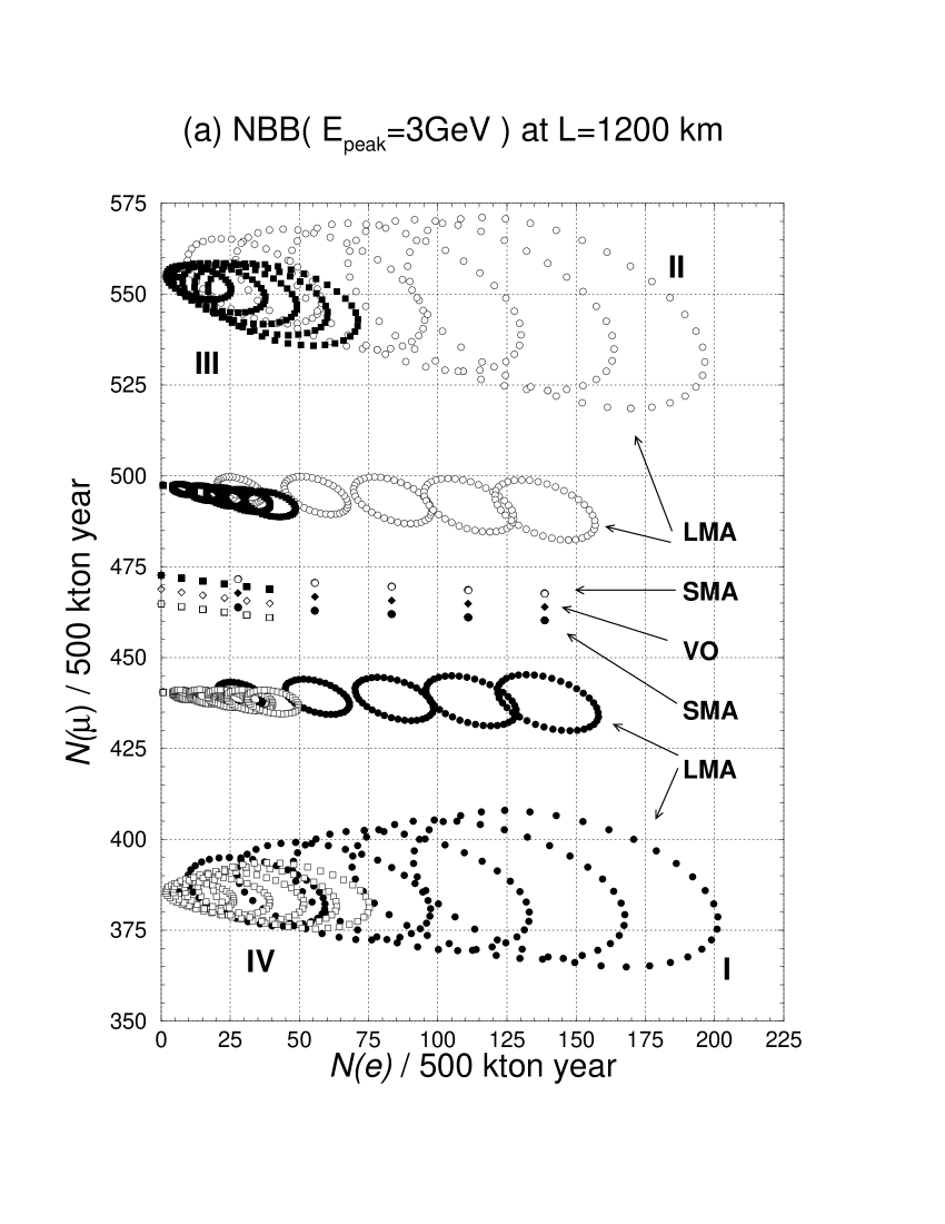
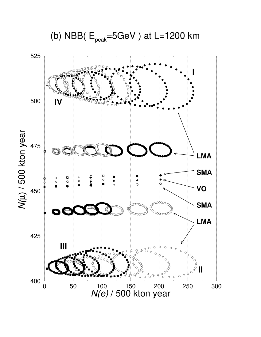
Figure 20: The neutrino parameter dependences of the expected numbers of $\nu_{e}$ CC events and $\nu_{\mu}$ CC events, $N(e)$ and $N(\mu)$, respectively, for the NBB with $E_{\rm peak}=3$ GeV (a) and 5 GeV (b) 500 kton$\cdot$year at $L=1,200$ km. All the symbols are the same as those in Fig. 13.

In Fig. 20, we show the expected numbers of signal events, $N(\mu)$ and $N(e)$, for the same set of NBB’s, (a) NBB ($E_{\rm peak}=3$GeV) and (b) NBB ($E_{\rm peak}=5$GeV), each with 500 kton$\cdot$year at $L=1,200$ km. The three-neutrino model parameters and the matter density used for calculating those numbers are the same as those used to generate Fig. 13 for $L=2,100$ km; see eq.(12) and eq.(4.3). All the symbols are the same as those adopted in Fig. 13. The dependences of $N(e)$ on the input $\sin^{2}2\theta_{{}_{\rm CHOOZ}}$ are the same as those found in Fig. 13; $N(e)$ decreases as input $\sin^{2}2\theta_{{}_{\rm CHOOZ}}$ is decreased from 0.1 to 0.08, 0.06, 0.04, 0.02 and 0. The solid-circle, open-circle, solid-square and open-square points show the predictions of the LMA and SMA scenarios with neutrino mass hierarchy I, II, III and IV, respectively. For each hierarchy, the five larger grand circles give the predictions of the LMA scenario with $\delta m^{2}_{{}_{\rm SOL}}=15\times 10^{-5}$ eV², and the smaller circles are for the LMA with $\delta m^{2}_{{}_{\rm SOL}}=5\times 10^{-5}$ eV². The VO predictions of the neutrino mass hierarchies I and II (III and IV) cannot be distinguished, and they are given by the solid (open)-diamonds. The difference in $N(\mu)$ is largest in the LMA scenarios with $\delta m^{2}_{{}_{\rm SOL}}=15\times 10^{-5}$ eV², for which the hierarchy III predicts about 40 $\%$ larger (20 $\%$ smaller) $N(\mu)$ than the predictions of the hierarchy I for the NBB with $E_{\rm peak}=3$ GeV (5 GeV). When we compare Fig. 20 for $L=1,200$ km with the corresponding Fig. 13 for $L=2,100$ km, we notice that the prediction for $N(e)$ in the hierarchy III are significantly larger for $L=1,200$ km than those for $L=2,100$ km. If it were only $N(e)$ in Fig. 20 that effectively discriminates the neutrino mass hierarchy, we should expect significant reduction of the hierarchy discriminating capability of the VLBL experiments at $L=1,200$ km.

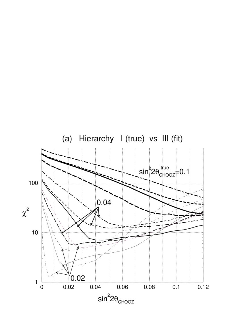
Figure 21: The same as Fig. 14(b) and Fig. 15(b), but for $L=1,200$ km.

In order to study these questions quantitatively, we repeat the $\chi^{2}$ fit for the following sets of experimental conditions ;

(4.34c)

(4.34f)

In Fig. 21 we show the minimum $\chi^{2}$ as functions of the fit parameter $\sin^{2}2\theta_{{}_{\rm CHOOZ}}$ for the data set (B’). The mean values of $N(\mu,E_{\rm peak})$ and $N(e,E_{\rm peak})$ at $L=1,200$ km and those at $L=295$ km are calculated for the experimental condition of eq.(4.34f) by assuming the LMA scenario and the hierarchy I, and by choosing 12 sets of the model parameters as in eq.(4.4.1); $\sin^{2}2\theta_{{}_{\rm CHOOZ}}^{true}=0.02$, 0.04, and 0.10 and $\delta_{{}_{\rm MNS}}^{true}=0^{\circ}$, 90^∘, 180^∘, and 270^∘. The $\chi^{2}$ fit has then been performed by assuming the LMA scenario with the hierarchy III; see eq.(4.4.1) for details. The 12 lines in Fig. 21(a) correspond to $\sin^{2}2\theta_{{}_{\rm CHOOZ}}^{true}=0.02$ (thin lines), 0.04 (medium-thick lines), 0.1 (thick lines) and $\delta_{{}_{\rm MNS}}^{true}=0^{\circ}$ (solid lines), $90^{\circ}$ (long-dashed lines), $180^{\circ}$ (short-dashed lines), $270^{\circ}$ (dot-dashed lines). We find that the neutrino mass hierarchy (between I and III) can be determined at $3\sigma$ level, for all four values of $\delta_{{}_{\rm MNS}}^{true}$ and when $\sin^{2}2\theta_{{}_{\rm CHOOZ}}=0.1$, and for $\delta_{{}_{\rm MNS}}^{true}=180^{\circ}$ and 270^∘ when $\sin^{2}2\theta_{{}_{\rm CHOOZ}}^{true}=0.04$. $\chi^{2}_{min}$ is greater than about 7 for $\delta_{{}_{\rm MNS}}^{true}=0^{\circ}$ and 90^∘ when $\sin^{2}2\theta_{{}_{\rm CHOOZ}}^{true}=0.04$. Even when $\sin^{2}2\theta_{{}_{\rm CHOOZ}}^{true}=0.02$, $\chi^{2}_{min}>4$ for $\delta_{{}_{\rm MNS}}^{true}=180^{\circ}$ and 270^∘. These results at $L=1,200$ km are not much worse than the results at $L=2,100$ km. We find that this is because the combination of the VLBL experiment and the $L=295$ km LBL experiment is still effective in distinguishing the hierarchy cases, even though the VLBL experiment at $L=1,200$ km itself cannot distinguish the hierarchy cases when $\sin^{2}2\theta_{{}_{\rm CHOOZ}}^{true}~{}{\hbox to0.0pt{\lower 3.5pt\hbox{$\mathchar 0\relax\sim$}\hss}\raise 1.0pt\hbox{$<$}}\,0.04$.

In Fig. 21 (b), the mean values of $N(\mu,E_{\rm peak})$ and $N(e,E_{\rm peak})$ are calculated for the 8 LMA points with hierarchy I; $\sin^{2}2\theta_{{}_{\rm CHOOZ}}=$0.06 and 0.10 for the four $\delta_{{}_{\rm MNS}}$ points in eq.(4.4.1). The $\chi^{2}$ fit has then been performed by assuming the SMA scenario within the hierarchy I; see eq.(4.4.2). The results of the fit are given for $\sin^{2}2\theta_{{}_{\rm CHOOZ}}^{true}$ = 0.06 (thin lines), 0.1 (thick lines) and $\delta_{{}_{\rm MNS}}^{true}$ = $0^{\circ}$ (solid lines), $90^{\circ}$ (long-dashed lines), $180^{\circ}$ (short-dashed lines), $270^{\circ}$ (dot-dashed lines). The qualitative features of the results shown in Fig. 21(b) are very similar to those of Fig. 15(b) at $L=2,100$ km. The VLBL experiment with HIPA do not seem to have the capability to distinguish the scenarios of the solar-neutrino oscillation models. This is mainly because the magnitude of oscillation phase $\Delta_{12}$ is smaller than 2.1 even for $\delta m^{2}_{{}_{\rm SOL}}=10\times 10^{-5}$eV² and $L/E_{\nu}=2,100$km/4GeV. We should rely on the results of the solar-neutrino oscillation measurements and the forthcoming reactor neutrino oscillation experiments [45].

Figure 22: The same as Fig. 18, but for $L=1,200$ km.

Fig. 22 shows the regions in the $\sin^{2}2\theta_{{}_{\rm CHOOZ}}$ v.s. $\delta_{{}_{\rm MNS}}$ plane which are allowed by the VLBL experiments at $L=2,100$ km with 500 kton$\cdot$year each for NBB ($E_{\rm peak}=5$GeV) and NBB ($E_{\rm peak}=3$GeV), and the LBL experiment at $L=295$ km with 100 kton$\cdot$year for NBB ($\langle p_{\pi}\rangle=2$GeV); eq.(4.34f). All the model parameters used to calculate the expected numbers of events and the symbols of the figures are the same as those adopted for Fig. 18. The four input points at $\delta_{{}_{\rm MNS}}^{true}=0^{\circ},90^{\circ},180^{\circ},270^{\circ}$ and $\sin^{2}2\theta_{{}_{\rm CHOOZ}}^{true}=0.06$ are shown by the solid-circle in each plane, and the region with $\chi^{2}_{min}<1$, 4, and 9 are shown by the solid, dashed, and dotted boundaries, respectably. The $\chi^{2}$ fit has been performed by assuming the LMA scenario with the hierarchy I, but otherwise by allowing all the model parameters to vary freely; see eq.(4.4.1).

The results shown in Fig. 22 look very similar to those of Fig. 18 for the combination of the VLBL experiment at $L=2,100$ km and the LBL experiment at $L=295$ km; eq.(4.29f). For $\delta_{{}_{\rm MNS}}^{true}=90^{\circ}$ and 270^∘, we cannot constrain the CP phase at all from these experiments. For $\delta_{{}_{\rm MNS}}^{true}=0^{\circ}$ and 180^∘, there appear a region of $\chi^{2}_{min}<1$ where $\delta_{{}_{\rm MNS}}$ is constrained, but the preferred region covers the whole range at $\chi^{2}_{min}<4$ level. We find that the area of the $\chi^{2}_{min}<1$ region is almost the same as that of the $L=2,100$ km experiment in Fig. 18 for each $\delta_{{}_{\rm MNS}}^{true}$ case. We conclude that the capability of measuring $\sin^{2}2\theta_{{}_{\rm CHOOZ}}$ and $\delta_{{}_{\rm MNS}}$ in the LMA scenario is very similar between the VLBL experiments at $L=2,100$ km and those at $L=1,200$ km.

		$\delta_{{}_{\rm MNS}}=0^{\circ}$	$90^{\circ}$	$180^{\circ}$	$270^{\circ}$
$\delta m^{2}_{{}_{\rm ATM}}$	(A’)	$3.50^{+0.065}_{-0.075}$	$3.50^{+0.075}_{-0.08}$	$3.50^{+0.07}_{-0.08}$	$3.50^{+0.085}_{-0.07}$
$(\times 10^{-3})$ (eV2)	(B’)	$3.50^{+0.065}_{-0.05}$	$3.50^{+0.065}_{-0.075}$	$3.50^{+0.07}_{-0.075}$	$3.50^{+0.07}_{-0.07}$
${\rm sin}^{2}2\theta_{{}_{\rm ATM}}$	(A’)	$>0.9940$	$>0.9940$	$>0.9935$	$>0.9935$
	(B’)	$>0.9945$	$>0.9945$	$>0.9945$	$>0.9945$

Table 9: The mean and the $1\sigma$ errors of $\delta m^{2}_{{}_{\rm ATM}}$ and the one-sigma level bound of $\sin^{2}2\theta_{{}_{\rm ATM}}^{true}$ when the input data are calculated for the four LMA points (eq.(4.4.1) at $\sin^{2}2\theta_{{}_{\rm CHOOZ}}^{true}$ = 0.06) and the fits are performed by assuming the LMA scenarios. (A’) Results with 500 kton$\cdot$year each for NBB($E_{\rm peak}=5$ GeV) and NBB($E_{\rm peak}=3$ GeV) at $L=1,200$ km. (B’) In addition, 100 kton$\cdot$year data from NBB($\langle p_{\pi}\rangle=2$ GeV) at $L=295$ km are included in the fit.

Finally, we show in Table 9 the expected accuracy of the measurements of $\delta m^{2}_{{}_{\rm ATM}}$ and $\sin^{2}2\theta_{{}_{\rm ATM}}$. The expected number of events are calculated for $\delta m^{2~{}true}_{{}_{\rm AMT}}=3.5\times 10^{-3}$eV² and $\sin^{2}2\theta_{{}_{\rm ATM}}^{true}=1.0$ in the LMA scenario with the hierarchy I. The 4 LMA input points and the fit parameters are the same as those used for Table 7. The mean and the one-sigma errors for fitted $\delta m^{2}_{{}_{\rm ATM}}$ and the one-sigma lower bound for $\sin^{2}2\theta_{{}_{\rm ATM}}$ are shown in the Table 9. The results of the VLBL experiment only, eq.(4.34c), are shown in the (A’) row, whereas those obtained by adding the LBL experiment at $L=295$ km, eq.(4.34f), are shown in the (B’) rows. By comparing the results of Table 7 and Table 9, we find that more precise measurements of $\delta m^{2}_{{}_{\rm ATM}}$ and $\sin^{2}2\theta_{{}_{\rm ATM}}$ can be achieved by the VLBL experiments at $L=1,200$ km. As mentioned above, this is essentially because the two NBB’s that we choose for studying the potential of the $L=1,200$ km experiments cover the two sides of the $P_{\nu_{\mu}\rightarrow\nu_{\mu}}=0$ node, whereas one of the two NBB’s chosen for studying the $L=2,100$ km case sits on top of the node to minimize $N(\mu)$. We find that the accuracy of $\delta m^{2}_{{}_{\rm ATM}}$ and $\sin^{2}2\theta_{{}_{\rm CHOOZ}}$ measurements at the $L=2,100$ km experiments can be improved, if a NBB with higher peak energy is added. Because higher $E_{\rm peak}$ NBB gives higher $\tau$-backgrounds and larger $N(\mu)$, the optimal choice of the beam-type and beam energy should be determined according to the prime physics objectives and the details of the proposed detectors.

5 Summary and discussions

The KEK-JAERI joint project on HIPA (High Intensity Proton Accelerator) [22] will start delivering $10^{21}$ POT (protons on target) at 50 GeV per one operation year by the year 2007. This compares with $3.85\times 10^{19}$ POT [47] at 12 GeV which are being provided by the KEK PS for the K2K neutrino oscillation experiment. The HIPA project thus provides us with an excellent opportunities of extending the K2K experiment, by shooting the neutrino beam from the HIPA to SK (the Super-Kamiokande) with $L=295$ km [19]. Refinement of the measurements of the atmospheric neutrino oscillation parameters ($\delta m^{2}_{{}_{\rm ATM}}$ and $\sin^{2}2\theta_{{}_{\rm ATM}}$) and the first measurement of the $\nu_{\mu}\rightarrow\nu_{e}$ oscillation parameter ($\sin^{2}2\theta_{{}_{\rm CHOOZ}}$) by observing the electron appearance are the main targets of the proposed experiment [19].

In this report, we explore the possibility of extending the LBL experiments to a much longer base-line length ($L>$ 1000 km) as a second stage of the neutrino oscillation experiments using the HIPA beam. In particular, we examine in detail the physics potential of VLBL experiments at $L=2,100$ km, which is approximately the distance between the HIPA and Beijing, where strong interests in constructing a huge neutrino detector (BAND) have been expressed [27]. We also examine the case at $L$ = 1,200 km carefully in order to study the sensitivity of physics outputs on the base-line lengths of the same order. The distance 1,200 km is approximately that between the HIPA and the central Korea, where strong interests in LBL neutrino oscillation experiments are expressed.

We study the physics potential of such VLBL experiments within the three-neutrino model. The three-neutrino model gives a consistent picture of all the neutrino oscillation observations except the LSND experiment, and has six parameters those are observables by neutrino-oscillation phenomena: two mass-squared differences, $\delta m^{2}_{12}=\pm\delta m_{{}_{\rm SOL}}^{2}$ and $\delta m^{2}_{13}=\pm\delta m_{{}_{\rm ATM}}^{2}$, three angles, $\sin^{2}2\theta_{{}_{\rm SOL}}$, $\sin^{2}2\theta_{{}_{\rm ATM}}$, and $\sin^{2}2\theta_{{}_{\rm CHOOZ}}$, and one phase, $\delta_{{}_{\rm MNS}}$. The main objectives of such VLBL experiments may be summarized by the following four questions :

1. Can we distinguish the neutrino mass hierarchy cases ?

2. Can we distinguish the solar neutrino oscillation scenarios ($\delta m^{2}_{{}_{\rm SOL}}$ and $\sin^{2}2\theta_{{}_{\rm SOL}}$) ?

3. Can we measure the two unknown parameters of the model, $\sin^{2}2\theta_{{}_{\rm CHOOZ}}$ and $\delta_{{}_{\rm MNS}}$ ?

4. How much can we improve the measurements of $\delta m^{2}_{{}_{\rm ATM}}$ and $\sin^{2}2\theta_{{}_{\rm ATM}}$ ?

In order to quantify our answers to the above questions, we make the following simplifications for the neutrino beams and the detector capability.

1. High-energy NBB’s with $E_{\rm peak}=3\sim 6$ GeV for the VLBL experiments.

2. Low-energy NBB with $\langle p_{\pi}\rangle$ = 2 GeV to represent the LBL experiment to SK.

3. 100 kton-level detector which is capable of detecting $\nu_{\mu}$ CC and $\nu_{e}$ CC events almost perfectly, but is not necessarily capable of measuring the particle charges and hadron energies.

4. Backgrounds from secondary beams and from leptonic $\tau$ decays of the $\nu_{\tau}$ CC events, as well as those from $\pi^{0}$-$e$ misidentification the neutral current processes are accounted for.

5. Common flux normalization errors of 3 $\%$ is assigned for the high-energy NBB’s, and an independent 3 $\%$ error for the low-energy NBB.

6. Overall uncertainty in the matter density is assumed to be 3.3 $\%$ for each experiment.

The detector capabilities of (iii) and (iv) are taken from those of the SK detector which may be common for water-$\check{\rm C}$erenkov detectors.

We find the following observations. By assuming that the HIPA-to-SK experiment measures the atmospheric-neutrino oscillation parameters to be centered at $\delta m^{2}_{{}_{\rm ATM}}=3.5\times 10^{-3}$ eV² and $\sin^{2}2\theta_{{}_{\rm ATM}}=1$, and by assuming that its cumulative effects can be represented by

(5.2)

we find that VLBL experiments of

$$\left.\begin{tabular}[]{l}500 kton$\cdot$year at $L=2,100$ km with NBB($E_{\rm peak}=6$ GeV)\\ 500 kton$\cdot$year at $L=2,100$ km with NBB($E_{\rm peak}=4$ GeV)\end{tabular}\right\}$$ (5.5)

can give the following answers :

1. If the neutrino mass hierarchy I is realized in Nature, then the hierarchy III can be rejected at $3\sigma$ ($1\sigma$) level if $\sin^{2}2\theta_{{}_{\rm CHOOZ}}>$ 0.04 (0.02). See Fig. 14 (b).

2. If the LMA scenario ($\delta m^{2}_{{}_{\rm SOL}}=10\times 10^{-4}$ eV², $\sin^{2}2\theta_{{}_{\rm SOL}}=0.8$) is realized in Nature, and if $\sin^{2}2\theta_{{}_{\rm CHOOZ}}>$0.06, the SMA/VO scenarios can be rejected at one-sigma level when $\delta_{{}_{\rm MNS}}$ is around $0^{\circ}$ or $180^{\circ}$ but not at all when $\delta_{{}_{\rm MNS}}$ is around $90^{\circ}$ or $270^{\circ}$. See Fig. 15 (b).

3. If the LMA scenario ($\delta m^{2}_{{}_{\rm SOL}}=10\times 10^{-5}$ eV², $\sin^{2}2\theta_{{}_{\rm SOL}}=0.8$) is realized in Nature, and if $\sin^{2}2\theta_{{}_{\rm CHOOZ}}=0.06$, then $0.04<\sin^{2}2\theta_{{}_{\rm CHOOZ}}<0.1$ is obtained when $\delta_{{}_{\rm MNS}}$ is around $0^{\circ}$ or $180^{\circ}$, $0.02<\sin^{2}2\theta_{{}_{\rm CHOOZ}}<0.08$ when $\delta_{{}_{\rm MNS}}$ is around $90^{\circ}$, $0.045<\sin^{2}2\theta_{{}_{\rm CHOOZ}}<0.12$ when $\delta_{{}_{\rm MNS}}$ is around $270^{\circ}$. $\delta_{{}_{\rm MNS}}$ can be constrained to local values at one-sigma level when the true $\delta_{{}_{\rm MNS}}$ is around $0^{\circ}$ or $180^{\circ}$ but it is unconstrained when it is around $90^{\circ}$ or $270^{\circ}$. See Fig. 18.

4. If the LMA scenario ($\delta m^{2}_{{}_{\rm SOL}}=10\times 10^{-4}$ eV², $\sin^{2}2\theta_{{}_{\rm SOL}}=0.8$) is realized in Nature, $\delta m^{2}_{{}_{\rm ATM}}$ is measured with the $3\%$ accuracy and $\sin^{2}2\theta_{{}_{\rm ATM}}$ to 1$\%$ level. See Table 7.

Summing up, a combination of LBL experiments at $L=295$ km and VLBL experiments at $L=2,100$ km with the NBB’s from HIPA can determine the neutrino mass hierarchy at $3\sigma$ level if $\sin^{2}2\theta_{{}_{\rm CHOOZ}}>$0.04, cannot distinguish the LMA scenario from the SMA/VO scenarios well, can constrain $\sin^{2}2\theta_{{}_{\rm CHOOZ}}$, and it can also constrain $\delta_{{}_{\rm MNS}}$ at one-sigma level in some cases. The errors of the atmospheric-neutrino oscillation parameters are reduced to $\delta(\delta m^{2}_{{}_{\rm ATM}})=\pm 0.1\times 10^{-3}$ eV² and $\sin^{2}2\theta_{{}_{\rm ATM}}>0.991$. Very similar results are found for a combination of $L=295$ km and $L=1,200$ km experiments. See Fig. 21, Fig. 22, and Table 9.

References

- [1] Kamiokande Collaboration, K.S. Hirata et al., Phys. Lett. B205, 416 (1988); ibid. B280, 146 (1992); Y. Fukuda et al., Phys. Lett. B335, 237 (1994); IMB Collaboration, D. Casper et al., Phys. Rev. Lett. 66, 2561 (1991); R. Becker-Szendy et al., Phys. Rev. D46, 3720 (1992); SOUDAN2 Collaboration, T. Kafka, Nucl. Phys. (Proc. Suppl.) B35, 427 (1994); M.C. Goodman, ibid. 38, (1995) 337; W.W.M. Allison et al., Phys. Lett. B391, 491 (1997); hep-ex/9901024.
- [2] The Super-Kamiokande Collaboration, Phys. Lett. B433, 9 (1998);Phys. Lett. B436, 33 (1998);Phys. Rev. Lett. 81, 1562 (1998).
- [3] S. Boyd, Nucl. Phys. Proc. Suppl. 98 175,(2001); Y. Oyama, hep-ex/0104014; T. Ishii, hep-ex/0106008; see also the K2K homepage, http://neutrino.kek.jp/index.html.
- [4] The CHOOZ Collaboration, Phys. Lett. B420, 397 (1998).
- [5] F. Boehm, et al., Phys. Rev. Lett. 84, 3764 (2000); Phys. Rev. D62, 072002 (2000); hep-ex/0107009.
- [6] The Super-Kamiokande Collaboration, Phys. Rev. Lett. 85, 3999 (2000); hep-ex/0105023; hep-ex/0106025.
- [7] Homestake Collaboration, B.T. Cleveland et al., Nucl. Phys. (Proc. Suppl.) B38, 47 (1995); Ap. J. 496, 505 (1998); Kamiokande Collaboration, Y. Suzuki, Nucl. Phys. (Proc. Suppl.) B38, 54 (1995); Y. Fukuda et al., Phys. Rev. Lett. 77, 1683 (1996); GALLEX Collaboration, W. Hampel et al., Phys. Lett. B388, 384 (1996); SAGE Collaboration, J.N. Abdurashitov et al., Phys. Rev. Lett. 77, 4708 (1996); Super-Kamiokande Collaboration, Y. Fukuda et al., Phys. Rev. Lett. 81, 1158 (1998); Phys. Rev. Lett. 82, 1810 (1999).
- [8] J.N. Bahcall, M.H. Pinsonneault, and S. Basu, Astrophys. J. 555 990 (2001); see also the homepage of J.N. Bahcall, http://www.sns.ias.edu/~jnb/.
- [9] The Super-Kamiokande Collaboration, Phys. Rev. Lett. 86, 5656 (2001); Phys. Rev. Lett. 86, 5651 (2001); hep-ex/0106064.
- [10] The SNO collaboration, Phys. Rev. Lett. 87, 071301 (2001); see also the SNO collaboration home page, http://www.sno.phy.queensu.ca/.
- [11] M. Nakagawa Z. Maki and S. Sakata, Prog. Theor. Phys. 28, 870 (1962).
- [12] L. Wolfenstein, Phys. Rev. D17, 2369 (1978).
- [13] S.P. Mikheyev and A.Yu. Smirnov, Yad. Fiz. 42, 1441 (1985), [Sov.J.Nucl.Phys.42, 913 (1986)]; Nuovo Cimento C9, 17 (1986).
- [14] B. Pontecorvo, Zh.Eksp. Teor. Fiz. 53, 1717 (1967); S.M. Bilenky and B. Pontecorvo, Phys. Rep. 41, 225 (1978); V. Barger, R.J.N. Phillips and K. Whisnant, Phys. Rev. D24, 538 (1981); S.L. Glashow and L.M. Krauss, Phys. Lett. B190, 199 (1987).
- [15] The LSND Collaboration, Phys. Rev. Lett. 77, 3082 (1996); Phys. Rev. Lett. 81, 1774 (1998); see also the LSND collaboration home page, http://www.neutrino.lanl.gov/LSND/; the KARMEN Collaboration, Phys. Rev. Lett. 81, 520 (1998); hep-ex/9809007; see also the KARMEN collaboration home page, http://www-ik1.fzk.de/www/karmen/karmen_e.html.
- [16] The MINOS collaboration home page, http://www-numi.fnal.gov:8875/.
- [17] The ICARUS Collaboration, hep-ex/9812006; hep-ex/0103008; see also the ICARUS collaboration home page, http://www.aquila.infn.it/icarus/.
- [18] A. Rubbia, Nucl. Phys. Proc. Suppl. 91 223 (2000); hep-ex/0008071; see also the OPERA collaboration home page, http://operaweb.web.cern.ch/operaweb/index.shtml.
- [19] The JHF Neutrino Working Group, hep-ex/0106019; see also the JHF Neutrino Working Group home page, http://neutrino.kek.jp/jhfnu/.
- [20] A. Bazarko, et al., Nucl. Phys. Proc. Suppl. 91, 210 (2000); hep-ex/0009056; see also the MiniBooNe collaboration home page, http://www-boone.fnal.gov/.
- [21] See e.g. , H. Minakata and H. Nunokawa, Phys. Rev. D57 4403 (1998); Phys. Lett. B413, 369 (1997); Phys. Lett. B495, 369 (2000); hep-ph/0009091; JHEP 0110 001 (2001); hep-ph/0111130; M. Koike and J. Sato, Phys. Rev. D62 073006 (2000); J. Sato, hep-ph/9910442; K. Dick, M. Freund, P. Huber, and M. Lindner, Nucl. Phys. B588, 101 (2000); Nucl. Phys. B598, 543 (2001); B. Richter, hep-ph/0008222; V. Barger, S. Geer, R. Raja, and K. Whisnant, Phys. Rev. D63 113011 (2001); V. Barger, et al., hep-ph/0103052; L. Wai, B. Patterson, hep-ph/0101090; J.J. Gomez-Cadenas, et al., hep-ph/0105297; Zhi-zhong Xing, Phys. Rev. D64 073014 (2001); Lian-You Shan, Bing-Lin Young, Xinmin Zhang, hep-ph/0110414.
- [22] See the HIPA home page, http://jkj.tokai.jaeri.go.jp/.
- [23] S. Geer, Phys. Rev. D57 6989 (1998); Erratum-ibid. D59 039903 (1999); hep-ph/9712290; V. Barger, S. Geer, and K. Whisnant, Phys. Rev. D61 053004 (2000); V. Barger, S. Geer, R. Raja, and K. Whisnant, Phys. Rev. D62 013004 (2000); Phys. Rev. D62 073002 (2000); Phys. Lett. B485, 379 (2000); Phys. Rev. D63 033002 (2001); S. Geer, hep-ph/0008155.
- [24] C. Albright, et al., hep-ex/0008064; M.L. Mangano, et al., hep-ph/0105155; J. Aysto, et al., hep-ph/0109217; A. De Roeck, J. Ellis, and F. Gianotti, hep-ex/0112004; T. Ota, J. Sato, and Y. Kuno, Phys. Lett. B520, 289 (2001).
- [25] See e.g., talk giving by Y. Kuno, at “International Workshop on Nuclear and Particle Physics at 50-GeV PS”, KEK, Japan, Dec.10-12, 2001, http://www-jhf.kek.jp/NP01/.
- [26] A part of this work has been reported by N. Okamura at BCP4, Ise, Japan, Feb.19-23, 2001; M. Aoki, K. Hagiwara, Y. Hayato, T. Kobayashi, T, Nakaya, K. Nishikawa and N. Okamura, hep-ph/0104220.
- [27] H. Chen, et al., hep-ph/0104266; Y.F. Wang, et al., hep-ph/0111317.
- [28] N. Cabibbo, Phys. Rev. Lett. 10, 531 (1964); M. Kobayashi and T. Maskawa Prog. Theor. Phys. 49, 652 (1973).
- [29] K. Hagiwara and N. Okamura, Nucl. Phys. B548, 60 (1999).
- [30] C. Jarlskog, Phys. Rev. Lett. 55, 1039 (1985); Z. Phys. C29, 491 (1985).
- [31] See e.g. , talk giving by M. Messier, at “The 3rd Workshop on Neutrino Oscillations and their Origin (NOON2001)”, ICRR, Univ. of Tokyo, Kashiwa, Japan, Dec.5-8, 2001, http://www-sk.icrr.u-tokyo.ac.jp/noon2001/.
- [32] H. Minakata, Phys. Lett. B356, 61 (1995); hep-ph/9612259; O. Yasuda and H. Minakata, hep-ph/9602386; O. Yasuda Phys. Rev. D58 0901301 (1998); G.L. Fogli, E. Lisi, D. Montanino, and A. Palazzo, Phys. Rev. D61 073009 (2000); G.L. Fogli, E. Lisi, A. Marrone, D. Montanio and A. Palazzo, hep-ph/0104221; John N. Bahcall, M.C. Gonzalez-Garcia, C. Pena-Garay, hep-ph/0111150; M.C. Gonzalez-Garcia, M. Maltoni, C. Pena-Garay, and J.W.F. Valle, Phys. Rev. D63 033005 (2001).
- [33] K.S. Hirata, et al., Phys. Rev. Lett. 58, 1490 (1987);Phys. Rev. D38, 448 (1988); R.M. Bionta, et al., Phys. Rev. Lett. 58, 1494 (1987); H. Minakata and H. Nunokawa, Phys. Lett. B504, 301 (2001); M. Kachelriess, A. Stumia, R. Tomas and J.W.F. Valle, hep-ph/0108100; M. Kachelriess, R. Tomas and J.W.F. Valle, JHEP 0101 030 (2001).
- [34] See e.g. , P.H. Frampton and S.L. Glashow, Phys. Lett. B461, 95 (1999); L. Hall, H. Murayama, and N. Weiner, Phys. Rev. Lett. 84, 2572 (2000); E.Kh. Akhmedov, G.C. Branco, and M.N. Rebelo, Phys. Lett. B478, 215 (2000); D. Black, A.H. Fariborz, S. Nasri, J. Schechter, Phys. Rev. D62 073015 (2000); N. Haba, Y. Matsui, N. Okamura, and T. Suzuki, Phys. Lett. B489, 184 (2000); T. Miura, T. Shindou, E. Takasugi, and M. Yoshimura, Phys. Rev. D63 053006 (2001); L. Lavoura, Phys. Rev. D62 093011 (2000); B. Stech, Phys. Rev. D62 093019 (2000); Y. Koide and A. Ghosal, Phys. Lett. B488, 344 (2000); N. Okamura and M. Tanimoto, Prog. Theor. Phys. 105, 459 (2001); T. Miura, E. Takasugi, and M. Yoshimura,Prog. Theor. Phys. 104, 1173 (2000); H.B. Nielsen and Y. Takanishi, Nucl. Phys. B604, 281 (2001); C.H. Albright and S.M. Barr, Phys. Rev. D64 073010 (2001); H. Fritzsch, Z.Z. Xing, Phys. Lett. B517, 363 (2001).
- [35] See e.g. , J. Arafune and J. Sato, Phys. Rev. DD55 1653 (1997); J. Arafune, M. Koike, and J. Sato, Phys. Rev. D56 3093 (1997); Erratum-ibid. D601199051999; M. Koike and J. Sato, Mod. Phys. Lett. A14 1297 (1999); T. Ota and J. Sato, Phys. Rev. D63 093004 (2001); T. Miura, T. Shindou, E. Takasugi, and M. Yoshimura, Phys. Rev. D64 013002 (2001);Phys. Rev. D64 073017 (2001).
- [36] Y. Yamanoi et al., “Large Horn Magnets at the KEK Neutrino Beam Line”, KEK Preprint 97-225, November 1997.
- [37] D. Beavis, et al., BNL E-889 proposal.
- [38] T.Kobayashi for the JHF Neutrino Working Group, talk given at the Fifth KEK Topical Conference, KEK, Tsukuba, Japan, Novemver (2001).
- [39] R.Brun, F.Carminati, “GEANT Detector Description and Simulation Tool”, CERN Program Library Long Write-up W5013, September 1993.
- [40] C. Zeitnitz and T.A. Gabriel, “The GEANT-CALOR interface and benchmark calculations for ZEUS calorimeters”, NIM A349 (1994) 106-111; T.A. Gabriel, J.D. Amburgey and B.L. Bishop, “Calor: A Monte Carlo Program Package For The Design And Analysis Of Calorimeter Systems”, ORNL/TM-5619; C. Zeitnitz and T.A. Gabriel, “The GEANT-CALOR interface and benchmark calculations for ZEUS calorimeters”, NIM A349 (1994) 106-111.
- [41] See the home page, http://neutrino.kek.jp/JHF-VLBL/flux/.
- [42] See e.g. , K. Ishihara, Ph.D. thesis, ICRR-Report-457-2000-1; Y. Hayato, talk at NuInt01, KEK, December 13-16, to appear in the proceedings.
- [43] Particle Data Group, Eur. Phys. J. C15, 1 (2000).
- [44] See the home page of the Borexino collaboration, http://almime.mi.infn.it/.
-
[45]
see the KamLAND collaboration home page,
http://www.awa.tohoku.ac.jp/html/KamLAND/index.html. - [46] M. Aoki, K. Hagiwara and N. Okamura, (in preparation).
- [47] C.K. Jung for the K2K Collaboration, talk given at XX International Symposium on Lepton and Photon Interactions at High Energies, Rome, Italy, July (2001).