OCHA-PP-184

hep-ph/0112336

PACS: 11.25.Mj

1 Introduction

The idea of dynamical generation of extra dimension [1] has been applied to, for example, grand unified theories [2], electroweak symmetry breaking [3], and supersymmetry breaking [4], etc. From the high energy point of view, the extra dimension is generated dynamically at low-energy scale as a consequence of a certain fermion condensation mechanism [1]. On the other hand, from the low-energy point of view, it seems that the space-time dimension will disappear above the ultraviolet cut-off scale, or, in other words, the asymptotic disappearance of space-time (ADST) occurs. In ref. [5], the condensation mechanism is naively applied to the gauge theory in D dimensions, as well as the gravity theory in 3 dimensions. A characteristic feature of the generated (D+1) gauge theory or 4D gravity by this mechanism is that the generated dimension is discretized by an interval $a$. Application to gravity and the non-commutative geometry is further developed [7, 8].

In this paper, we study the effective 4D gauge theory in which one spatial dimension is dynamically generated from the 3D action [5]. We restrict our study to QED which is a simplest and well tested gauge theory. In general, due to the discretized spatial dimension, introduction of chiral fermions into the gauge theory causes so called “doubling problem” [9, 10]. Since there is no chiral fermion in QED, we are not troubled by this problem. This is another reason why we focus on QED in our study. The appearance of the discretized extra dimension modifies the interactions between the photon and the electron. We first summarize the Feynman rules in the model and show that the modification occurs associated with the direction of the extra dimension and the interval parameter $a$. It is explicitly shown that the usual QED in 4D is restored in the continuum limit of the lattice in the extra dimension. It is, therefore, worth examining how large the size of $a$ is allowed phenomenologically. We study the annihilation process $e^{+}e^{-}\to\gamma\gamma$ as a distinctive example of the QED process, and find quantitative constraint on the parameter $a$ from the measurement of the total cross section of the process at LEP2 experiments. The experimental data [11] tells us that the current constraint on the parameter $a$ is at most a few hundred GeV. We show that the future $e^{+}e^{-}$ linear collider may give a further bound on the parameter $a$ around TeV scale.

In the next section, we briefly review the mechanism of dynamical generation of the extra dimension. The effective 4D QED generated from the 3D action based on the mechanism is also studied. In Sec. 3, the annihilation process $e^{+}e^{-}\to\gamma\gamma$ is studied in the light of the measurement at LEP2. The last section is devoted to summary.

2 QED with the dynamical generation of extra dimension

2.1 The dynamical generation of extra dimension

We briefly review how 4D gauge theory is derived from the 3D action following refs. [1, 5]. First let us consider the following 3 dimensional gauge theory: It consists of $N$ sets of the gauge groups $G$’s labelled by $G(n),G(n+1),\cdots$, located at integer sites $n,n+1,\cdots$, and $G_{s}$’s labelled by $G_{s}(n+\frac{1}{2}),G(n+\frac{3}{2}),\cdots$, located at half-integer sites $n+1/2,n+3/2,\cdots$. The gauge coupling constants of $G$’s and $G_{s}$’s are $g$ and $g_{s}$, respectively. The Weyl fermion $\chi(m,\ell)$ belongs to a fundamental representation of $G_{(s)}(m)$ at the site $m$, and an anti-fundamental representation of $G_{(s)}(\ell)$ at the site $\ell$. The sites $m$ and $\ell$ always differ by $\frac{1}{2}$, so that the fermion $\chi$ connects the neighboring $G$ and $G_{s}$. In the following, we fix $G={\rm SU}(m)$ and $G_{s}={\rm SU}(n_{s})$ for definiteness. We depict the diagrammatic description of the model in Fig. 1. The outgoing fermion from $G(n)$, $\chi(n,n+\frac{1}{2})$, is in the fundamental representation of SU($m$) at the site $n$ and the anti-fundamental representation of SU($n_{s}$) at $n+\frac{1}{2}$. On the other hand, the outgoing fermion from $G_{s}(n+\frac{1}{2})$, $\chi(n+\frac{1}{2},n)$, is in the fundamental and the anti-fundamental representations of SU($n_{s}$) at $n+\frac{1}{2}$ and SU($m$) at $n+1$, respectively.

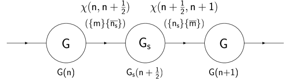
Figure 1: Diagrammatic description of the representation of the fermion $\chi$ under the two neighboring gauge groups, $G={\rm SU}(m)$ and $G_{s}={\rm SU}(n_{s})$. The outgoing fermion $\chi(n,n+\frac{1}{2})$ from $G(n)$ is in the fundamental and the anti-fundamental representations of SU($m$) at the site $n$ and SU($n_{s}$) at the site $n+\frac{1}{2}$, respectively. On the other hand, the outgoing fermion $\chi(n+\frac{1}{2},n)$ from $G_{s}(n+\frac{1}{2})$ is in the fundamental and the anti-fundamental representations of SU($n_{s}$) at the site $n+\frac{1}{2}$ and SU($m$) at the site $n+1$, respectively.

The gauge coupling $g_{s}$ becomes strong below a certain low energy scale of $\Lambda_{s}$ and, as a result, it leads to the fermion condensations whose vacuum expectation values are given by the $m\times m$ unitary matrix $U$:

$$\frac{1}{2\pi(f_{s})^{2}}\langle\chi(n,n+\frac{1}{2})\chi(n+\frac{1}{2},n+1)\rangle \equiv U(x;n,n+1),$$ (2.1)

where $f_{s}$ is the decay constant. Now $U(x;n,n+1)$ plays the role of a link field between $G(n)$ and $G(n+1)$. We identify the set of discrete points connected linearly by the link fields to the extra dimension. Then, the low-energy effective action below $\Lambda_{s}$ is given as follows

$$S_{\rm eff} = -\frac{1}{2(g_{3})^{2}}\int d^{3}x~{}~{}a\sum_{n=1}^{N}~{}~{}{\rm Tr}(F_{ij}(x,n)F^{ij}(x,n))$$ (2.2)

$$+ f_{s}\int d^{3}x~{}\sum^{N}_{n=1}{\rm Tr}\left[\left(D_{i}U(x;n,n+1)\right)^{\dagger}\left(D^{i}U(x;n,n+1)\right)\right],$$

where $i,j=0,1,2$. The first line of (2.2) is the action of 3D gauge field, while the second line is the action for the dynamically generated link field $U(x;n,n+1)$. The covariant derivative in (2.2) is defined by

$$D_{i} \equiv \partial_{i}+iA_{i}(x,n)U(x;n,n+1)-iU(x;n,n+1)A_{i}(x,n+1).$$ (2.3)

It is easy to see that eq.(2.2) is essentially the 4D action for the gauge field of $G$, where the third spatial dimension is discretized. By noting $U(x;n,n+1)=e^{iaA_{3}(x:n)}$ and expanding eq.(2.2) in a small dimensionful parameter $a$, the action could be written as

$$S_{\rm eff} = -\frac{1}{2(g_{3+1})^{2}}\int d^{3}x~{}~{}a\sum_{n=1}^{N}~{}~{}{\rm Tr}(F_{\mu\nu}(x,n)F^{\mu\nu}(x,n))$$ (2.4)

$$~{}~{}+\mbox{(higher order terms in $a$)},$$

where $\mu,\nu=0\sim 3$, and the 4D gauge coupling $g_{3+1}$ is given in terms of the 3D coupling $g_{3}$ as

$$(g_{3+1})^{2} = a(g_{3})^{2},~{}~{}~{}~{}a=\frac{1}{g_{3}(f_{s})^{1/2}}.$$ (2.5)

2.2 Effective 4D QED

Let us write down the effective 4D QED having the dynamically generated extra spatial dimension following Sec. 2.1. The action for the gauge kinetic term, $S_{g}$, is already shown in the previous subsection for SU(n) gauge group (see, eq. (2.4)). In the case of QED, $S_{g}$ is written as

$$S_{g}=-\frac{1}{4}\int d^{3}x~{}~{}a\sum_{n=1}^{N}F_{\mu\nu}(x,n)F^{\mu\nu}(x,n).$$ (2.6)

The gauge invariant action $S_{f}$ for the fermion $\psi$ in 3D is given as;

$$S_{f} = \int d^{3}x\sum_{n=1}^{N}\Bigl{(}2aK\bar{\psi}(x,n)i\gamma^{i}D_{i}(A(n))\psi(x,n)-\bar{\psi}(x,n)\psi(x,n)\Bigr{)},$$ (2.7)

where $i,j=0,1,2$ and we introduce the hopping parameter $K$ instead of the fermion mass parameter. The covariant derivative in (2.7) is defined by

$$D_{i} \equiv \partial_{i}+ieA_{i}.$$ (2.8)

After the fermion condensation occurs as in eq. (2.1), the link field $U(x;n,n+1)$ connects two fermions at the different sites $n$ and $n+1$. Then, the following pieces are also gauge invariant in addition to (2.7);

$$\Delta_{1}S_{f} = \int d^{3}x\sum_{n=1}^{N}K\Bigl{(}\bar{\psi}(n)i\gamma^{3}U(n,n+1)\psi(n+1)$$ (2.9a)

$$~{}~{}~{}~{}~{}~{}~{}-\bar{\psi}(n+1)i\gamma^{3}U(n,n+1)^{\dagger}\psi(n)\Bigr{)},$$

$$\Delta_{2}S_{f} = \int d^{3}x\sum_{n=1}^{N}K\Bigl{(}\bar{\psi}(n)U(n,n+1)\psi(n+1)$$ (2.9b)

$$~{}~{}~{}~{}~{}~{}~{}+\bar{\psi}(n+1)U(n,n+1)^{\dagger}\psi(n)\Bigr{)},$$

Here, we give a comment on the relative weight of these two terms, following Wilson in ref. [9]. If we choose the effective action as $\Delta_{1}S_{f}+c\Delta_{2}S_{f}$ with a relative weight $c$, then the dispersion relation of the electron becomes

$$E^{2}-\left(\frac{\sin p_{3}a}{a}\right)^{2}-\left(\frac{1-2Kc\cos p_{3}a}{2aK}\right)^{2}=0,$$ (2.10)

where we have set $p_{1}=p_{2}=0$ for simplicity. Using the variable $x$ defined by $x=\cos p_{3}a$, the dispersion relation is generally the second order algebraic equation, namely,

$$(c^{2}-1)x^{2}-\left(\frac{c}{K}\right)x+1+\left(\frac{1}{2K}\right)^{2}-(aE)^{2}=0.$$ (2.11)

Therefore, when $c^{2}\neq 1$, we have generally two different solutions for the dispersion relation of electron for each spin degree of freedom. Then, we have too many degrees of freedom for electron. To avoid this difficulty, we have to choose $c=1$ or $-1$ and make the dispersion relation to be the first order algebraic equation for $x$. We have, therefore, adopted $c=1$ in the above effective actions. This comment suggests that the condensation mechanism to generate the effective actions is so arranged that it may satisfy this condition.

Identifying the link filed $U$ as the third spatial component of the photon field

$$U(x;n,n+1)=e^{iaeA_{3}(x:n)},$$ (2.12)

we obtain the effective 4D QED action for small $a$, having a discretized spatial dimension with the interval $a$.

2.3 Feynman rules

The Feynman rules of the effective QED with a discretized spatial dimension could be found from the actions (2.6), (2.7) and (2.2). Because of the discretized spatial dimension, the Lorentz invariance is manifestly violated for the finite size of $a$ so that the interaction between photon and electron becomes different from the usual QED.

• Photon propagator
  The photon propagator is given by (2.6). Taking account of the discrete dimension, the derivative of the gauge field associated with the third spatial axis should be replaced by the corresponding different operator. Then, the propagator is given as

  $$D_{\mu\nu}(k) = \frac{-ig_{\mu\nu}}{\displaystyle{\sum_{i=0,1,2}k_{i}k^{i}-\left(\frac{2}{a}\right)^{2}\sin^{2}\left(\frac{k_{3}a}{2}\right)}}$$ (2.13a)

  $$\equiv \frac{-ig_{\mu\nu}}{\widetilde{k}_{\mu}^{*}\widetilde{k}^{\mu}},$$ (2.13b)

  where the second term of the denominator in (2.13a) reflects the latticized dimension. The use of the notation

  $$\widetilde{k}_{\mu} = \left(\widetilde{k}_{0},\widetilde{k}_{1},\widetilde{k}_{2},\widetilde{k}_{3}\right)$$ (2.14)

  $$= \left(k_{0},k_{1},k_{2},\frac{2}{a}e^{-\frac{i}{2}k_{3}a}\sin\left(\frac{k_{3}a}{2}\right)\right),$$

  allows us to have the familiar form of the photon propagator (2.13b).

• Electron propagator
  We find the electron propagator from eqs. (2.7) and (2.2), by rescaling the fermion fields canonically. The discrete dimension gives

  $$iS_{F}^{-1}(p) = \gamma^{i}p_{i}+\gamma^{3}\frac{\sin\left(p_{3}a\right)}{a}-\frac{1}{2aK}\left\{(1-2K\cos(p_{3}a)\right\}$$ (2.15a)

  $$= \ooalign{\hfil/\hfil\crcr$\widetilde{p}$}-m,$$ (2.15d)

  where

  $$\widetilde{p}_{\mu} = \left(\widetilde{p}_{0},\widetilde{p}_{1},\widetilde{p}_{2},\widetilde{p}_{3}\right)$$ (2.16a)

  $$= \left(p_{0},p_{1},p_{2},\frac{\sin(p_{3}a)}{a}\right),$$

  $$m \equiv \frac{1}{2aK}\left\{(1-2K\cos(p_{3}a)\right\}.$$ (2.16b)

  Note that the third component of the electron momentum $\widetilde{p}_{3}$ has a different form from the photon momentum $\widetilde{k}_{3}$ in eq. (2.14).

• electron-electron-photon vertex
  The $ee\gamma$ vertex is modified associated with the non-canonical form in the third component of the momentum. The momentum dependent vertex function at the tree level is given by

  $$\Gamma^{\mu} = \left\{\gamma^{i},\gamma^{3}\frac{1}{2}\left(e^{-ip_{3}a}+e^{+i(p_{3}+k_{3})a}\right)-\frac{i}{2}\left(e^{-ip_{3}a}-e^{+i(p_{3}+k_{3})a}\right)\right\},$$ (2.17)

  where $p$ and $k$ are the incoming electron and photon momenta, respectively. The outgoing electron momentum is $p+k$.

• Photon polarization sum and the spin sum of the spinors
  It is rather straightforward to find the rules of the polarization sum of the photon and the spin sum of the spinors. They could be derived from the total action in the usual manner. The photon polarization sum follows

  $$\sum_{\lambda=1,2}\epsilon_{\mu}(\lambda)\epsilon_{\nu}^{*}(\lambda) = -g_{\mu\nu}-\frac{\widetilde{k}_{\mu}\widetilde{k}_{\nu}^{*}}{\left|\widetilde{k}\cdot n\right|^{2}}+\frac{n_{\mu}\widetilde{k}_{\nu}^{*}}{\left(\widetilde{k}\cdot n\right)^{*}}+\frac{\left(n_{\nu}\widetilde{k}_{\mu}^{*}\right)^{*}}{\widetilde{k}\cdot n},$$ (2.18)

  where $n=(1,0,0,0)$. The spin sum of the spinors are given by

  $$\sum_{{\rm spin}}u(p)\overline{u}(p) = \ooalign{\hfil/\hfil\crcr$\widetilde{p}$}+m,$$ (2.19c)

  $$\sum_{{\rm spin}}v(p)\overline{v}(p) = \ooalign{\hfil/\hfil\crcr$\widetilde{p}$}-m.$$ (2.19f)

• Ward identity
  The momentum dependence of the $ee\gamma$ vertex (2.17) gives rise to a somewhat different form of the Ward identity. Taking account of the complex parameter $\widetilde{k}_{\mu}$ as the “momentum” of the photon, we find that there are two expressions of the Ward identity corresponding to the incoming and the outgoing photons:

  $$-i\widetilde{k}_{\mu}\Gamma^{\mu} = S_{F}^{-1}(p+k)-S_{F}^{-1}(p),$$ (2.20a)

  $$+i\widetilde{k}^{*}_{\mu}\Gamma^{\mu} = S_{F}^{-1}(p-k)-S_{F}^{-1}(p),$$ (2.20b)

  where (2.20a) and (2.20b) correspond to the vertices shown in Fig. 2(a) and 2(b), respectively. Owing to these Ward identities, we understand that the effective 4D QED having dynamically generated spatial dimension is manifestly gauge invariant, even though it violates the Lorentz invariance.

  

  Figure 2: The $ee\gamma$ vertices corresponding to the Ward identities in eq. (2.20a) (a) and in eq. (2.20b) (b).

3 $e^{+}e^{-}\to\gamma\gamma$ in the effective 4D QED

In this section, we study the annihilation process $e^{+}e^{-}\to\gamma\gamma$ taking account of the discrete third spatial dimension generated in the effective 4D QED. The axis $x^{3}$ representing this discrete dimension may be considered to be fixed in a special frame where the cosmic microwave background radiation is isotropic. Then, the beam axis of the $e^{+}e^{-}$ collider is generally tilted from the $x^{3}$ axis by an angle $\chi$. Since the earth moves and rotates in this special frame for the cosmic background radiation, the angle $\chi$ changes in time. The main time variation of $\chi$ comes from the daily rotation of the earth (see [12] for the more detailed treatment on this problem). In this paper we estimate the total cross section averaged over the angle $\chi$ which can be compared with the ordinary total cross section measured by summing up the events obtained during the running time of the machine (several months or years). To clarify the day-night effect and the seasonal effect of the differential cross section of our process is an interesting problem to be pursued. Another possibility is that the discrete dimension is randomly directed at any place. Without referring to the details of the nature of the discrete dimension, that is, whether it is fixed in the special frame or is randomly directed, the averaging of the cross section over the tilt angle is a way to take into account the existence of the discrete dimension properly.

As is shown in the previous section, the usual 4D QED is restored in the continuum limit of the third spatial dimension, or the $a\to 0$ limit. It is interesting, however, to examine how the cross section of the process is modified for the finite size of the interval parameter $a$, since $a$ is small but non-vanishing in the effective 4D QED. The presence of the finite $a$ leads to the explicit violation of the Lorentz invariance in 4D, but the evidence of the Lorentz symmetry violation has not been found yet. Therefore, we have to restrict our study to a small non-vanishing $a$. Furthermore, we take the massless electron limit for simplicity. In this limit, the gauge invariance requires the elimination of the part of the $ee\gamma$ vertex function (2.17) not proportional to $\gamma_{3}$. Then, the Ward identity of the massless case is available in the original form (• ‣ 2.3). For the incoming photon with the momentum $k$, the vertex function in the massless limit is given by

$$\Gamma^{\mu} = \left\{\gamma^{i},\gamma^{3}\frac{1}{2}\left(e^{-ip_{3}a}+e^{+i(p_{3}+k_{3})a}\right)\right\}.$$ (3.1)

As is similar to the usual QED, there are $t$- and $u$-channel diagrams in the process $e^{+}e^{-}\to\gamma\gamma$. The Feynman diagrams for both channels are shown in Fig. 3.

Figure 3: Feynman diagrams for the annihilation process $e^{+}e^{-}\to\gamma\gamma$. The $t$-channel and the $u$-channel diagrams are shown in (a) and (b), respectively.

The total amplitude is given by

$$iM = \left(M^{\mu\nu}(t)+M^{\mu\nu}(u)\right)\epsilon^{*}_{\mu}(p^{\prime})\epsilon^{*}_{\nu}(k^{\prime}),$$ (3.2)

where $M^{\mu\nu}(t)$ and $M^{\mu\nu}(u)$ are the $t$- and $u$-channel amplitudes without the photon polarization vectors, respectively, and are found to be

$$M^{\mu\nu}(t) \equiv -e^{2}\overline{v}(\widetilde{p})\Gamma^{\mu}S_{F}(k-k^{\prime})\Gamma^{\nu}u(\widetilde{k}),$$ (3.3a)

$$M^{\mu\nu}(u) \equiv -e^{2}\overline{v}(\widetilde{p})\Gamma^{\nu}S_{F}(k-p^{\prime})\Gamma^{\mu}u(\widetilde{k}).$$ (3.3b)

From the gauge invariance, the following relations hold as in the usual QED when we employ $\widetilde{p}^{\prime}$ and $\widetilde{k}^{\prime}$ as the photon “momentum”

$$\widetilde{p}^{\prime*}_{\mu}\left(M^{\mu\nu}(t)+M^{\mu\nu}(u)\right) = \widetilde{k}^{\prime*}_{\nu}\left(M^{\mu\nu}(t)+M^{\mu\nu}(u)\right)=0.$$ (3.4)

In practice, we take a small $a$ limit. Namely, we expand the photon momentum (2.14), the electron momentum (2.16a) and the $ee\gamma$ vertex function (3.1) in the parameter $a$, and consistently drop the higher order terms in the amplitudes.

Figure 4: Momentum assignment of the process $e^{+}e^{-}\to\gamma\gamma$ in the CM system, where $x^{3}$ is the discrete dimension and the beam axis is tilted from the $x^{3}$ axis by the angle $\chi$. The scattering angle of the process is denoted by $\theta_{*}$. The parameters $A$ and $B$ account for the change of the dispersion relation in this model. The explicit forms of them are given in eq. (3).

As is shown previously, the dispersion relations between the energy and the momentum for photon and electron take the different forms due to the finite interval parameter $a$. This tells us that the assignment of the four momenta in a specific frame is affected by the finite $a$-parameter. In Fig. 4, we show explicitly the momentum configuration of the relevant particles in the CM system. The four momenta receive the following corrections due to the finite $a$-parameter:

$$k = \frac{\sqrt{s}}{2}(1,As_{\chi},0,Ac_{\chi}),$$ (3.5a)

$$p = \frac{\sqrt{s}}{2}(1,-As_{\chi},0,-Ac_{\chi}),$$ (3.5b)

$$k^{\prime} = \frac{\sqrt{s}}{2}(1,Bs_{\theta}c_{\phi},Bs_{\theta}c_{\phi},Bc_{\theta}),$$ (3.5c)

$$p^{\prime} = \frac{\sqrt{s}}{2}(1,-Bs_{\theta}c_{\phi},-Bs_{\theta}s_{\phi},-Bc_{\theta}),$$ (3.5d)

where $A$ and $B$ are defined as

$$A(\chi) \equiv 1+\frac{sa^{2}}{24}\cos^{4}\chi,$$ (3.6a)

$$B(\theta) \equiv 1+\frac{1}{4}\frac{sa^{2}}{24}\cos^{4}\theta.$$ (3.6b)

Then, the squared amplitude is given by

$$\sum|M|^{2} = 8e^{4}\left(\frac{1+\omega}{1-\omega}+\frac{1-\omega}{1+\omega}\right)$$ (3.7)

$$+ 8e^{4}\frac{sa^{2}}{12}\left[\frac{1}{(1-\omega)^{2}}(c_{\chi}-c_{\theta})^{4}+\frac{3}{4}(2c_{\chi}-c_{\theta})^{2}\right.$$

$$~{}~{}~{}~{}~{}-\frac{1}{1-\omega}\left\{c_{\chi}^{3}(c_{\chi}+c_{\theta})-c_{\theta}(c_{\chi}-c_{\theta})^{3}+\frac{3}{2}(2c_{\chi}-c_{\theta})^{2}(1-c_{\chi}c_{\theta})\right\}$$

$$~{}~{}~{}~{}~{}+\frac{1}{(1+\omega)^{2}}(c_{\chi}+c_{\theta})^{4}+\frac{3}{4}(2c_{\chi}+c_{\theta})^{2}$$

$$~{}~{}~{}~{}~{}\left.-\frac{1}{1+\omega}\left\{c_{\chi}^{3}(c_{\chi}-c_{\theta})+c_{\theta}(c_{\chi}+c_{\theta})^{3}+\frac{3}{2}(2c_{\chi}+c_{\theta})^{2}(1+c_{\chi}c_{\theta})\right\}\right.$$

$$~{}~{}~{}~{}~{}\left.+\frac{1}{(1-\omega)(1+\omega)}3c_{\theta}^{4}\right],$$

where we summed over the spin of incoming electron and positron, and the polarization of outgoing photons. In the above expression, $\omega$ is defined as $\omega\equiv\cos\theta_{*}$ with the scattering angle $\theta_{*}$ of the process given in Fig. 4. The first line in r.h.s. is consistent with the usual QED, while the other lines correspond to the correction terms due to the latticized dimension. The second and third lines are found from the $t$-channel diagram, and the forth and fifth lines are from the $u$-channel diagram, while the last line represents the interference of the two diagrams, which must be absent in the usual QED. In the usual QED, it is well known that the squared amplitude of the $u$-channel diagram in the CM system is obtained from that of the $t$-channel diagram, by replacing the scattering angle $\omega=\cos\theta_{*}$ by $-\omega=-\cos\theta_{*}$ (see, the first line in (3.7)). We find similarly that the correction terms of the $u$-channel (forth and fifth lines) are obtained from those of the $t$-channel (second and third lines) by the replacement $\theta\to\theta+\pi$, or $\chi\to\chi+\pi$. Either replacement induces $\omega\to-\omega$, since we have $\omega=c_{\theta_{*}}=c_{\chi}c_{\theta}+s_{\chi}s_{\theta}c_{\phi}$. The finite $a$ corrections appear also in the beam flux factor and in the phase space integration in the CM system. The beam flux $f$ depends on the relative velocity of the electron and the positron, namely

$$f=sv_{\rm rel}=2s|v_{\rm electron}|.$$ (3.8)

The velocity $v$ defined by $\mbox{\boldmath{$v$}}=\partial E/\partial\mbox{\boldmath{$p$}}$, depends on the modified dispersion relation of electron or positron, and so we have

$$\frac{1}{f}=\frac{1}{2s}A^{3},$$ (3.9)

which is valid in the lowest order corrections in $a$. The phase space integration $d\Phi$ is also modified as

$$d\Phi=\frac{1}{16\pi}B^{5}d(\cos\theta)\frac{d\phi}{2\pi},$$ (3.10)

in the same lowest order approximation.

Now, the differential cross section of the process $e^{+}e^{-}\to\gamma\gamma$ in the CM system are given by

$$d\sigma(e^{+}e^{-}\to\gamma\gamma)=\frac{1}{64\pi s}A(\chi)^{3}B(\theta)^{5}d(\cos\theta)\frac{d\phi}{2\pi}\frac{1}{4}\sum|M|^{2}.$$ (3.11)

The factor $\frac{1}{64\pi s}$ in the above formula is the product of $\frac{1}{2s}$ from eq. (3.9), $\frac{1}{16\pi}$ from eq. (3.10), and the Bose factor $\frac{1}{2}$ coming from the final two photons. Here, we will take the average of the differential cross section over the angle $\chi$. For this purpose, it is convenient to move to another coordinate frame in which the beam axis of the incident electron points to the direction of the new $x^{3}_{*}$ axis and the scattering angle $\theta_{*}$ and $\phi_{*}$ are the polar angle and the azimuthal angle of the new coordinate frame. Then, the $\chi$ dependence disappears in the denominators made of $1\pm\omega=1\pm c_{\theta_{*}}$, and the $\chi$ dependence appears only in the numerators. Now, the average over $\chi$ is easily performed, by using the transformation rule $c_{\theta}=c_{\chi}c_{\theta_{*}}-s_{\chi}s_{\theta_{*}}c_{\phi_{*}}$ and the following formulas of the average:

$$\langle c_{\chi}^{4}\rangle=\langle s_{\chi}^{4}\rangle=\frac{3}{8},~{}\langle c_{\chi}^{2}s_{\chi}^{2}\rangle=\frac{1}{8},~{}\langle c_{\chi}^{2}\rangle=\langle s_{\chi}^{2}\rangle=\frac{1}{2}.$$ (3.12)

After taking the average over $\chi$ is finished, the integration over the azimuthal angle $\phi_{*}$ is easily performed.

Then, the total cross section averaged over the tilt angle $\chi$ of the process $e^{+}e^{-}\to\gamma\gamma$ in the CM system are obtained as (note $\omega\equiv\cos\theta_{*}$)

$$\sigma = \frac{\pi\alpha^{2}}{s}\int d\omega\left\{\frac{1+\omega^{2}}{1-\omega^{2}}\right.$$ (3.13)

$$+ \frac{sa^{2}}{24}\times\left[\frac{3}{16}\left(3+\frac{5}{32}(3+2\omega^{2}+3\omega^{4})\right)\times\left(\frac{1+\omega}{1-\omega}+\frac{1-\omega}{1+\omega}\right)\right.$$

$$+ \frac{3}{32}(55+7\omega^{2})$$

$$+ \frac{1}{1-\omega}\frac{1}{64}(237-438\omega+210\omega^{2}-54\omega^{3}+9\omega^{4})$$

$$+ \frac{1}{1+\omega}\frac{1}{64}(237+438\omega+210\omega^{2}+54\omega^{3}+9\omega^{4})$$

$$+ \left.\left.\frac{9}{64}\frac{8\omega^{2}+3(1-\omega^{2})^{2}}{1-\omega^{2}}\right]\right\}.$$

Figure 5: The upper bound of the interval parameter $a$ as a function of $\sqrt{s}$, obtained from the total cross section of the process $e^{+}e^{-}\to\gamma\gamma$. We assume that the cross section normalized by the QED prediction can be measured in the 5% accuracy. The bottom horizontal line denotes the constraint on $a^{-1}$ from the LEP2 experiments. The middle horizontal line is the expected lower bound on $a^{-1}$ at $500{\rm GeV}$ $e^{+}e^{-}$ linear collider, while the top horizontal line corresponds to the bound on $a^{-1}$ at $1{\rm TeV}$ $e^{+}e^{-}$ linear collider.

The total cross section of $e^{+}e^{-}\to\gamma\gamma$ has been measured at LEP2 [11], in which the experiment has been done for the scattering angle $|\cos\theta_{*}|<0.9$. We find the total cross section within this range of $\cos\theta_{*}$ as

$$\frac{\sigma}{\sigma_{\rm QED}} \approx 1+0.30sa^{2},$$ (3.14)

where the cross section in QED is given by

$$\sigma_{\rm QED} = \frac{\pi\alpha^{2}}{s}\int d\omega\frac{1+\omega^{2}}{1-\omega^{2}}$$ (3.15)

$$= 4.09\frac{\pi\alpha^{2}}{s}.$$

In ref. [11], the total cross section is measured at $\sqrt{s}=189{\rm GeV}$. When the measured total cross section is normalized by the QED prediction, the error is about $5\%$ [11]. Then it constrains the parameter $a$ as

$$0.30sa^{2} \mathchar 0\relax\sim < 0.05~{}~{}~{}\mbox{\rm for $\sqrt{s}=189{\rm GeV}$}$$ (3.16)

$$\Longrightarrow 1/a\,{\hbox to0.0pt{\lower 3.5pt\hbox{$\mathchar 0\relax\sim$}\hss}\raise 1.0pt\hbox{$>$}}\,461{\rm GeV}.$$

From its dimensionality, the parameter $a$ always appears as a product with the CM energy ($\sqrt{s}$) and the correction to the physical observables appears in ${\cal O}(sa^{2})$. This is because $a\to-a$ means the parity transformation $p_{3}\to-p_{3}$ which is kept invariant in this effective 4D QED. Then, the constraint on the $a$-parameter will be much stronger than (3.16) as the beam energy increases if the cross section is measured as precisely as the LEP2 experiment [11]. We show in Fig. 5 the parameter $a^{-1}$ in the unit of GeV as a function of the beam energy $\sqrt{s}({\rm GeV})$. In the figure, we assume that the experimental error of the total cross section normalized by the QED prediction is $5\%$. The bottom horizontal line in the figure corresponds to the lower bound on $a^{-1}$ from the LEP2 experiment performed at $\sqrt{s}=189{\rm GeV}$, eq.(3.16). As is mentioned, the lower bound on $a^{-1}$ significantly increases for the higher $\sqrt{s}$. We show the middle and the top horizontal lines as the expected constraints on $a^{-1}$ from the future $e^{+}e^{-}$ linear collider at $\sqrt{s}=500{\rm GeV}$ and $1{\rm TeV}$, respectively. The constraint on the parameter $a$ is found to be $1/a\,{\hbox to0.0pt{\lower 3.5pt\hbox{$\mathchar 0\relax\sim$}\hss}\raise 1.0pt\hbox{$>$}}\,1.2{\rm TeV}$ at the $500{\rm GeV}$ linear collider, while the $1{\rm TeV}$ linear collider will cover the $a$ parameter less than $(2.4{\rm TeV})^{-1}$.

4 Summary

We have studied the 4D QED in which the third spatial dimension is dynamically generated owing to the mechanism of the certain fermion-pair condensation proposed in ref. [1]. The direct consequence of employing this mechanism is that the dynamically generated extra dimension is discretized by the interval parameter $a$. We have derived the effective 4D QED action explicitly, and shown the Feynman rules. They take different forms from those in the usual QED due to the latticized fourth dimension. Taking account of the discrete third spatial dimension, we examined the QED process $e^{+}e^{-}\to\gamma\gamma$ and found the quantitative constraint on the interval parameter $a$ from the LEP2 experiment. In our estimation of the cross section of $e^{+}e^{-}\to\gamma\gamma$, the beam axis of $e^{+}$ and $e^{-}$ is considered to be tilted from the discrete third spatial dimension, and the cross section is averaged over the tilt angle. This averaging is a way to take into account the existence of the discrete dimension properly, without referring the details of the nature of the discrete dimension, that is, whether the discrete dimension is fixed in the special frame for the microwave background radiation, or the direction of it is randomly generated. Then, the constraint on the interval parameter is found to be $1/a\,{\hbox to0.0pt{\lower 3.5pt\hbox{$\mathchar 0\relax\sim$}\hss}\raise 1.0pt\hbox{$>$}}\,461{\rm GeV}$, and the constraint will be stronger at future $e^{+}e^{-}$ linear collider. If the linear collider could measure the total cross section of the process as accurately as in LEP2, the size of the lattice in the third spatial dimension will be bound as: $1/a\,{\hbox to0.0pt{\lower 3.5pt\hbox{$\mathchar 0\relax\sim$}\hss}\raise 1.0pt\hbox{$>$}}\,1.2{\rm TeV}$ for $\sqrt{s}=500{\rm GeV}$ and $1/a\,{\hbox to0.0pt{\lower 3.5pt\hbox{$\mathchar 0\relax\sim$}\hss}\raise 1.0pt\hbox{$>$}}\,2.4{\rm TeV}$ for $\sqrt{s}=1{\rm TeV}$.

The finite size of $a$ modifies the dispersion relation, which indicates the violation of the Lorentz invariance. The possibility of violating the Lorentz symmetry has been examined, and two phenomena difficult to explain in modern astrophysics, such as the ultra high-energy cosmic rays beyond the GZK cut-off of $10^{20}{\rm eV}$, and $20{\rm TeV}$ $\gamma$-ray from the active galaxy of Markarian 501, may be understood by the Lorentz symmetry violation [13]. The interpretation of these problems in the framework of our model will be done elsewhere [14].

References

- [1] N. Arkani-Hamed, A. G. Cohen and H. Georgi, Phys. Rev. Lett. 86, 4757 (2001).
-
[2]
C. Csaki, G. D. Kribs and J. Terning,
Phys. Rev. D 65, 015004 (2002);
H. C. Cheng, K. T. Matchev and J. Wang, Phys. Lett. B 521, 308 (2001);
P. H. Chankowski, A. Falkowski and S. Pokorski, JHEP 0208, 003 (2002). -
[3]
N. Arkani-Hamed, A. G. Cohen and H. Georgi,
Phys. Lett. B 513, 232 (2001);
H. J. He, C. T. Hill and T. M. Tait, Phys. Rev. D 65, 055006 (2002). -
[4]
C. Csaki, J. Erlich, C. Grojean and G. D. Kribs,
Phys. Rev. D 65, 015003 (2002);
H. C. Cheng, D. E. Kaplan, M. Schmaltz and W. Skiba, Phys. Lett. B 515, 395 (2001);
T. Kobayashi, N. Maru and K. Yoshioka, hep-ph/0110117. - [5] A. Sugamoto, Prog. Theor. Phys. 107, 793 (2002).
- [6] C. T. Hill, S. Pokorski and J. Wang, Phys. Rev. D 64, 105005 (2001).
- [7] M. Bander, Phys. Rev. D 64, 105021 (2001).
- [8] M. Alishahiha, Phys. Lett. B 517, 406 (2001).
- [9] K. G. Wilson, ”Quarks and Strings on a Lattice”, Erice Lecture Notes, 1975, CLNS-321 (1975).
- [10] H. B. Nielsen and M. Ninomiya, Phys. Lett. B 105, 219 (1981).
- [11] G. Abbiendi et al. [OPAL Collaboration], Phys. Lett. B 465, 303 (1999).
- [12] J. Kamoshita, OCHA-PP-191, June (2002) (hep-ph/0206223).
-
[13]
S. R. Coleman and S. L. Glashow,
Phys. Rev. D 59, 116008 (1999);
G. Amelino-Camelia and T. Piran, Phys. Rev. D 64, 036005 (2001);
L. Gonzalez-Mestres, AIP Conf. Proc. 558, 878 (2001);
O. Bertolami, Gen. Rel. Grav. 34, 707 (2002);
R. J. Protheroe and H. Meyer, Phys. Lett. B 493, 1 (2000);
T. Kifune, Astrophys. J. 518, L21 (1999);
H. Sato, astro-ph/0005218. - [14] G.C. Cho, E. Izumi, A. Sugamoto and I. Watanabe, in preparation.