hep-ph/0112334
                                                                         December, 2001

Determination of $\tan\beta$ at a Future $e^{+}e^{-}$ Linear Collider ^†
J. Gunion¹, T. Han², J. Jiang³, S. Mrenna⁴, A. Sopczak^5
1Davis Institute for HEP, U. of California, Davis, CA
²Dept. of Physics, U. of Wisconsin, Madison, WI
³Argonne National Laboratory, Chicago, IL
⁴Fermilab, Batavia, IL
⁵Lancaster University, UK

Abstract

It is widely stated that the ratio of neutral Higgs field vacuum expectation values, $\tan\beta$, is one of the most difficult parameters to determine in either the Minimal Supersymmetric Standard Model (MSSM) or a general type-II Two-Higgs Doublet Model (2HDM). Assuming an energy and integrated luminosity of $\sqrt{s}=500~{}{\rm GeV}$ and ${\cal L}=2000~{}{\rm fb}^{-1}$, we show that a very accurate determination of $\tan\beta$ will often be possible using Higgs production rates and/or Higgs decays. Based on a TESLA simulation, and assuming no other light Higgs bosons and $100\leq m_{A}\leq 200~{}{\rm GeV}$, we find that the rate for the process $e^{+}e^{-}\rightarrow b\overline{b}A\rightarrow b\overline{b}b\overline{b}$ provides an excellent determination of $\tan\beta$ at high $\tan\beta$. In the MSSM Higgs sector, the rate for $e^{+}e^{-}\rightarrow b\overline{b}A+b\overline{b}H\rightarrow b\overline{b}b\overline{b}$ ($e^{+}e^{-}\rightarrow HA\rightarrow b\overline{b}b\overline{b}$) provides a good determination of $\tan\beta$ at high (low) $\tan\beta$, respectively, at moderate $m_{A}$ values. We also show that direct measurement of the average total width of the $H$ and $A$ in $e^{+}e^{-}\rightarrow HA\rightarrow b\overline{b}b\overline{b}$ events provides an excellent determination of $\tan\beta$ at large $\tan\beta$.

Contribution to the Snowmass 2001 Workshop on “The Future of Particle Physics”, Snowmass, CO, USA, July 2001

Abstract

It is widely stated that the ratio of neutral Higgs field vacuum expectation values, $\tan\beta$, is one of the most difficult parameters to determine in either the Minimal Supersymmetric Standard Model (MSSM) or a general type-II Two-Higgs Doublet Model (2HDM). Assuming an energy and integrated luminosity of $\sqrt{s}=500~{}{\rm GeV}$ and ${\cal L}=2000~{}{\rm fb}^{-1}$, we show that a very accurate determination of $\tan\beta$ will often be possible using Higgs production rates and/or Higgs decays. Based on a TESLA simulation, and assuming no other light Higgs bosons and $100\leq m_{A}\leq 200~{}{\rm GeV}$, we find that the rate for the process $e^{+}e^{-}\rightarrow b\overline{b}A\rightarrow b\overline{b}b\overline{b}$ provides an excellent determination of $\tan\beta$ at high $\tan\beta$. In the MSSM Higgs sector, the rate for $e^{+}e^{-}\rightarrow b\overline{b}A+b\overline{b}H\rightarrow b\overline{b}b\overline{b}$ ($e^{+}e^{-}\rightarrow HA\rightarrow b\overline{b}b\overline{b}$) provides a good determination of $\tan\beta$ at high (low) $\tan\beta$, respectively, at moderate $m_{A}$ values. We also show that direct measurement of the average total width of the $H$ and $A$ in $e^{+}e^{-}\rightarrow HA\rightarrow b\overline{b}b\overline{b}$ events provides an excellent determination of $\tan\beta$ at large $\tan\beta$.

I Introduction

A future linear collider has great potential for discovering new particles and measuring their properties. Theories beyond the Standard Model (SM) that resolve the hierarchy and fine-tuning problems typically involve extensions of its single-doublet Higgs sector to at least a two-doublet Higgs sector (2HDM). The most attractive such model is the MSSM, which contains a constrained two-Higgs-doublet sector. In other cases, the effective theory below some energy scale is equivalent to a 2HDM extension of the SM with no other new physics. While many parameters of theories beyond the SM can be measured with high precision, it is often stated that determination of the important parameter $\tan\beta=\langle H_{u}^{0}\rangle/\langle H_{d}^{0}\rangle$ (where $\langle H_{u}^{0}\rangle$ and $\langle H_{d}^{0}\rangle$ are responsible for up-type quark masses and down-type quark and lepton masses, respectively) is difficult, especially for large $\tan\beta$. However, Higgs boson couplings are very sensitive to $\tan\beta$. In particular, for a CP-conserving Higgs sector we have the following couplings [2] (at tree-level):

$$A\rightarrow b\overline{b}\propto\tan\beta;\quad A\rightarrow t\overline{t}\propto\cot\beta;\quad H^{+}\rightarrow t\overline{b}\propto m_{b}(1+\gamma_{5})\tan\beta+m_{t}(1-\gamma_{5})\cot\beta$$

$$h\rightarrow b\overline{b}\propto-{\sin\alpha\over\cos\beta};\quad h\rightarrow t\overline{t}\propto{\cos\alpha\over\sin\beta};\quad H\rightarrow b\overline{b}\propto{\cos\alpha\over\cos\beta};\quad H\rightarrow t\overline{t}\propto{\sin\alpha\over\sin\beta}\,,$$ (1)

where $\alpha$ is the mixing angle in the CP-even sector.

In this report, we show how various Higgs boson measurements can be used to determine $\tan\beta$, especially when $\tan\beta$ is large. Our focus will be on $b\overline{b}$+Higgs production, Higgs pair production in the $b\overline{b}b\overline{b}$ final state and Higgs total widths as measured in the pair production channel.

II The $b\overline{b}A\rightarrow b\overline{b}b\overline{b}$ bremsstrahlung process

The challenge of this study is the low expected production rate and the large irreducible background for a four-jet final state, as discussed in a previous study [3]. Searches for $b\bar{b}A$ and $b\bar{b}h$ were performed in this four-jet channel using LEP data taken at the $Z$ resonance [4, 5, 6, 7]. A LC analysis has been performed using event generators for the signal process $e^{+}e^{-}\rightarrow b\overline{b}A\rightarrow b\overline{b}b\overline{b}$ [8] and the $e^{+}e^{-}\rightarrow eW\nu,~{}e^{+}e^{-}Z,~{}WW,~{}ZZ,~{}q\overline{q}~{}(q=u,d,s,c,b),~{}t\overline{t},~{}hA$ background processes [9] that include initial-state radiation and beamstrahlung.

For a 100 GeV pseudoscalar Higgs boson and $\tan\beta=50$, the signal cross section is about 2 fb [10, 11, 12]. The generated events were passed through the fast detector simulation SGV [13]. The detector properties closely follow the TESLA detector Conceptual Design Report [14]. The simulation of the $b$-tagging performance is very important for this analysis. The efficiency versus purity distribution for the simulated b-tagging performance is shown in Fig. 1 for the hadronic event sample $e^{+}e^{-}\rightarrow q\bar{q}$ for 5 flavors, where efficiency is the ratio of simulated $b\overline{b}$ events after the selection to all simulated $b\overline{b}$ events, and purity is the ratio of simulated $b\overline{b}$ events after the selection to all selected $q\overline{q}$ events. Details of the event selection and background reduction are described elsewhere [3].

Figure 1: $b$-tagging performance.

For $m_{A}=100~{}{\rm GeV}$ in the context of the MSSM, the SM-like Higgs boson is the $H$ while the light $h$ is decoupled from $WW,ZZ$ [$\cos(\beta-\alpha)\sim 1$ and $\sin(\beta-\alpha)\sim 0$]. The $b\overline{b}h$ coupling is essentially equal (in magnitude) to the $b\overline{b}A$ coupling ($\propto\tan\beta$ at the tree level) and $m_{h}\sim m_{A}$, implying that it would not be possible to separate these two signals. Also important will be $hA$ production, which is $\propto\cos(\beta-\alpha)$ and will have full strength in this particular situation; $HA$ production will be strongly suppressed. We focus first on $b\overline{b}A\rightarrow b\overline{b}b\overline{b}$.

The expected background rate for a given $b\overline{b}A\rightarrow b\overline{b}b\overline{b}$ signal efficiency is shown in Fig. 2. One component of the background is $hA\rightarrow b\overline{b}b\overline{b}$; our selection procedures are, in part, designed to reduce this piece of the background as much as possible (e.g. by removing events with $m_{b\overline{b}}\sim m_{h}$ for the second $b\overline{b}$ pair). Nonetheless, it may lead to significant systematic error in the determination of $\tan\beta$ (see below). For the $b\overline{b}A\rightarrow b\overline{b}b\overline{b}$ signal, the sensitivity ${\rm S}/\sqrt{{\rm B}}$ for $m_{A}=100~{}{\rm GeV}$ is almost independent of the working point choice of signal efficiency in the range $\epsilon_{\rm sel}=5$% to 50%. For a working point choice of 10% efficiency, the total simulated background of about 16 million events is reduced to 100 background events with an equal number of signal events at $\tan\beta=50$. If this were the only contributing process, the resulting error on $\tan\beta=50$ would be 7%: $\Delta\tan^{2}\beta/\tan^{2}\beta=\Delta{\rm S}/{\rm S}=\sqrt{{\rm S}+{\rm B}}/{\rm S}=0.14.$ For smaller values of $\tan\beta$, the sensitivity decreases rapidly. A $5\sigma$ signal detection is still possible for $\tan\beta=35$. In the MSSM context, the $b\overline{b}h$ signal would essentially double the number of signal events and have exactly the same $\tan\beta$ dependence, yielding $\Delta\tan^{2}\beta/\tan^{2}\beta\sim\sqrt{300}/200\sim 0.085$ for $\tan\beta=50$.

Although the number of $hA$ background events is very small compared to the other background reactions after the event selection, interference between the signal $b\overline{b}A\rightarrow b\overline{b}b\overline{b}$ (plus $b\overline{b}h\rightarrow b\overline{b}b\overline{b}$) and the background $hA\rightarrow b\overline{b}b\overline{b}$ reaction could be important. At the working point, and after applying the selection procedures, the expected rate for the latter is $2\pm 1$ events for ${\cal L}=500~{}{\rm fb}^{-1}$. Let us momentarily retain only the $b\overline{b}A$ signal in discussing the interference. We first calculate the cross sections $\sigma(e^{+}e^{-}\rightarrow b\overline{b}A\rightarrow b\overline{b}b\overline{b})$, $\sigma(e^{+}e^{-}\rightarrow hA\rightarrow b\overline{b}b\overline{b})$, and $\sigma(e^{+}e^{-}\rightarrow b\overline{b}A+hA\rightarrow b\overline{b}b\overline{b})$ with CompHEP [15] before selections and define the interference as $\sigma_{\rm interf}=\sigma_{b\overline{b}A+hA}-\sigma_{b\overline{b}A}-\sigma_{hA}$. For the default value $m_{b}=4.62$ GeV, at $\tan\beta=50$ we obtain $\sigma_{b\overline{b}A}=1.83\pm 0.01$ fb, $\sigma_{hA}=36.85\pm 0.10$ fb, $\sigma_{b\overline{b}A+hA}=39.23\pm 0.12$ fb, $\sigma_{\rm interf}=0.55\pm 0.16$ fb. We observe a constructive interference similar in size to the signal. Thus, more signal events are expected than simulated and the statistical error estimate is conservative. After selection cuts, we have found 100 signal events vs. 2 $hA$ background events. The maximum interference magnitude arises if the interference events are signal-like yielding an interference excess of $(10+\sqrt{2})^{2}-100-2\sim 28$, a percentage ($\sim 30\%$) similar to the ratio obtained before selection cuts. If the events from the interference are background-like, the resulting systematic error will be small, since the $hA$ background is only a small part of the total background. Of course, in the MSSM context we have an exact prediction as a function of $\tan\beta$ for the combined contribution of $hA\rightarrow b\overline{b}b\overline{b}$ and $b\overline{b}A\rightarrow b\overline{b}b\overline{b}$ (plus $b\overline{b}h\rightarrow b\overline{b}b\overline{b}$), including all interferences, and this exact prediction can be compared to the data. In order to test this exact prediction, it may be helpful to compare theory and experiment for several different event selection procedures, including ones that give more emphasis to the $hA$ process. Of course, this exact prediction depends somewhat on other MSSM parameters, especially if decays of the $h$ or $H$ to pairs of supersymmetric particles are allowed or ratios of certain MSSM parameters are relatively large [16]. If this type of uncertainty exists, the systematic error on $\tan\beta$ can still be controlled by simultaneously simulating all sources of $b\overline{b}b\overline{b}$ events for various $\tan\beta$ values and fitting the complete data set (assuming that the MSSM parameters are known sufficiently well). Another possible theoretical systematic uncertainty derives from higher-order corrections. The full NLO QCD corrections are given in [17, 18]. There it is found that using the running $b$-quark mass incorporates the bulk of the NLO corrections. For example, for $m_{A}=100~{}{\rm GeV}$, employing $m_{b}(100~{}{\rm GeV})\sim 2.92~{}{\rm GeV}$ vs. $m_{b}(m_{b})\sim 4.62~{}{\rm GeV}$ yields (before cuts) a cross section of $\sim 0.75~{}{\rm fb}$ vs. $\sim 2~{}{\rm fb}$, respectively, at $\tan\beta=50$. The signal rates and resulting errors quoted in this section are those computed using $m_{b}=4.62~{}{\rm GeV}$. Use of the running mass would reduce the event rates and increase our error estimates; the resulting errors will be given in the MSSM context in our final figure. Higher-order corrections of all kinds will be even better known by the time the Linear Collider (LC) is constructed and data is taken and thus should not be a significant source of systematic uncertainty. The final source of systematic uncertainty is that associated with knowing the exact efficiency of the event selection procedure. At the working point of $\epsilon_{\rm sel}=10\%$, to achieve $\Delta\tan\beta/\tan\beta<0.05$ requires $\Delta\epsilon_{\rm sel}/\epsilon_{\rm sel}<0.1$, equivalent to $\Delta\epsilon_{\rm sel}<1\%$. This is probably the best that can be done.

Figure 2: Plots for $\sqrt{s}=500~{}{\rm GeV}$ and $b\overline{b}A$ events only, before including running of the $b$-quark mass. Left: Final background rate vs. signal efficiency for $m_{A}=100~{}{\rm GeV}$ and ${\cal L}=500~{}{\rm fb}^{-1}$. Right: Corresponding $\tan\beta$ statistical error for ${\cal L}=2000~{}{\rm fb}^{-1}$ and $m_{A}=100,150,200~{}{\rm GeV}$.

In addition to the $hA$ Higgs boson background, two other Higgs boson processes could lead to a $b\overline{b}b\overline{b}$ topology. First, the process $e^{+}e^{-}\rightarrow HZ$ can give a $b\overline{b}b\overline{b}$ final state. In fact, for large $\tan\beta$ the $HZ$ cross section is maximal and similar in size to the $hA$ cross section. Nonetheless, its contribution to the background is much smaller because the $HZ\rightarrow b\overline{b}b\overline{b}$ branching is below 10% compared to about 80% for $hA\rightarrow b\overline{b}b\overline{b}$. Since the $hA$ process contributed only 2% of the total background, the contribution to the background from the $HZ$ process can be neglected. The second Higgs boson process leading to a $b\overline{b}b\overline{b}$ topology is that already discussed, $e^{+}e^{-}\rightarrow b\overline{b}h$. The only distinction between this and the $e^{+}e^{-}\rightarrow b\overline{b}A$ process is a small difference in the angular distribution due to the different production matrix elements. Thus, the selection efficiency is almost identical. The production rate of the $b\overline{b}A$ process is proportional to $\tan^{2}\beta$ while the $b\overline{b}h$ production rate is proportional to $\sin^{2}\alpha/\cos^{2}\beta$. In the MSSM context, this latter factor is $\sim\tan^{2}\beta$ for $m_{A}=100~{}{\rm GeV}$ and large $\tan\beta$ (assuming $M_{\rm SUSY}\sim 1~{}{\rm TeV}$). In the general 2HDM, since $\tan\beta\approx 1/\cos\beta$ at large $\tan\beta$, the expected rate depends mostly on $\sin\alpha$ and the $h$ mass. In this more general case, if $m_{h}\approx m_{A}$ but the MSSM expectation of $\alpha\sim-\beta\sim-\pi/2$ does not hold, the enhancement of the $b\overline{b}A$ signal by the $b\overline{b}h$ addition would only allow a determination of $|\sin\alpha|$ as a function of the presumed value of $\tan\beta$ (using the constraint that one must obtain the observed number of $b\overline{b}h+b\overline{b}A$ events). Independent measurements of the $HZ$ and $hA$ production rates would then be needed to determine the value of $\beta-\alpha$ and only then could $\alpha$ and $\beta$ be measured separately.

It is estimated that ${\cal L}=2000~{}{\rm fb}^{-1}$ can be accumulated after several years of data-taking at the LC. Such high total luminosity is of particular importance for the $\tan\beta$ determination. In Fig. 2 we show the expected statistical error on $\tan\beta$ for $m_{A}=100,150$ and 200 GeV, assuming that the only measured process is $b\overline{b}A$. At the two higher $m_{A}$ values, in the MSSM context it is the $H$ that would be decoupled and have mass $m_{H}\sim m_{A}$ and the $h$ would be SM-like. Consequently, the $b\overline{b}H$ rate would be essentially identical to the $b\overline{b}A$ rate and, assuming that one could verify the MSSM Higgs context by independent means, would lead to still smaller $\tan\beta$ statistical errors than plotted, the exact decrease depending upon the signal to background ratio. For $m_{A}=150$ and $200~{}{\rm GeV}$, the $HA$ process (like the $hA$ process at $m_{A}=100~{}{\rm GeV}$) would have to be computed in a specific model context or its relative weight fitted by studying $b\overline{b}b\overline{b}$ production in greater detail in order to minimize any systematic error from this source.

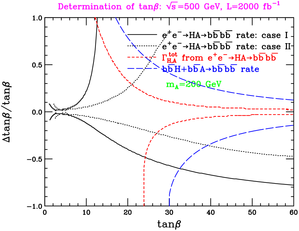
Figure 3: For the MSSM with $m_{A}=200$ GeV, and assuming ${\cal L}=2000~{}{\rm fb}^{-1}$ at $\sqrt{s}=500~{}{\rm GeV}$, we plot the $1\sigma$ statistical error band in $\Delta\tan\beta/\tan\beta$ as a function of $\tan\beta$ based on: (a) the rate for $e^{+}e^{-}\rightarrow b\overline{b}A+b\overline{b}H\rightarrow b\overline{b}b\overline{b}$ (with the $HA$ pair process reduced by the event selection); (b) the rate for $e^{+}e^{-}\rightarrow HA\rightarrow b\overline{b}b\overline{b}$; (c) the average of $\Gamma_{\rm tot}^{H}$ and $\Gamma_{\rm tot}^{A}$ as determined in $e^{+}e^{-}\rightarrow HA\rightarrow b\overline{b}b\overline{b}$ events. Results for (a), (b) and (c) all include running $b$-quark mass effects and employ HDECAY [19].

III Complementary Methods: $H,A$ branching ratios and total widths

Owing to the large variation of the $H$, $A$ and $H^{\pm}$ branching fractions to various allowed modes for low to moderate $\tan\beta$ in the MSSM, $\tan\beta$ can be determined with good precision in this range using $HA$ and $H^{+}H^{-}$ pair production (the cross sections for which are nearly $\tan\beta$ independent). This was first demonstrated in [20, 21]. There, a number of models for which SUSY decays of the $H$, $A$ and $H^{\pm}$ are kinematically allowed were considered. It was found that by measuring all available ratios of branching ratios it was possible to determine $\tan\beta$ to better (often much better) than 10% for $\tan\beta$ values ranging from 2 up to as high as 25 to 30 for $m_{A}$ in the 200–$400~{}{\rm GeV}$ range, assuming $\sqrt{s}=1~{}{\rm TeV}$ and ${\cal L}_{\rm eff}=80~{}{\rm fb}^{-1}$ (equivalent to ${\cal L}=2000~{}{\rm fb}^{-1}$ for a selection efficiency of 4%). A more recent analysis using a few specific points in MSSM parameter space, focusing on the $b\overline{b}b\overline{b}$ event rate and including a study at $\sqrt{s}=500~{}{\rm GeV}$, is given in [22]. This latter study uses a selection efficiency of 13% and negligible background for detection of $e^{+}e^{-}\rightarrow hA\rightarrow b\overline{b}b\overline{b}$ (relevant for $m_{A}\leq 100~{}{\rm GeV}$) or $e^{+}e^{-}\rightarrow HA\rightarrow b\overline{b}b\overline{b}$ (relevant for $m_{A}\geq 150~{}{\rm GeV}$) and finds small errors for $\tan\beta$ at lower $\tan\beta$ values. Both [20, 21] and [22] assume MSSM scenarios in which there are significant decays of the $A$ and $H$ to pairs of SUSY particles, in particular neutralinos and charginos. These decays remain non-negligible up to fairly high $\tan\beta$ values, as a result of which the $b\overline{b}$ branching fractions of the $A$ and $H$ continue to vary noticeably as $\tan\beta$ increases rather than being nearly constant. In the absence of SUSY decays, the $b\overline{b}b\overline{b}$ rate would asymptote quickly to a fixed value as $\tan\beta$ increases. As we shall see, this means that smaller errors for the $\tan\beta$ determination using the $HA\rightarrow b\overline{b}b\overline{b}$ rate are achieved if SUSY decays are present.

For this report we re-examined the errors on $\tan\beta$ that could be achieved following procedures related to those of [20, 21, 22], but using updated luminosity expectations and somewhat more realistic experimental assumptions and analysis techniques. We restricted the analysis to the process $e^{+}e^{-}\rightarrow HA\rightarrow b\overline{b}b\overline{b}$, ignoring possible additional sensitivity through ratios relative to other final states. With both Higgs bosons reconstructed in their $b\overline{b}$ final state as two back-to-back clusters of similar mass, backgrounds are expected to be negligible.

Figure 3 compares the results for $\Delta\tan\beta/\tan\beta$ obtained using the $e^{+}e^{-}\rightarrow HA\rightarrow b\overline{b}b\overline{b}$ rate to those based on the $b\overline{b}H+b\overline{b}A\rightarrow b\overline{b}b\overline{b}$ rate (after including $b$-quark mass running). For the former, two different MSSM scenarios are considered:

(I) $m_{\widetilde{g}}=1~{}{\rm TeV}$, $\mu=M_{2}=250~{}{\rm GeV}$, $m_{\widetilde{t}_{L}}=m_{\widetilde{b}_{L}}=m_{\widetilde{t}_{R}}=m_{\widetilde{b}_{R}}\equiv m_{\widetilde{t}}=1~{}{\rm TeV}$, $A_{b}=A_{\tau}=0$, $A_{t}=\mu/\tan\beta+\sqrt{6}m_{\widetilde{t}}$ (maximal mixing);

(II) $m_{\widetilde{g}}=350~{}{\rm GeV}$, $\mu=272~{}{\rm GeV}$, $M_{2}=120~{}{\rm GeV}$, $m_{\widetilde{t}_{L}}=m_{\widetilde{b}_{L}}=356~{}{\rm GeV}$, $m_{\widetilde{t}_{R}}=273~{}{\rm GeV}$, $m_{\widetilde{b}_{R}}=400~{}{\rm GeV}$, $A_{\tau}=0$, $A_{b}=-672~{}{\rm GeV}$, $A_{t}=-369~{}{\rm GeV}$.

In scenario (I), SUSY decays of the $H$ and $A$ are kinematically forbidden. Scenario (II) is taken from [22] in which SUSY decays (mainly to $\widetilde{\chi}_{1}^{0}\widetilde{\chi}_{1}^{0}$) are allowed. In computing the statistical errors in $\tan\beta$, we assume an event selection efficiency of $10\%$ and no background; $N(b\overline{b}b\overline{b})\pm\sqrt{N(b\overline{b}b\overline{b})}\geq 10$ is required to set an upper (lower) $\tan\beta$ limit, respectively. To give an idea of the sensitivity of the $b\overline{b}b\overline{b}$ event rate to $\tan\beta$, we give a few numbers (assuming $\sqrt{s}=500~{}{\rm GeV}$ and ${\cal L}=2000~{}{\rm fb}^{-1}$); the $b\overline{b}b\overline{b}$ event rate, after $10\%$ selection efficiency, is $1$, $5$, $34$, $1415$ $1842$ [$8$, $77$, $464$, $1762$, $1859$] at $\tan\beta=1$, $2$, $3$, $10$, $40$, in scenarios (II) [(I)], respectively. These differing $\tan\beta$ dependencies imply significant sensitivity of the $\tan\beta$ errors to the scenario choice, with worse errors for scenario (I). Where plotted, errors for $\tan\beta$ from the $b\overline{b}H+b\overline{b}A\rightarrow b\overline{b}b\overline{b}$ rate are essentially independent of the scenario choice.

Regarding the $\tan\beta$ error from the $HA\rightarrow b\overline{b}b\overline{b}$ rate, we see from the above event numbers for scenario (I) that once $\tan\beta$ reaches 10 to 12 the $b\overline{b}b\overline{b}$ rate will not change much if $\tan\beta$ is increased further since the branching ratios are asymptoting. In contrast, if $\tan\beta$ is decreased the $b\overline{b}b\overline{b}$ rate declines significantly as other decay channels come into play. Thus, meaningful lower bounds on $\tan\beta$ are retained out to relatively substantial $\tan\beta$ values whereas upper bounds on $\tan\beta$ disappear for $\tan\beta\mathrel{\raise 1.29167pt\hbox{$>$\kern-7.5pt\lower 4.30554pt\hbox{$\sim$}}}10-12$. In scenario (II), we note that $m_{H}$ begins to decrease for $\tan\beta\mathrel{\raise 1.29167pt\hbox{$>$\kern-7.5pt\lower 4.30554pt\hbox{$\sim$}}}30$, resulting in an increased $HA$ production cross section, which improves the $\tan\beta$ limit. However, there are significant theoretical uncertainties in this region, and we cut off the curve at $\tan\beta=30$. Obviously, the $b\overline{b}H+b\overline{b}A\rightarrow b\overline{b}b\overline{b}$ rate determination quickly becomes far superior once $\tan\beta\mathrel{\raise 1.29167pt\hbox{$>$\kern-7.5pt\lower 4.30554pt\hbox{$\sim$}}}20$.

Let us now turn to determining $\tan\beta$ using the intrinsic total widths of the $H$ and $A$. Very roughly, it is only for $\tan\beta>10$ that they can provide a $\tan\beta$ determination. This is because (a) the widths are only $>5~{}{\rm GeV}$ (the detector resolution discussed below) for $\tan\beta>10$ and (b) the number of events in the $b\overline{b}b\overline{b}$ final state becomes maximal once $\tan\beta>10$. We first discuss the experimental issues in determining the Higgs boson width. The expected precision of the SM Higgs boson width determination at the LHC and at a LC was studied [23]. The statistical method used in [23] was based on a convolution of the estimated $\Gamma_{\rm res}=5$ GeV detector resolution with a Breit-Wigner for the intrinsic width. It was applied to a $HA$ simulation [24] for a LC. An overall fit to the $b\overline{b}$ mass distribution gives a Higgs boson width which is about $2\sigma$ larger than expected from the convolution of the 5 GeV resolution with the intrinsic Higgs width. This can be traced to the fact that the overall fit includes wings of the mass distribution that are present due to wrong pairings of the $b$-jets. The mass distribution contains about 400 di-jet masses (2 entries per $HA$ event), of which about 300 are in a central peak. If one fits only the central peak, the width is close to that expected based on simply convoluting the 5 GeV resolution with the intrinsic Higgs width. This indicates that about 25% of the time wrong jet-pairings are made and contribute to the wings of the mass distribution. Therefore, our estimates of the error on the determination of the Higgs width will be based on the assumption that only 3/4 of the events (i.e. those in the central peak) retained after our basic event selection cuts (with assumed selection efficiency of $10\%$) can be used in the statistics computation. The $m_{b\overline{b}}$ for each of the $b\overline{b}$ pairs identified with the $H$ or $A$ is binned in a single mass distribution. This is appropriate since the $H$ and $A$ are highly degenerate for the large $\tan\beta$ values being considered. Thus, our observable is the average of the widths $\Gamma_{\rm tot}^{H}$ and $\Gamma_{\rm tot}^{A}$. Finally, we note that the detector resolution will not be precisely determined. There will be a certain level of systematic uncertainty which we have estimated at 10% of $\Gamma_{\rm res}$, i.e. 0.5 GeV. This systematic uncertainty considerably weakens our ability to determine $\tan\beta$ at the lower values of $\tan\beta$ for which $\Gamma_{\rm tot}^{H}$ and $\Gamma_{\rm tot}^{A}$ are smaller than $\Gamma_{\rm res}$. This systematic uncertainty should be carefully studied as part of any eventual experimental analysis.

Our study is done in the context of the MSSM and assumes the stated soft SUSY breaking parameters. For these parameters, the one-loop corrections to the $b\overline{b}$ couplings of the $H$ and $A$ and the stop/sbottom mixing present in the one-loop corrections to the Higgs mass matrix [16] are small. More generally, however, substantial ambiguity can arise if the sign and magnitude of $\mu$ is not fixed. However, assuming that these parameters are known, the results for the error on $\tan\beta$ from the width measurement are quite insensitive to the precise scenario. Indeed, results for our two SUSY scenarios (I) and (II) are indistinguishable.

The resulting accuracy for $\tan\beta$ obtained from measuring the average $H/A$ width is shown in Fig. 3, assuming $m_{A}=200~{}{\rm GeV}$, ${\cal L}=2000~{}{\rm fb}^{-1}$ and $\sqrt{s}=500~{}{\rm GeV}$. We see that good accuracy is already achieved for $\tan\beta$ as low as 25 with extraordinary accuracy predicted for very large $\tan\beta$. The sharp deterioration in the lower bound on $\tan\beta$ for $\tan\beta\mathrel{\raise 1.29167pt\hbox{$<$\kern-7.5pt\lower 4.30554pt\hbox{$\sim$}}}24$ occurs because the width falls below $\Gamma_{\rm res}$ as $\tan\beta$ is taken below the input value and sensitivity to $\tan\beta$ is lost. If there were no systematic error in $\Gamma_{\rm res}$, this sharp fall off would occur instead at $\tan\beta\mathrel{\raise 1.29167pt\hbox{$<$\kern-7.5pt\lower 4.30554pt\hbox{$\sim$}}}14$. To understand these effects in a bit more detail, we again give some numbers for scenario (II). At $\tan\beta=50$, $55$ and $60$, $\langle\Gamma_{\rm tot}^{H},\Gamma_{\rm tot}^{A}\rangle\sim 10.4$, $12.5$ and $14.9~{}{\rm GeV}$, respectively. After including the detector resolution, the effective average widths become 11.5, 13.4 and 15.7 GeV, respectively, whereas the total error in the measurement of the average width, including systematic error, is $\sim 0.54~{}{\rm GeV}$. Therefore, $\tan\beta$ can be determined to about $\pm 1$, or to better than $\pm 2\%$. This high-$\tan\beta$ situation can be contrasted with $\tan\beta=15$ and 20, for which $\langle\Gamma_{\rm tot}^{H},\Gamma_{\rm tot}^{A}\rangle=0.935$ and 1.64 GeV, respectively, which become 5.09 and 5.26 GeV after including detector resolution. Meanwhile, the total error, including the statistical error and the systematic uncertainty for $\Gamma_{\rm res}$, is about 0.57 GeV.

The accuracies from the width measurement are somewhat better than those achieved using the $b\overline{b}A+b\overline{b}H\rightarrow b\overline{b}b\overline{b}$ rate measurement. Of course, these two high-$\tan\beta$ methods for determining $\tan\beta$ are beautifully complementary in that they rely on very different experimental observables. Both methods are nicely complementary in their $\tan\beta$ coverage to the $\tan\beta$ determination based on the $HA\rightarrow b\overline{b}b\overline{b}$ rate, which comes in at lower $\tan\beta$. Still, there is a window, $10\mathrel{\raise 1.29167pt\hbox{$<$\kern-7.5pt\lower 4.30554pt\hbox{$\sim$}}}\tan\beta\mathrel{\raise 1.29167pt\hbox{$<$\kern-7.5pt\lower 4.30554pt\hbox{$\sim$}}}25$ in scenario (I) or $20\mathrel{\raise 1.29167pt\hbox{$<$\kern-7.5pt\lower 4.30554pt\hbox{$\sim$}}}\tan\beta\mathrel{\raise 1.29167pt\hbox{$<$\kern-7.5pt\lower 4.30554pt\hbox{$\sim$}}}25$ in scenario (II), for which an accurate determination of $\tan\beta$ ($\Delta\tan\beta/\tan\beta<0.2$) using just the $b\overline{b}b\overline{b}$ final state processes will not be possible. This window expands rapidly as $m_{A}$ increases (keeping $\sqrt{s}$ fixed). Indeed, as $m_{A}$ increases above $250~{}{\rm GeV}$, $HA$ pair production becomes kinematically forbidden at $\sqrt{s}=500~{}{\rm GeV}$ and detection of the $b\overline{b}H+b\overline{b}A$ processes at the LC (or the LHC) requires [25] increasingly large values of $\tan\beta$. This difficulty persists even for $\sqrt{s}\sim 1~{}{\rm TeV}$ and above; if $m_{A}>\sqrt{s}/2$, the $H$ and $A$ cannot be pair-produced and yet the rate for $b\overline{b}H+b\overline{b}A$ production is undetectably small for moderate $\tan\beta$ values.

In the above study, we have not made use of other decay channels of the $H$ and $A$, such as $H\rightarrow WW,ZZ$, $H\rightarrow hh$, $A\rightarrow Zh$ and $H,A\rightarrow$SUSY. As in the studies of [20, 21], their inclusion should significantly aid in determining $\tan\beta$ at low to moderate $\tan\beta$ values. A determination of $\langle\Gamma_{\rm tot}^{H},\Gamma_{\rm tot}^{A}\rangle$ is also possible using the $b\overline{b}A+b\overline{b}H\rightarrow b\overline{b}b\overline{b}$ events. Assuming that 50% of the events selected in the analysis of Section II can be used for a fit of the average width and that $5~{}{\rm GeV}$ resolution with 10% systematic error for the width measurement can be achieved, the resulting $\tan\beta$ errors are similar to those from the $b\overline{b}A+b\overline{b}H\rightarrow b\overline{b}b\overline{b}$ event rate for $\tan\beta>30$. A complete analysis that takes into account the significant background and the broad energy spectrum of the radiated $H$ and $A$ is needed. However, it should be noted that this is the only width-based technique that would be available if $HA$ pair production is not kinematically allowed. We have also not employed charged Higgs boson production processes. In $e^{+}e^{-}\rightarrow H^{+}H^{-}$ production, the absolute event rates and ratios of branching ratios in various channels will increase the $\tan\beta$ accuracy at low $\tan\beta$ [20, 21, 26] and the total $H^{\pm}$ width measured in the $tb$ decay channel will add further precision to the $\tan\beta$ measurement at high $\tan\beta$. The rate for $e^{+}e^{-}\rightarrow t\overline{b}H^{-}+\overline{t}bH^{+}\rightarrow t\overline{t}b\overline{b}$ is also very sensitive to $\tan\beta$ and might be a valuable addition to the $e^{+}e^{-}\rightarrow b\overline{b}A+b\overline{b}H\rightarrow b\overline{b}b\overline{b}$ rate determination of $\tan\beta$. The theoretical study of [26] finds, for example, that if $m_{H^{\pm}}=200~{}{\rm GeV}$ and $\tan\beta=50$ ($\tan\beta=20$), then the $1\sigma$ errors (including systematic uncertainties) on $\tan\beta$ are $\Delta\tan\beta/\tan\beta=0.06$ ($\Delta\tan\beta/\tan\beta=0.2$), respectively, for ${\cal L}=2000~{}{\rm fb}^{-1}$ and $\sqrt{s}=500~{}{\rm GeV}$.

IV Conclusions

A high-luminosity linear collider is unique in its ability to precisely measure the value of $\tan\beta$. This is because highly precise measurements of Higgs boson production processes will be essential and are only possible at the LC. In the context of the MSSM, a variety of complementary methods will allow an accurate determination of $\tan\beta$ over much of its allowed range, including, indeed especially for, large $\tan\beta$ values, provided $m_{A}\mathrel{\raise 1.29167pt\hbox{$<$\kern-7.5pt\lower 4.30554pt\hbox{$\sim$}}}\sqrt{s}/2$. In particular, we have demonstrated the complementarity of employing: a) the rate for $b\overline{b}A+b\overline{b}H\rightarrow b\overline{b}b\overline{b}$; b) the $HA\rightarrow b\overline{b}b\overline{b}$ rate; and c) a measurement of the average $H,A$ total width in $HA$ production. The analogous charged Higgs observables — the $tbH^{\pm}\rightarrow tbtb$ rate, the $H^{+}H^{-}\rightarrow t\overline{b}\overline{t}b$ rate and the total $H^{\pm}$ width measured in $H^{+}H^{-}$ production — will further increase the sensitivity to $\tan\beta$. The possible impact of MSSM radiative corrections on interpreting these measurements [16] will be discussed in a longer note. In the general 2HDM, if, for example, the only non-SM-like Higgs boson with mass below $\sqrt{s}$ is the $A$, then a good determination of $\tan\beta$ will be possible at high $\tan\beta$ from the $b\overline{b}A\rightarrow b\overline{b}b\overline{b}$ production rate.

Acknowledgments

This work was supported in part by the U.S. Department of Energy, the Davis Institute for High Energy Physics and the Wisconsin Alumni Research Foundation.

References

J. F. Gunion, H. E. Haber, G. L. Kane and S. Dawson, “The Higgs Hunter’s Guide”.

M. Berggren, R. Keranen and A. Sopczak, EPJdirect C 8 (2000) 1.

L3 Coll., contributed paper EPS098, Int. Europhysics Conf. on HEP, Brussels, Belgium, 27 July – 2 Aug. 1995.

ALEPH Coll., contributed paper PA13-027, XXVIII Rochester Int. Conf. on HEP, Warsaw, Poland, July 1996.

DELPHI Coll., contributed paper 7-120, Int. Europhysics Conf. on HEP, Tampere, Finland, July 1999;
DELPHI 2001-068 CONF 496, contributed paper for EPS HEP 2001 (Budapest) and LP01 (Rome).

OPAL Coll., OPAL Physics Note PN 483, contributed paper for EPS HEP 2001 (Budapest) and LP01 (Rome).

A. Sopczak, L3 computing documentation, EGLB (1995), unpublished.

T. Sjöstrand, http://www.thep.lu.se/tf2/staff/torbjorn/LCphysgen.html

J. Kalinowski and M. Krawczyk, Phys. Lett. B 361 (1995) 66; Physica Pol. B 27 (1996) 961.

A. Djouadi, J. Kalinowski and P. M. Zerwas, Z. Phys. C 54, 255 (1992).

B. Grzadkowski, J. F. Gunion and J. Kalinowski, Phys. Rev. D 60, 075011 (1999) [arXiv:hep-ph/9902308].

M. Berggren, http://home.cern.ch/b/berggren/www/sgv.html

‘Conceptual Design Report of a 500 GeV $e^{+}e^{-}$ Linear Collider with Integrated X-ray Laser Facility’, DESY 1997-048.

A. Pukhov et.al., CompHEP 41.10, hep-ph/9908288.

M. Carena, S. Mrenna and C. E. Wagner, Phys. Rev. D 60, 075010 (1999) [arXiv:hep-ph/9808312].

S. Dittmaier, M. Krämer, Y. Liao, M. Spira, P.M. Zerwas, Phys. Lett. B 478, 247 (2000) [arXiv:hep-ph/0002035].

L. Reina and S. Dawson, Phys. Rev. Lett.  87, 201804 (2001) [arXiv:hep-ph/0107101].

A. Djouadi, J. Kalinowski and M. Spira, Comput. Phys. Commun.  108, 56 (1998) [arXiv:hep-ph/9704448].

J. F. Gunion and J. Kelly, Phys. Rev. D 56, 1730 (1997) [arXiv:hep-ph/9610495].

J. F. Gunion and J. Kelly, arXiv:hep-ph/9610421.

V. Barger, T. Han and J. Jiang, Phys. Rev. D 63, 075002 (2001) [arXiv:hep-ph/0006223].

V. Drollinger and A. Sopczak, EPJdirect C-N 1 (2001) 1.

A. Andreazza and C. Troncon, DESY-123E (1997) p. 417, Fig. 7.

B. Grzadkowski, J. F. Gunion and J. Kalinowski, Phys. Lett. B 480, 287 (2000) [arXiv:hep-ph/0001093].

J. L. Feng and T. Moroi, Phys. Rev. D 56, 5962 (1997) [arXiv:hep-ph/9612333].