KYUSHU-HET 58 Oscillation enhanced search for new interaction with neutrinos

Abstract

We discuss the measurement of new physics in long baseline neutrino oscillation experiments. Through the neutrino oscillation, the probability to detect the new physics effects such as flavor violation is enhanced by the interference with the weak interaction. We carefully explain the situations that the interference can take place. Assuming a neutrino factory and an upgraded conventional beam, we estimate the feasibility to observe new physics numerically and point out that we can search new interactions using some channels, for example $\nu_{\mu}\rightarrow\nu_{\mu}$, in these experiments. We also discuss several models which induce the effective interactions interfering with the weak interaction, and show that some new physics effects are large enough to be observed in the oscillation enhanced way.

I Introduction

Neutrino oscillation induced by light neutrino masses and lepton mixings gives a plausible explanation for the results of the many neutrino experiments. In the three active neutrino framework, the neutrino mixing is given by,

$$\nu_{\alpha}=\sum_{i=1,2,3}U_{\alpha i}\nu_{i}~{}~{}(\alpha=e,\mu,\tau),$$ (1)

where $\alpha$ is the flavor index, $i$ is the mass-eigenstate index. The mixing matrix $U$ is a $3\times 3$ unitary matrix, called Maki-Nakagawa-Sakata(MNS) matrix MNS , defined as

$$U=\left(\begin{array}[]{ccc}1&0&0\\ 0&c_{23}&s_{23}\\ 0&-s_{23}&c_{23}\end{array}\right)\left(\begin{array}[]{ccc}c_{13}&0&s_{13}e^{i\delta}\\ 0&1&0\\ -s_{13}e^{-i\delta}&0&c_{23}\end{array}\right)\left(\begin{array}[]{ccc}c_{12}&s_{12}&0\\ -s_{12}&c_{12}&0\\ 0&0&1\end{array}\right),$$ (2)

where $s_{ij}(c_{ij})$ stands for $\sin\theta_{ij}(\cos\theta_{ij})$. The atmospheric neutrino anomaly atm strongly suggests $\nu_{\mu}\rightarrow\nu_{\tau}$ oscillation with large mixing, $4|U_{\mu 3}|^{2}(1-|U_{\mu 3}|^{2})>0.9,$ and a larger mass squared difference, $\delta m^{2}_{31}\simeq 2.5\times 10^{-3}{\rm eV}^{2}$, which is almost confirmed by the K2K experiment K2K and is expected to be reconfirmed in near future Minos ; OPERA . The solar neutrino deficit solar is also explained by the oscillation of $\nu_{e}$ into another neutrino state. It gives several allowed regions for $|U_{e1}/U_{e2}|$ and the smaller mass squared difference $\delta m^{2}_{21}$ among which the region for large mixing MSW MSW (LMSW) solution seems most preferable. To survey the LMSW region the KamLAND experiment KamLand will start soon. Also the Borexino experiment Borexino will strongly constrain the parameter region.

However, we do not have sufficient information to determine the all mixing angles and the sign of the mass squared differences. $|U_{e3}|$ is constrained strongly by CHOOZ Chooz and Palo Verde PaloVerde experiments; $|U_{e3}|<0.16$, but it has not determined yet. We also have no information about the sign of $\delta m^{2}_{31}$ , and the CP phase $\delta$. Therefore there are many proposals for neutrino oscillation experiments to determine them. The future neutrino-oscillation experiments based on an accelerator, on both a conventional beam conventional and a muon storage ring nuFact , are expected to give high precision tests of oscillation. Indeed according to these studies, we will determine the mixing angles and mass squared differences very precisely. The parameters relevant with atmospheric neutrino anomaly will be determined with error of a few %. In these experiments we can explore very small value ($\sim 0.01$) of $U_{e3}$ and we have a chance to observe the CP violation in the lepton sector.

Till today main concern on future neutrino oscillation experiments is how precisely we can determine the oscillation parameters. Is it all we can do in such experiments ? The answer is NO.Grossman ; NewPhysMatter In addition to the neutrino oscillation parameters we can probe the new lepton-flavor violating physics. It affects for example muon decay, matter effect and so on. Furthermore, as we will see in this paper, the effect of these exotic couplings is enhanced in oscillation phenomena. Even if the coupling is rather small, such new physics modifies the oscillation pattern distinguishably and hence it will be detectable.

In this paper we investigate the possibility to measure the effect of new physics in future neutrino oscillation experiments. We first study how the new physics contribute to the neutrino oscillation phenomena in section II. There we will see the reason why its effect is enhanced in the oscillation physics. In section III, we embody the formalism and adopt it for a neutrino factory and an upgraded conventional beam. We present numerical results on the feasibility to search new interactions in section IV. We argue that the energy dependence of event rate at relatively high energy region is a key issue for a observation. We will discuss the relation between lepton flavor violating interaction and some models in section V. Finally, a summary and discussion are given in section VI.

II BASIC IDEA

In this section we reexamine what is measured in oscillation experiments and see how new physics gives contribution to the oscillation phenomena. Though we discuss only a neutrino factory to make the argument concrete, same discussion is followed in oscillation experiments with a conventional beam.

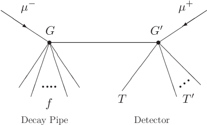
First we remind ourselves what is really measured in a neutrino factory. All we know is that the muons, say, with negative charge decay at an accumulate ring and wrong sign muons are observed in a detector located at a length $L$ away just after the time $L/c$, where $c$ is the light speed. This is depicted schematically in Fig.1.

Figure 1: What we really see in a neutrino factory.

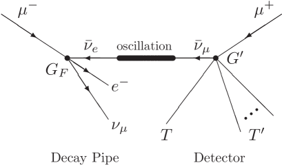
Since we know that there is the weak interaction process, we interpret such a wrong sign event as the evidence of the neutrino oscillation, $\bar{\nu}_{e}\rightarrow\bar{\nu}_{\mu}$, which is graphically represented in Fig.2.

Figure 2: Standard interpretation of a wrong sign event.

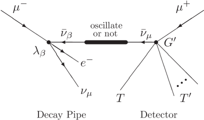
Now if there is a flavor-changing exotic interaction, e.g.,

$$\lambda(\bar{e}\gamma_{\mu}\mu)(\bar{\nu_{\mu}}\gamma^{\mu}\nu_{\alpha}),~{}~{}\alpha\neq e,$$ (3)

then we will have the same signal of a wrong sign muon, whose diagram is shown in Fig.3, just like that caused by the weak interaction and the neutrino oscillation.

Figure 3: Diagram which gives same signal as that given by Fig.2.

We cannot distinguish these two kinds of contribution. The quantum mechanics tells us that in this case, to get a transition rate, we first sum up these amplitudes and then square the summation. Therefore there is an interference phenomenon between several amplitudes in this process. Through this interference we get an enhancement of the effect of new physics, that is, we can make oscillation-enhanced search for new interactions with neutrinos.

More formally we illustrate this situation as follows. Denote the transition amplitude between the initial state $\mathcal{A}+\mathcal{T}$ and the final state $\mathcal{C}+\mathcal{U}$ through an intermediate state $\mathcal{B}$ as $\Phi({\mathcal{A},\mathcal{T}};{\mathcal{B}};{\mathcal{C},\mathcal{U}})$, where a final state $\mathcal{U}$ is one of the possible states which are unobserved like $\mathcal{B}$. The transition probability between $\mathcal{A}+\mathcal{T}$ and $\mathcal{C}+\mathcal{U}$, which is the absolute square of the sum of transition amplitudes with the same final state, is

$$P({\mathcal{A}+\mathcal{T}}\rightarrow{\mathcal{C}+\mathcal{U}})=\left|\sum_{\mathcal{B}}\Phi({\mathcal{A},\mathcal{T}};{\mathcal{B}};{\mathcal{C},\mathcal{U}})\right|^{2}.$$

The transition probability from $\mathcal{A}$ to $\mathcal{C}$ is given by summing up all unobserved initial states $\mathcal{T}$ and final states $\mathcal{U}$ as

$$P({\mathcal{A}}\rightarrow{\mathcal{C}})=\sum_{\mathcal{T},\mathcal{U}}P({\mathcal{A}+\mathcal{T}}\rightarrow{\mathcal{C}+\mathcal{U}}).$$ (4)

Furthermore suppose that the amplitude $\Phi({\mathcal{A},\mathcal{T}_{0}};{\mathcal{B}_{0}};{\mathcal{C},\mathcal{U}_{0}})$ is dominant over the amplitudes with intermediate states $\mathcal{B}(\neq\mathcal{B}_{0})$ and/or initial states $\mathcal{T}(\neq\mathcal{T}_{0})$ and/or final states $\mathcal{U}(\neq\mathcal{U}_{0})$. Then the dominant contribution to the probability $P({\mathcal{A}}\rightarrow{\mathcal{C}})$ is given by $P({\mathcal{A}}+{\mathcal{T}}_{0}\rightarrow{\mathcal{C}}+\mathcal{U}_{0})$ and deformed as

$$P({\mathcal{A}}\rightarrow{\mathcal{C}})\simeq P({\mathcal{A}+\mathcal{T}_{0}}\rightarrow\mathcal{C}+\mathcal{U}_{0})$$ (5)

$$~{}~{}~{}~{}~{}~{}~{}~{}~{}~{}~{}~{}~{}=\left|\Phi({\mathcal{A},\mathcal{T}_{0}};{\mathcal{B}_{0}};\mathcal{C},\mathcal{U}_{0})\right|^{2}$$ (6)

$$~{}~{}~{}~{}~{}~{}~{}~{}~{}~{}~{}~{}~{}~{}~{}~{}~{}+2{\rm Re}\left[\Phi({\mathcal{A},\mathcal{T}_{0}};{\mathcal{B}_{0}};\mathcal{C},\mathcal{U}_{0})^{*}\sum_{\mathcal{B}\neq\mathcal{B}_{0}}\Phi({\mathcal{A},\mathcal{T}_{0}};{\mathcal{B}};\mathcal{C},\mathcal{U}_{0})\right]$$ (7)

$$~{}~{}~{}~{}~{}~{}~{}~{}~{}~{}~{}~{}~{}~{}~{}~{}~{}+\left|\sum_{{\mathcal{B}}\neq{\mathcal{B}}_{0}}\Phi({\mathcal{A},\mathcal{T}_{0}};{\mathcal{B}};\mathcal{C},\mathcal{U}_{0})\right|^{2}.$$ (8)

Here the second term in eq.(7) is given by the interference among the leading amplitude $\Phi({\mathcal{A},\mathcal{T}_{0}};{\mathcal{B}_{0}};\mathcal{C},\mathcal{U}_{0})$ and the sub leading amplitudes $\Phi({\mathcal{A},\mathcal{T}_{0}};{\mathcal{B}}(\neq\mathcal{B}_{0});\mathcal{C},\mathcal{U}_{0})$. Note that the interference arises among the processes which have quite the same initial and final states, even if some of them are unobserved. “Same state” means a state with not only the same particle species but also all other same physical quantities, such as same energy and same helicity. This is very important in the calculation of the transition rate.

The leading amplitude is expected to arise from well known physics. On the other hand the amplitudes $\Phi({\mathcal{A},\mathcal{T}_{0}};{\mathcal{B}}(\neq\mathcal{B}_{0});\mathcal{C},\mathcal{U}_{0})$ is relatively small and may contain the contribution from new physics. However, even though $|\Phi({\mathcal{A},\mathcal{T}_{0}};{\mathcal{B}}(\neq\mathcal{B}_{0});\mathcal{C},\mathcal{U}_{0})|^{2}$ is very small, it would be possible for the interference term to be large. Thus even if the effect of new physics is not detectable due to systematic errors in a direct measurement, we may see the oscillation-enhanced effect of new physics.

In neutrino oscillation experiments, the state $\mathcal{A}$ consists of the state of the parent particle of neutrinos and $\mathcal{T}$ consists from the state of the target particle that interacts with a neutrino in a detector. The final state $\mathcal{C}$ corresponds to the state of the particle which can induce an identifiable event in a detector as a result of the interaction with the target particle ($\mathcal{T}$). Other final states $\mathcal{U}$ denote the states of all unobserved particles, which appear at both the neutrino-creation process and the detection process. The intermediate state $\mathcal{B}$ is interpreted as a neutrino state. The leading amplitude is given by the weak interaction and the neutrino oscillation, so the final state $\mathcal{U}_{0}$ is produced through the weak interaction, and the intermediate state $\mathcal{B}_{0}$ is a neutrino state which “oscillates” from a certain weak interaction eigenstate to same/another one. Even if there is no oscillation, different intermediate states $\mathcal{B}(\neq\mathcal{B}_{0})$ induced by exotic interactions give non-vanishing amplitudes for the total “oscillation” process. The new physics would violate the flavor conservation and/or the standard chiral property. Amplitudes which have all the same initial states $\mathcal{T}_{0}$ and final states $\mathcal{U}_{0}$ interfere with each other. It means that the leading amplitude from the weak interaction interferes with an exotic amplitude. In a neutrino-oscillation experiment such interference would give sub-leading contribution to the total probability. A large difference from the standard oscillation will be realized.

Figure 4: Transition rate for “$\bar{\nu}_{e}\rightarrow\bar{\nu}_{\mu}$”.

Figure 5: The transition probability of a wrong-sign muon production process through the neutrino “oscillation”. We denote $T$ and $T^{\prime}$ as the initial and the final state of the target particle of the neutrino in a detector. Large dots describe effective interactions. Effective interactions characterized by $G_{F}$ and $G_{T}$ are induced by the weak interaction. We assume that the other effective couplings, like $\lambda_{e}^{a}$, are caused by new physics and their superscripts identify the types of effective interactions. The bold line in each diagram stands for the neutrino oscillation including all matter effects induced by the weak interaction and exotic interactions. Here, appropriate integrations of momenta and summations of helicity states for unobserved particles are omitted.

Figure 6: The transition probability of a wrong-sign muon appearance process up to sub-leading contribution.

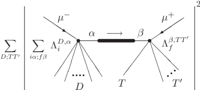
To put the situation concretely, we consider a wrong-sign muon production process through the neutrino oscillation $\bar{\nu}_{e}\rightarrow\bar{\nu}_{\mu}$. In this case the initial state $\mathcal{A}$ is $\mu^{-}$ and the observed final state $\mathcal{C}$ is $\mu^{+}$. The above consideration tells that we have to calculate the transition rate depicted in Fig.4. Namely eq.(4) corresponds to Fig.4: The correspondences for the other symbols are $\mathcal{T}\leftrightarrow T$ and $\mathcal{U}\leftrightarrow D+T^{\prime}$, respectively. In this process, the new physics effects contribute to three parts; the neutrino-creation process as mentioned above in eq.(3), the detection process, e.g.,

$$g(\bar{\nu_{e}}\gamma_{\mu}\mu)(\bar{d}\gamma^{\mu}u),$$ (9)

and the matter effect described as

$$H=2\sqrt{2}G_{F}n_{e}\left(\begin{array}[]{ccc}\epsilon^{m}_{ee}&\epsilon^{m}_{e\mu}&\epsilon^{m}_{e\tau}\\ \epsilon^{m*}_{e\mu}&\epsilon^{m}_{\mu\mu}&\epsilon^{m}_{\mu\tau}\\ \epsilon^{m*}_{e\tau}&\epsilon^{m*}_{\mu\tau}&\epsilon^{m}_{\tau\tau}\\ \end{array}\right),$$ (10)

where $n_{e}$ is the electron number density in matter. For anti-neutrinos such an exotic matter effect is given by $-H^{*}$. The interaction Hamiltonian of the exotic matter effect is induced in the similar way to the standard matter effect.

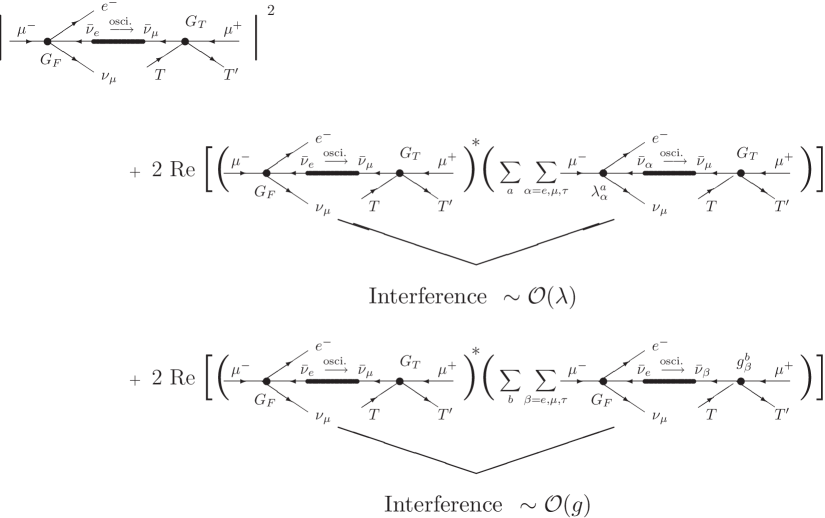
By expanding Fig.4, the transition probability of this process is illustrated in Fig.5. In Fig.5 the first diagram on the first line describes the contribution from the weak interaction and the oscillation process, where the unobserved state $\mathcal{U}_{0}$ corresponds to $\{e^{-}$, $\nu_{\mu}$ ,$T^{\prime}\}$. It gives the leading amplitude. The other diagrams on the first line in Fig.5 represent the effects of new physics, in which the states of neutrinos before and/or after the oscillation differ from the weak interaction case in flavor and/or chiral property. Since diagrams in the first line have completely the same final states $\mathcal{C}$ and $\mathcal{U}_{0}$, they interfere with each other. The diagrams on the second and the third line in Fig.5 have different final states form those of the first line, so that there is no interference with the weak interaction and it is expected that their contributions to the transition rate is negligibly small.

Thus eq.(5) is given by the diagram of the first line in Fig.5. Figure 6 shows the eq.(6) and eq.(7). The leading probability is proportional to $G_{F}^{2}G_{T}^{2}$ since it is known that exotic effective interactions are so small according to the direct searches, that $|\lambda|^{2}\ll|G_{F}|^{2}$ and $|g|^{2}\ll|G_{T}|^{2}$. However, the effect of new physics gives ${\mathcal{O}}(\lambda)$ and ${\mathcal{O}}(g)$ contribution to the signal of wrong sign muon due to the interference with the amplitude of the weak interaction. This fact makes the search for new physics possible in an oscillation-enhanced way. It gives relatively large effect. On the contrary, even if the stored muon are very high intense, a direct detection of an exotic decay process will be very difficult due to systematics since the probabilities of such processes are proportional to the squares of the effective coupling constants and hence is expected too small to be detected.

III Formalism and parameterization of an Interference effect with new physics in neutrino oscillation

In this section we consider the neutrino oscillation in the presence of new physics more concretely to get the analytic expression for the transition rate. Hereafter we consider only diagrams which interfere with that of the known physics, i.e., the weak interaction.

First we note that the amplitude for “neutrino oscillation” can be divided into three pieces: (1) Amplitude relevant with decay of a parent particle denoted as $A^{C}_{\alpha}$, here $C$ describes the type of interactions. For $\mu$ decay, as we will see in eq.(12) and (13), there are two types of interactions, $C=L,R$ while for $\pi$ decay we do not need this label. $\alpha$ distinguishes the particle species which easily propagates in the matter and make an interaction at a detector. (2) Amplitude representing a transition of these propagating particles, which are usually neutrinos, from one species $\alpha$ to another/same $\beta$ , denoted as $T_{\alpha\beta}$. (3) Amplitude responsible for producing a charged lepton $\l$ from a propagated particle $\beta$ at a detector, stood for by $D^{I}_{\beta l}$. Here $I$ denotes an interaction type. Using these notations we get the probability to observe a charged lepton $l^{\pm}$ at a detector as

$$P_{\mu^{-}\rightarrow l^{+}(l^{-})} = \left|\sum_{\alpha\beta CI}A^{C}_{\alpha}T_{\alpha\beta}D_{\beta l^{\pm}}^{I}\right|^{2}$$ (11)

$$= \sum_{\alpha\beta CI}\sum_{\alpha^{\prime}\beta^{\prime}C^{\prime}I^{\prime}}A^{C}_{\alpha}T_{\alpha\beta}D_{\beta l^{\pm}}^{I}A^{C^{\prime}*}_{\alpha^{\prime}}T_{\alpha^{\prime}\beta^{\prime}}^{*}D_{\beta^{\prime}l^{\pm}}^{I^{\prime}*}.$$

Therefore we can consider the effect of new physics separately for decay, propagation and detection processes.

First we consider the decay process of parent particles. Since all final states must be the same, for a neutrino factory, the exotic decays of muons which are $\mu^{-}\rightarrow e^{-}\nu_{\alpha}\bar{\nu}_{e}$ and $\mu^{-}\rightarrow e^{-}\nu_{\mu}\bar{\nu}_{\beta}$ can be amplified by the interference. Though in the presence of Majorana mass terms neutrinos and anti neutrinos can mix with each other, this effect is strongly suppressed by $m_{\nu}/E_{\nu}$. Therefore we do not have to consider decays into neutrino with opposite chirality such as $\mu^{-}\rightarrow e^{-}\bar{\nu}_{\mu}\bar{\nu}_{\beta}$ The former is relevant with $\mu^{-}\rightarrow l^{-}$ and the latter is relevant with $\mu^{-}\rightarrow l^{+}$. In other words, we can approximate neutrinos to be massless except for the propagation process. This fact and Lorentz invariance allow only two kinds of new interactions in this process. For a wrong-sign mode, the allowed two interactions are the $(V-A)(V-A)$ type,

$$2\sqrt{2}\lambda_{\alpha}(\bar{\nu_{\mu}}\gamma^{\rho}P_{L}\mu)(\bar{e}\gamma_{\rho}P_{L}\nu_{\alpha}),~{}~{}\alpha=\mu,\tau,$$ (12)

which has the same chiral property as the weak interaction but violates the flavor conservation, and the $(V-A)(V+A)$ type,

$$2\sqrt{2}\lambda^{\prime}_{\alpha}(\bar{\nu_{\mu}}\gamma^{\rho}\nu_{\alpha})(\bar{e}\gamma_{\rho}P_{R}\mu),~{}~{}\alpha=e,\mu,\tau.$$ (13)

The latter has different chiral property from the former, so that it gives different energy dependence to the transition rate. These exotic interactions interfere with the leading amplitude and contribute as next leading effects. Note that generally $\lambda$ and $\lambda^{\prime}$ are complex numbers.Grossman

In the case of the $(V-A)(V-A)$ type exotic interaction, we can introduce the interference effect by treating the initial state of oscillating neutrino as the superposition of all flavor eigenstates. On the $\mu^{-}\rightarrow\mu^{+}$ process, we can take initial neutrino $\bar{\nu}$ as

$$\bar{\nu}=\bar{\nu}_{e}+\epsilon_{\mu}\bar{\nu}_{\mu}+\epsilon_{\tau}\bar{\nu}_{\tau},$$ (14)

where $\epsilon_{\alpha}=\lambda_{\alpha}/G_{F}$. This simple treatment is allowed only for the $(V-A)(V-A)$ type interaction because of the same interaction form as the weak interaction except for difference of the coupling constant and the flavor of antineutrino. In this case we can generalize the initial neutrino for any flavor, using Y. Grossman’s source state notation Grossman , as,

$$\nu^{s}_{\beta}=U^{s}_{\beta\alpha}\nu_{\alpha},\quad\alpha,\beta=e,\mu,\tau,$$

$$U^{s}\equiv\begin{pmatrix}1&\epsilon^{s}_{e\mu}&\epsilon^{s}_{e\tau}\\ \epsilon^{s}_{\mu e}&1&\epsilon^{s}_{\mu\tau}\\ \epsilon^{s}_{\tau e}&\epsilon^{s}_{\tau\mu}&1\end{pmatrix}.$$ (15)

We can include the total exotic effect into the oscillation probability as

$$P_{\nu^{s}_{\alpha}\rightarrow\nu_{\beta}} =\left|\langle\nu_{\beta}|e^{-iHL}U^{s}_{\alpha\gamma}|\nu_{\gamma}\rangle\right|^{2}.$$ (16)

This treatment is also valid for the effect on the $\nu_{\mu}$ oscillation.

In the case of the $(V-A)(V+A)$ type exotic interaction, we cannot treat interference terms simply. The interference term between the weak interaction and an exotic interaction eq.(13) denoted as $P^{(1)}_{\mu\rightarrow l}$ gives the rate for the observation of the wrong sign charged lepton, which is interpreted normally as the oscillation from $\bar{\nu}_{e}\rightarrow\bar{\nu}_{l}$ in $\mu^{-}$ decay, as follows:

$$P^{(1)}_{{\mu}^{-}\rightarrow l^{+}} = \frac{1+\mathcal{P_{\mu}}}{2}\frac{1}{(2\pi)^{2}}\sum_{\rm{spin}}\int\frac{d^{3}p_{e}}{2E_{e}}\frac{d^{3}p_{\nu_{\mu}}}{2E_{\nu_{\mu}}}\delta^{4}(p_{\mu}-p_{\bar{\nu}}-p_{e}-p_{\nu_{\mu}})$$ (17)

$$~{}~{}~{}~{}~{}~{}~{}~{}~{}\times 2{\rm Re}\left[A_{e}^{L*}\sum_{\beta I}T_{e\beta}^{*}D^{I*}_{\beta l^{+}}\sum_{\alpha\beta^{\prime}I^{\prime}}A_{\alpha}^{R}T_{\alpha\beta^{\prime}}D_{\beta^{\prime}l^{+}}^{I^{\prime}}\right]$$

$$= \frac{1+\mathcal{P_{\mu}}}{2}\frac{8G_{F}}{\pi}m_{e}m_{\mu}E_{\nu}(|{\mathbf{p}}_{\mu}|-E_{\mu})\sum_{\alpha\beta\beta^{\prime}II^{\prime}}{\rm Re}[\lambda_{\alpha}^{\prime}T_{e\beta}^{*}D^{I*}_{\beta l^{+}}T_{\alpha\beta^{\prime}}D_{\beta^{\prime}l^{+}}^{I^{\prime}}],$$

where $\mathcal{P}_{\mu}$ is the polarization of the initial $\mu^{-}$, $E_{\nu}$ is $\nu$ energy, and ${\mathbf{p}}_{\mu}(E_{\mu})$ is $\mu$ momentum (energy).

In the case for the observation of the same sign charged lepton, which is interpreted as the oscillation from $\nu_{\mu}\rightarrow\nu_{l}$ in $\mu^{-}$ decay, as follows:

$$P^{(1)}_{{\mu}^{-}\rightarrow l^{-}} = \frac{1-\mathcal{P}_{\mu}}{2}\frac{8G_{F}}{\pi}m_{e}m_{\mu}E_{\nu}(|{\mathbf{p}}_{\mu}|-E_{\mu})\sum_{\alpha\beta\beta^{\prime}II^{\prime}}{\rm Re}[\lambda_{\alpha}^{\prime}T_{\mu\beta}^{*}D^{I*}_{\beta l^{-}}T_{\alpha\beta^{\prime}}D_{\beta^{\prime}l^{-}}^{I^{\prime}}],$$ (18)

For $\pi$ decay the situation is much simpler. In the presence of new physics there may be a flavor violating decay of $\pi$ such as $\pi^{-}\rightarrow\mu^{-}\nu_{\alpha}(\alpha=e,\tau)$. This effect changes the initial $\nu$ state;

$$\nu_{\mu}\longrightarrow\nu^{s}_{\mu}=\epsilon_{\mu e}^{s}\nu_{e}+\nu_{\mu}+\epsilon_{\mu\tau}^{s}\nu_{\tau}.$$ (19)

In this case we do not have to worry about the type of new physics which gives a flavor changing $\pi$ decay at a low energy scale. Due to kinematics, the energy and the helicity of the decaying particles, $\mu$ and $\nu$ are fixed.

Next we consider the propagation process. Exotic interactions also modify the Hamiltonian for neutrino propagation as NewPhysMatter ,

$$H_{\beta\alpha} =\frac{1}{2E_{\nu}}\left\{U_{\beta i}\begin{pmatrix}0&&\\ &\delta m_{21}^{2}&\\ &&\delta m_{31}^{2}\end{pmatrix}U^{\dagger}_{i\alpha}+\begin{pmatrix}\bar{a}+a_{ee}&a_{e\mu}&a_{e\tau}\\ {a_{e\mu}}^{*}&a_{\mu\mu}&a_{\mu\tau}\\ {a_{e\tau}}^{*}&{a_{\mu\tau}}^{*}&a_{\tau\tau}\end{pmatrix}_{\beta\alpha}\right\},$$ (20)

where $\bar{a}$ is the ordinary matter effect given by $2\sqrt{2}G_{F}n_{e}E_{\nu}$, $a_{\alpha\beta}$ is the extra matter effect due to new physics interactions, that is defined by $a_{\alpha\beta}=2\sqrt{2}\epsilon^{m}_{\alpha\beta}G_{F}n_{e}E_{\nu}$. Note that to consider the magnitude of the matter effect, the type of the interaction is irrelevant since in matter particles are at rest and hence the dependence on the chirality is averaged out.BGE

Finally we make a comment about new physics which affect a detection process. To consider this process we need the similar treatment to that at the decay process, that is, we have to separate contribution of new interactions following the difference of the chirality dependence. However to take into account new physics at a detector, the parton distribution and a knowledge about hadronization are necessary. Though we may wonder whether we can parameterize the effect of new physics at the detector $g/G_{T}$ as $\epsilon^{d}$ like $\epsilon^{s}$. It is expected that $\epsilon^{d}$ has a complicated energy dependence due to the parton distribution for example in a energy region of a neutrino factory. Consider the case that there is an elementary process from lepton flavor violating new physics including strange quark. To parameterize its effect we need both its magnitude and the distribution function of strange quark in nucleon which will show the dependence on the neutrino energy (more exactly, the transfered momentum from neutrino to strange quark). They are beyond our ability and hence we do not consider them further in this paper, though new physics which can affect the decay process have contribution to the detection process too.

IV numerical analysis

Let us discuss the feasibility to observe the signal induced by new physics. We will deal with both an upgraded conventional beam and a neutrino factory but present a little bit qualitatively different analysis in each experiment.

For a neutrino factory, we use following procedures: First, we assume the magnitude of the effects caused by new interactions. Next, we calculate the event numbers including the effects of new physics $N^{NP}$ and also calculate that based on the standard model $N^{SM}$. Then, we define the following quantity, so called $\chi^{2}$ function ,

$$\chi^{2} \equiv\sum_{i}^{\rm bin}\frac{\left|N^{NP}_{i}-N^{SM}_{i}\right|^{2}}{N^{SM}_{i}}$$

$$\equiv N_{\mu}M_{\rm det}X^{2}_{\rm\nu-fact},$$ (21)

where $i$ is the energy bin index, $N_{\mu}$ is the muon number, and $M_{\rm det}$ is the detector mass. To claim that new physics effects can be observed at 90% confidence level, it is required

$$\chi^{2}>\chi^{2}_{90\%},$$ (22)

and this condition is rewritten as

$$N_{\mu}M_{\rm det}>\frac{\chi^{2}_{90\%}}{X^{2}_{\rm\nu-fact}}.$$ (23)

From the above method, we can obtain the necessary muon number and the detector mass to observe the new physics effects at 90% confidence level.

On the other hand, there are some kinds of option on beam configurations for an upgraded conventional beam; wide band, narrow band, off axis, and so on. We discuss the event number of no-oscillated neutrino events at the detector $N_{\nu}$ unlike the case for a neutrino factory. The concrete procedure is almost the same as that for a neutrino factory. We separate $\chi^{2}$ function defined in first line of eq.(21) into two parts;

$$\chi^{2}\equiv N_{\nu}X^{2}_{\rm conv},$$ (24)

and get the necessary number of no-oscillated neutrino events from

$$N_{\nu}>\frac{\chi^{2}_{90\%}}{X^{2}_{\rm conv}}.$$ (25)

In the numerical calculation for a conventional beam, we consider the wide-band-beam like situation, whose flux distribution for energy is constant.

IV.1 $(V-A)(V-A)$ type new interaction

Here, we deal with the case that there are only $(V-A)(V-A)$ type new interactions in the lepton sector. In this case, we need to consider the effect represented in eqs.(15) and (20). Before making the presentation of the numerical calculations, we give the analytic expression for the sensitivities to understand the essential features. As we showed in section III, the interference terms between $(V-A)(V-A)$ type interactions and the weak interaction have the same dependence on the $\mu$ polarization leading term does. It can not be expected that the sensitivity to such interference term becomes better by the control of the parent $\mu$ polarization. We consider here an unpolarized muon beam. The “oscillation probability” is given by eq.(16) in this situation. More detailed calculations are presented in the Appendix.

IV.1.1 $\nu_{e}\rightarrow\nu_{\mu}$ channel in a neutrino factory

The analytic expression of probability for $\nu_{e}\rightarrow\nu_{\mu}$ given in the Appendix A shows that the effect due to $\epsilon^{m}_{\mu\tau}$ and $\epsilon^{s,m}_{\alpha\alpha}$ are irrelevant since these terms are proportional to $\sin^{2}2\theta_{13}\times\epsilon$ in the high energy region, so it is difficult to observe their effects. The flavor changing processes between muon and electron, e.g., $\mu\rightarrow e\gamma$, $\mu\leftrightarrow e$ conversion, are strictly constrained from experiments, and as we argue in the next section the box diagrams of the $\mu$-to-$e$ processes must relate to $\epsilon_{e\mu}^{s}$ and $\epsilon_{\mu e}^{s}$. Therefore, the magnitude of $\epsilon^{s}_{e\mu}$ has very severe bound and the terms depending on it are also not effective. Assuming some models, e.g., MSSM with right-handed neutrinos, it is expected that the magnitude of $\epsilon^{s}_{\alpha\beta}$ and $\epsilon^{m}_{\alpha\beta}$ are the same order because they are produced by similar diagrams. This is also discussed in the next section. We assume naively that the terms depending on $\epsilon^{m}_{e\mu}$ are constrained as $\epsilon^{s}_{e\mu}$. On the other hand, the $\tau$-to-$e$ processes do not give the tight bound to $\epsilon_{e\tau}^{s,m}$. Hence, we investigate the effect induced by $\epsilon^{s,m}_{e\tau}$ first.

Before surveying the required $N_{\mu}M_{\rm det}$ for each baseline $L$ and muon energy $E_{\mu}$, we see the behavior of contribution of $\epsilon_{e\tau}^{s,m}$ to the “oscillation probability” to consider the optimum setup for $L$ and $E_{\mu}$. In the high energy region such as the matter effect $\bar{a}$ is much greater than $\delta m_{31}^{2}$, the first order contribution of $\epsilon^{s,m}_{e\tau}$ to the transition probability, $\Delta P_{\nu_{e}\rightarrow\nu_{\mu}}\{\epsilon_{e\tau}\}$, is constructed by four parts that have the different $\epsilon_{e\tau}^{s,m}$ dependences:

$$\Delta P_{\nu_{e}\rightarrow\nu_{\mu}}\{\epsilon_{e\tau}\} =2s_{23}s_{2\times 23}s_{2\times 13}$$

$$\quad\times\Biggl{[}c_{13}^{2}\left(s_{\delta}{\rm Re}[\epsilon_{e\tau}^{s}]-c_{\delta}{\rm Im}[\epsilon_{e\tau}^{s}]\right)\left(\frac{\bar{a}}{4E_{\nu}}L\right)\left(\frac{\delta m_{31}^{2}}{4E_{\nu}}L\right)^{2}$$ (26a)

$$\qquad+c_{13}^{2}\left(c_{\delta}{\rm Re}[\epsilon^{s}_{e\tau}]+s_{\delta}{\rm Im}[\epsilon^{s}_{e\tau}]\right)\left\{1-\frac{1}{2}\left(\frac{\bar{a}}{4E_{\nu}}L\right)^{2}-s_{13}^{2}\left(\frac{\bar{a}}{4E_{\nu}}L\right)\left(\frac{\delta m_{31}^{2}}{4E_{\nu}}L\right)\right\}\left(\frac{\delta m_{31}^{2}}{4E_{\nu}}L\right)^{2}$$ (26b)

$$\qquad-c_{13}^{2}\left(s_{\delta}{\rm Re}[\epsilon_{e\tau}^{m}]+c_{\delta}{\rm Im}[\epsilon_{e\tau}^{m}]\right)\left(\frac{\bar{a}}{4E_{\nu}}L\right)\left(\frac{\delta m_{31}^{2}}{4E_{\nu}}L\right)^{2}$$ (26c)

$$\qquad-\frac{1}{3}s_{13}^{2}\left(c_{\delta}{\rm Re}[\epsilon_{e\tau}^{m}]-s_{\delta}{\rm Im}[\epsilon_{e\tau}^{m}]\right)\left\{\left(\frac{\bar{a}}{4E_{\nu}}L\right)+2\left(\frac{\delta m_{31}^{2}}{4E_{\nu}}L\right)\right\}\left(\frac{\bar{a}}{4E_{\nu}}L\right)\left(\frac{\delta m_{31}^{2}}{4E_{\nu}}L\right)^{2}\Biggr{]},$$ (26d)

where $s_{2\times ij}\equiv\sin 2\theta_{ij}$. Since we can suppose that $E_{\nu}$ is proportional to $E_{\mu}$ in a neutrino factory, $E_{\mu}$ and $L$ dependence of the sensitivity to each term can be approximated as

$$\chi^{2}\eqref{eq:HighEnergy_nuenumu_ETau_s_ReCosDelta}\propto\left\{1-\frac{1}{2}\left(\frac{\bar{a}}{4E_{\mu}}L\right)^{2}\right\}^{2}\times E_{\mu},\quad\chi^{2}({\rm\ref{eq:HighEnergy_nuenumu_ETau_s_ImCosDelta},\ref{eq:HighEnergy_nuenumu_ETau_m_ImCosDelta}})\propto\left(\frac{\bar{a}}{4E_{\mu}}L\right)^{2}\times E_{\mu},\quad\chi^{2}\eqref{eq:HighEnergy_nuenumu_ETau_m_ReCosDelta}\propto\left(\frac{\bar{a}}{4E_{\mu}}L\right)^{4}\times E_{\mu}.$$ (27)

All of eq.(27) are proportional to $E_{\mu}$, so the sensitivities must get better as the energy becomes higher.

Each of eq.(27) depends on $L$ in different way. $\chi^{2}\eqref{eq:HighEnergy_nuenumu_ETau_s_ReCosDelta}$ become tiny for longer baseline length within the region that we are now interested in. This fact means that a shorter baseline experiment has an advantage over a longer one to observe (26b)’s effect. By contrast with this, it is found that longer baseline will be better to search for the effects of (26a), (26c) and (26d).

Each of eq.(27) depends on the combinations of $\epsilon_{e\tau}^{s,m}$ and the CP phase $\delta$. What we observe is the combination of them. The effects of $\epsilon$’s can be sources of the CP-violation effect.Grossman In the discussion about the observation of the CP phase, this fact should be considered. The analytic expressions also show that the sensitivities are proportional to $|\epsilon|^{2}$.

Now, we show the results of the numerical calculations. The parameters that we use here are

$$\sin\theta_{12}=\frac{1}{2},\quad\sin\theta_{23}=\frac{1}{\sqrt{2}},\quad\sin\theta_{13}=0.1,$$

$$\delta m_{21}^{2}=5\times 10^{-5},\quad\delta m_{31}^{2}=3\times 10^{-3},$$ (28)

$$\delta=\frac{\pi}{2},$$

and take $|\epsilon|=3\times 10^{-3}$, which is a reference value for the feasibility to observe the effect by using the method of the oscillation enhancement. Except for $\epsilon_{e\mu}^{s,m}$ and $\epsilon_{\mu e}^{s}$, the constraints of the processes of charged lepton have not forbidden this magnitude of $\epsilon$’s.

Figure 7: Contour plots of the required $N_{\mu}M_{\rm det}$ to observe the new physics effects concerning $\epsilon_{e\tau}^{s,m}$ at 90% C.L. in $\nu_{e}\rightarrow\nu_{\mu}$ channel using a neutrino factory. From left to right: $(\epsilon_{e\tau}^{s},\epsilon_{e\tau}^{m})=(3.0\times 10^{-3},0)$, $(3.0\times 10^{-3}i,0)$, $(0,3.0\times 10^{-3})$, $(0,3.0\times 10^{-3}i)$. The uncertainties of theoretical parameters are not considered in these plots. As we point out in the text, when the uncertainties are taken into account, the sensitivities are completely lost. In Fig.7 to Fig.14, contours mean 0.01, 0.05, 0.1, 0.5, 1$\times 10^{21}\cdot 100{\rm kt}$.

Figure 8: Same as Fig.7, but here new interactions in both source and matter are taken into account. From left to right and top to bottom: $(\epsilon_{e\tau}^{s},\epsilon_{e\tau}^{m})=(3.0\times 10^{-3},3.0\times 10^{-3})$, $(3.0\times 10^{-3}i,3.0\times 10^{-3}i)$, $(3.0\times 10^{-3},3.0\times 10^{-3}i)$, $(3.0\times 10^{-3}i,3.0\times 10^{-3})$; $(3.0\times 10^{-3},-3.0\times 10^{-3})$, $(3.0\times 10^{-3}i,-3.0\times 10^{-3}i)$, $(3.0\times 10^{-3},-3.0\times 10^{-3}i)$, $(3.0\times 10^{-3}i,-3.0\times 10^{-3})$. These plots can be understood by addition or subtraction of the plots in Fig.7.

Fig.7 shows the required $N_{\mu}M_{\rm det}$ in the case where we do not take into account the uncertainties of the mixing parameters. We can check whether the approximated equations, eq.(27), are correct from the behavior of the plots. As eq.(26) implies, contribution from the new interaction depends on the combinations of $\epsilon$ and $\delta$. We take $\delta=\pi/2$, so we can extract each term of eq.(26) by taking $\epsilon_{e\tau}^{s,m}$ pure real and imaginary. Therefore, the plots of Fig.7 from left to right correspond to the required data size to observe each term in eq.(26a) to eq.(26d) respectively. The behavior of these plots is consistent with the expectations from the analytic expressions in eq.(27). To consider realistic situations, the new physics effects in both source and matter must be taken into account simultaneously. We present Fig.8 as the plots in the cases where the same magnitude of new effects in both source and matter are introduced. They show that the total effects are given by the simple summation of each effect.

In realistic situations the uncertainties of the theoretical parameters have to be taken into account. Once the uncertainties are introduced, it can be expected that the sensitivities shown in Figs.7 and 8 will be spoiled completely. The $\epsilon_{e\tau}^{s,m}$ effect can be absorbed easily into the main (unperturbed) part of oscillation by adjusting the theoretical parameters since the effects have the same energy dependence as the main part has. Indeed, taking into account these uncertainties, the sensitivities to $\epsilon_{e\tau}^{s,m}$ are completely washed out. Therefore, we have to look for the terms whose energy dependence differ from that of the main oscillation term in the high energy region. In $\nu_{e}\rightarrow\nu_{\mu}$ channel, the effects caused by $\epsilon_{e\mu}^{s,m}$ have such energy dependence. It can be represented analytically in the high energy region as

$$\Delta P_{\nu_{e}^{s}\rightarrow\nu_{\mu}}\{\epsilon_{e\mu}\} =2s_{23}s_{2\times 13}$$

$$\quad\times\Biggl{[}\left(s_{\delta}{\rm Re}[\epsilon^{s}_{e\mu}]-c_{\delta}{\rm Im}[\epsilon^{s}_{e\mu}]\right)$$

$$\qquad\quad\times\Biggl{\{}1-\frac{2}{3}\left(\frac{\bar{a}}{4E_{\nu}}L\right)^{2}+\frac{2}{3}\left(2c_{2\times 13}-3c_{23}^{2}c_{13}^{2}\right)\left(\frac{\bar{a}}{4E_{\nu}}L\right)\left(\frac{\delta m_{31}^{2}}{4E_{\nu}}L\right)\Biggr{\}}\left(\frac{\delta m_{31}^{2}}{4E_{\nu}}L\right)$$ (29a)

$$\qquad-\left(c_{\delta}{\rm Re}[\epsilon^{s}_{e\mu}]+s_{\delta}{\rm Im}[\epsilon^{s}_{e\mu}]\right)$$

$$\qquad\quad\times\Biggl{[}\left\{1-\frac{1}{3}\left(\frac{\bar{a}}{4E_{\nu}}L\right)^{2}\right\}\left(\frac{\bar{a}}{4E_{\nu}}L\right)$$

$$\qquad\qquad\qquad-\left\{1-2s_{23}^{2}c_{13}^{2}-\left(1-c_{13}^{2}\left(2-\frac{4}{3}c_{23}^{2}\right)\right)\left(\frac{\bar{a}}{4E_{\nu}}L\right)^{2}\right\}\left(\frac{\delta m_{31}^{2}}{4E_{\nu}}L\right)\Biggr{]}\left(\frac{\delta m_{31}^{2}}{4E_{\nu}}L\right)$$ (29b)

$$\qquad+2c_{23}^{2}\left(s_{\delta}{\rm Re}[\epsilon_{e\mu}^{m}]+c_{\delta}{\rm Im}[\epsilon_{e\mu}^{m}]\right)\left(\frac{\bar{a}}{4E_{\nu}}L\right)\left(\frac{\delta m_{31}^{2}}{4E_{\nu}}L\right)^{2}$$ (29c)

$$\qquad+2\left(c_{\delta}{\rm Re}[\epsilon_{e\mu}^{m}]-s_{\delta}{\rm Im}[\epsilon_{e\mu}^{m}]\right)$$

$$\qquad\quad\times\Biggl{\{}1-\frac{1}{3}\left(\frac{\bar{a}}{4E_{\nu}}L\right)^{2}+\left(c_{23}^{2}s_{13}^{2}+\frac{2}{3}s_{23}^{2}c_{2\times 13}\right)\left(\frac{\bar{a}}{4E_{\nu}}L\right)\left(\frac{\delta m_{31}^{2}}{4E_{\nu}}L\right)\Biggr{\}}\left(\frac{\bar{a}}{4E_{\nu}}L\right)\left(\frac{\delta m_{31}^{2}}{4E_{\nu}}L\right)\Biggr{]}.\qquad$$ (29d)

Contribution for the transition probability labeled (29a), (29b) and (29d) depends on $1/E_{\mu}$. Consequently, the sensitivities to the terms must be robust against the uncertainties of the theoretical parameters since in the high energy region they can be distinguished from the main oscillation part by observing the energy dependence. The claims mentioned above are confirmed numerically by Fig.9 and 10. By comparison of these graphs, we can see that the sensitivities to observe the contribution of (29a), (29b) and (29d) do not suffer from the uncertainties. Incidentally, we note that though the uncertainties wreck the sensitivity to (29c) since it is proportional to $1/E_{\mu}^{2}$, the $\epsilon_{e\mu}^{m}$ second order term brings constant contribution for energy and this signal does not vanish.

Figure 9: Contour plots of the required $N_{\mu}M_{\rm det}$ to observe the new physics effects concerning $\epsilon_{e\mu}^{s,m}$ at 90% C.L. in $\nu_{e}\rightarrow\nu_{\mu}$ channel when there is no uncertainty for theoretical parameters. From left to right: $(\epsilon_{e\mu}^{s},\epsilon_{e\mu}^{m})=(3.0\times 10^{-3},0)$, $(3.0\times 10^{-3}i,0)$, $(0,3.0\times 10^{-3})$, $(0,3.0\times 10^{-3}i)$. Each plot corresponds to the sensitivities to eq.(29a)$\sim$eq.(29d) respectively.

Figure 10: Same as Fig.9, but here each parameter has 10% uncertainty.

IV.1.2 $\nu_{\mu}\rightarrow\nu_{\mu}$ channel in a neutrino factory

Only the effect that depend on $\epsilon_{\mu\tau}^{s,m}$ will be large enough to be observed in $\nu_{\mu}\rightarrow\nu_{\mu}$ disappearance channel. As we show in the next section, this quantity is not strongly bound by the charged lepton processes. The analytic expressions for the terms concerning $\epsilon_{\mu\tau}^{s,m}$ (see the Appendix B) indicate two facts: (1) this channel sensitive only to the real part of $\epsilon_{\mu\tau}^{m}$, and (2) the effect that comes from the real part of $\epsilon_{\mu\tau}^{s}$ will be small in the assumed parameter region. In addition, it shows that the terms depending on $\epsilon_{\mu\tau}^{s,m}$ are hard to be absorbed by the uncertainty of the theoretical parameters. Note that these terms do not depend on the CP phase $\delta$, that is, it is expected that we can get information on the phases of $\epsilon_{\mu\tau}^{s,m}$. The sensitivity plots calculated numerically are shown in Fig.11. They behave as expected by the analytic expressions. The uncertainties of the theoretical parameters do not affect the observability since the terms that depend on $1/E_{\mu}$ do not vanish in the high energy region. The sensitivities depend strongly on the phase of $\epsilon_{\mu\tau}^{s,m}$ but do not depend on $\delta$. We can directly know the phase of the lepton-flavor violation process without care of $\delta$.

Figure 11: Contour plots of the required $N_{\mu}M_{\rm det}$ to observe the new physics effects concerning $\epsilon_{\mu\tau}^{s,m}$ at 90% C.L. in $\nu_{\mu}\rightarrow\nu_{\mu}$ channel. All theoretical parameters are assumed to have 10% uncertainty. From left to right, each plot corresponds to $(\epsilon_{\mu\tau}^{s},\epsilon_{\mu\tau}^{m})=(3.0\times 10^{-3},0)$, $(3.0\times 10^{-3}i,0)$, $(0,3.0\times 10^{-3})$, $(0,3.0\times 10^{-3}i)$.

IV.1.3 Channels with $\tau$ and $e$ observation in a neutrino factory

The technologies for tau observation in $\nu_{\tau}$ detection OPERA and the charge identification of electron to distinguish $\nu_{e}$ with $\bar{\nu}_{e}$ Rubbia are under R & D. If it is possible to observe these particles clearly, what can we get ?

In $\nu_{e}\rightarrow\nu_{\tau}$ channel, we can explore $\epsilon_{e\tau}^{s,m}$ (see Fig.12). The uncertainties of the theoretical parameters will not disturb the observability. In $\nu_{\mu}\rightarrow\nu_{\tau}$ channel, all we can observe is only the effect of $\epsilon_{\mu\tau}^{s,m}$ (see Fig.13). In comparison with $\nu_{\mu}\rightarrow\nu_{\mu}$ channel, we will not have so much benefit in terms of sensitivities to the magnitude of $\epsilon$. However in this channel unlike $\nu_{\mu}\rightarrow\nu_{\mu}$ channel, the observable must depend on the combination of the $\epsilon_{\mu\tau}^{s,m}$’s phase and the CP phase $\delta$, that is, the observation in these two channels are qualitatively different. In $\nu_{\mu}\rightarrow\nu_{e}$ channel, we can search the effect of not $\epsilon^{s}_{e\mu}$ but $\epsilon^{s}_{\mu e}$ at the muon decay process and the effect of $\epsilon^{m}_{e\mu}$ at the propagation process just like $\nu_{e}\rightarrow\nu_{\mu}$ channel (see Fig.14). In $\nu_{e}\rightarrow\nu_{e}$ disappearance channel, oscillation effects themselves are much smaller than the no-oscillation signal. Though some effects of new physics give the different energy dependence from the main oscillation term, we will not be able to get any information for oscillation-enhanced new physics.

Figure 12: Contour plots of the required $N_{\mu}M_{\rm det}$ to observe the new physics effects concerning $\epsilon_{e\tau}^{s,m}$ at 90% C.L. in $\nu_{e}\rightarrow\nu_{\tau}$ channel. All theoretical parameters are assumed to have 10% uncertainty. From left to right, each plot corresponds to $(\epsilon_{e\tau}^{s},\epsilon_{e\tau}^{m})=(3.0\times 10^{-3},0)$, $(3.0\times 10^{-3}i,0)$, $(0,3.0\times 10^{-3})$, $(0,3.0\times 10^{-3}i)$.

Figure 13: Same as Fig.11, but $\nu_{\mu}\rightarrow\nu_{\tau}$ channel.

Figure 14: Contour plots of the required $N_{\mu}M_{\rm det}$ to observe the new physics effects concerning $\epsilon_{\mu e}^{s}$ and $\epsilon^{m}_{e\mu}$ at 90% C.L. in $\nu_{\mu}\rightarrow\nu_{e}$ channel. All theoretical parameters are assumed to have 10% uncertainty. From left to right, each plot corresponds to $(\epsilon_{\mu e}^{s},\epsilon_{e\mu}^{m})=(3.0\times 10^{-3},0)$, $(3.0\times 10^{-3}i,0)$, $(0,3.0\times 10^{-3})$, $(0,3.0\times 10^{-3}i)$.

IV.2 $(V-A)(V+A)$ type interactions

The signals of $(V-A)(V+A)$ type interactions are hard to be observed because they are suppressed by the factor, $m_{e}/m_{\mu}$. The interference term between the leading term and $(V-A)(V+A)$ type ones has different polarization dependence from that of the leading contribution unlike $(V-A)(V-A)$ type new interaction. If we can make good use of this fact, then we may be able to expect to gain somewhat better sensitivity. As we saw in eqs.(17) and (18), the utilization of the muon polarization works only in $\nu_{\mu}\rightarrow\nu_{\alpha}$. Figure.15 describes the sensitivity to ${\epsilon^{\prime}}_{\mu\tau}^{s}(\equiv\lambda^{\prime}/G_{F})$ in $\nu_{\mu}\rightarrow\nu_{\tau}$ channel. We can gain a little, but have no advantage over a direct search against our expectation.

Figure 15: Contour plots of the required $N_{\mu}M_{\rm det}$ to observe the $(V-A)(V+A)$ type new interaction, ${\epsilon^{\prime}}_{\mu\tau}^{s}=3.0\times 10^{-3}i$, at 90% C.L. in $\nu_{\mu}\rightarrow\nu_{\tau}$ channel. Contours mean 1, 5, 10, 50, 100$\times 10^{21}\cdot 100{\rm kt}$. Here, the uncertainties of the theoretical parameters are not considered. From left to right, each plot corresponds to $\mathcal{P_{\mu}}=$0.99, 0, $-0.99$.

IV.3 $\nu_{\mu}\rightarrow\nu_{e,\mu,\tau}$ channel in an upgraded conventional beam

In an experiment using a conventional beam, there are some different points from the case of a neutrino factory. Since we consider two body decay of $\pi$’s, the created charged lepton and the neutrino have the fixed helicity whatever new physics is. It means that we do not have to worry the type of a new interaction. We can always parameterize the effect of new physics concerning $\pi$ decay by $\epsilon^{s}_{\mu e}$ and $\epsilon^{s}_{\mu\tau}$. When we consider a new source interaction, new interactions between neutrino and nucleon must be introduced not only in matter but also in detector. However to consider such effects we have to treat complicated hadronic processes, so we do not consider the relation between these two effects. The contribution to the source and the matter effect is not always generated by the same new interactions. Hence, we can suppose that different magnitude interaction in each process.

As it became clear in analysis for a neutrino factory, all we can probe is the contribution of $\epsilon_{\mu e}^{s}$, $\epsilon_{e\mu}^{m}$ in $\nu_{\mu}\rightarrow\nu_{e}$ channel and that of $\epsilon_{\mu\tau}^{s,m}$ in $\nu_{\mu}\rightarrow\nu_{\mu,\tau}$ channel. However, new interactions in matter can not be observed in the energy and the baseline regions that we assume here and hence we do not study their effect. The numerical results for the necessary number of no-oscillated neutrinos $N_{\nu}$ are shown in Fig.16, Fig.17, and Fig.18. The neutrino event number of current proposed experiments is estimated of $\mathcal{O}(10^{3}\sim 10^{4})$, and $\mathcal{O}(10^{2})$ times larger exposure is expected in the next generation.

Figures 16, 17 and 18 show that the sensitivity strongly depends on the complex phase of $\epsilon$’s. This fact means that the observations give us information of the phase in lepton-flavor-violation interactions. Depending on models, some interesting issues are revealed. In the next section, we discuss models which may give the significant $\epsilon$’s. As we point out above, $\epsilon$’s for a neutrino factory and a conventional beam have different dependence on new interactions. Hence, it is important for new physics search to compare the results of a neutrino factory and that of a conventional beam.

Figure 16: Contour plots of the required no-oscillated neutrino number, $N_{\nu}$, to observe the new physics effects concerning $\epsilon_{\mu e}^{s}$ at 90% C.L. in $\nu_{\mu}\rightarrow\nu_{e}$ channel using an upgraded conventional beam. All theoretical parameters are assumed to have 10% uncertainty. From left to right, each plot corresponds to $\epsilon_{\mu e}^{s}=3.0\times 10^{-3}$, $3.0\times 10^{-3}i$. In this energy and baseline region, a experiment does not sensitive to new interactions in matter. In Fig.16, Fig.17, and Fig.18, contours mean 2, 4, 6, 8, 10 $\times 10^{5}$ no-oscillated neutrinos.

Figure 17: Contour plots of the required no-oscillated neutrino number, $N_{\nu}$, to observe the new physics effects concerning $\epsilon_{\mu\tau}^{s}$ at 90% C.L. in $\nu_{\mu}\rightarrow\nu_{\mu}$ channel using an upgraded conventional beam. All theoretical parameters are assumed to have 10% uncertainty. From left to right, each plot corresponds to $\epsilon_{\mu\tau}^{s}=3.0\times 10^{-3}$, $3.0\times 10^{-3}i$.

Figure 18: Same as Fig.17, but $\nu_{\mu}\rightarrow\nu_{\tau}$ channel.

IV.4 short summary for numerical analysis

For a neutrino factory:

• In $\nu_{\alpha}\rightarrow\nu_{\beta}$, $(\alpha=e,\mu,$ $\beta=e,\mu,\tau)$ appearance channel, the observable effects of new $(V-A)(V-A)$ interactions come only from $\epsilon_{\alpha\beta}^{s,m}$. The others are too small or too vulnerable against the adjustment of the theoretical parameters. Note that $\delta$ and $\epsilon$’s phase are correlated. Namely the measured values are a certain combination of $\delta$ and $\epsilon$.

• In $\nu_{\mu}\rightarrow\nu_{\mu}$ disappearance channel, we can measure $\epsilon_{\mu\tau}^{s,m}$ depending on their phase. In other words, the signal includes information of the phase. Furthermore, there is no correlation between $\delta$ and $\epsilon$, so the measurement tells us directly the phase concerning the lepton-flavor violating process. In $\nu_{e}\rightarrow\nu_{e}$ disappearance channel, we can not get anything for new interactions in the oscillation enhanced way.

• The $\chi^{2}$ is proportional to $|\epsilon|^{2}$. The expected sensitivity is to $|\epsilon|\gtrsim\mathcal{O}(10^{-4})$ by using this methodology.

• When the situations that new interactions exist not only in the source but also in the matter effect are considered, we can easily understand the sensitivity by simply adding each effect.

• Oscillation-enhanced effects for the $(V-A)(V+A)$ type interactions are strongly suppressed by $m_{e}/m_{\mu}$, so we can not get an advantage over a direct measurement.

For an upgraded conventional beam:

• We do not have to care the types of new interactions in the source. The analyses for the feasibility are similar to that of $(V-A)(V-A)$ type for a neutrino factory. In the assumed energy and baseline region, there is no sensitivity to the new effect in matter.

• The $\epsilon$’s for a conventional beam have different dependence from those for a neutrino factory on new interactions. Therefore, the comparison between two methods makes clear the species of new physics.

	$\epsilon_{e\mu}^{s,m}$, $(\epsilon_{\mu e}^{s})$	$\epsilon_{e\tau}^{s,m}$	$\epsilon_{\mu\tau}^{s,m}$
bound from charged lepton processes	$5\times 10^{-5}$	—	—
$\nu_{e}\rightarrow\nu_{\mu}$	$\triangle$	$\triangle$	$\times$
$\nu_{\mu}\rightarrow\nu_{\mu}$	$\times$	$\times$	$\circ$
$\nu_{e}\rightarrow\nu_{\tau}$	$\times$	$\circ$	$\triangle$
$\nu_{\mu}\rightarrow\nu_{\tau}$	$\times$	$\triangle$	$\circ$
$\nu_{\mu}\rightarrow\nu_{e}$	$\triangle$	$\times$	$\times$
$\nu_{e}\rightarrow\nu_{e}$	$\times$	$\times$	$\times$

Table 1: Summary on the feasibility of $(V-A)(V-A)$ type new interactions.

V Indications to exotic decays from various models

In this section we discuss models which give exotic interactions interfering with the weak interaction in the neutrino oscillation and survey to which process those exotic interactions contribute. We should consider models which give an explanation for the smallness of the neutrino masses and the lepton mixings. In those models we can expect that flavor violating processes are induced, and since to explain the neutrino masses and the lepton mixings we need to introduce sources of flavor violations.

There are well-known two types of models which explain the smallness of the neutrino masses and the lepton mixings. One is a seesaw type seasaw and the other is a radiative type zee . These models induce other flavor violating effects generally. Such other flavor violating contribution could be large enough to give observable effects for neutrino oscillation experiments through the interfering effects. We now consider these two types of models concerning mainly on supersymmetric models and study how large the exotic effective interactions are.

V.1 Supersymmetric models with right-handed neutrinos

Among the promising extensions of the standard model, a supersymmetric standard (or grand unified) model with right-handed neutrinos is often considered. In this class of models, if the gravity-induced supersymmetry breaking is employed, through the renormalization effect, the large flavor violating slepton masses are induced Bor , even if at the cutoff scale there is no flavor violating slepton mass.

Figure 19: (1) An Example of one-loop diagrams contributing to the $\mu$ decay and the matter effect. (2) An Example of tree diagrams contributing to the $\pi$ decay, the matter effect and the detection process. Where $\delta m^{2}_{\tilde{l}}$ denotes an off-diagonal element of the mass matrix for sleptons which violates the lepton flavor.

Due to the lepton flavor violating masses, one-loop box diagrams constructed by propagations of superpartners induce exotic effective $(V-A)(V-A)$ interactions, which contribute to the decay side, the matter effect and the detection side all together. One of effective interactions contributing to the decay side in oscillation experiments based on a muon beam is drawn in Fig19-(1). This gives $\epsilon_{\mu\tau}^{s}$. There is a constraint on the magnitude of Fig19-(1) from the lepton flavor violating decays of $\tau$ such as $\tau\rightarrow\mu\gamma$ and $\tau\rightarrow\mu ee$. However, these constraints are not so strict and $\epsilon_{\mu\tau}^{s}$ can be of ${\mathcal{O}}(10^{-3})$. This type of the effective interaction also induces the matter effect similarly replacing $\nu_{e}$ with $e$ and $\mu$ with $\nu_{\mu}$ respectively, and also $\epsilon^{m}_{\mu\tau}$ can be of ${\mathcal{O}}(10^{-3})$. By changing the external legs in Fig 19-(1), we can draw similar diagrams for four-lepton couplings which violate the lepton flavor, and using them we can estimate how large values the $\epsilon^{s,m}$’s are in each model and experimentally. They can contribute to the $\mu$ decay and the matter effects.

In addition, there are effective interactions generated by one-loop diagrams including squark propagators as Fig19-(2). These kinds of diagrams can contribute to the detection processes and the matter effects. Furthermore they can contribute to the $\pi$ decay.

These two kinds of diagrams affect the oscillation in a neutrino factory and a conventional beam differently. By comparing the results of these two experiments, we may have some information on the scalar masses. For example, if the squark masses are much heavier than the slepton masses, then only the figures of the type Fig19-(1) contribute to the oscillation phenomena, and hence there is a difference between “oscillation probabilities” in these two experiments. On the other hand if the magnitudes of the scalar masses are comparable, these two experiments are affected from new physics in the decay side, the matter effect and the detection side similarly.

It is important that we can get information on the phases of $\epsilon$’s. Their phases arise from the phases of the flavor changing slepton masses, whose origins are the Yukawa couplings for $\nu_{L}$ and $\nu_{R}$ at the high energy scale. We may be able to acquire information on the phases of Dirac-Yukawa couplings.

V.2 Models with radiatively induced neutrino masses

Figure 20: (1) Examples of tree diagrams contributing to the $\mu$ decay and the matter effect. (2) An Example of tree diagrams contributing to the $\pi$ decay, the matter effect and the detection process. The first diagram (1) induces both $(V-A)(V-A)$ type and $(V-A)(V+A)$ type interactions for the muon decay and the matter effect. The second diagram (2) induces $(V-A)(V+A)$ type interactions only, which contribute to the matter effect.

There are many kinds of models in which the neutrino masses and the lepton mixings are radiatively induced. Among them we consider supersymmetric models with R-parity violating terms. A most general superpotential which breaks R-parity is

$$W_{\rm RPV}=\lambda_{\alpha\beta\gamma}L_{\alpha}L_{\beta}E^{c}_{\gamma}+\lambda^{\prime}_{\alpha\beta\gamma}L_{\alpha}Q_{\beta}D^{c}_{\gamma}+\lambda^{\prime\prime}_{\alpha\beta\gamma}U^{c}_{\alpha}D^{c}_{\beta}D^{c}_{\gamma}+\mu^{\prime}_{\alpha}L_{\alpha}H_{U\alpha},$$ (30)

where $\lambda_{\alpha\beta\gamma}=-\lambda_{\beta\alpha\gamma},\lambda^{\prime\prime}_{\alpha\beta\gamma}=-\lambda^{\prime\prime}_{\alpha\gamma\beta}$. $L_{\alpha}$, $E^{c}_{\alpha}$, $Q_{\alpha}$, $U_{\alpha}$, $D^{c}_{\alpha}$ and $H_{U\alpha}$ are the superfields corresponding to the lepton doublets, the right-handed charged leptons, the quark doublets, the right-handed up-type-quarks, the down-type quarks and the up-type Higgs doublet respectively. Three trilinear terms are allowed if the R-parity is broken generally. However there is no reason why all R-parity violating terms should be included at the same time. For example, we forbid interactions proportional to $\lambda^{\prime\prime}_{\alpha\beta\gamma}$ by imposing the baryon-number conservation to avoid rapid proton decay. To induce small masses for neutrinos, the first term or the second term in eq.(30) must be included. For example the first term in eq.(30) has interactions described as

$${\mathcal{L}}=\lambda_{\alpha\beta\gamma}(\bar{\nu}^{c}_{\alpha L}e_{\beta L}\tilde{e}_{\gamma R}^{*}+\bar{e}_{\gamma R}\nu_{\alpha L}\tilde{e}_{\beta L}+\bar{e}_{\gamma R}e_{\beta L}\tilde{\nu}_{\alpha L}-(\alpha\leftrightarrow\beta))+{\rm H.c}.$$ (31)

These interactions work in a same way as those of the Zee model.zee Namely, sleptons interact with charged leptons and neutrinos as the Zee boson, and the small neutrino masses and the lepton mixings are induced radiatively. Such interactions induce $(V-A)(V-A)$ type and $(V-A)(V+A)$ type effective four-lepton interactions which violate the lepton flavor (see Fig.20). These affect oscillation experiments through the interference with the weak interaction. Since there are only four-lepton type effective interactions, we would be able to see the difference between “oscillation probabilities” in two different experiments. In the case of a neutrino factory, they affect both the decay side and the matter effect all together, while in the case of a conventional beam they affect only the matter effect. From these kinds of Fig.20-(1) $\epsilon^{s,m}_{\mu\tau}$ and $\epsilon^{s}_{e\tau}$ are induced. In this case the magnitudes of $\epsilon$’s could be larger than the case in the previous subsection.

Interactions generated by the second term in eq.(30), are described as

$${\mathcal{L}}=\lambda_{\alpha\beta\gamma}^{\prime}V^{KM}_{\beta\delta}(\bar{\nu}^{c}_{\alpha L}d_{\delta L}\tilde{d}_{\gamma R}^{*}+\bar{d}_{\gamma R}\nu_{\alpha L}\tilde{d}_{\delta L}+\bar{d}_{\gamma R}d_{\delta L}\tilde{\nu}_{\alpha L})$$

$$~{}~{}~{}~{}~{}~{}+\lambda_{\alpha\beta\gamma}^{\prime}(\bar{u}^{c}_{\beta L}e_{\alpha L}\tilde{d}_{\gamma R}^{*}+\bar{d}_{\gamma R}e_{\alpha L}\tilde{u}_{\beta L}+\bar{d}_{\gamma R}u_{\beta L}\tilde{e}_{\alpha L})+{\rm H.c.},$$ (32)

where $V^{KM}$ is the mixing matrix for the quark sector. In this case squarks work as the Zee boson similarly. These interactions induce effective four-Fermi interactions with the lepton flavor violation, as drawn in Fig.20-(2). They affect the matter effect and the detection process in both experiments based on a muon beam and on a conventional beam. For a conventional beam, there is an additional interference in the decay side. Therefore if the R-parity violating term is limited only to the second term in eq.(30), then we also expect to be able to make sure the existence of such terms by comparison with the two different experiments.

V.3 General properties of the effective four-lepton interactions and order estimation for their couplings.

Without assuming physics that gives the effective four-lepton interactions containing two left-handed neutrinos and two charged leptons with the lepton flavor violation, we can classify two types of such interactions from Lorentz invariance as the $(V-A)(V-A)$ type and the $(V-A)(V+A)$ type generally.

The flavor violating four-lepton couplings with the $(V-A)(V-A)$ type are classified into two categories: SU(2)_L singlet type,

$$h_{\alpha\beta\gamma\delta}(\bar{l}_{\alpha}C\bar{l}_{\beta})(l_{\gamma}C^{\dagger}l_{\delta})$$ (33)

$$=-\frac{1}{2}h_{\alpha\beta\gamma\delta}(\bar{l}_{\alpha}\gamma^{\mu}l_{\delta})(\bar{l}_{\beta}\gamma_{\mu}l_{\gamma})$$

$$=\frac{1}{2}h_{\alpha\beta\gamma\delta}h_{\alpha\beta\gamma\delta}(\bar{e}_{\alpha L}C\bar{\nu}_{\beta L}-\bar{\nu}_{\alpha L}C\bar{e}_{\beta L})({e}_{\gamma L}C^{\dagger}{\nu}_{\delta L}-\nu_{\gamma L}C^{\dagger}{e}_{\delta L}),$$

and triplet type,

$$g_{\alpha\beta\gamma\delta}(\bar{l}_{\alpha}\tau^{a}C\bar{l}_{\beta})(l_{\gamma}C^{\dagger}\tau^{a}l_{\delta})$$ (34)

$$=-\frac{1}{2}g_{\alpha\beta\gamma\delta}(\bar{l}_{\alpha}\tau^{a}\gamma^{\mu}l_{\delta})(\bar{l}_{\beta}\tau^{a}\gamma_{\mu}l_{\gamma})$$

$$=g_{\alpha\beta\gamma\delta}\left\{(\bar{e}_{\alpha L}C\bar{\nu}_{\beta L}+\bar{\nu}_{\alpha L}C\bar{e}_{\beta L})(e_{\gamma L}C^{\dagger}\nu_{\delta L}+\nu_{\gamma L}C^{\dagger}e_{\delta L})\right.$$

$$~{}~{}~{}~{}\left.+2(\bar{\nu}_{\alpha L}C\bar{\nu}_{\beta L})(\nu_{\gamma L}C^{\dagger}\nu_{\delta L})+2(\bar{e}_{\alpha L}C\bar{e}_{\beta L})(e_{\gamma L}C^{\dagger}e_{\delta L})\right\}.$$

Here $\l_{\alpha}$ is a lepton doublet with flavor $\alpha$ and $\tau^{a}$ is a Pauli matrix. Due to the SU(2)_L invariance coupling constants must satisfy $h_{\alpha\beta\gamma\delta}=-h_{\beta\alpha\gamma\delta}=-h_{\alpha\beta\delta\gamma}$ and $g_{\alpha\beta\gamma\delta}=g_{\beta\alpha\gamma\delta}=g_{\rho\sigma\delta\gamma}$. Above two interactions are described as the effective interactions induced by exchange of not only vector particles but also scalar particles. The former type is induced, for example, if there is a coupling of the form

$$\bar{l}C\bar{l}\phi_{\rm S}+{\rm H.c.},$$ (35)

where $\phi_{\rm S}$ is an SU(2)_L singlet. The latter is induced by exchange of an SU(2)_L triplet $\phi^{a}_{\rm T}$, if the coupling

$$\bar{l}\tau^{a}C\bar{l}\phi^{a}_{\rm T}+{\rm H.c.},$$ (36)

exists.

On the other hand, the flavor violating four-lepton couplings with $(V-A)(V+A)$ type have only one category: SU(2)_L doublet type,

$$f_{\alpha\beta\gamma\delta}(\bar{l}_{\alpha}e_{\beta R})(\bar{e}_{\gamma R}{\l}_{\delta})$$ (37)

$$=-\frac{1}{2}f_{\alpha\beta\gamma\delta}(\bar{l}_{\alpha}\gamma^{\mu}{l}_{\delta})(\bar{e}_{\gamma}\gamma_{\mu}P_{R}e_{\beta})$$

$$=f_{\alpha\beta\gamma\delta}\left\{(\bar{e}_{\alpha L}e_{\beta R})(\bar{e}_{\gamma R}{e}_{\delta L})+(\bar{\nu}_{\alpha L}e_{\beta R})(\bar{e}_{\gamma R}{\nu}_{\delta L})\right\}.$$

This type is induced by the exchange of a scalar particle belonging to an SU(2)_L doublet. Suppose that there is a coupling of the form

$$\bar{l}e\phi_{\rm D}+{\rm H.c.},$$ (38)

where $\phi_{\rm D}$ is an SU(2)_L doublet scalar, the interaction eq.(37) is induced.

In general the constraint on the magnitude of the singlet type effective coupling $h_{\alpha\beta\gamma\delta}$ is rather weak. A radiative model often contains such a singlet scalar. Indeed models in section V.2 contain such SU(2)_L singlet scalars (see Fig.20-(1) with $\tilde{l}_{R}$). As for the $\mu$ decays which contribute to the interference phenomena, replacing $\alpha$, $\beta$, $\gamma$ and $\delta$ in $h_{\alpha\beta\gamma\delta}$ with $e$, $\mu$, $e$ and $\tau$ we get $\epsilon^{s,m}_{\mu\tau}$ and replacing $\alpha$, $\beta$, $\gamma$ and $\delta$ in $h_{\alpha\beta\gamma\delta}$ with $e$, $\mu$, $\mu$ and $\tau$ we get $\epsilon^{s}_{e\tau}$. In this case there is no constraint from $\tau\rightarrow lll$ decays. Also constraints from $\tau\rightarrow\mu\gamma$ (for the former) and $\tau\rightarrow e\gamma$ (for the latter) are not severe.Koide There are constraints from the universality and it gives the stringent constraints on them. The magnitudes of $\epsilon$’s can be ${\mathcal{O}}(10^{-2})$ using the universality which is employed in Ref.SmirnovTanimoto . However this constraint can be relaxed significantly.SmirnovTanimoto ; Ng-Sasaki Thus we can expect rather large $\epsilon^{s,m}$ in this kind of models. That is, models in section V.2 would give very large $\epsilon^{s,m}$’s.

For the triplet type and the doublet type there are stronger constraints. The models in section V.2 realize the doublet type (see Fig.20-(1) with $\tilde{l}_{L}$). Supersymmetric models with right-handed neutrinos in section V.1 give both the triplet type and the singlet type interactions. In these cases the discussion by the authors in Ref.Grossman can be applied , that is,

$$\epsilon^{s}_{e\tau}\lesssim 3.1\times 10^{-3},\quad\epsilon^{s}_{e\mu}\lesssim 5\times 10^{-5},\quad\epsilon_{\mu\tau}^{s}\lesssim 3.2\times 10^{-3}.$$ (39)

VI summary

In this paper we considered how we can observe the effect of new physics in a neutrino oscillation experiment.

First we reminded ourselves what we really measure in a neutrino oscillation experiment. All we really observe are a decay of parent particle ($\pi$ or $\mu$) at an accelerator cite and an appearance of a charged lepton at a detector. Neutrinos behave as merely intermediate states. Therefore if new physics gives the same amplitudes as those given by the weak interaction, we cannot distinguish those amplitudes and hence the transition amplitudes given by new physics can interfere with those of the weak interaction. It means the effect of new physics can be amplified quantum-mechanically. That is, we have the effect of not ${\mathcal{O}}(\lambda^{2})$ but ${\mathcal{O}}(\lambda)$, where $\lambda$ is an effective coupling of new physics, in an oscillation experiment. We understood also that the all particle states which appear as external lines including unobserved particles must be the same for the interference to occur. This statement means that not only the particle species but also their energy and helicity must be the same. We have to take into account both the particle species and a type of an interaction.

Next we derived the transition rate for an appearance of a charged lepton, which is usually interpreted by the neutrino oscillation. To calculate the transition rate in a neutrino factory, we have to consider not only particle states in external lines but also a type of new physics. We separated the effects of new physics in three parts: (1) We considered new physics affecting the decay process of a parent particle. If new physics which affects the $\mu$ decay is a $(V-A)(V-A)$ type, eq.(12), then it changes the initial state of neutrinos from a pure flavor eigenstate to a mixed state given by eq.(15). On the contrary, for the case of a $(V-A)(V+A)$ type new interaction, eq.(13), we have a rather complicated equation for the transition rate, though this effect is suppressed by $m_{e}/m_{\mu}$ due to the difference of the chirality dependence on the interaction from that on the weak interaction. On the other hand, in an oscillation experiment with a conventional beam, we do not have to worry about the interaction type for the $\pi$ decay, since the energy and the helicity of mouns and neutrinos are fixed due to the kinematics of the two body decay. We can parameterize the effect of new physics using eq.(15). (2) We studied the effects of new physics in matter. They are parametrized as eq.(10) for both oscillation experiments. Their effects also appear linearly in $\epsilon^{m}_{\alpha\beta}$ and hence they can give significant modification on an “oscillation event”. (3) We gave a comment how new physics appears at the detector. The essence is quite similar with that of the decay process of a parent particle. However, to parameterize the effect at the detector we need not only a magnitude of an elementary process giving a lepton flavor violation but also a parton distribution function which gives the dependence on the neutrino energy. We need a precise knowledge about nuclei so it is very difficult and we ignored these effects.

Then we calculate how many no-oscillation neutrinos are necessary to observe the effect of new physics considering only statistical fluctuation. For a neutrino factory we translated this neutrino number into the parent muon number. If we know all the mixing parameters exactly, then it will be very easy to observe an effect of new physics, which we parameterized as $\epsilon^{s,m}_{\alpha\beta}$ in eqs.(10) and (15). The optimum setup for the baseline length and the energy region in a neutrino factory is easily understood by the high energy expansion of the transition rate as given in eq.(26) and $\chi^{2}$, eq.(27), for example. However, in general, we cannot expect that we know the mixing parameters exactly. If the new physics effect gives a similar energy dependence for the transition rate with that of the weak interaction as eq.(26), we cannot expect that this effect is observable eventually. On the contrary, if the energy dependence is different as eq.(29), we can expect, even if we have the uncertainties of the mixing parameters, the new physics effect makes a significant modification to the transition rate. In this case the uncertainties of the mixing parameters do not make the observability of the new physics effect worse. To survey the presence of $\epsilon^{s,m}_{\alpha\beta}$, the use of the appearance channel of $\nu_{\alpha}\rightarrow\nu_{\beta}$ gives the best sensitivity. The sensitivities to new physics effect depend not only on their magnitudes but also their complex phases. More precisely we can observe an effect of a certain combination of the CP phase $\delta$ and these parameters as given in for example eq.(29). The sensitivities are proportional to $|\epsilon|^{2}$. Naively we can expect their significant contribution as long as these combinations are larger than $\mathcal{O}(10^{-4})$.

Finally, we gave a discussion about possible new physics and their consequences to the parameters $\epsilon^{s,m}_{\alpha\beta}$. Many models predict large lepton flavor violations to explain neutrino Majorana masses. These violations also affect decays of particles. For example, in many models there will be a flavor changing $\mu$ decay. Also these effects will appear in the matter effects and possibly at the detection processes. Their effects must be taken into account in the analysis of oscillation experiments if we take those models seriously. Among these effects $\mu\leftrightarrow\tau$ changing effect is expected to be large to explain the large mixing in the atmospheric neutrino anomaly. To observe these effect the disappearance channel of $\nu_{\mu}\rightarrow\nu_{\tau}$ channel are very effective. This $\nu_{\mu}\leftrightarrow\nu_{\tau}$ changing effect may play an important role in $\nu_{\tau}$ appearance experiments like OPERA.OPERA

Incidentally we briefly mention the result of the LSND experiment.LSND In general, its result is interpreted by the neutrino oscillation. If its result is partially confirmed by MiniBooNE MiniBooNE , namely, MiniBooNE see a flavor changing signal with a small rate which is at the lower end of the LSND result, then we may interpret the result by the flavor changing decay of $\pi$ and/or $\mu$. If we take this interpretation, then the expected signal in a future neutrino-oscillation experiment is quite different from that by a four-generation model. We need to keep this possibility in mind.

Appendix A Analytic expressions for oscillation probabilities

A.1 $P_{\nu^{s}_{e}\rightarrow\nu_{\mu}}$ up to $\mathcal{O}$($\delta m^{2}_{21}$, $\epsilon$)

$$P_{\nu_{e}^{s}\rightarrow\nu_{\mu}} =s_{23}^{2}s_{2\times\tilde{13}}^{2}\sin^{2}\frac{\lambda_{+}-\lambda_{-}}{4E_{\nu}}L$$

$$+\frac{1}{2}c_{\delta}s_{2\times 23}s_{2\times 12}s_{2\times\tilde{13}}$$

$$\qquad\times\Biggl{[}\left(c_{\tilde{13}}c_{13-\tilde{13}}\frac{\delta m_{21}^{2}}{\delta m_{21}^{2}c_{12}^{2}-\lambda_{-}}+s_{\tilde{13}}s_{13-\tilde{13}}\frac{\delta m_{21}^{2}}{\lambda_{+}-\delta m_{21}^{2}c_{12}^{2}}\right)\sin^{2}\frac{\delta m_{21}^{2}c_{12}^{2}-\lambda_{-}}{4E_{\nu}}L$$

$$\qquad\quad-\left(c_{\tilde{13}}c_{13-\tilde{13}}\frac{\delta m_{21}^{2}}{\delta m_{21}^{2}c_{12}^{2}-\lambda_{-}}+s_{\tilde{13}}s_{13-\tilde{13}}\frac{\delta m_{21}^{2}}{\lambda_{+}-\delta m_{21}^{2}c_{12}^{2}}\right)\sin^{2}\frac{\lambda_{+}-\delta m_{21}^{2}c_{12}^{2}}{4E_{\nu}}L$$

$$\qquad\quad+\left(c_{\tilde{13}}c_{13-\tilde{13}}\frac{\delta m_{21}^{2}}{\delta m_{21}^{2}c_{12}^{2}-\lambda_{-}}-s_{\tilde{13}}s_{13-\tilde{13}}\frac{\delta m_{21}^{2}}{\lambda_{+}-\delta m_{21}^{2}c_{12}^{2}}\right)\sin^{2}\frac{\lambda_{+}-\lambda_{-}}{4E_{\nu}}L\Biggr{]}$$

$$+\frac{1}{4}s_{\delta}s_{2\times 23}s_{2\times 12}s_{2\times\tilde{13}}\left(c_{\tilde{13}}c_{13-\tilde{13}}\frac{\delta m_{21}^{2}}{\delta m_{21}^{2}c_{12}^{2}-\lambda_{-}}+s_{\tilde{13}}s_{13-\tilde{13}}\frac{\delta m_{21}^{2}}{\lambda_{+}-\delta m_{21}^{2}c_{12}^{2}}\right)$$

$$\qquad\times\left(\sin\frac{\lambda_{+}-\delta m_{21}^{2}c_{12}^{2}}{2E_{\nu}}L+\sin\frac{\delta m_{21}^{2}c_{12}^{2}-\lambda_{-}}{2E_{\nu}}L-\sin\frac{\lambda_{+}-\lambda_{-}}{2E_{\nu}}L\right)$$ (40)

$$\quad+2s_{23}s_{2\times\tilde{13}}\left(c_{\delta}{\rm Re}[\epsilon^{s}_{e\mu}]+s_{\delta}{\rm Im}[\epsilon^{s}_{e\mu}]\right)$$

$$\qquad\qquad\qquad\qquad\times\left(c_{23}^{2}\sin^{2}\frac{\delta m_{21}^{2}c_{12}^{2}-\lambda_{-}}{4E_{\nu}}L-c_{23}^{2}\sin^{2}\frac{\lambda_{+}-\delta m_{21}^{2}c_{12}^{2}}{4E_{\nu}}L+s_{23}^{2}c_{2\times\tilde{13}}\sin^{2}\frac{\lambda_{+}-\lambda_{-}}{4E_{\nu}}L\right)$$

$$\quad+s_{23}s_{2\times\tilde{13}}\left(s_{\delta}{\rm Re}[\epsilon^{s}_{e\mu}]-c_{\delta}{\rm Im}[\epsilon^{s}_{e\mu}]\right)\left(c_{23}^{2}\sin\frac{\delta m_{21}^{2}c_{12}^{2}-\lambda_{-}}{2E_{\nu}}L+c_{23}^{2}\sin\frac{\lambda_{+}-\delta m_{21}^{2}c_{12}^{2}}{2E_{\nu}}L+s_{23}^{2}\sin\frac{\lambda_{+}-\lambda_{-}}{2E_{\nu}}L\right)$$ (41)

$$\quad-s_{23}s_{2\times 23}s_{2\times\tilde{13}}\left(c_{\delta}{\rm Re}[\epsilon^{s}_{e\tau}]+s_{\delta}{\rm Im}[\epsilon^{s}_{e\tau}]\right)\left(\sin^{2}\frac{\delta m_{21}^{2}c_{12}^{2}-\lambda_{-}}{4E_{\nu}}L-\sin^{2}\frac{\lambda_{+}-\delta m_{21}^{2}c_{12}^{2}}{4E_{\nu}}L-c_{2\times\tilde{13}}\sin^{2}\frac{\lambda_{+}-\lambda_{-}}{4E_{\nu}}L\right)$$

$$\quad-\frac{1}{2}s_{23}s_{2\times 23}s_{2\times\tilde{13}}\left(s_{\delta}{\rm Re}[\epsilon^{s}_{e\tau}]-c_{\delta}{\rm Im}[\epsilon^{s}_{e\tau}]\right)\left(\sin\frac{\delta m_{21}^{2}c_{12}^{2}-\lambda_{-}}{2E_{\nu}}L+\sin\frac{\lambda_{+}-\delta m_{21}^{2}c_{12}^{2}}{2E_{\nu}}L-\sin\frac{\lambda_{+}-\lambda_{-}}{2E_{\nu}}L\right)$$ (42)

$$\quad+2s_{23}^{3}s_{2\times\tilde{13}}^{3}\left(\frac{c_{\delta}{\rm Re}[a_{e\mu}]-s_{\delta}{\rm Im}[a_{e\mu}]}{4E_{\nu}}L\right)\sin\frac{\lambda_{+}-\lambda_{-}}{2E_{\nu}}L$$

$$\quad+s_{2\times 23}c_{23}s_{2\times\tilde{13}}\Biggl{[}\left(c_{\tilde{13}}^{2}\frac{c_{\delta}{\rm Re}[a_{e\mu}]-s_{\delta}{\rm Im}[a_{e\mu}]}{\delta m_{21}^{2}c_{12}^{2}-\lambda_{-}}-s_{\tilde{13}}^{2}\frac{c_{\delta}{\rm Re}[a_{e\mu}]-s_{\delta}{\rm Im}[a_{e\mu}]}{\lambda_{+}-\delta m_{21}^{2}c_{12}^{2}}\right)\sin^{2}\frac{\delta m_{21}^{2}c_{12}^{2}-\lambda_{-}}{4E_{\nu}}L$$

$$\qquad\qquad-\left(c_{\tilde{13}}^{2}\frac{c_{\delta}{\rm Re}[a_{e\mu}]-s_{\delta}{\rm Im}[a_{e\mu}]}{\delta m_{21}^{2}c_{12}^{2}-\lambda_{-}}-s_{\tilde{13}}^{2}\frac{c_{\delta}{\rm Re}[a_{e\mu}]-s_{\delta}{\rm Im}[a_{e\mu}]}{\lambda_{+}-\delta m_{21}^{2}c_{12}^{2}}\right)\sin^{2}\frac{\lambda_{+}-\delta m_{21}^{2}c_{12}^{2}}{4E_{\nu}}L$$

$$\qquad\qquad+\left(c_{\tilde{13}}^{2}\frac{c_{\delta}{\rm Re}[a_{e\mu}]-s_{\delta}{\rm Im}[a_{e\mu}]}{\delta m_{21}^{2}c_{12}^{2}-\lambda_{-}}+s_{\tilde{13}}^{2}\frac{c_{\delta}{\rm Re}[a_{e\mu}]-s_{\delta}{\rm Im}[a_{e\mu}]}{\lambda_{+}-\delta m_{21}^{2}c_{12}^{2}}\right)\sin^{2}\frac{\lambda_{+}-\lambda_{-}}{4E_{\nu}}L\Biggr{]}$$

$$\quad+\frac{1}{2}s_{2\times 23}c_{23}s_{2\times\tilde{13}}\left(c_{\tilde{13}}^{2}\frac{s_{\delta}{\rm Re}[a_{e\mu}]+c_{\delta}{\rm Im}[a_{e\mu}]}{\delta m_{21}^{2}c_{12}^{2}-\lambda_{-}}-s_{\tilde{13}}^{2}\frac{s_{\delta}{\rm Re}[a_{e\mu}]+c_{\delta}{\rm Im}[a_{e\mu}]}{\lambda_{+}-\delta m_{21}^{2}c_{12}^{2}}\right)$$

$$\qquad\qquad\qquad\times\left(\sin\frac{\delta m_{21}^{2}c_{12}^{2}-\lambda_{-}}{2E_{\nu}}L+\sin\frac{\lambda_{+}-\delta m_{21}^{2}c_{12}^{2}}{2E_{\nu}}L-\sin\frac{\lambda_{+}-\lambda_{-}}{2E_{\nu}}L\right)$$

$$\quad+4s_{23}^{3}s_{2\times\tilde{13}}c_{2\times\tilde{13}}^{2}\left(\frac{c_{\delta}{\rm Re}[a_{e\mu}]-s_{\delta}{\rm Im}[a_{e\mu}]}{\lambda_{+}-\lambda_{-}}\right)\sin^{2}\frac{\lambda_{+}-\lambda_{-}}{4E_{\nu}}L$$ (43)

$$\quad+s_{23}s_{2\times 23}s_{2\times\tilde{13}}^{3}\left(\frac{c_{\delta}{\rm Re}[a_{e\tau}]-s_{\delta}{\rm Im}[a_{e\tau}]}{4E_{\nu}}L\right)\sin\frac{\lambda_{+}-\lambda_{-}}{2E_{\nu}}L$$

$$\quad-s_{23}s_{2\times 23}s_{2\times\tilde{13}}\Biggl{[}\left(c_{\tilde{13}}^{2}\frac{c_{\delta}{\rm Re}[a_{e\tau}]-s_{\delta}{\rm Im}[a_{e\tau}]}{\delta m_{21}^{2}c_{12}^{2}-\lambda_{-}}-s_{\tilde{13}}^{2}\frac{c_{\delta}{\rm Re}[a_{e\tau}]-s_{\delta}{\rm Im}[a_{e\tau}]}{\lambda_{+}-\delta m_{21}^{2}c_{12}^{2}}\right)\sin^{2}\frac{\delta m_{21}^{2}c_{12}^{2}-\lambda_{-}}{4E_{\nu}}L$$

$$\qquad\qquad-\left(c_{\tilde{13}}^{2}\frac{c_{\delta}{\rm Re}[a_{e\tau}]-s_{\delta}{\rm Im}[a_{e\tau}]}{\delta m_{21}^{2}c_{12}^{2}-\lambda_{-}}-s_{\tilde{13}}^{2}\frac{c_{\delta}{\rm Re}[a_{e\tau}]-s_{\delta}{\rm Im}[a_{e\tau}]}{\lambda_{+}-\delta m_{21}^{2}c_{12}^{2}}\right)\sin^{2}\frac{\lambda_{+}-\delta m_{21}^{2}c_{12}^{2}}{4E_{\nu}}L$$

$$\qquad\qquad+\left(c_{\tilde{13}}^{2}\frac{c_{\delta}{\rm Re}[a_{e\tau}]-s_{\delta}{\rm Im}[a_{e\tau}]}{\delta m_{21}^{2}c_{12}^{2}-\lambda_{-}}+s_{\tilde{13}}^{2}\frac{c_{\delta}{\rm Re}[a_{e\tau}]-s_{\delta}{\rm Im}[a_{e\tau}]}{\lambda_{+}-\delta m_{21}^{2}c_{12}^{2}}\right)\sin^{2}\frac{\lambda_{+}-\lambda_{-}}{4E_{\nu}}L\Biggr{]}$$

$$\quad-\frac{1}{2}s_{23}s_{2\times 23}s_{2\times\tilde{13}}\left(c_{\tilde{13}}^{2}\frac{s_{\delta}{\rm Re}[a_{e\tau}]+c_{\delta}{\rm Im}[a_{e\tau}]}{\delta m_{21}^{2}c_{12}^{2}-\lambda_{-}}-s_{\tilde{13}}^{2}\frac{s_{\delta}{\rm Re}[a_{e\tau}]+c_{\delta}{\rm Im}[a_{e\tau}]}{\lambda_{+}-\delta m_{21}^{2}c_{12}^{2}}\right)$$

$$\qquad\qquad\qquad\times\left(\sin\frac{\delta m_{21}^{2}c_{12}^{2}-\lambda_{-}}{2E_{\nu}}L+\sin\frac{\lambda_{+}-\delta m_{21}^{2}c_{12}^{2}}{2E_{\nu}}L-\sin\frac{\lambda_{+}-\lambda_{-}}{2E_{\nu}}L\right)$$

$$\quad+2s_{23}s_{2\times 23}s_{2\times\tilde{13}}c_{2\times\tilde{13}}^{2}\left(\frac{c_{\delta}{\rm Re}[a_{e\tau}]-s_{\delta}{\rm Im}[a_{e\tau}]}{\lambda_{+}-\lambda_{-}}\right)\sin^{2}\frac{\lambda_{+}-\lambda_{-}}{4E_{\nu}}L$$ (44)

$$\quad+s_{23}^{2}s_{2\times 23}s_{2\times\tilde{13}}^{2}c_{2\times\tilde{13}}\left(\frac{{\rm Re}[a_{\mu\tau}]}{4E_{\nu}}L\right)\sin\frac{\lambda_{+}-\lambda_{-}}{2E_{\nu}}L$$

$$\quad-\frac{1}{2}s_{2\times 23}c_{2\times 23}s_{2\times\tilde{13}}^{2}\Biggl{[}\left(\frac{{\rm Re}[a_{\mu\tau}]}{\delta m_{21}^{2}c_{12}^{2}-\lambda_{-}}+\frac{{\rm Re}[a_{\mu\tau}]}{\lambda_{+}-\delta m_{21}^{2}c_{12}^{2}}\right)\sin^{2}\frac{\delta m_{21}^{2}c_{12}^{2}-\lambda_{-}}{4E_{\nu}}L$$

$$\qquad\qquad\quad-\left(\frac{{\rm Re}[a_{\mu\tau}]}{\delta m_{21}^{2}c_{12}^{2}-\lambda_{-}}+\frac{{\rm Re}[a_{\mu\tau}]}{\lambda_{+}-\delta m_{21}^{2}c_{12}^{2}}\right)\sin^{2}\frac{\lambda_{+}-\delta m_{21}^{2}c_{12}^{2}}{4E_{\nu}}L$$

$$\qquad\qquad\quad+\left(\frac{{\rm Re}[a_{\mu\tau}]}{\delta m_{21}^{2}c_{12}^{2}-\lambda_{-}}-\frac{{\rm Re}[a_{\mu\tau}]}{\lambda_{+}-\delta m_{21}^{2}c_{12}^{2}}\right)\sin^{2}\frac{\lambda_{+}-\lambda_{-}}{4E_{\nu}}L\Biggr{]}$$

$$\quad+\frac{1}{4}s_{2\times 23}s_{2\times\tilde{13}}^{2}\left(\frac{{\rm Im}[a_{\mu\tau}]}{\delta m_{21}^{2}c_{12}^{2}-\lambda_{-}}+\frac{{\rm Im}[a_{\mu\tau}]}{\lambda_{+}-\delta m_{21}^{2}c_{12}^{2}}\right)$$

$$\qquad\qquad\qquad\times\left(\sin\frac{\delta m_{21}^{2}c_{12}^{2}-\lambda_{-}}{2E_{\nu}}L+\sin\frac{\lambda_{+}-\delta m_{21}^{2}c_{12}^{2}}{2E_{\nu}}L-\sin\frac{\lambda_{+}-\lambda_{-}}{2E_{\nu}}L\right)$$

$$\quad-2s_{23}^{2}s_{2\times 23}s_{2\times\tilde{13}}^{2}c_{2\times\tilde{13}}\left(\frac{{\rm Re}[a_{\mu\tau}]}{\lambda_{+}-\lambda_{-}}\right)\sin^{2}\frac{\lambda_{+}-\lambda_{-}}{4E_{\nu}}L$$ (45)

$$\quad-s_{23}^{2}s_{2\times\tilde{13}}^{2}c_{2\times\tilde{13}}\left(\frac{{\rm Re}[a_{ee}]}{4E_{\nu}}L\right)\sin\frac{\lambda_{+}-\lambda_{-}}{2E_{\nu}}L+2s_{23}^{2}s_{2\times\tilde{13}}^{2}\left(\frac{{\rm Im}[a_{ee}]}{4E_{\nu}}L\right)\sin^{2}\frac{\lambda_{+}-\lambda_{-}}{4E_{\nu}}L$$

$$\quad+2s_{23}^{2}s_{2\times\tilde{13}}^{2}c_{2\times\tilde{13}}\left(\frac{{\rm Re}[a_{ee}]}{\lambda_{+}-\lambda_{-}}\right)\sin^{2}\frac{\lambda_{+}-\lambda_{-}}{4E_{\nu}}L$$ (46)

$$\quad+s_{23}^{4}s_{2\times\tilde{13}}^{2}c_{2\times\tilde{13}}\left(\frac{{\rm Re}[a_{\mu\mu}]}{4E_{\nu}}L\right)\sin\frac{\lambda_{+}-\lambda_{-}}{2E_{\nu}}L+2s_{23}^{4}s_{2\times\tilde{13}}^{2}\left(\frac{{\rm Im}[a_{\mu\mu}]}{4E_{\nu}}L\right)\sin^{2}\frac{\lambda_{+}-\lambda_{-}}{4E_{\nu}}L$$

$$\quad-\frac{1}{4}s_{2\times 23}^{2}s_{2\times\tilde{13}}^{2}\Biggl{[}\left(\frac{{\rm Re}[a_{\mu\mu}]}{\delta m_{21}^{2}c_{12}^{2}-\lambda_{-}}+\frac{{\rm Re}[a_{\mu\mu}]}{\lambda_{+}-\delta m_{21}^{2}c_{12}^{2}}\right)\sin^{2}\frac{\delta m_{21}^{2}c_{12}^{2}-\lambda_{-}}{4E_{\nu}}L$$

$$\qquad\qquad-\left(\frac{{\rm Re}[a_{\mu\mu}]}{\delta m_{21}^{2}c_{12}^{2}-\lambda_{-}}+\frac{{\rm Re}[a_{\mu\mu}]}{\lambda_{+}-\delta m_{21}^{2}c_{12}^{2}}\right)\sin^{2}\frac{\lambda_{+}-\delta m_{21}^{2}c_{12}^{2}}{4E_{\nu}}L$$

$$\qquad\qquad+\left(\frac{{\rm Re}[a_{\mu\mu}]}{\delta m_{21}^{2}c_{12}^{2}-\lambda_{-}}-\frac{{\rm Re}[a_{\mu\mu}]}{\lambda_{+}-\delta m_{21}^{2}c_{12}^{2}}\right)\sin^{2}\frac{\lambda_{+}-\lambda_{-}}{4E_{\nu}}L\Biggr{]}$$

$$\quad+\frac{1}{8}s_{2\times 23}^{2}s_{2\times\tilde{13}}^{2}\left(\frac{{\rm Im}[a_{\mu\mu}]}{\delta m_{21}^{2}c_{12}^{2}-\lambda_{-}}+\frac{{\rm Im}[a_{\tau\tau}]}{\lambda_{+}-\delta m_{21}^{2}c_{12}^{2}}\right)$$

$$\qquad\qquad\times\left(\sin\frac{\delta m_{21}^{2}c_{12}^{2}-\lambda_{-}}{2E_{\nu}}L+\sin\frac{\lambda_{+}-\delta m_{21}^{2}c_{12}^{2}}{2E_{\nu}}L-\sin\frac{\lambda_{+}-\lambda_{-}}{2E_{\nu}}L\right)$$

$$\quad-2s_{23}^{4}s_{2\times\tilde{13}}^{2}c_{2\times\tilde{13}}\left(\frac{{\rm Re}[a_{\mu\mu}]}{\lambda_{+}-\lambda_{-}}\right)\sin^{2}\frac{\lambda_{+}-\lambda_{-}}{4E_{\nu}}L$$ (47)

$$\quad+\frac{1}{4}s_{2\times 23}^{2}s_{2\times\tilde{13}}^{2}c_{2\times\tilde{13}}\left(\frac{{\rm Re}[a_{\tau\tau}]}{4E_{\nu}}L\right)\sin\frac{\lambda_{+}-\lambda_{-}}{2E_{\nu}}L+\frac{1}{2}s_{2\times 23}^{2}s_{2\times\tilde{13}}^{2}\left(\frac{{\rm Im}[a_{\tau\tau}]}{4E_{\nu}}L\right)\sin^{2}\frac{\lambda_{+}-\lambda_{-}}{4E_{\nu}}L$$

$$\quad+\frac{1}{4}s_{2\times 23}^{2}s_{2\times\tilde{13}}^{2}\Biggl{[}\left(\frac{{\rm Re}[a_{\tau\tau}]}{\delta m_{21}^{2}c_{12}^{2}-\lambda_{-}}+\frac{{\rm Re}[a_{\tau\tau}]}{\lambda_{+}-\delta m_{21}^{2}c_{12}^{2}}\right)\sin^{2}\frac{\delta m_{21}^{2}c_{12}^{2}-\lambda_{-}}{4E_{\nu}}L$$

$$\qquad\qquad-\left(\frac{{\rm Re}[a_{\tau\tau}]}{\delta m_{21}^{2}c_{12}^{2}-\lambda_{-}}+\frac{{\rm Re}[a_{\tau\tau}]}{\lambda_{+}-\delta m_{21}^{2}c_{12}^{2}}\right)\sin^{2}\frac{\lambda_{+}-\delta m_{21}^{2}c_{12}^{2}}{4E_{\nu}}L$$

$$\qquad\qquad+\left(\frac{{\rm Re}[a_{\tau\tau}]}{\delta m_{21}^{2}c_{12}^{2}-\lambda_{-}}-\frac{{\rm Re}[a_{\tau\tau}]}{\lambda_{+}-\delta m_{21}^{2}c_{12}^{2}}\right)\sin^{2}\frac{\lambda_{+}-\lambda_{-}}{4E_{\nu}}L\Biggr{]}$$

$$\quad-\frac{1}{8}s_{2\times 23}^{2}s_{2\times\tilde{13}}^{2}\left(\frac{{\rm Im}[a_{\tau\tau}]}{\delta m_{21}^{2}c_{12}^{2}-\lambda_{-}}+\frac{{\rm Im}[a_{\tau\tau}]}{\lambda_{+}-\delta m_{21}^{2}c_{12}^{2}}\right)$$

$$\qquad\qquad\times\left(\sin\frac{\delta m_{21}^{2}c_{12}^{2}-\lambda_{-}}{2E_{\nu}}L+\sin\frac{\lambda_{+}-\delta m_{21}^{2}c_{12}^{2}}{2E_{\nu}}L-\sin\frac{\lambda_{+}-\lambda_{-}}{2E_{\nu}}L\right)$$

$$\quad-\frac{1}{2}s_{2\times 23}^{2}s_{2\times\tilde{13}}^{2}c_{2\times\tilde{13}}\left(\frac{{\rm Re}[a_{\tau\tau}]}{\lambda_{+}-\lambda_{-}}\right)\sin^{2}\frac{\lambda_{+}-\lambda_{-}}{4E_{\nu}}L,$$ (48)

where $\lambda_{\pm}$, $\tilde{\theta}_{13}$ are defined as follows:

$$\lambda_{\pm}\equiv\frac{1}{2}\left[\delta m_{31}^{2}+\delta m_{21}^{2}s_{12}^{2}+\bar{a}\pm\sqrt{\left\{(\delta m_{31}^{2}-\delta m_{21}^{2}s_{12}^{2})c_{2\times 13}-\bar{a}\right\}^{2}+(\delta m_{31}^{2}-\delta m_{21}^{2}s_{12}^{2})^{2}s_{2\times 13}^{2}}\right],$$ (49)

$$\tan 2\tilde{\theta}_{13}\equiv\frac{s_{2\times 13}(\delta m_{31}^{2}-\delta m_{21}^{2}s_{12}^{2})}{c_{2\times 13}(\delta m_{31}^{2}-\delta m_{21}^{2}s_{12}^{2})-\bar{a}}.$$ (50)

See Ref.OS for details of the calculation.

A.2 $\Delta P_{\nu^{s}_{\mu}\rightarrow\nu_{\mu}}\{\epsilon_{\mu\tau}\}$ up to $\mathcal{O}$($\delta m^{2}_{21}$, $\epsilon$)

$$\Delta P_{\nu_{\mu}^{s}\rightarrow\nu_{\mu}}\{\epsilon_{\mu\tau}^{s,m}\} =-2{\rm Re}[\epsilon_{\mu\tau}^{s}]s_{2\times 23}\Biggl{[}c_{2\times 23}s_{\tilde{13}}^{2}\left(\sin^{2}\frac{\delta m_{21}^{2}c_{12}^{2}-\lambda_{-}}{4E_{\nu}}L-\sin^{2}\frac{\lambda_{+}-\delta m_{21}^{2}c_{12}^{2}}{4E_{\nu}}L+\sin^{2}\frac{\lambda_{+}-\lambda_{-}}{4E_{\nu}}L\right)$$

$$\qquad\qquad\qquad\qquad+c_{2\times 23}\sin^{2}\frac{\lambda_{+}-\delta m_{21}^{2}c_{12}^{2}}{4E_{\nu}}L-s_{\tilde{13}}^{2}(c_{\tilde{13}}^{2}+c_{2\times 23})\sin^{2}\frac{\lambda_{+}-\lambda_{-}}{4E_{\nu}}L\Biggr{]}$$

$$\quad-{\rm Im}[\epsilon_{\mu\tau}^{s}]s_{2\times 23}\left(s_{\tilde{13}}^{2}\sin\frac{\delta m_{21}^{2}c_{12}^{2}-\lambda_{-}}{2E_{\nu}}L-c_{\tilde{13}}^{2}\sin\frac{\lambda_{+}-\delta m_{21}^{2}c_{12}^{2}}{2E_{\nu}}L\right)$$ (51)

$$\quad+2\left(\frac{{\rm Re}[a_{\mu\tau}]}{4E_{\nu}}L\right)s_{23}^{2}s_{2\times 23}\Biggl{[}c_{23}^{2}s_{\tilde{13}}^{2}(3-c_{2\times\tilde{13}})\sin\frac{\delta m_{21}^{2}c_{12}^{2}-\lambda_{-}}{2E_{\nu}}L$$

$$\qquad\qquad\qquad\qquad\qquad\qquad-c_{23}^{2}c_{\tilde{13}}^{2}(3+c_{2\times\tilde{13}})\sin\frac{\lambda_{+}-\delta m_{21}^{2}c_{12}^{2}}{2E_{\nu}}L$$

$$\qquad\qquad\qquad\qquad\qquad\qquad\qquad\qquad\qquad-2s_{23}^{2}s_{\tilde{13}}^{2}c_{\tilde{13}}^{2}c_{2\times\tilde{13}}\sin\frac{\lambda_{+}-\lambda_{-}}{2E_{\nu}}L\Biggr{]}$$

$$\quad+2s_{2\times 23}\Biggl{[}\Biggl{\{}2\frac{{\rm Re}[a_{\mu\tau}]}{\delta m_{21}^{2}c_{12}^{2}-\lambda_{-}}c_{2\times 23}s_{\tilde{13}}^{2}(c_{23}^{2}-s_{23}^{2}s_{\tilde{13}}^{2})+2\frac{{\rm Re}[a_{\mu\tau}]}{\lambda_{+}-\delta m_{21}^{2}c_{12}^{2}}c_{2\times 23}c_{\tilde{13}}^{2}s_{23}^{2}s_{\tilde{13}}^{2}$$

$$\qquad\qquad\qquad\qquad\qquad\qquad\qquad\qquad+\frac{{\rm Re}[a_{\mu\tau}]}{\lambda_{+}-\lambda_{-}}s_{23}^{2}s_{2\times\tilde{13}}^{2}c_{23}^{2}\Biggr{\}}\sin^{2}\frac{\delta m_{21}^{2}c_{12}^{2}-\lambda_{-}}{4E_{\nu}}L$$

$$\qquad-\Biggl{\{}2\frac{{\rm Re}[a_{\mu\tau}]}{\delta m_{21}^{2}c_{12}^{2}-\lambda_{-}}c_{2\times 23}s_{\tilde{13}}^{2}s_{23}^{2}c_{\tilde{13}}^{2}+2\frac{{\rm Re}[a_{\mu\tau}]}{\lambda_{+}-\delta m_{21}^{2}c_{12}^{2}}c_{2\times 23}c_{\tilde{13}}^{2}(c_{23}^{2}-s_{23}^{2}c_{\tilde{13}}^{2})$$

$$\qquad\qquad\qquad\qquad\qquad\qquad\qquad\qquad+\frac{{\rm Re}[a_{\mu\tau}]}{\lambda_{+}-\lambda_{-}}s_{23}^{2}s_{2\times\tilde{13}}^{2}c_{23}^{2}\Biggr{\}}\sin^{2}\frac{\lambda_{+}-\delta m_{21}^{2}c_{12}^{2}}{4E_{\nu}}L$$

$$\qquad+\Biggl{\{}2\frac{{\rm Re}[a_{\mu\tau}]}{\delta m_{21}^{2}c_{12}^{2}-\lambda_{-}}c_{2\times 23}s_{\tilde{13}}^{2}s_{23}^{2}c_{\tilde{13}}^{2}-2\frac{{\rm Re}[a_{\mu\tau}]}{\lambda_{+}-\delta m_{21}^{2}c_{12}^{2}}c_{2\times 23}c_{\tilde{13}}^{2}s_{23}^{2}s_{\tilde{13}}^{2}$$

$$\qquad\qquad\qquad\qquad\qquad\qquad\qquad\qquad+\frac{{\rm Re}[a_{\mu\tau}]}{\lambda_{+}-\lambda_{-}}s_{23}^{4}s_{2\times\tilde{13}}^{2}c_{2\times\tilde{13}}\Biggr{\}}\sin^{2}\frac{\lambda_{+}-\lambda_{-}}{4E_{\nu}}L\Biggr{]}.$$ (52)

References

• (1) Z. Maki, M. Nakagawa, and S. Sakata, Prog. Theor. Phys. 28 (1962) 870.
• (2) Super-Kamiokande Collab., Y. Fukuda et al., Phys. Rev. Lett. 81 (1998) 1562; Phys. Lett. B433 (1998) 9; Phys. Lett. B436 (1998) 33; Phys. Rev. Lett. 82 (1999) 2644. Kamiokande Collab., K. S. Hirata et al., Phys. Lett. B205 (1988) 416; Phys. Lett. B280 (1992) 146. IMB-3 Collab., D. Casper et al., Phys. Rev. Lett. 66 (1991) 2561; Phys. Rev D46 (1992) 3720; Phys. Rev. Lett. 69 (1992) 1010. SOUDAN-2 Collab., W. A. Mann et al., Phys. Lett. B391 (1997) 491; Phys. Lett. B449 (1999) 137; Nucl. Phys. Proc. Suppl. 91 (2000) 134. MACRO Collab., B. Barish et al., Phys. Lett. B478 (2000) 5; Nucl. Phys. Proc. Suppl. 91 (2001) 141. N. Fornengo, M. Maltoni, R. Tomas, and J.W.F. Valle, hep-ph/0108043.
• (3) K2K Collab., J. E. Hill et al., hep-ex/0110034.
• (4) MINOS Collab., P. Spentzouris et al., Nucl. Phys. Proc. Suppl. 100 (2001) 197. ICARUS Collab., F. Arncodo, et al., hep-ex/0103008.
• (5) OPERA Collab., A. Rubbia et al., Nucl. Phys. Proc. Suppl. 91 (2000) 223.
• (6) SNO Collab., Q. R. Ahmad et al., Phys. Rev. Lett. 87 (2001) 071301. Super-Kamiokande Collab. Y. Fukuda et al., Phys. Rev. Lett. 82 (1999) 1810; Phys. Rev. Lett. 82 (1999) 2430. GNO Collab., N. Ferrari et al., Nucl. Phys. Proc. Suppl. 100 (2001) 48. GALLEX Collab., W. Hampel et al., Phys. Lett. B447 (1999) 127. SAGE Collab., J. N. Abdurashitov et al., Phys. Rev. C60 (1999) 055801. Nucl. Phys. Proc. Suppl. (2001) 91 36. Kamiokande Collab., Y. Suzuki et al., Nucl. Phys. Proc. Suppl. B38 (1995) 54. Homestake Collab., B. T. Cleveland et al., Nucl. Phys. Proc. Suppl. 77 (1999) 13. J. N. Bahcall, M.C. Gonzalez-Garcia, and C. Penã-Garay, hep-ph/0111150; G. L. Fogli, E. Lisi, A. Palazzo, F. L. and Villante, Phys. Rev. D63 (2001) 113016 [hep-ph/0102288]; G.L. Fogli, E. Lisi, D. Montanino, and A. Palazzo, Phys. Rev. D64 (2001) 093007 [hep-ph/0106247]; M. V. Garzelli, and C. Giunti, hep-ph/0111254.
• (7) L. Wolfenstein, Phys. Rev. D17 (1978) 2369; S. P. Mikheev and A. Yu. Smirnov, Sov. J. Nucl. Phys. 42 (1985) 913; H. A. Bethe, Phys. Rev. Lett. 56 (1986) 1305; V. Barger, K. Whisnant, S. Pakvasa, and R. J. N. Phillips, Phys. Rev. D22 (1980) 2718.
• (8) KamLand Collab., A. Piepke et al., Nucl. Phys. Proc. Suppl. 91 (2001) 99.
• (9) Borexino Collab., E. Meroni et al., Nucl. Phys. Proc. Suppl. 100 (2001) 42.
• (10) LSND Collab., C. Athanassopoulos et al., Phys. Rev. Lett. 81 (1998) 1774; A. Aguilar, et al., hep-ex/0104049; K. Eitel, New J. Phys. 2 (2000) 1.1.
• (11) MiniBooNE Collab., A. Bazarko et al., Nucl. Phys. Proc. Suppl. 91 (2000) 210 [hep-ex/0009056].
• (12) Chooz Collab., L. Mikaelyan et al., Nucl. Phys. Proc. Suppl. 91 (2001) 120; Phys. Lett. B466 (1999) 415.
• (13) Palo Verde Collab., F. Boehm et al., Phys. Rev. D64 (2001) 112001.
• (14) H. Minakata, and H. Nunokawa, Phys. Lett. B504 (2001) 301 [hep-ph/0010240].
• (15) J. J. Gómez-Candenas, A. Blondel, J. Burguet-Castell, D. Casper, M. Donega, S. Gilardoni, P. Hernández, and M. Mezzetto, hep-ph/0105297. V. Barger, D. Marfatia, and K. Whisnant, hep-ph/0112119. V. Barger, et al., hep-ph/0103052; V. Barger, S. Geer, R. Raja, and K. Whisnant, Phys. Rev. D63 (2001) 113011 [hep-ph/0012017]. B. Richter, hep-ph/0008222. M. Tanimoto, Phys. Lett. B435 (1998) 373 [hep-ph/9806375]; Phys. Rev. D55 (1997) 322 [hep-ph/9605413]. H. Minakata, and H. Nunokawa, hep-ph/0111130; hep-ph/0111131; Phys. Lett. B495 (2000) 369 [hep-ph/0004114]; Phys. Rev. D57 (1998) 4403 [hep-ph/9705208]; Phys. Lett. B413 (1997) 369 [hep-ph/9706281]. JHF-Kamioka project, Y. Itow et al., hep-ex/0106019. N. Okamura, M. Aoki, K. Hagiwara, Y. Hayato, T. Kobayashi, T. Nakaya, and K. Nishikawa, hep-ph/0104220; VLBL Study Group, Y.F. Wang et. al., hep-ph/0111317. J. Sato, hep-ph/0008056; J. Arafune, M. Koike, and J. Sato, Phys. Rev. D56 (1997) 3093; erratum ibid. D60 (1999) 119905; J. Arafune, and J. Sato, Phys. Rev. D55 (1997) 1653; M. Koike, and J. Sato, hep-ph/9707203.
• (16) Neutrino Factory and Muon Collider Collab., D. Ayres et al., physics/9911009; C. Albright et al., hep-ex/0008064; hep-ph/0111030. V. Barger, S. Geer, R. Raja, and K. Whisnant, Phys. Rev. D63 (2001) 033002 [hep-ex/0006028]; Phys. Rev. D62 (2000) 013004 [hep-ph/9911524]; Phys. Rev. D62 (2000) 073002 [hep-ph/0003184]; Phys. Lett. B485 (2000) 379 [hep-ph/0004208] ; V. Barger, S. Geer, and K. Whisnant, Phys. Rev. D61 (2000) 053004 [hep-ph/9906487]; S. Geer, Phys. Rev. D57 (1998) 6989 [hep-ph/9712290], erratum ibid. D59 (1999) 039903. J. Burguet-Castell, M. B. Gavela, J. J. Gómez-Candenas, P. Hernández, and O. Mena, Nucl. Phys. B608 (2001) 301 [hep-ph/0103258]; A. Cervera, A. Donini, M. B. Gavela, J. J. Gómez-Cadenas, P. Hernández, O. Mena, and S. Rigolin, Nucl. Phys. B579 (2000) 17 [hep-ph/0002108]; erratum ibid. B593 (2001) 731; A. Donini, M. B. Gavela, P. Hernández, and S. Rigolin, Nucl. Phys. B574 (2000) 23 [hep-ph/9909254]; A. De Rújula, M. B. Gavela, and P. Hernández, Nucl. Phys. B547 (1999) 21 [hep-ph/9811390]. M. Freund, P. Huber, and M. Lindner, Nucl. Phys. B615 (2001) 331 [hep-ph/0105071]; Nucl. Phys. B585 (2000) 105 [hep-ph/0004085]; M. Freund, M. Lindner, S. T. Petcov, and A. Romanino, Nucl. Phys. B578 (2000) 27 [hep-ph/9912457]; K. Dick, M. Freund, M. Lindner, and A. Romanino, Nucl. Phys. B562 (1999) 29 [hep-ph/9903308]; A. Romanino, Nucl. Phys. B574 (2000) 675 [hep-ph/9909425]; E. K. Akhmedov, P. Huber, M. Lindner, T. Ohlsson, Nucl. Phys. B608 (2001) 394 [hep-ph/0105029]. M. Campanelli, A. Bueno, and A. Rubbia, hep-ph/9905240; A. Bueno, M. Campanelli, and A. Rubbia, Nucl. Phys. B589 (2000) 577 [hep-ph/0005007]; Nucl. Phys. B573 (2000) 27; A. Rubbia, hep-ph/0106088. P. Lipari, Phys. Rev. D64 (2001) 033002 [hep-ph/0102046]. M. Tanimoto, Phys. Lett. B462 (1999) 115 [hep-ph/9906516]. H. Yokomakura, K. Kimura, and A. Takamura, Phys. Lett. B496 (2000) 175 [hep-ph/0009141]. J. Pinney, and O. Yasuda, Phys. Rev. D64 (2001) 093008 [hep-ph/0105087]; O. Yasuda, hep-ph/0005134. M. Koike, and J.Sato, Phys. Rev. D62 (2000) 073006 [hep-ph/9911258]; Phys. Rev. D61 (2000) 073012 [hep-ph/9909469] erratum ibid. D62 (2000) 079903; T. Ota, J. Sato, and Y. Kuno, Phys Lett B520 289 [hep-ph/0107007]; M. Koike, T. Ota, and J. Sato, hep-ph/0011387 to be published on Phys. Rev. D.
• (17) M.C. Gonzalez-Garcia, Y. Grossman, A. Gusso, and Y. Nir, Phys. Rev. D64 (2001) 096006 [hep-ph/0105159]; Y. Grossman, Phys. Lett. B359 (1995) 141 [hep-ph/9507344].
• (18) A. M. Gago, M. M. Guzzo, H. Nunokawa, W. J. C. Teves, and R. Zukanovich Funchal Phys. Rev. D64 (2001) 073003 [hep-ph/0105196]; J. W. Valle, and P. Huber, hep-ph/0108193. J. W. Valle, Phys. Lett. B199 (1987) 432; E. Roulet, Phys. Rev. D44 (1991) 935; M. M. Guzzo, A. Masiero, and S. T. Petcov, Phys. Lett. B260 (1991) 154; L. Wolfenstein, Phys. Rev. D20 (1979) 2634.
• (19) S. Bergmann, Y. Grossman, and E. Nardi, Phys. Rev. D60 (1999) 093008 [hep-ph/9903517].
• (20) M. Koike, T. Ota, and J. Sato, in Ref.nuFact .
• (21) T. Ota, and J. Sato, Phys. Rev. D63 (2001) 093004 [hep-ph/0011234].
• (22) A. Bucno, M. Campanelli, S. Navas-Concha, and A. Rubbia, hep-ph/0112297; A. Rubbia, hep-ph/0106088.
• (23) M. Gell-Mann, P. Ramond, and Slansky, in Supergravity, ed. by P. van Niewenhuizen, and D. Z. Freedman (North-Holland, Amsterdam, 1979). T. Yanagida, in Proceedings of the Workshop on Unified Theory and Baryon Number in the Universe, ed. by O. Sawada, and A. Sugamoto (KEK, Tsukuba, 1979). R. N. Mohapatra, and G. Senjanović, Phys. Rev. Lett. 44 (1980) 912.
• (24) A. Zee, Phys. Lett. B93 (1980) 389.
• (25) F. Borzumati, and A. Masiero, Phys. Rev. Lett. 57 (1986) 961.
• (26) A. Ghosal, Y. Koide, and H. Fusaoka, Phys. Rev. D64 (2001) 053012.
• (27) Y. Smirnov, and M. Tanimoto, Phys. Rev. D55 (1997) 1665.
• (28) G. MaLaughlin, and J. N. Ng, Phys. Lett. B455 (1999) 224; E. Mitsuda, and K. Sasaki, Phys. Lett. B516 (2001) 47.
• (29) Particle Data Group, D. E. Groom et. al., http://pdg.lbl.gov/; Euro. Phys. J. C15 (2000) 1.