Global duality in heavy flavor hadronic decays

Abstract

We show that heavy meson hadronic decay widths satisfy quark-hadron duality when smeared over the heavy quark mass, $M$, to an accuracy of order $1/M^{2}$.

Quark-hadron duality has been part of the lore of strong interactions for three decades. Bloom and GilmanBloom:1971ye ; Bloom:1970xb (BG) discovered duality in electron-proton inelastic scattering. There, the cross section is given in terms of two Lorentz invariant form factors $W_{1}$ and $W_{2}$ which are functions of the invariant mass of the virtual photon, $q^{2}$, and the energy transfer to the electron, $\nu$. Considering the form factors as functions of the scaling variable $\omega\equiv q^{2}/2M\nu$, they compared the scaling regime of large $q^{2}$ (and large $\nu$) with the region of fixed, low $q^{2}$. They determined that, for each form factor, the low $q^{2}$ curves oscillate about the scaling curve, that identifiable nucleon resonances are responsible for these oscillations and that the amplitude of a resonant oscillation relative to the scaling curve is independent of $q^{2}$. Moreover, they introduced sum rules whereby integrals of the form factors at low and large $q^{2}$ agree and noticed that the agreement was quite good even when the integration involved only a region that spans a few resonances.

Poggio, Quinn and WeinbergPoggio:1976af (PQW) applied these ideas to electron-positron annihilation. While BG compared experimental curves among themselves, PQW compared the experimental cross section to a scaling curve calculated in QCD. They noticed that the weighted average of the cross section $\sigma(s)$,

$$\langle{\sigma(s)}\rangle={\Delta\over\pi}\int_{0}^{\infty}ds^{\prime}{\sigma(s^{\prime})\over(s^{\prime}-s)^{2}+\Delta^{2}}$$ (1)

is given in terms of the vacuum polarization of the electromagnetic current with complex argument,

$$\langle{\sigma(s)}\rangle={1\over 2i}\Big{(}\Pi(s+i\Delta)-\Pi(s-i\Delta)\Big{)},$$ (2)

and argued that one can safely use perturbation theory to compute this provided $\Delta$ is large enough. This procedure was better understood with the advent of Wilson’sWilson:1969 Operator Product Expansion (OPE). It is interesting to point out that the prediction of PQW based on the two generations of quarks and leptons known at the time did not successfully match the experimental results. When PQW allowed for additional matter they found a best match if they supplemented the model with a heavy lepton and a charge $1/3$ heavy quark, anticipating the discoveries of the tau-lepton and b-quark.

In an attempt to understand the origin of quark-hadron duality we have computed both the actual rate and its “scaling limit” from first principles in special situations. In Ref. Boyd:1996ht we computed the semi-leptonic decay rate and spectrum for a heavy hadron in the small velocity (SV) limit. We showed that two channels, $B\to De\nu$ and $B\to D^{*}e\nu$, give the decay rate to first two orders in an expansion in $1/m_{b}$ and that to that order the result is identical to the inclusive rate obtained using a heavy quark OPE as introduced in Ref. Chay:1990da . The equality holds for the double differential decay rate if it is averaged over a large enough interval of hadronic energies. The computation demonstrates explicitly quark-hadron duality in semi-leptonic $B$-meson decays in the SV limit, but really sheds no light into the mechanism for duality. In particular, it is puzzling that duality holds even if the rate is dominated by only two channels.

More recently we attempted to verify duality in hadronic heavy meson decays. In Ref. Grinstein:1998xk we considered the width of a heavy meson in a soluble model that in many ways mimics the dynamics of QCD, namely an $SU(N_{c})$ gauge theory in $1+1$ dimensions in the large $N_{c}$ limit. This model, first studied by ’t Hooft'tHooft:1974hx , exhibits a rich spectrum with an infinite tower of narrow resonances for each internal quantum number, making the study of duality viable. We considered a ‘$B$-meson’ with a heavy quark $Q$ and a light (anti-)quark $q$ of masses $M_{Q}$ and $m$, respectively, which decays via a weak interaction into light $\bar{q}q$ mesons. To leading order in $1/N_{c}$ the decay rate is dominated by two body final states: if $\pi_{j}$ denote the tower of $\bar{q}q$-mesons, the total width is given by $\Gamma(B)=\sum\Gamma(B\to\pi_{j}\pi_{k})$, where the sum extends over all pairing of mesons such that the sum of their masses does not exceed the $B$ mass, $\mu_{j}+\mu_{k}<M_{B}$. The main result of that investigation was that there is rough agreement between $\Gamma(B)$ and the decay rate of a free heavy quark, $\Gamma(Q)$. When considered as functions of $M_{Q}$ the quark rate is smooth but the meson rate exhibits sharp peaks whenever a threshold for production of a light pair opens up. This is due to the peculiar behavior of phase space in $1+1$ dimensions, which is inversely proportional to the momentum of the final state mesons. Nevertheless, in between such peaks it was found that the relation $\Gamma(B)=\Gamma(Q)(1+0.14/M_{Q})$, in units of $g^{2}N_{c}/\pi=1$, holds fairly accurately.

RecentlyGrinstein:2001zq we considered the effect of local averaging on the results of Ref. Grinstein:1998xk . The main result is that when averaged locally over the heavy mass $M_{Q}$ the agreement between $\Gamma(B)$ and $\Gamma(Q)$ is parametrically improved. In fact, for the averaged widths we found

$$\langle{\Gamma(B)}\rangle\approx\langle{\Gamma(Q)}\rangle\left[1+{0.4\over M_{Q}^{2}}+{5.5\over M_{Q}^{3}}\right]$$ (3)

Remarkably, the correction of order $1/M_{Q}$ has disappeared.

In this paper we demonstrate that when averaging over $M_{Q}$ the corrections of order $1/M_{Q}$ are absent. The argument we present is very general and applies both to the ’t Hooft model, explaining the numerical observations of Grinstein:2001zq , and the phenomenological relevant case of four dimensional QCD. The central idea is simple. In a heavy quark effective theory the four quark operator describing a weak $B$-meson hadronic decay, is

$$e^{-iMv\cdot x}(\bar{u}_{L}\gamma^{\mu}h_{v}\bar{d}_{L}\gamma_{\mu}u_{L})(x),$$ (4)

where $h_{v}$ is the heavy quark field with velocity $v$. The exponential factor, which accounts for the large momentum carried by the heavy quark, plays the same role as an insertion of external momentum $\exp(-iq\cdot x)$ with the specific choice $q=Mv$. Thus one can use dispersion relations to relate the decay amplitude to Green functions with complex momentum where an OPE is valid, much like the procedure for semileptonic decays in Ref. Chay:1990da . The resulting relation has then the form of a mass averaged amplitude in terms of a systematic OPE.

Figure 1: Analytic strcuture of the Green function $T(Q)=T(Mv,Qv)$ in the complex $Q$ plane. Cuts on the real line are depicted by a heavy solid line.

Consider the Green function

$$T(q,p)=i\int d^{4}x\;e^{iq\cdot x}\langle{\bar{B}(p)|T({\cal H}^{\dagger}(x){\cal H}(0))|\bar{B}(p)}\rangle$$ (5)

where the $B$ momentum is $p=Mv$ and ${\cal H}$ is the term in the weak Hamiltonian density responsible for hadronic $B$ decay:

$${\cal H}={4G_{F}\over\sqrt{2}}V_{cb}^{\phantom{\dagger}}V_{ud}^{*}\bar{c}_{L}\gamma^{\mu}b\bar{d}_{L}\gamma_{\mu}u_{L}.$$ (6)

A simple calculation gives

$$\mbox{Im}T=\sum_{X}\pi(2\pi)^{3}\delta^{4}(q+p-p_{X})|\langle{X|{\cal H}(0)|\bar{B}}\rangle|^{2}$$ (7)

$$+\sum_{X}\pi(2\pi)^{3}\delta^{4}(q-p+p_{X})|\langle{X|{\cal H}^{\dagger}(0)|\bar{B}}\rangle|^{2}$$ (8)

Hence, the analytic structure of $T(Q)\equiv T(Mv,Qv)$ is as shown in Fig. 1. The two real axis cuts are associated with the two time orderings of ${\cal H}$ and ${\cal H}^{\dagger}$. The discontinuity across the first cut, which runs from $Q=Q_{1}=m_{D}+m_{\pi}-m_{B}$ to infinity, is related to the inclusive decay rate of the $\bar{B}$ meson. For $Q>m_{B}$ there is also a contribution from states with two $\bar{B}$ mesons. The discontinuity across the second cut, running from $Q=Q_{2}=-m_{B}-m_{D}$ to negative infinity, is related to a process with two units of $B$-number in the final state. In addition, a pole at $-m_{B_{c}}$ is not shown. The decay rate is obtained as the discontinuity at $q=0$,

$$\Gamma(B)={1\over m_{B}}\mbox{Im}T|_{q=0}.$$ (9)

While $T$ may be computed perturbatively when the complex momentum $q^{0}$ is sufficiently away from the real cut, the computation of $\Gamma(B)$ requires $T$ at one point on the cut itself. This has been the main impediment to computing the decay width. In processes such as $e^{+}e^{-}$ annihilation into hadrons or in semileptonic $B$ decays, an integration over $q$ allows one to use a dispersion relation that relates an integral of the discontinuity of $T$ on the real axis to the value of $T$ in the complex plane. But in this process $q$ is fixed.

Our solution to this problem makes use of the observation above that when computing $T$ in an effective theory for the static heavy quark the momentum of the heavy quark, $Mv$, and the external insertion of momentum, $q$, enter all expressions in the precise combination $q+Mv$. Therefore, one may still use a dispersion relation integrating over $q$, and this will have the same effect as an integral over $M$. The result is a perturbative expression for an integral over the mass of the decay width.

We define a Green function in the effective theory similarly,

$$\hat{T}(q,v)=i\int d^{4}x\;e^{i(q+Mv)\cdot x}\langle{H(v)|T(\hat{{\cal H}}^{\dagger}(x)\hat{\cal H}(0))|H(v)}\rangle$$ (10)

Here $H(v)$ is the state corresponding to the static quark with four velocity $v$, with a non-standard normalization (independent of $M$) as is appropriate in the effective theory. To this order, the weak Hamiltonian in the effective theory, $\hat{\cal H}$, is the weak Hamiltonian ${\cal H}$ with the quark $b$ replaced by the effective theory static field $h_{v}$. It follows that

$$\mbox{Im}\hat{T}=\sum_{X}\pi(2\pi)^{3}\delta^{4}(q+Mv-p_{X})|\langle{X|\hat{\cal H}(0)|H}\rangle|^{2}.$$ (11)

A second term, of the form

$$\sum_{X}\pi(2\pi)^{3}\delta^{4}(q+Mv+p_{X})|\langle{X|\hat{\cal H}^{\dagger}(0)|H}\rangle|^{2},$$ (12)

is absent because the intermediate state $X$ is required to have two units of $B$-number, which is excluded from the effective theory. This also means that the left cut in Fig. 1 is absent for $\hat{T}$. The effective theory, while unable to properly reproduce the full Green function $T(p,q)$, does provide a systematic approximation to physical quantities like the hadronic decay width, thus $\Gamma(B)\approx\mbox{Im}\hat{T}|_{q=0}$.

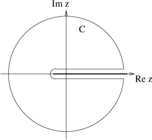
Figure 2: Contour for the integral in the complex $Q$ plane leading to Eq. (13). The thick line on the real axis denotes the cut of the Green function $\hat{T}(Q)$.

To leading order in $1/M$ one has an additional result: since the mass enters only in the combination $q+Mv$, the decay rate for a heavy meson of heavy quark mass $M+\delta M$ is $\Gamma(M+\delta M)\approx\mbox{Im}\hat{T}|_{q=\delta Mv}$. If we define $\hat{T}(Q)=T(Qv,v)$, which depends implicitly on $M$, then to leading order in $M$ the dependence on $M$ and $Q$ is only through the combination $M+Q$. It is straightforward now to use standard methods of analysis to relate an integral of $\Gamma$ to the Green function of complex argument. Using the contour in Fig. 2, we have

$$\left.{1\over(n-1)!}{d^{n-1}\over dz^{n-1}}{\hat{T}(z)\over(z+i\Delta)^{n}}\right|_{z=i\Delta}+\left.{1\over(n-1)!}{d^{n-1}\over dz^{n-1}}{\hat{T}(z)\over(z-i\Delta)^{n}}\right|_{z=-i\Delta}={1\over 2\pi i}\oint dz{\hat{T}(z)\over(z^{2}+\Delta^{2})^{n}}.$$ (13)

The right hand side of this equation is the width calculated to leading order in $1/M$ in the effective theory, $\hat{\Gamma}_{0}$, averaged over masses with a particular weight. We have introduced a parameter $n$, the power of the denominator in (13), to guarantee vanishing of the integral on the circle at infinity. It needs to be adjusted depending on the number of spacetime dimensions. Defining

$$\langle{f(M)}\rangle=\int_{-\infty}^{\infty}dx\;w(x)f(x)$$ (14)

with the weight function defined by

$$w(x)={(n-1)!\over(2n-3)!!}{1\over 2\pi\Delta}\left({2\Delta^{2}\over(x-M)^{2}+\Delta^{2}}\right)^{n},$$ (15)

and recalling that the width vanishes when $m_{B}<m_{D}+m_{\pi}$, we have obtained

$$\langle{\hat{\Gamma}_{0}(M)}\rangle={2^{n-1}\Delta^{2n-1}\over(2n-3)!!}\left\{\left.{d^{n-1}\over dz^{n-1}}{\hat{T}(z)\over(z+i\Delta)^{n}}\right|_{z=i\Delta}+\left.{d^{n-1}\over dz^{n-1}}{\hat{T}(z)\over(z-i\Delta)^{n}}\right|_{z=-i\Delta}\right\}.$$ (16)

This is of the form of our main result, but is not quite complete. It gives a peculiar average over heavy quark mass of the decay width to leading order in $1/M$ in terms of the off-shell effective theory Green function with complex momentum. The right hand side can be evaluated using an operator product expansion if $\Delta$ is large enough. As in the case of semileptonic decaysChay:1990da the leading operator in the expansion is of the form $\bar{h}_{v}\Gamma h_{v}$ and has a normalized matrix element in the state $H(v)$. Since its coefficient is computed perturbatively, one has, to leading order in $1/M$,

$$\langle{\hat{\Gamma}_{0}(M)}\rangle=\langle{\Gamma_{Q}(M)}\rangle$$ (17)

where $\Gamma_{Q}(M)$ is the perturbative width of the heavy quark.

The next term in the operator product expansion of $\hat{T}(i\Delta)$ involves an operator with one derivative, $\bar{h}_{v}\Gamma D_{\mu}h_{v}$, which has vanishing expectation value in the state $H(v)$. Therefore, the leading correction to Eq. (17) from the OPE is of order $1/M^{2}$. However, the Hamiltonian ${\cal H}$ itself has an expansion in $1/M$ so we have yet to establish the validity of quark-hadron duality for the decay width to order $1/M^{2}$. Moreover, the relation between the weak Hamiltonian and its representation in the HQET involves Wilson coefficients that have explicit mass dependence. Both types of correction spoil the invariance $M\to M+\delta M$, $Q\to Q-\delta M$. We address these issues next.

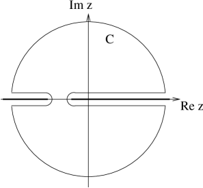
Figure 3: Contour for the integral in the complex $Q$ plane leading to Eq. (22). The thick lines on the real axis denote the cuts in the Green function $\hat{T}_{k}$ and coefficient function $C_{k}$.

The effective Hamiltonian ${\cal H}$ has an HQET expansion in powers of $1/M$,

$${\cal H}=C_{0}\hat{\cal H}_{0}+{1\over M}C_{1}\hat{\cal H}_{1}+\cdots$$ (18)

A sum over several possible operators at each order in $1/M$ is implicit. The coefficients $C_{k}$ are functions of $M/\mu$, where $\mu$ is a renormalization point which we chose to be a fixed number, large enough that the coefficients can be computed perturbatively. We do not set $\mu=M$ since this would introduce additional $M$ dependence into the operators (which are also renormalized at the scale $\mu$). There is a corresponding expansion of the Green function in Eq. (10),

$$T=C_{0}\hat{T}_{0}+{1\over M}C_{1}\hat{T}_{1}+\cdots$$ (19)

and of the width,

$$\Gamma=\hat{\Gamma}_{0}+\hat{\Gamma}_{1}+\cdots$$ (20)

Consider the individual averages

$$\langle{\hat{\Gamma}_{k}(M)}\rangle=\int dQ\;w(Q)\hat{\Gamma}_{k}(Q)$$ (21)

where the weight function $w$ is given in Eq. (15). In order to use a dispersion relation like in (13) we note that the explicit inverse powers of mass give poles at $z=-M$ and the Wilson coefficients, with typical $\ln(M)$ behavior, give cuts extending from $z=-M$ to $-\infty$. Using the contour in Fig. 3, which excludes these cut and pole, we are led to consider

$${1\over 2\pi i}\oint dz\;{C_{k}(z+M)\hat{T}_{k}(z)\over(z+M)^{k}(z^{2}+\Delta^{2})^{n}}=$$ (22)

$$~{}~{}\left.{1\over(n-1)!}{d^{n-1}\over dz^{n-1}}{C_{k}(z+M)\hat{T}_{k}(z)\over(z+M)^{k}(z+i\Delta)^{n}}\right|_{z=i\Delta}+\left.{1\over(n-1)!}{d^{n-1}\over dz^{n-1}}{C_{k}(z+M)\hat{T}_{k}(z)\over(z+M)^{k}(z-i\Delta)^{n}}\right|_{z=-i\Delta}$$

On the other hand, the integral can be written as a sum of two terms, namely, the width average we want and the integral over a contour below and above the cut on the negative real axis. The latter is suppressed by powers of $M$. To estimate it we note that since the Green function $\hat{T}$ is analytic in this region we may simply replace it by a power of the mass given by dimensional analysis, $\hat{T}(z)\sim(z+M)^{p}$ where $p=5$ in four dimensions ($p=2D-3$ in the general case of $D$ dimensions). Also, we may take the Wilson coefficient to be a simple $\log$ for this estimate. Then the integral around the cut is

$${1\over 2\pi i}\int dz {\ln(z+M)(z+M)^{p-k}\over(z^{2}+\Delta^{2})^{n}}$$ (23)

$$= {1\over(n-1)!}{d^{n-1}\over dz^{n-1}}\left[\left.{\ln(z+M)(z+M)^{p-k}\over(z+i\Delta)^{n}}\right|_{z=i\Delta}+(\Delta\to-\Delta)\right]$$

$$= {\cal O}(M^{p-k+1-2n}\ln(M))$$

For comparison, a similar estimate of the average $\langle{\Gamma_{k}(M)}\rangle$ using $\Gamma_{k}(x)\sim x^{p-k}$ gives

$$\int_{0}^{\infty}dx{x^{p-k}\over[(x-M)^{2}+\Delta^{2}]^{n}}={2\pi\over(2\Delta)^{2n-1}}{(2n-2)!\over[(n-1)!]^{2}}M^{p-k}\left(1+{\cal O}({\Delta\over M})\right)$$ (24)

Thus, we can express the width average in terms of the off-shell Green function and derivatives in Eq. (22) up to corrections suppressed by $(\Delta/M)^{2n-1}\ln(M)$.

As in the case of semileptonic decaysChay:1990da , we can now calculate the width average $\langle{\Gamma(M)}\rangle$ by computing the off-shell Green functions using an OPE. But we can do better: we can show that there are no corrections of order $1/M$. As in the case of semileptonic decays, the OPE is an expansion in operators of the form $\bar{h}_{v}\Gamma D^{l}h_{v}$ where $D$ is a covariant derivative. The central observations are that the operator $\bar{\Gamma}h_{v}D_{\mu}h_{v}$ has vanishing expectation valueChay:1990da and the expansion for $\hat{T}_{k}$ starts at order $\bar{h}_{v}\Gamma D^{k}h_{v}$. The latter statement is non-trivial. Consider the case of semileptonic decays. In the original work of Ref. Chay:1990da this question is sidestepped by doing a simultaneous expansion in large momentum transfer (the OPE) and the HQET. But, following Ref. Mannel:1993su , one could first express the Green function in the HQET and only then do the OPE. Although Ref. Mannel:1993su does not consider the effect of subleading operators, it is clear that the two approaches yield the same result only if the OPE of products of subleading operators starts at the corresponding order in $\bar{h}_{v}D^{l}h_{v}$. Clearly, a similar indirect argument applies here, but we know of no direct proof of the statement.

Our main result is then

$$\langle{\Gamma(M)}\rangle=\langle{\Gamma_{Q}(M)}\rangle\left(1+{\cal O}({1\over M^{2}})\right).$$ (25)

It should be noted that the corrections that have been omitted are parametrically small at large $M$, but can be quantitatively large, depending on the values of $M$, $n$ and $\Delta$.

In the ’t Hooft model our result is in agreement with the empirical observations of Ref. Grinstein:2001zq where the averaged widths agree to order $1/M^{2}$ while the un-averaged ones agree at best to order $1/M$. The weight functions used for averages in Ref. Grinstein:2001zq were Gaussian, $w(x)\sim x^{n}\exp(-(x-M)^{2}/\Delta^{2})$. We have checked that the results still hold for the weight function in Eq. (15). It is interesting that substantial duality violation is found if the power $n=1$ is used. In the realistic case of QCD in four dimensions one is left with the very realistic possibility that the physical hadronic width of a heavy meson exhibits oscillations of magnitude $1/M$ about the partonic width which are erased out when performing unphysical mass averages. Some evidence for this was presented in Ref. Altarelli:1996gt where it was observed that the $b$-quark width agrees better with experimental hadronic widths if the quark mass is replaced by the $B$ or $\Lambda_{b}$ masses, respectively, and in Ref. Nussinov:2001zc which argues that the $D^{0}-D_{s}$ lifetime difference is also primarily a phase space effect. In a similar vein, Ref. Colangelo:1997ni shows how $1/M$ violations to local, but not global, duality may occur in $B$-meson correlations.

To summarize, we have shown that the hadronic width of a heavy meson averaged over the heavy quark mass as in Eq. (14) is correctly given by the corresponding average of a perturbative heavy quark width up to corrections of order $1/M^{2}$. This result can be applied to the decay widths of heavy mesons in the ’t Hooft model, and explains the numerical observations of Ref. Grinstein:2001zq . The result, however, is not of direct phenomenological significance since it is impossible to perform mass averages of observed decay widths of $B$ mesons. However, our result adds to the body of evidence that heavy meson widths cannot be reliably computed using perturbation theory, at least not with a precision of order $1/M^{2}$.

- (1) E. D. Bloom and F. J. Gilman, Phys. Rev. D 4, 2901 (1971).
- (2) E. D. Bloom and F. J. Gilman, Phys. Rev. Lett. 25, 1140 (1970).
- (3) E. C. Poggio, H. R. Quinn and S. Weinberg, Phys. Rev. D 13, 1958 (1976).
- (4) K. G. Wilson, Phys. Rev. 179, 1499 (1969)
- (5) C. G. Boyd, B. Grinstein and A. V. Manohar, Phys. Rev. D 54, 2081 (1996) [hep-ph/9511233].
- (6) J. Chay, H. Georgi and B. Grinstein, Phys. Lett. B 247, 399 (1990).
- (7) B. Grinstein and R. F. Lebed, Phys. Rev. D 57, 1366 (1998) [hep-ph/9708396].
- (8) G. ’t Hooft, Nucl. Phys. B 75, 461 (1974).
- (9) B. Grinstein, Phys. Rev. D 64, 094004 (2001) [arXiv:hep-ph/0106205].
- (10) T. Mannel, Nucl. Phys. B 413, 396 (1994) [arXiv:hep-ph/9308262].
- (11) G. Altarelli, G. Martinelli, S. Petrarca and F. Rapuano, Phys. Lett. B 382, 409 (1996) [hep-ph/9604202].
- (12) P. Colangelo, C. A. Dominguez and G. Nardulli, Phys. Lett. B 409, 417 (1997) [hep-ph/9705390].
- (13) S. Nussinov and M. V. Purohit, arXiv:hep-ph/0108272.