Solar Neutrino Zenith Angle Distribution
and Uncertainty in Earth Matter Density

Abstract

We estimate in this paper the errors in the zenith angle distribution for the charged current events of the solar neutrinos caused by the uncertainty of the earth electron density. In the model of PREM with a $5\%$ uncertainty in the earth electron density we numerically calculate the corrections to the correlation between $[N]_{5}/[N]_{2}$ and $[N]_{2}/[N]_{3}$, and find the errors notable.

Forthcoming results from SNO[1] include a measurement of the day-night asymmetry ($A_{DN}$)[2, 3, 4, 5]. This measurement is crucial to confirming the matter conversion solution to the solar neutrino problem. And the analysis on the zenith angle distribution of the events during the night may provide some insights to distinguish the various MSW solutions, i.e. LMA, LOW and SMA[6]. In the calculation of the regenerated $\nu_{e}$ flux, the electron density of the earth matter with which the neutrinos interact is a critical quantity. The uncertainty in Earth-matter density and chemical component can be a major cause of the error in $A_{DN}$ and the zenith angle distribution. So it will be interesting to estimate these errors. Furthermore since the experimental value of the $A_{DN}$ is around $\sim 0.047$[2] and the theoretical expectations on the zenith angle distributions are small in magnitude[6], it is necessary to perform a quantitative estimation on these errors.

In this paper, we follow the procedure outlined in [7] and study the uncertainty in the earth matter density, then investigate its implications on the predictions of $A_{DN}$ and the zenith angle distributions. We quantify the uncertainties of the earth matter in terms of two parameters: one is $\delta N_{e}/N_{e}$, the variation in magnitude of the density which generally is expected to be around a few percent; the second one is $\delta x$ which specifies the limitation on the spacial dimension by geophysics experiments and inverting calculations used in the fit of the earth density models. In general the scale $\delta x$ is not much larger than the neutrino oscillation length, e.g., in the case with the parameters of the favored LMA solution, so its effect might arise beyond the linear order. We will show in this paper that this effect causes an sizable error in the zenith angle distributions.

To begin with we consider a two-neutrino mixing model for simplicity. As discussed in[8, 4] the neutrino can be treated as a incoherent mixture of two mass eigenstates. In the day-time the survival probability for $\nu_{e}$ is given by,

$$P^{D}=P_{1}\cos^{2}\theta+(1-P_{1})\sin^{2}\theta~{},$$ (1)

where the mixing angle is defined through,

$$\nu_{1}=\cos\theta~{}\nu_{e}-\sin\theta~{}\nu_{\mu}~{},~{}\nu_{2}=\sin\theta~{}\nu_{e}+\cos\theta~{}\nu_{\mu}~{},~{}$$ (2)

and $P_{1}$ is the probability of the $\nu_{e}\to\nu_{1}$ conversion inside the sun[9, 6]. During the night time, the presence of the earth matter leads to a zenith angle dependent regeneration of the $\nu_{e}$,

$$P^{N}=P_{1}+(1-2P_{1})P_{2e}=P^{D}-2Xf_{reg}~{},$$ (3)

where $P_{2e}$ is the probability of the $\nu_{2}\to\nu_{e}$ conversion inside the Earth, $X=P_{1}-1/2$. And

$$f_{reg}(\theta_{z})\equiv P_{2e}(earth~{}matter)-P_{2e}(vacuum)~{},$$ (4)

is the regeneration factor which vanishes in the absence of the Earth matter effect. Defining ${\bar{f}}_{reg}$ as the regeneration factor integrated over the zenith angle, one has the day-night asymmetry,

$$A_{DN}\equiv\frac{P^{N}-P^{D}}{\frac{1}{2}(P^{N}+P^{D})}=\frac{-2X{\bar{f}}_{reg}}{0.5+(\cos 2\theta-{\bar{f}}_{reg})X}.$$ (5)

The matter effects has entered the day-night asymmetry through $f_{reg}$. Formally,

$$P_{2e}(E_{\nu},\theta_{z})={{\Big{|}}\cos\theta\lfloor{\cal T}exp\lfloor-i\int_{0}^{D\cos\theta_{z}}H[N^{\theta_{z}}_{e}(x)]dx\rfloor\rfloor_{ee}+\sin\theta\lfloor{\cal T}exp\lfloor-i\int_{0}^{D\cos\theta_{z}}H[N^{\theta_{z}}_{e}(x)]dx\rfloor\rfloor_{e\mu}{\Big{|}}}^{2}~{},$$ (6)

where $D=12742$ is the diameter of the Earth in unit of kilometer and $H[N^{\theta_{z}}_{e}(x)]$ is the effective Hamiltonian for the given trajectory with zenith angle $\theta_{z}$,

$$H[N^{\theta_{z}}_{e}(x)]=\frac{\Delta m^{2}}{4E_{\nu}}\left(\begin{array}[]{cc}2\sin^{2}\theta&\sin 2\theta\\ \sin 2\theta&2\cos^{2}\theta\end{array}\right)+\left(\begin{array}[]{ccc}\sqrt{2}G_{F}N^{\theta_{z}}_{e}(x)&0\\ 0&0\end{array}\right).$$ (7)

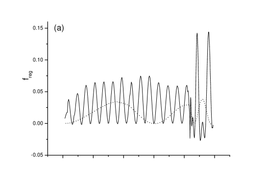
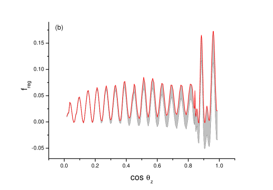
Figure 1: Plot of the regeneration factor vs the zenith angles for neutrino energy at 11 MeV. The Earth matter model of PREM and the neutrino oscillation parameters in Eq.(8) have been used. (a) The solid line is for LMA while the dotted line for LOW. (b) the error bars corresponds to the corrections due to the $5\%$ uncertainty in the matter density ( PREM ) . The fluctuation in LOW case is smaller than the LMA case, so we have not shown them explicitly in this figure.

In Eq.(7), $N^{\theta_{z}}_{e}(x)$ is the Earth Electron Density (EeD) along the trajectory of the zenith angle $\theta_{z}$. If the density is known, the regeneration factor $f_{reg}=P_{2e}-\sin^{2}\theta$ can be calculated accurately. As an example we take the Preliminary Reference Earth Model (PREM)[10] and plot in Fig.1.(a) the regeneration factor as a function of the zenith angle. In the numerical calculation we take the neutrino energy to be 11 MeV and the oscillation parameters to be[11]

$$LMA~{}:~{}\Delta m_{12}=3.7\times{10}^{-5},\tan^{2}\theta=0.37~{},$$

$$LOW~{}:~{}\Delta m_{12}=1.0\times{10}^{-7},\tan^{2}\theta=0.67$$ (8)

One can see from this figure that the regeneration factors oscillate periodically with certain lengths. And different oscillation lengths correspond to different MSW solutions.

Given the parameters in Eq.(8) and the standard solar density[12], we follow [6, 9] and obtain numerically that $\cos 2\theta_{S}\approx-1$ and $P_{c}\approx 0$, which can be used to get the $\nu_{e}\to\nu_{1}$ conversion in the Sun. Fluctuations in the solar density will affect $P_{1}$, consequently also influence the MSW solutions[13]. In that situation a variance of $P^{D}$ has been defined to estimate the relevant error [14]. In this paper, however, we concentrate on the errors caused by the uncertainty of EeD.

The EeD available today, is known only to some certain precision [15, 16]. As to PREM, significant uncertainties due to the local variation have been documented[17]. Quantitatively its precision is roughly $5\%$ averaged per spherical shell with thickness of 100 Km or so [18]. The uncertainties of the Earth matter density cause errors in the calculation of the $\nu_{e}$ survival probability during the night time. In the following we study numerically the uncertainties in the solar neutrino zenith angle distributions.

As described detailly in [7], we introduce a weighted average over the whole sample space of possible earth density profile. Denoting the averaged earth density function, such as the widely used PREM by $\hat{N_{e}}(x)$, we have $\hat{N}_{e}(x)=<N_{e}(x)>=\int[DN_{e}]F[N_{e}(x),x][{\cal D}N_{e}]$ where $F[N_{e}(x),x][{\cal D}N_{e}]$ is the probability of obtaining the EeD $N_{e}(x)$ in the neighborhood of x,

$$F[N_{e}(x),x]=\frac{1}{N_{e}(x)\sqrt{2\pi}s(x)}exp\{-\ln^{2}\lfloor~{}N_{e}(x)/N_{0}(x)~{}\rfloor/\lceil 2s^{2}(x)\rceil\},$$

$$s(x)=\sqrt{\ln\lceil 1+r^{2}(x)~{}\rceil},~{}~{}N_{0}(x)={\hat{N}}_{e}(x)exp\lfloor-s^{2}(x)/2~{}~{}\rfloor,$$ (9)

where $r(x)=\sigma(x)/{\hat{N}}_{e}(x)$ characterizes the precision of the earth electron density.

The averaged value and the variance of the $\nu_{2}\to\nu_{e}$ conversion probability can be written now separately as,

$$<P_{2e}(E_{\nu},\theta_{z})> \equiv \int P_{2e}(\theta_{z})F[N^{\theta_{z}}_{e}(x)][{\cal D}N^{\theta_{z}}_{e}]~{}$$

$$= \lim_{I\to\infty}\int\prod_{i=1}^{I}F[N^{\theta_{z}}_{e}(x_{i}),x_{i}]dN^{\theta_{z}}_{e}(x_{i})\times$$

$$~{}~{}~{}~{}~{}P_{2e}(\theta_{z})[\{N^{\theta_{z}}_{e}(x_{1}),...N^{\theta_{z}}_{e}(x_{i}),...N^{\theta_{z}}_{e}(x_{I})\}]$$

$$= \lim_{K\to\infty}K^{-1}\sum_{k=1}^{K}{\tilde{P}_{k}}(N^{(k)}_{e}),$$

$$\delta f_{reg} = \delta P_{2e}(E_{\nu},\theta_{z})\equiv\sqrt{<P^{2}_{2e}(E_{\nu},\theta_{z})>-{<P_{2e}(E_{\nu},\theta_{z})>}^{2}}$$ (10)

$$= {[\lim_{K\to\infty}{(K-1)}^{-1}\sum_{k=1}^{K}{{\big{(}}{\tilde{P}_{k}}-<P_{2e}>{\big{)}}}^{2}]}^{1/2}.$$

We evaluate the functional integrations in Eq.(10) using a method similar to that of the lattice gauge theory. In the numerical calculation we discretize the neutrino path into I bins, $\delta x_{i}$ (i = 1, 2, …I) and in the i-th bin the EeD function $N_{e}(x)$ is given by Eq.(9). Furthermore we have replaced the functional integration over the EeD by a sum over K arrays, $N^{(k)}_{e}$ k=1, 2, …K. In Eq.(10) ${\tilde{P}}_{k}$ is the conversion probability evaluated with the $k^{\prime}th$ density profile $N^{(k)}_{e}$ . As to PREM each point in the array $N^{(k)}_{e}$ which consists of $N_{e}(x_{1}),....N_{e}(x_{i}),....N_{e}(x_{I})$ is generated from PREM weighted with a Gaussian-like logarithm distribution. Since the deviation from PREM due to local variation is roughly $5\%$ and the deviation is averaged per spherical shell with thickness of 100 Km, we take $r=5\%$ and choose the bin sizes $\delta x_{i}$ to be the distance the neutrino travels along the path of zenith angle $\theta_{z}$ within a spherical shell of thickness 100 Km. So in general $\delta x_{i}$ will not be equal except for $\theta_{z}=0$.

We note that the EeD uncertainty scale $\delta x$ differs from the one, $l_{\rho}=\rho/{d\rho\over dx}$ considered in [6] to characterize the flatness (adiabaticity) of the density profile. Both of these scales are important to the studies on the neutrino oscillations in matter. The effects of the $l_{\rho}$ can be taken into account in the exact numerical calculation, however to reduce the error caused by $\delta x$ a more precise density profile is needed. Especially when $\delta x$ is comparable to the neutrino oscillation length in matter, one has to be careful in estimating the errors for oscillation probability.

In Fig.1.(b) we plot $\delta f_{reg}$ and $f_{reg}$ as a function of the zenith angle. One can see from this figure that LMA suffers a larger error. For LOW the error is roughly two percent and for SMA the error is much smaller. So we have not shown them in the figure. Integrated over the zenith angle, it gives rise to a correction of $20\%$ roughly to the $A_{DN}$ for LMA, however the corrections are small for LOW and SMA. Combined with Fig.1.(a), we see that the errors are small so that $A_{DN}^{LMA}$ and $A_{DN}^{LOW}$ can be distinguished.

To see the effects on the solar neutrino observations, we now estimate the errors in the rate of the charged current events during the night time. Following [6] we define the normalized rate of the charged current events as,

$$[CC](\theta_{z}) \equiv N_{CC}/N^{SSM}_{CC}$$ (11)

$$= \int_{E_{th}}dT_{e}\int_{E_{\nu}}dE_{\nu}P^{N}(E_{\nu},\theta_{z})\Phi(E_{\nu})\int dT^{{}^{\prime}}d\cos\theta_{L}{\hat{\sigma}}(E_{\nu},T^{{}^{\prime}},\cos\theta_{L})R(T_{e},T^{{}^{\prime}})/N^{SSM}_{CC}$$

$$= \int_{E^{0}_{\nu}}dE_{\nu}\Phi(E_{\nu})P^{N}(E_{\nu},\theta_{z})\sigma_{CC}(E_{\nu})/N^{SSM}_{CC}~{}~{},$$

where $\Phi(E_{\nu})$ contains both the neutrino flux from the Boron decay and the $He+P$ chain in the sun[19, 5], and $N^{SSM}_{CC}$ is the normalization factor which equals to the integral in $r.h.s.$ taken at $P^{N}=1$. From the 2’nd to the 3’rd line of Eq.(11), the integration of the differential cross section ${\hat{\sigma}}$ with respect to the recoil electron kinetics $T_{e}$ and the scatting angle $\theta_{L}$ has been replaced by a total charged current cross section ${\sigma}_{CC}$ of the neutrino on the Deuteron, since the possible uncertainty from $T_{e},~{}\theta_{L}$ can be canceled in the $[CC]$ as a ratio of $N_{CC}$ to $N_{CC}^{SSM}$. The $E_{\nu}$ dependence in ${\sigma}_{CC}$ is accessed by employing a quick function from interpolation in [20]. The starting point of the neutrino energy is set at $E^{0}_{\nu}\approx Q+E_{th}$, with $Q=1.442MeV$ being the deuterium threshold energy and $E_{th}=5MeV$ the electron threshold energy. In Fig.2, we plot the zenith angle distribution of the charged current events rate in Eq.(11). One can see that the SNO charged current data lies in the middle between the LMA and LOW. This serves also as a check of our numerical calculation. Following the binning method of [6], we plot in Fig.3.(a) and Fig.3.(b) the charged current events v.s. bins (note for the fifth bin $\cos\theta_{z}\sim(0.83,~{}0.92)$ in the case of SNO), which shows that,

$$LMA~{}:~{}[N]_{1}<[N]_{2}\leq[N]_{3}\leq[N]_{4}\leq[N]_{5},$$

$$LOW~{}:~{}[N]_{2}\geq[N]_{4}>[N]_{1}\sim[N]_{3}>[D].$$ (12)

Quantitatively, it reads, $[N]_{5}/[N]_{2}=0.999\approx 1$ and $[N]_{2}/[N]_{3}=0.995\approx 1$ for LMA while $[N]_{5}/[N]_{2}=0.982,[N]_{2}/[N]_{3}=1.053$ for LOW, from which it might be possible to distinguish LMA from LOW. The calculation for SMA can be easily worked out, however for simplicity we will not repeat it here.

Making use of Eqs.(11), (10), and (3) we estimate the errors in the charged current events rate caused by the uncertainties in the earth electron density

$$\delta[CC]\propto\int_{E^{0}_{\nu}}dE_{\nu}\Phi(E_{\nu})(-2X\delta f_{reg})\sigma_{CC}(E_{\nu}),$$ (13)

which we show in Fig.(4) by the error-bars. To avoid multi-fold integration which is a computer time consuming, we investigate $\delta f_{reg}$ at neutrino energies of $8,10,11,12$ MeV and find the results almost unchanged. To be conservative we have used the maximal value for $\delta f_{reg}$.

We see from the figure that the errors become larger as the zenith angle increases in the case of LMA. Averaged over bins we have $([N]_{5}-\delta[N]_{5})/[N]_{2}\approx 0.935$ while $([N]_{2}+\delta[N]_{2})/([N]_{3}-\delta[N]_{3})\approx 1.043$. As indicated in the figures 13-16 of [6] that the LMA sheet in their correlation figures mainly stretched along the $A_{DN}$ direction, we study a correlation between $[N]_{5}/[N]_{2}$ and $[N]_{2}/[N]_{3}$, which we show in Fig.5. One sees that the point ($1,~{}1$) for LMA is swollen into a rectangle close to the point ( $0.982,1.053$ ) for LOW. In this figure we have not shown the error bars for LOW since they are small.

So far the precision of PREM which we assume is $5\%$. Certainly errors on the zenith angle distribution become larger if the uncertainty in the earth electron density is bigger. Sure a modern Earth’s density model with higher precision will reduce the errors considered in this paper. As an example we take density model AK135[21]. The precision of AK135 is widely considered to be about $1\sim 2\%$, and its uncertainty scale is roughly $\delta x\approx 50$ Km since the model was presented in a data table. Taking a $2\%$ uncertainty in the electron density we show our results in Figure. 6. one finds $([N]_{5}-\delta[N]_{5})/([N]_{2}+\delta[N]_{2})\approx 1.033$ while $([N]_{2}+\delta[N]_{2})/([N]_{3}-\delta[N]_{3})\approx 1.017$. From Fig.6.(b), we see the gap between LMA and LOW enlarged. This makes it easier to distinguish the LMA from LOW than the prediction from PREM.

In summary, we have estimated in this paper the errors in the zenith angle distribution of the charged current event rates of the solar neutrinos originated from the electron density uncertainty. Our results show that the corrections are not significant in the case of LOW and SMA, however, error is notable for LMA. Even though our estimations are given for specific parameters and qualitatively, the results of this paper indicate that to observe the zenith angle distribution a precise knowledge on the Earth electron density is necessary.

The work is supported in part by the NSF of China under Grant No 19925523 and also supported by the Ministry of Science and Technology of China under Grant No NKBRSF G19990754.

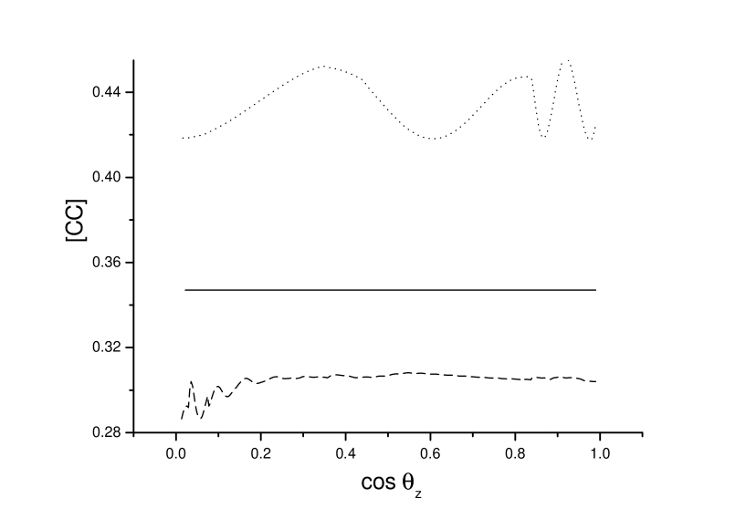
Figure 2: Charged current event rates vs the zenith angles. The dotted line is for LOW and the dashed line for LMA. The solid straight line is the data of the SNO observation.

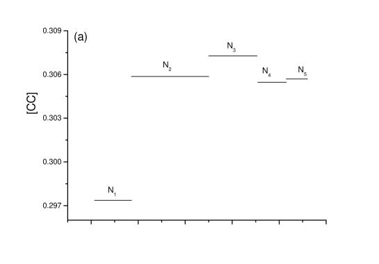
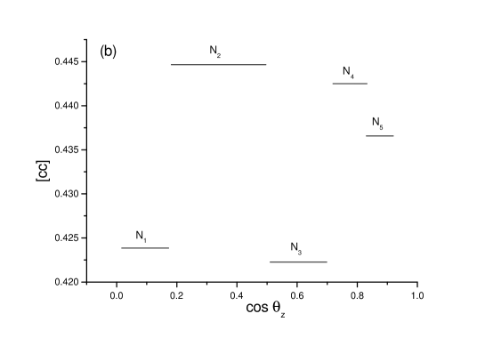
Figure 3: Plot of the charged current event rates averaged over bins as a function of the zenith angles. (a) is for LMA which corresponds to the dashed line in Fig.2, (b) is for LOW corresponding to the dotted line in Fig.2.

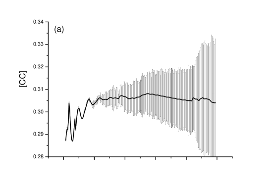
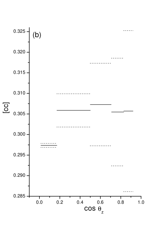
Figure 4: Plot of the errors in the charged current event rates for LMA vs the zenith angles. (a) shows the error-bars attached on the dashed line of Fig.2. (b) The solid line is the same as that in Fig.3(a). And between the dotted lines are the errors caused by the uncertainty in the electron density.

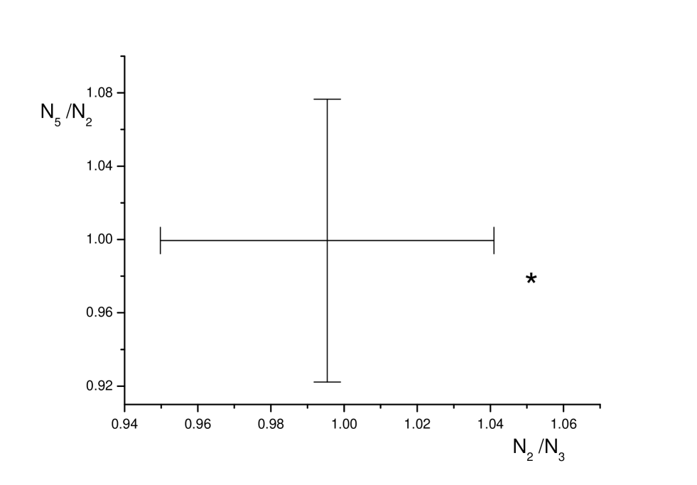
Figure 5: Plot of the correlation between $N_{5}/N_{2}$ and $N_{2}/N_{3}$ . The center of the cross corresponds to the best-fit LMA, the star is for the best-fit LOW . The error bars ( cross ) span a rectangle and indicate a possible blur due to the uncertainty of EeD.

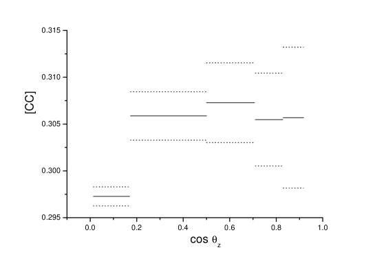
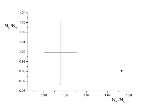
Figure 6: (a) is the same as Fig.4.(b), but with a $2\%$ EeD uncertainty in the AK135 model. (b) the same as Fig.5. but with AK135 instead of PREM.

References

• [1] Q.R.Ahmad et al., SNO Coll. , nucl-exp/0106015
• [2] Super-Kamiokande Collaborattion, hep-ex/9812009, or Phys.Rev.Lett. 82 (1999) 1810
• [3] A.J.Baltz and J.Weneser, Phys.Rew.D35(87) 528 ; 37(88) 3364 ; G.L.Fogli et.al., IASSNS-AST 96/21 ; J.N.Bachall, P.I.Krastev and A.Yu.Smirnov, Phys.Rev.D 60 (1999)093001
• [4] E.Lisi and D. Montanio, P.R.D 56 ( 1997 ) 1792
• [5] G.L.Fogli et al., hep-ph/0008012 V.Barger et.al., hep-ph/0104095
• [6] M.C.Gonzalez-Garcia et al., hep-ph/00012313 ;
• [7] Lian-You Shan, Bing-Lin Young and XinMin Zhang, hep-ph/0110414
• [8] A.S.Dighe, Q.Y.Liu, A.Yu.Smirnov, hep-ph/9903329
• [9] S.T.Petcov, Theory of Neutino Oscillations, 6’th School on Non-accelerator Astroparticle Physics, July 2001, ICTP, Trieste
• [10] A.M.Dziewonsky and D.L.Andson , Phys.Earth.Planet. Inter 25(1981) 297
• [11] D. Marfatia, V.Barger an K. Whisnant, hep-ph/0106207 ; P.I.Krastev and A.Yu. Smirnov , hep-ph/0108177 ; J.N.Bachall et.al, hep-ph/0111150
• [12] Electron density distribution is available at the website of J.N. Bahcall.
• [13] F.N.Loreti and A.B.Balantenkin, Phys. Rev. D (1994) 4762; H. Nunokawa et al. Nucl.Phys. B 472 (1996) 495; C.P. Burgess and D. Michaud, Ann. Phys. NY, 256 (1997) 1
• [14] A.B.Balantenkin et.al, Phys.Rev.D 54 ( 1996 ) 3941
• [15] B.Jacobsson et.al, hep-ph/0112138
• [16] R.J.Geller and T.Hara, hep-ph/0111342
• [17] R. Jeanlow and S. Morris, Ann Rev. Earth Plan. Sci 14 (1986)377 ; R. Jeanlow Ann Rev. Earth Plan. Sci 18 ( 1990 ) 357; Fu-Tian Liu et al, Geophys. J. Int. 101 (1990) 379; T.P. Yegorova et.,al., Geophys. J. Int, 132 ( 1998 ) 283; B. Romanowicz, Geophys. Res. Lett., 28 ( 2001) 1107.
• [18] B.A.Bolt, Q.J.R.astr.Soc 32 (1991) 367
• [19] J.N. Bahcall et.al., Phys. Rev. C. 54 ( 1994 ) 411 ; Phys. Rev. D, 56 (1997)3391
• [20] J.N.Bahcall and E.Lisi, Phys. Rev. D 54 ( 1996) 5417
• [21] Kennett B.L.N., et.al , Geophysics.J.Int, 122(1995) 108, Montagner J.P. et.al, Geophysics.J.Int, 125(1995) 229
Refer to caption
Refer to caption