KOBE-TH-01-08

Stability and experimental flux bound of Fermi Ball

Kenzo Ogure

Department of Physics, Kobe University,
Rokkoudaicho 1-1, Nada-Ku, Kobe 667-8501, Japan

and

Jiro Arafune

National Institution for Academic Degrees,
Hitotsubashi 2-1-2, Chiyoda-Ku, Tokyo 101-8438, Japan

Takufumi Yoshida

Department of Physics, Tokyo University,
Hongo 7-3-1, Bunkyo-Ku, Tokyo 113-0033, Japan

We investigate the stability of an Fermi ball(F-ball) within the next-to-leading order approximation in the thin wall expansion. We find out that an F-ball is unstable in case that it is electrically neutral. We then find out that an electrically charged F-ball is metastable in some parameter range. We lastly discuss the allowed region of parameters of an F-ball, taking into account the stability of an F-ball and results of experiments.

PRESENTED AT

COSMO-01
Rovaniemi, Finland,
August 29 – September 4, 2001

1 Introduction

Fermi ball(F-ball), which is a kind of nontopological solitons, is first proposed as a candidate for cold dark matter(CDM) [1]. Similar object is considered to have possibility to explain the baryon number asymmetry of the present universe [2]. An F-ball consists of a closed domain wall and fermions which localize on the wall. Such an object is thought to be produced after a phase transition, in which two almost degenerate vacua exist. At this phase transition, two regions, which correspond to two vacua, and domain walls are produced. If these two vacua are completely degenerate, the domain walls will dominate the energy density of the universe soon [3]. However, if the energy density of one vacuum is slightly smaller than the other one, the true vacuum pushes the domain walls and reduces the false vacuum region. If some fermions are captured on the domain walls, the left region may be stabilized due to the Fermi pressure of the captured fermions.

We first assume that the region has complete spherical form with radius, $R$. In this case, the total energy of this system consists of three parts, the surface, the volume, and the Fermi energy within the thin wall approximation:

$$E_{total}=E_{s}+E_{v}+E_{F}=4\pi R^{2}\Sigma+\frac{4\pi R^{3}\epsilon}{3}+\frac{2N^{\frac{3}{2}}}{3R}.$$ (1)

Here, $\Sigma$, $\epsilon$, and $N$ are the surface tension, the energy density difference between the two vacua, and the number of fermions on the wall, respectively. Since the surface energy and the volume energy are the increasing functions of the radius and the Fermi energy is the decreasing one, this object is stabilized at a certain radius. We deal the volume energy as a perturbation term hereafter, since it is much smaller than the other energies in most cases. Minimizing this total energy with respect to $R$, we find out that it is proportional to the number of the fermions on the wall with the following critical radius, $R_{c}$:

$$E_{total}=\frac{1}{3}\kappa N,\ \ \ (R_{c}=\frac{\sqrt{N}}{\kappa},\ \kappa\equiv(12\pi\Sigma)^{\frac{1}{3}}).$$ (2)

This object is called as Fermi ball.

If this large F-ball were stable, it were interesting as a candidate for CDM. It, however, is unstable against deformation from spherical shape and fragments into small pieces [1]. This can be understood as follows. Since the energy of an F-ball is proportional to the number of the fermions on the wall as above, it has same energy even if it is divided into some smaller F-balls. However, there exists the small volume energy, which we neglected. Taking into account this contribution, we can easily find out that the fragmented state has smaller energy. An F-ball therefore continues to be small until the thickness of the wall becomes comparable to its radius and the thin wall approximation breaks down. Such an F-ball is too small and there must be large number of them in order that they have sizable contribution to CDM. An F-ball was, therefore, thought to consist of a domain wall and a fermion which interact with ordinary matter only very weakly [1].

An electrically charged F-ball, which is stable against the fragmentation owing to the long range electric force, is then proposed [2]. This F-ball can be large and heavy enough to have sizable contribution to CDM even if they are very dilute.

We, however, have three questions about the above treatments of an F-ball:

• Is an electrically neutral F-ball unstable even if the curvature effect is taking into account?

• Is an electrically charged F-ball really stable?

• Is an electrically charged F-ball stable even in the hot early universe where the F-ball is consider to be produced?

First, when we consider an electrically neutral F-ball, we used the thin wall approximation and neglected the contribution from the curvature of the wall. Though this contribution is really much smaller than the total energy of an F-ball, it can be very important. Neglecting the curvature effect, we concluded that the energy of an F-ball is same as that of its fragmented state in the absence of the volume energy. However, if we take into account the contribution from the curvature, two states will have different energies. This curvature contribution, therefore, would determine which state is stable.

Second, The total energy of an electrically charged F-ball approximately consists of the surface energy and the coulomb energy for large $N$ because the coulomb energy is proportional to $N^{2}$:

$$E_{total}\simeq E_{s}+E_{c}=4\pi R^{2}\Sigma+\frac{\alpha N^{2}}{2R}.$$ (3)

Minimizing the total energy with respect to the radius, we obtain the total energy as follows:

$$E_{total}=\frac{1}{3}\kappa(\frac{3\alpha}{4})^{\frac{2}{3}}N^{\frac{4}{3}},\ \ \ (R_{c}=\kappa(\frac{3\alpha}{4})^{\frac{1}{3}}N^{\frac{2}{3}}).$$ (4)

Since the total energy is proportional to $N^{\frac{4}{3}}$, a fragmented state has apparently smaller energy than an F-ball. We therefore can not conclude that the electric force stabilize the F-ball from the fragmentation only by comparing the energies of the two states. We then should investigate that is there any energy barrier to deform an F-ball to a fragmented state. If there is enough barrier due to the electric long range force, an F-ball can be metastable.

Third, in thermal bath, the electric long range force becomes short range one with typical Debye screening length. The energy barrier, which arises from the electric long range force, would become week or disappear due to this Debye screening.

To answer these three questions is the main aim of the present paper. Details of the following analysis are shown in Ref.[4].

2 Stability of a neutral F-ball

We first consider the curvature effect to the stability of an F-ball. Though we only consider a simple model described by the following Lagrangian density, most results will be able to be applied to more complicated models [1]:

$${\cal L}=\frac{1}{2}(\partial_{\mu}\phi)^{2}+\bar{\psi}_{F}(i\gamma^{\mu}\partial_{\mu}-G\phi)\psi_{F}-U(\phi)~{},$$ (5)

where $\phi$ and $\psi_{F}$ are a scalar and a fermion field, respectively, and $G$ is a Yukawa coupling constant. Here, $U(\phi)$ is an approximate double-well potential ,

$$U(\phi)=\frac{\lambda}{8}\left(\phi^{2}-v^{2}\right)^{2}+U_{\epsilon}(\phi)~{},$$ (6)

taking the second term, which breaks $Z_{2}$ symmetry under $\phi\leftrightarrow-\phi$, much smaller than the first one. This model has a kink solution, which interpolates the two vacua, $\phi=v,-v$:

$$\phi(z)=v\tanh{\frac{z-z_{0}}{\delta_{N}}}~{},\ \ \ \ (\delta_{N}\equiv 2/(\sqrt{\lambda}v)).$$ (7)

We assume the width of the wall, $\delta_{N}$ is much smaller than the F-ball size. We call the plane where $\phi$ vanishes ”surface” of the domain wall in the present paper. This domain wall has the surface tension, $\Sigma$:

$$\Sigma=\frac{2\sqrt{\lambda}}{3}v^{3}.$$ (8)

Substituting Eq.(7) into the Euler-Lagrange equation of $\psi_{F}$, we find that $\psi_{F}$ has a zero-mode solution,

$$\psi_{F}(z)=\psi_{F}(z_{0})\exp{\left\{-G\int_{z_{0}}^{z}\mbox{d}z^{\prime}~{}\phi(z^{\prime})\right\}}~{}.$$ (9)

Here, $\psi_{F}(z_{0})$ is a spinor eigenstate of $i\gamma_{3}=-1$. A fermion can localize on the domain wall owing to this zero mode. This model is therefore a suitable model to investigate the properties of an F-ball, since it has the domain wall solution and the fermion, which can localize on the wall.

We evaluate the next-to-leading order approximation of the thin wall expansion in this model. We assume that the scalar field expectation value does not change along the surface and write the surface energy as follows:

$$E_{s}[\phi] = \int\mbox{d}^{3}{\bf x}~{}\left\{\frac{1}{2}(\nabla\phi({\bf x}))^{2}+\frac{\lambda}{8}\left(\phi({\bf x})^{2}-v^{2}\right)^{2}\right\}$$ (10)

$$\sim \int\mbox{d}\theta_{1}\mbox{d}\theta_{2}\mbox{d}w~{}(R_{1}+w)(R_{2}+w)\left\{\frac{1}{2}\dot{\phi}^{2}+\frac{\lambda}{8}\left(\phi^{2}-v^{2}\right)^{2}\right\}~{}$$

$$= \int\mbox{d}S\mbox{d}w~{}(1+\frac{w}{R_{1}})(1+\frac{w}{R_{2}})\left\{\frac{1}{2}\dot{\phi}^{2}+\frac{\lambda}{8}\left(\phi^{2}-v^{2}\right)^{2}\right\}~{},$$ (11)

where $\dot{\phi}$ stands for the derivative of $\phi$ with respect to $w$. The local coordinate, $w$ is perpendicular to the surface and becomes zero on the surface. The curvature radiuses, $R_{1}$ and $R_{2}$ are principle curvature radiuses on each points and the local coordinates, $\theta_{1}$ and $\theta_{2}$ are the corresponding angular coordinates (see Fig.1).

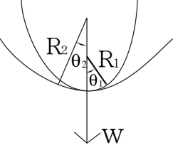
Figure 1: Local coordinates on the wall.

Taking variation of $E_{N}$ with respect to $\phi$, we obtain the equation,

$$\ddot{\phi}+\left(\frac{1}{R_{1}+w}+\frac{1}{R_{2}+w}\right)\dot{\phi}=\frac{\lambda}{2}\phi(\phi^{2}-v^{2}),$$ (12)

with the boundary condition,

$$\phi=\left\{\begin{array}[]{ll}\pm v&(w\rightarrow\pm\infty)\\ 0&(w=0)~{}~{}~{}.\end{array}\right.$$ (15)

We now estimate $E_{s}$ within the thin-wall approximation, ignoring the curvature effect. The equation (12) becomes in the leading order as,

$$\ddot{\phi_{0}}=\frac{\lambda}{2}\phi_{0}(\phi_{0}^{2}-v^{2}),$$ (16)

with the boundary condition,

$$\phi_{0}=\left\{\begin{array}[]{ll}\pm v&(w\rightarrow\pm\infty)\\ 0&(w=0)~{}~{}~{}.\end{array}\right.$$ (19)

The solution to Eq.(16) is the kink,

$$\phi_{0}(w)=v\tanh{\frac{w}{\delta_{N}}}~{}.$$ (20)

Adding the Fermi energy, we obtain the total energy of the neutral F-ball within the thin wall approximation, $E_{N}^{0}$:

$$E_{N}^{0}=\Sigma S+\frac{4\sqrt{\pi}}{3}\int\mbox{d}S~{}n_{F}^{3/2}({\bf x}_{F})~{},$$ (21)

where $\Sigma$ is the surface tension in Eq.(8). We should minimize this total energy, keeping the total fermion number,

$$N=\int\mbox{d}S~{}n_{F}({\bf x}_{F})~{},$$ (22)

constant. Using the Lagrange’s multiplier method, we find that $n_{F}({\bf x}_{F})$ is constant:

$$n_{F}({\bf x}_{F})=\frac{N}{S}~{}.$$ (23)

From this, we finally get the total energy:

$$E_{N}^{0}=\Sigma S+\frac{4\sqrt{\pi}N^{3/2}}{3\sqrt{S}}~{}.$$ (24)

Minimizing with respect to $S$, we obtain,

$$E_{N}^{0}=(12\pi\Sigma)^{1/3}N~{},$$ (25)

with the critical area of the surface,

$$S=\left(\frac{2\sqrt{\pi}}{3\Sigma}\right)^{2/3}N~{}.$$ (26)

Since the total energy is proportional to the number of the fermion, we can not know the stability of the F-ball in this order approximation.

We then calculate the next-to-leading order approximation of the thin wall expansion. We here expand $\phi$ and $E_{N}$ with respect to $\delta_{N}/R_{1}$ and $\delta_{N}/R_{2}$,

$$\phi = \phi_{0}+\phi_{1}+\cdots$$

$$E_{N} = E_{N}^{0}+E_{N}^{1}+E_{N}^{2}+\cdots~{}.$$ (27)

Since $E_{N}^{1}$ vanishes owing to the variational principal, we estimate the energy up to $E_{N}^{2}$. It is enough to expand $\phi$ up to $\phi_{1}$ in this case. From Eq.(12), $\phi_{1}$ satisfies,

$$\ddot{\phi_{1}}-\frac{\lambda}{2}\left(3\phi_{0}^{2}-v^{2}\right)\dot{\phi_{1}}=-\left(\frac{1}{R_{1}}+\frac{1}{R_{2}}\right)\dot{\phi_{0}},$$ (28)

with the boundary condition,

$$\phi_{1}=\left\{\begin{array}[]{ll}0&(w\rightarrow\pm\infty)\\ 0&(w=0)~{}~{}~{}.\end{array}\right.$$ (31)

The solution to Eq.(28) is,

$$\phi_{1}(w)=\frac{1}{2\sqrt{\lambda}}\left(\frac{1}{R_{1}}+\frac{1}{R_{2}}\right)f_{1}(w/\delta_{N})~{},$$ (32)

with,

$$f_{1}(x) = \mbox{sech}^{2}x-\cosh^{2}{x}+\frac{1}{3}\mbox{sinh}^{2}x\mbox{tanh}^{2}x$$ (33)

$$+\frac{\mbox{sech}^{2}x}{12}\left|\sinh{4x}+8\sinh{2x}+12x\right|~{}.$$

Substituting $\phi_{0}$ and $\phi_{1}$ into $E_{N}$, we obtain,

$$E_{N}^{2}=C_{N}^{1}\int\mbox{d}S~{}\frac{1}{R_{1}R_{2}}+C_{N}^{2}\int\mbox{d}S\left(\frac{1}{R_{1}}-\frac{1}{R_{2}}\right)^{2}~{},$$ (34)

with,

$$C_{N}^{1} = \frac{1}{\sqrt{\lambda}}\int\mbox{d}w~{}\left(\sqrt{\lambda}w^{2}\dot{\phi_{0}}^{2}-\dot{\phi_{0}}f_{1}\right)\simeq-\frac{0.25v}{\sqrt{\lambda}}<0$$

$$C_{N}^{2} = -\frac{1}{4\sqrt{\lambda}}\int\mbox{d}w~{}\dot{\phi_{0}}f_{1}\simeq-\frac{0.28v}{\sqrt{\lambda}}~{}<0.$$ (35)

We consider the stability against the fragmentation from the next-to-leading order contribution, $E_{N}^{2}$. The first term in Eq.(34) is proportional to the integration of Gaussian curvature on the closed surface, which is known to be $4\pi$ (Gauss-Bonnet’s Theorem). We therefore find out that the first term does not depend on the shape of the F-ball and depend only on the number of the F-ball. Since $C_{N}^{1}$ is negative, a fragmented state has smaller energy. On the other hand, the second term is zero only for sphere and negative for any other shapes. A spherical F-ball then deforms and fragments to small pieces. We conclude that a neutral F-ball is unstable even in the absence of the volume energy due to the curvature effect.

3 Stability of an electrically charged F-ball

We consider the stability of an electrically charged F-ball in thermal bath in the present section. We here consider the free energy of the fermion gas on the wall and the electron gas, which surrounds the F-ball:

$$F_{C}[V_{e}] = \int\mbox{d}^{3}{\bf x}~{}\left\{-\frac{1}{2e^{2}}\left(\nabla V_{e}({\bf x})\right)^{2}+{\cal F}_{e}(V_{e}({\bf x}))\right.$$ (36)

$$\hskip 56.9055pt\left.\frac{}{}-n_{F}({\bf x}_{F})V_{e}({\bf x})\delta(|{\bf x}-{\bf x}_{F}|)\right\}~{},$$

where ${\cal F}_{e}$ is the free energy density of the electron gas. When the temperature, $T$ is much higher than the electron mass, ${\cal F}_{e}$ can be written as,

$${\cal F}_{e}(V_{e}) = -\frac{2T}{(2\pi)^{3}}\int\mbox{d}^{3}{\bf p}~{}\left\{\frac{p}{T}+\log{\left(1+e^{-\frac{p-V_{e}}{T}}\right)}\right.$$ (37)

$$\hskip 85.35826pt\left.+\log{\left(1+e^{-\frac{p+V_{e}}{T}}\right)}\right\}$$

$$= -\frac{T^{2}V_{e}^{2}}{6}-\frac{V_{e}^{4}}{12\pi^{2}}+(V_{e}\ independent\ terms).$$

The free energy can be obtained by extremizing Eq.(36) with respect to $V_{e}({\bf x})$. Since $V_{e}({\bf x})$ is expected to change rapidly near the wall, we also use the thin wall expansion here. Assuming that $V_{e}$ depends only on $w$, we can express $F_{C}$ as,

$$F_{C}[V_{e}] = \int\mbox{d}S\mbox{d}w~{}(1+\frac{w}{R_{1}})(1+\frac{w}{R_{2}})\left\{-\frac{1}{2e^{2}}\dot{V_{e}}^{2}-\frac{T^{2}V_{e}^{2}}{6}\right.$$ (38)

$$\hskip 85.35826pt\left.-\frac{V_{e}^{4}}{12\pi^{2}}-n_{F}V_{e}\delta(w)\right\}~{}.$$

Taking variation of Eq.(38) with respect to $w$, we obtain the equation,

$$\frac{1}{e^{2}}\ddot{V_{e}}+\frac{1}{e^{2}}\left(\frac{1}{R_{1}+w}+\frac{1}{R_{2}+w}\right)\dot{V_{e}}=\frac{T^{2}V_{e}}{3}+\frac{V_{e}^{3}}{3\pi^{2}}+n_{F}\delta(w)~{},$$ (39)

with the boundary condition,

$$V_{e}\rightarrow 0\hskip 28.45274pt(w\rightarrow\pm\infty)~{}.$$ (40)

This corresponds to the well-known Thomas-Fermi equation.

We first calculate $F_{C}$ within the thin-wall approximation, ignoring the curvature effect. From Eq.(39), we obtain the equation,

$$\frac{1}{e^{2}}\ddot{V_{e}^{0}}=\frac{T^{2}V_{e}^{0}}{3}+\frac{(V_{e}^{0})^{3}}{3\pi^{2}}+n_{F}\delta(w)~{},$$ (41)

with the boundary condition,

$$V_{e}^{0}\rightarrow 0\hskip 28.45274pt(w\rightarrow\pm\infty)~{}.$$ (42)

The solution of Eq.(41) is

$$V_{e}^{0}(w)=\frac{-\sqrt{2}\pi T}{\sinh{\left(\frac{|w|}{\lambda_{T}}+c_{T}\right)}}~{},$$ (43)

with

$$\lambda_{T}=\frac{\sqrt{3}}{eT}~{},$$ (44)

and with,

$$c_{T}=\mbox{cosh}^{-1}\frac{1+\sqrt{1+\bar{\sigma}^{2}}}{\bar{\sigma}},\ \ \ \ \bar{\sigma}=\frac{\sqrt{3}en_{F}}{\sqrt{2}\pi T^{2}}~{}~{}.$$ (45)

Substituting Eq.(43) into $F_{C}$, we obtain,

$$F_{C}^{0}\simeq\sqrt{\frac{2\sqrt{2}\pi e}{3\sqrt{3}}}\frac{N_{F}^{3/2}}{\sqrt{S}}~{}.$$ (46)

Adding the surface energy, we obtain the free energy of the F-fall within this order approximation,

$$F^{0} = E_{s}^{0}+F_{C}^{0}$$ (47)

$$= \Sigma S+\left(\frac{4\sqrt{\pi}}{3}+\frac{2\sqrt{2}\pi e}{3\sqrt{3}}\right)\frac{N_{F}^{3/2}}{\sqrt{S}}~{}.$$

Since the coulomb energy only change the coefficient of the second term, we can not know the stability of the F-ball within this order approximation, too. We therefore need to calculate the next-to-leading order approximation.

We expand $V_{e}$ and $F_{C}$ with respect to $\delta_{C}/R_{1}$ and $\delta_{C}/R_{2}$ ,

$$V_{e} = V_{e}^{0}+V_{e}^{1}+\cdots$$

$$F_{C} = F_{C}^{0}+F_{C}^{1}+F_{C}^{2}+\cdots~{}.$$ (48)

Since $F_{C}^{1}$ vanishes, we estimate $F_{C}^{2}$, expanding $V_{e}$ up to $V_{e}^{1}$. From Eq.(39), we obtain

$$\frac{1}{e^{2}}\ddot{V_{e}^{1}}-\left(\frac{T^{2}}{3}+\frac{(V_{e}^{0})^{2}}{\pi^{2}}\right)V_{e}^{1}=-\frac{1}{e^{2}}\left(\frac{1}{R_{1}}+\frac{1}{R_{2}}\right)\dot{V_{e}^{0}}~{},$$ (49)

with the boundary condition,

$$V_{e}^{1}\rightarrow 0\hskip 28.45274pt(w\rightarrow\pm\infty)~{}.$$ (50)

The solution to Eq.(49) is,

$$V_{e}^{1}(w)=\frac{1}{2}\left(\frac{1}{R_{1}}+\frac{1}{R_{2}}\right)f_{2}(|w|/\lambda_{T})~{}.$$ (51)

Here, $f_{2}(|w|/\lambda_{T})$ is defined as,

$$f_{2}(|w|/\lambda_{T})=-\frac{w}{\left|w\right|}\frac{\sqrt{6}\pi}{e}\frac{\cosh{(|w|/\lambda_{T}+c_{T})}}{\mbox{sinh}^{2}(|w|/\lambda_{T}+c_{T})}\left\{f_{3}(|w|/\lambda_{T}+c_{T})-f_{3}(c_{T})\right\}~{},$$ (52)

where $f_{3}(x)$ is the following function:

$$f_{3}(x)=\frac{1}{3}\sinh{x}\cosh{x}+\frac{2}{3}\tanh{x}-\frac{1}{3}\mbox{sinh}^{2}x-x~{}.$$ (53)

Substituting $V_{e}^{0}$ and $V_{e}^{1}$ into $F_{C}$, we obtain,

$$F_{C}^{2}=C_{C}^{1}\int\mbox{d}S~{}\frac{1}{R_{1}R_{2}}+C_{C}^{2}\int\mbox{d}S~{}\left(\frac{1}{R_{1}}-\frac{1}{R_{2}}\right)^{2}~{},$$ (54)

with,

$$C_{C}^{1} = -\frac{1}{e^{2}}\int\mbox{d}w~{}\left\{w^{2}(\dot{V_{e}^{0}})^{2}-\dot{V_{e}^{0}}f_{2}\right\}\simeq-2\pi^{4/3}\left(\frac{2}{3e^{2}}\right)^{5/4}\lambda^{1/6}v<0$$

$$C_{C}^{2} = \frac{1}{4e^{2}}\int\mbox{d}w~{}\dot{V_{e}^{0}}f_{2}\simeq\pi^{4/3}\left(\frac{2}{3e^{2}}\right)^{5/4}\lambda^{1/6}v~{}>0.$$ (55)

Adding the surface energy, we finally obtain,

$$F^{2} = E_{s}^{2}+F_{C}^{2}$$ (56)

$$= C^{1}\int\mbox{d}S~{}\frac{1}{R_{1}R_{2}}+C^{2}\int\mbox{d}S~{}\left(\frac{1}{R_{1}}-\frac{1}{R_{2}}\right)^{2}~{},$$

where $C^{i}$ $(i=1,2)$ is the sum of $C_{N}^{i}$ and $C_{C}^{i}$. Since the first term is always negative and depends only on the number of the F-ball, a fragmented state has smaller energy than an F-ball state. However, the second term is positive in range $C^{2}>0$, where is,

$$\lambda\raisebox{1.99997pt}{$>$}\raisebox{-1.99997pt}{$\sim$}e^{\frac{15}{4}}.$$ (57)

In this range, an F-ball is stable against the deformation from spherical shape. It, however, will fragment due to the tunneling effect or the thermal fluctuation, since a fragmented state has smaller energy than an F-ball. We therefore conclude that an electrically charged F-ball is metastable in this range.

4 Summary and Discussion

We considered the stability of an F-ball. We found out that an electrically neutral F-ball is unstable even if we take into account the curvature effect. We notice that this is true even in the absence of the volume energy. We then found out that an electrically charged F-ball is metastable even in thermal bath for the parameter range, Eq.(57).

We lastly discuss the allowed region of parameters, $\epsilon,N$, and $\kappa$. For the volume energy, which arises from the energy density difference between the two almost degenerate vacua, $\epsilon$, we have two constraints from cosmology and from the stability of the electrically charged F-ball. From cosmology, the energy density difference should be large enough to avoid the black hole dominated universe [3]:

$$\epsilon\raisebox{1.99997pt}{$>$}\raisebox{-1.99997pt}{$\sim$}\frac{\Sigma^{2}}{m_{pl}^{2}}.$$ (58)

This condition is rewritten as,

$$\epsilon\raisebox{1.99997pt}{$>$}\raisebox{-1.99997pt}{$\sim$}\lambda v^{4}\left(\frac{v}{m_{pl}}\right)^{2}.$$ (59)

On the other hand, the energy barrier between an F-ball state and a fragmented state should not vanish due to the volume energy for the metastability of a charged F-ball. In order to satisfy this condition, we have,

$$C^{2}\raisebox{1.99997pt}{$>$}\raisebox{-1.99997pt}{$\sim$}\epsilon\frac{4\pi R^{3}}{3}.$$ (60)

This condition is rewritten as,

$$\lambda v^{4}\lambda^{-\frac{1}{3}}\alpha^{-\frac{5}{4}}N^{-\frac{3}{2}}\raisebox{1.99997pt}{$>$}\raisebox{-1.99997pt}{$\sim$}\epsilon.$$ (61)

We next consider a constraint from experiments. Assuming that F-balls have sizable contribution to CDM, we obtained a constraint for the energy of an F-ball in Ref.[5] as,

$$E\raisebox{1.99997pt}{$>$}\raisebox{-1.99997pt}{$\sim$}10^{25}[GeV]\ \ \ \ \ (\kappa\raisebox{1.99997pt}{$>$}\raisebox{-1.99997pt}{$\sim$}10[GeV]).$$ (62)

This condition is rewritten as,

$$N\raisebox{1.99997pt}{$>$}\raisebox{-1.99997pt}{$\sim$}\left[\frac{10^{25}}{\kappa[GeV]}\right].$$ (63)

We finally consider how large the symmetry breaking scale, $\kappa$ is? In order that the conditions, Eq.(59) and Eq.(61), are compatible, we have,

$$\lambda^{-\frac{1}{3}}\alpha^{-\frac{5}{4}}N^{-\frac{3}{2}}\raisebox{1.99997pt}{$>$}\raisebox{-1.99997pt}{$\sim$}\left(\frac{v}{m_{pl}}\right)^{2}.$$ (64)

This condition is rewritten as,

$$N\raisebox{1.99997pt}{$<$}\raisebox{-1.99997pt}{$\sim$}\left(\frac{m_{pl}}{v}\right)^{\frac{4}{3}}\lambda^{-\frac{2}{9}}\alpha^{-\frac{5}{6}}.$$ (65)

In order that the conditions, Eq.(63) and Eq.(65), are compatible, we have,

$$v\raisebox{1.99997pt}{$<$}\raisebox{-1.99997pt}{$\sim$}10\alpha^{-\frac{5}{2}}\lambda^{-\frac{1}{6}}[GeV].$$ (66)

The symmetry breaking scale seems not to be so far from the electroweak scale. These constraints would help us to make a realistic model of an F-ball.

ACKNOWLEDGEMENTS

We have benefited from the useful comments by Masahide Yamaguchi. We would like to thank Kojin Takeda and Hisaki Hatanaka for the helpful conversations.

References

[1]A. L. Macpherson and B. A. Campbell, Phys. Lett. B347
(1995) 205.
[2]J. R. Morris, Phys. Rev. D59 (1999) 023513.
[3]A. Vilenkin and E. P. S. Shellard, “Cosmic String and
Other Topological Defects” ( Cambridge University Press,1994)
[4]J.Arafune, K.Ogure, and T.Yoshida, in preparation.
[5]J. Arafune, T. Yoshida, S. Nakamura and K. Ogure,
Phys. Rev. D62 (2000) 105013.