DESY 01-217

BUTP-01-21

SLAC-PUB-9076

Improved Model-Independent Analysis of Semileptonic
and Radiative Rare $B$ Decays

A. Ali  and E. Lunghi

Deutsches Elektronen Synchrotron, DESY,

Notkestrasse 85, D-22607 Hamburg, Germany

C. Greub

Institut für Theoretische Physik, Universität Bern

CH-3012 Bern, Switzerland

G. Hiller

Stanford Linear Accelerator Center, Stanford University, Stanford,

CA 94309, USA

We update the branching ratios for the inclusive decays $B\to X_{s}\ell^{+}\ell^{-}$ and the exclusive decays $B\to(K,K^{*})\ell^{+}\ell^{-}$, with $\ell=e,\;\mu$, in the standard model by including the explicit $O(\alpha_{s})$ and $\Lambda_{\hbox{\tiny QCD}}/m_{b}$ corrections. This framework is used in conjunction with the current measurements of the branching ratios for $B\to X_{s}\gamma$ and $B\to K\ell^{+}\ell^{-}$ decays and upper limits on the branching ratios for the decays $B\to(K^{*},X_{s})\ell^{+}\ell^{-}$ to work out bounds on the Wilson coefficients $C_{7}$, $C_{8}$, $C_{9}$ and $C_{10}$ appearing in the effective Hamiltonian formalism. The resulting bounds are found to be consistent with the predictions of the standard model and some variants of supersymmetric theories. We illustrate the constraints on supersymmetric parameters that the current data on rare $B$ decays implies in the context of minimal flavour violating model and in more general scenarios admitting additional flavour changing mechanisms. Precise measurements of the dilepton invariant mass distributions in the decays $B\to(X_{s},K^{*},K)\ell^{+}\ell^{-}$, in particular in the lower dilepton mass region, and the forward-backward asymmetry in the decays $B\to(X_{s},K^{*})\ell^{+}\ell^{-}$, will greatly help in discriminating among the SM and various supersymmetric theories.

1 Introduction

The measurement of the inclusive decay $B\to X_{s}\gamma$, first reported by the CLEO collaboration in 1995 [1], has received a resounding reception in the interested theoretical physics community, both as a precision test of the standard model in the flavour sector and as a harbinger of new physics, in particular supersymmetry [2]. In the meanwhile, the branching ratio for this decay has become quite precise through the subsequent measurements by the CLEO [3], ALEPH [4] and BELLE [5] collaborations, with the BABAR measurements keenly awaited. The present experimental average of the branching ratio ${\cal B}(B\to X_{s}\gamma)=(3.22\pm 0.40)\times 10^{-4}$ is in good agreement with the next-to-leading order prediction of the same in the standard model (SM), estimated as ${\cal B}(B\to X_{s}\gamma)_{\rm SM}=(3.35\pm 0.30)\times 10^{-4}$ [6, 7] for the pole quark mass ratio $m_{c}/m_{b}=0.29\pm 0.02$, rising to ${\cal B}(B\to X_{s}\gamma)_{\rm SM}=(3.73\pm 0.30)\times 10^{-4}$ [8], if one uses the input value $m_{c}^{\overline{\rm MS}}(\mu)/m_{b,pole}=0.22\pm 0.04$, where $m_{c}^{\overline{\rm MS}}(\mu)$ is the charm quark mass in the $\overline{\rm MS}$-scheme, evaluated at a scale $\mu$ in the range $m_{c}<\mu<m_{b}$. The inherent uncertainty reflects in part the present accuracy of the theoretical branching ratio, which is limited to $O({\alpha_{s}})$, and in part the imprecise measurements of the photon energy spectrum in $B\to X_{s}\gamma$ decays. Despite the current theoretical dispersion on the branching ratio, the agreement between experiment and the SM is quite impressive and this has been used to put non-trivial constraints on the parameters of models incorporating beyond-the-SM physics, in particular supersymmetry (see, for example, Ref. [9] for a recent analysis in a supersymmetric scenario). While the measurement of the decay $B\to X_{s}\gamma$ is being consolidated, several other radiative and semileptonic rare $B$-decays are being searched for. In particular, first measurements of semileptonic rare $B$-decays have been recently reported in the $B\to K\mu^{+}\mu^{-}$ and $B\to Ke^{+}e^{-}$ modes by the BELLE collaboration [10], and upper limits have been put in a number of other related decay modes [10, 11, 12, 13]. The current measurements of the exclusive modes are in agreement with the expectations in the SM [14, 15], calculated in next-to-leading logarithmic (NLO) approximation, taking into account the experimental and theoretical errors. This, for example, can be judged from the comparison of the combined branching ratio for the decay modes $B\to K\ell^{+}\ell^{-}$, $\ell=e,\mu$, reported by the BELLE collaboration ${\cal B}(B\to K\ell^{+}\ell^{-})=0.75^{+0.25}_{-0.21}\pm 0.09\times 10^{-6}$ with the Light-cone QCD sum rule based estimates of the same, ${\cal B}(B\to K\ell^{+}\ell^{-})=0.57^{+0.16}_{-0.10}\times 10^{-6}$ [15]. The upper limits on the inclusive decays $B\to X_{s}\ell^{+}\ell^{-}$ and the exclusive decays $B\to K^{*}\ell^{+}\ell^{-}$ are now approaching their respective SM-based estimates, as we also show quantitatively in this paper.

With increased statistical power of experiments at the $B$ factories in the next several years, the decays discussed above and related rare $B$ decays will be measured very precisely. On the theoretical side, partial results in next-to-next-to-leading logarithmic (NNLO) accuracy are now available in the inclusive decays $B\to X_{s}\ell^{+}\ell^{-}$ [16, 17]. Recalling that the lowest order contribution for these decays starts at $O(1/\alpha_{s})$, as opposed to the decay $B\to X_{s}\gamma$, which starts at $O(\alpha_{s}^{0})$, the NNLO accuracy in $B\to X_{s}\ell^{+}\ell^{-}$ amounts to calculating explicit $O(\alpha_{s})$ improvements. The same accuracy in $\alpha_{s}$ amounts to calculating the decay $B\to X_{s}\gamma$ in NLO. We also recall that power corrections in $\Lambda_{\rm QCD}/m_{b}$ [18] and in $\Lambda_{\rm QCD}/m_{c}$ [19] are also known. What concerns the exclusive decays, some theoretical progress in calculating their decay rates to NLO accuracy in the $B\to(K^{*},\rho)\gamma$ [20, 21, 22], and to NNLO accuracy in $B\to K^{*}\ell^{+}\ell^{-}$ [21] decays, including the leading $\Lambda_{\rm QCD}/M_{B}$, has been reported. Comparisons of these theoretical estimates with data on $B\to K^{*}\gamma$ decays [3, 23, 24] have led to important inferences on the magnetic moment form factor. Our purpose in this paper is to incorporate these theoretical improvements, carried out in the context of the SM, and phenomenological implications from the observed radiative decays, and examine the quantitative rapport between the SM and current measurements of the semileptonic rare $B$-decays. An equally important undertaking of our analysis is to investigate the impact of the current experimental measurements on the parameters of the possible supersymmetric extensions of the SM. The question which we address in this context is the following: do the current measurements in semileptonic rare $B$-decays already provide more restrictive constraints on the parameters of the supersymmetric models than are provided by the $B\to X_{s}\gamma$ measurements? We find that the decays $B\to(X_{s},K^{*},K)\ell^{+}\ell^{-}$ do provide additional constraints in some parts of the supersymmetric space, though with the current experimental knowledge the decay $B\to X_{s}\gamma$ remains more restrictive over most of the supersymmetric space. This is expected to change with improved precision on the semileptonic rare $B$-decays, which we illustrate in a number of supersymmetric scenarios.

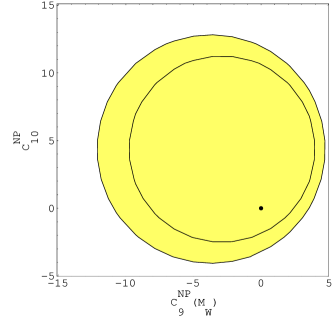
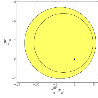
Our analysis is carried out in the effective Hamiltonian approach, obtained by integrating out the heavy degrees of freedom, defined below (see Eq. (1)). However, we make the tacit assumption that the dominant effects of an underlying supersymmetric theory can be implemented by using the SM operator basis for the effective Hamiltonian. Thus, supersymmetric effects enter in our analysis through the modifications of the Wilson coefficients which in the SM are calculated at some high scale, denoted generically by $\mu_{W}$, with the SM anomalous dimension matrix controlling the renormalization of these coefficients to a lower scale, typically $\mu_{b}=O(m_{b})$. Restricting the operator basis to the one in the SM obviously does not cover the most general supersymmetric case, but we think that it covers an important part of the underlying parameter space, and hence can be employed to undertake searches for supersymmetric effects in rare $B$-decays. Within this operator basis, we have split our analysis in two parts. In the first part we update the branching ratios for the decays $B\to(X_{s},K,K^{*})\ell^{+}\ell^{-}$, $\ell=e,\;\mu$, in the standard model. In doing this, we work out the parametric uncertainties due to the scale–dependence, top quark mass, $m_{t}$, and the ratio of the quark masses $m_{c}/m_{b}$. Combining the individual errors $\delta{\cal B}(\mu)$, $\delta{\cal B}(m_{t})$, and $\delta{\cal B}(m_{c}/m_{b})$ in quadrature, we find that the resulting theoretical uncertainties are $\delta{\cal B}(B\to X_{s}e^{+}e^{-})\simeq\pm 15\%$ and $\delta{\cal B}(B\to X_{s}\mu^{+}\mu^{-})\simeq\pm 17\%$. The corresponding theoretical uncertainties on the exclusive decay branching ratios are larger, due to the form factors, and estimated at typically $O(\pm 35\%)$. Using this updated theoretical framework, we extract model-independent constraints that current data (summarized below in Eqs. (4)–(11)) provides on the Wilson coefficients $C_{7}$ – $C_{10}$, which appear in the effective Hamiltonian. We first work out the constraints on $C_{7}$ and $C_{8}$ implied by the $B\to X_{s}\gamma$ measurement. To that end, we define the quantities $R_{7,8}(\mu_{W})\equiv C_{7,8}^{\rm tot}(\mu_{W})/C_{7,8}(\mu_{W})$, and work out bounds on them. Data on $B\to X_{s}\gamma$ allows both $R_{7,8}(\mu_{W})>0$ and $R_{7,8}(\mu_{W})<0$ solutions, which we show in terms of the allowed regions in the $(R_{7}(\mu_{W})$,$R_{8}(\mu_{W}))$ and $(R_{7}(\mu_{b})$,$R_{8}(\mu_{b}))$ planes. We then transcribe the impact of the $B\to(X_{s},K,K^{*})\ell^{+}\ell^{-}$ experimental data on the allowed regions in the $[C_{9},C_{10}]$ plane. Depending on the two branches for the quantities $R_{7,8}(\mu_{W})$, we display the constraints in terms of $C_{9}^{\rm NP}(\mu_{W})$ and $C_{10}^{\rm NP}$. We show that the SM solution (corresponding to the point $(0,0)$ in this plane for the case $R_{7,8}(\mu_{W})=1$) is allowed by present data. More importantly, from the point of view of supersymmetry, our analysis shows the allowed region in the $[C_{9},C_{10}]$ plane, which leaves considerable room for beyond-the-SM contributions to these quantities. In fact, in some allowed regions, phenomenological profiles of semileptonic rare $B$-decays can measurably differ from the corresponding ones in the SM.

The second part of our supersymmetric analysis deals with specific SUSY models and we quantify the additional constraints that the generic $b\to s\ell^{+}\ell^{-}$ data implies for the parameters of these models. We show that no useful bounds beyond what are already known from the $B\to X_{s}\gamma$ analysis are at present obtained in the so–called minimal flavour violating models (including the constrained minimal supersymmetric standard model MSSM) [25]. This reflects the generically small deviations to the SM rates and distributions anticipated in these models, as the allowed supersymmetric parameters are already highly constrained. Working in the mass insertion approximation [26], we show that insertions in the down–squark sector (that enter principally through the gluino penguin and box diagrams) are not constrained either from present data. On the other hand, insertions in the up–squark sector get in some parts of the SUSY parameter space genuinely new constraints. To show possible supersymmetric effects that precise measurements in semileptonic rare $B$-decays may reveal, we work out the forward-backward asymmetry in $B\to X_{s}\ell^{+}\ell^{-}$ for four illustrative points in the $(C_{9}^{\rm NP}(\mu_{W}),C_{10}^{\rm NP})$ plane, representing solutions in the four allowed quadrants in this space. However, a high density scan over all the parameter space shows that the allowed solutions in the models considered by us are scattered mostly around the $(C_{9}^{\rm NP}(\mu_{W}),C_{10}^{\rm NP})=(0,0)$ region, for the two branches for the quantities $R_{7,8}(\mu_{W})$, i.e. for $R_{7,8}(\mu_{W})>0$ and $R_{7,8}(\mu_{W})<0$. We present the resulting constraints on the supersymmetric masses $M_{{\tilde{t}}_{2}}$ (mass of the lighter of the two stop mass eigenstate), $M_{H^{\pm}}$ (the charged Higgs boson masses) and $\tan\beta$ (ratio of the two Higgs vacuum expectation values), in the context of the MFV-MSSM framework, and on the mass insertion parameter $(\delta_{23})$ in the MIA framework. This updates similar results worked out along these lines in Ref. [27].

This paper is organized as follows: In Section 2, we enlist the current measurements of the rare $B$-decays which we have analyzed. The effective Hamiltonian for the SM and the supersymmetric models studied by us is also given here. In Section 3, we present the NNLO implementation of the inclusive and exclusive $b\to s\ell^{+}\ell^{-}$ transitions that we consider. In Section 4 we discuss the branching ratios for the exclusive decays $B\to K^{(*)}\ell^{+}\ell^{-}$ in the SM. In Section 5, we study the constraints on the supersymmetric parameters resulting from the $B\to X_{s}\gamma$ decay in the NLO approximation. In Section 6, we present the results of the model-independent analysis of the $b\to s\ell^{+}\ell^{-}$ modes based on current data. In Section 7, we describe the specific SUSY model that we study and present the bounds on the relevant mass insertions. In Section 8, we summarize our results. Some loop-functions encountered in the calculation and the stop and chargino mass matrices are given in the appendices.

2 Effective Hamiltonian

The effective Hamiltonian in the SM inducing the $b\to s\ell^{+}\ell^{-}$ and $b\to s\gamma$ transitions can be expressed as follows:

$${\cal H}_{\hbox{eff}}=-\frac{4G_{F}}{\sqrt{2}}V_{ts}^{*}V_{tb}\sum_{i=1}^{10}C_{i}(\mu)\,O_{i}(\mu)\quad,$$ (1)

where $O_{i}(\mu)$ are dimension-six operators at the scale $\mu$, $C_{i}(\mu)$ are the corresponding Wilson coefficients, $G_{F}$ is the Fermi coupling constant, and the CKM dependence has been made explicit. The operators can be chosen as Ref. [16]

$$\begin{array}[]{rclrcl}O_{1}&=&(\bar{s}_{L}\gamma_{\mu}T^{a}c_{L})(\bar{c}_{L}\gamma^{\mu}T^{a}b_{L})\,,&O_{2}&=&(\bar{s}_{L}\gamma_{\mu}c_{L})(\bar{c}_{L}\gamma^{\mu}b_{L})\,,\\ \vspace{0.2cm}O_{3}&=&(\bar{s}_{L}\gamma_{\mu}b_{L})\sum_{q}(\bar{q}\gamma^{\mu}q)\,,&O_{4}&=&(\bar{s}_{L}\gamma_{\mu}T^{a}b_{L})\sum_{q}(\bar{q}\gamma^{\mu}T^{a}q)\,,\\ \vspace{0.2cm}O_{5}&=&(\bar{s}_{L}\gamma_{\mu_{1}}\gamma_{\mu_{2}}\gamma_{\mu_{3}}b_{L})\sum_{q}(\bar{q}\gamma^{\mu_{1}}\gamma^{\mu_{2}}\gamma^{\mu_{3}}q)\,,&O_{6}&=&(\bar{s}_{L}\gamma_{\mu_{1}}\gamma_{\mu_{2}}\gamma_{\mu_{3}}T^{a}b_{L})\sum_{q}(\bar{q}\gamma^{\mu_{1}}\gamma^{\mu_{2}}\gamma^{\mu_{3}}T^{a}q)\,,\vspace{0.2cm}\\ \vspace{0.2cm}O_{7}&=&\frac{e}{g_{s}^{2}}m_{b}(\bar{s}_{L}\sigma^{\mu\nu}b_{R})F_{\mu\nu}\,,&O_{8}&=&\frac{1}{g_{s}}m_{b}(\bar{s}_{L}\sigma^{\mu\nu}T^{a}b_{R})G_{\mu\nu}^{a}\,,\\ \vspace{0.2cm}O_{9}&=&\frac{e^{2}}{g_{s}^{2}}(\bar{s}_{L}\gamma_{\mu}b_{L})\sum_{\ell}(\bar{\ell}\gamma^{\mu}\ell)\,,&O_{10}&=&\frac{e^{2}}{g_{s}^{2}}(\bar{s}_{L}\gamma_{\mu}b_{L})\sum_{\ell}(\bar{\ell}\gamma^{\mu}\gamma_{5}\ell)\,,\end{array}$$ (2)

where the subscripts $L$ and $R$ refer to left- and right- handed components of the fermion fields. We work in the approximation where the combination $(V_{us}^{*}V_{ub})$ of the Cabibbo-Kobayashi-Maskawa (CKM) matrix elements [28] is neglected; in this case the CKM structure factorizes, as indicated in Eq. (1). Of course, for the sake of book keeping, one can keep the individual top-quark and charm-quark contributions in the loop separately, but as there is no way to distinguish these individual contributions we will give the results in the summed form.

Note the inverse powers of $g_{s}$ in the definition of the operators $O_{7}$,…,$O_{10}$ in Eq. (2). These factors have been introduced by Misiak in Ref. [29] in order to simplify the organization of the calculations. In this framework, the LO result for the $b\to s\ell^{+}\ell^{-}$ decay amplitude is obtained in the following three steps: the matching conditions $C_{i}(\mu_{W})$ have to be worked out at $O(\alpha_{s}^{0})$, the renormalization group evolution has to be performed using the $O(\alpha_{s}^{1})$ anomalous dimension matrix and the matrix elements of the operators $O_{i}$ have to be worked out at order $1/\alpha_{s}$. In going to the NLO precision all the three steps have to be improved by one order in $\alpha_{s}$.

At an arbitrary scale $\mu$ the Wilson coefficients can be decomposed as

$$C_{i}(\mu)=C_{i}^{(0)}(\mu)+\frac{\alpha_{s}(\mu)}{4\pi}\,C_{i}^{(1)}(\mu)+\frac{\alpha^{2}_{s}(\mu)}{(4\pi)^{2}}\,C_{i}^{(2)}(\mu)+\ldots\quad.$$ (3)

We note that in our basis only $C_{2}$ is different from zero at the matching scale $\mu_{W}$ at leading order, viz. $C_{i}^{(0)}(\mu_{W})=\delta_{i2}$. At the low scale $\mu_{b}$ (of order $m_{b}$), the coefficients $C_{i}^{0}(\mu_{b})$ are non-zero for $i=1,...,6;9$ whereas they vanish for $i=7,8,10$.

We shall use this effective Hamiltonian and calculate the matrix elements for the decays of interest, specifying the degree of theoretical accuracy.

The experimental input that we use in our analysis is given below. Except for the inclusive branching ratio for $B\to X_{s}\gamma$, which is the average of the results from CLEO, ALEPH and BELLE measurements [3, 4, 5], all other entries are taken from the two BELLE papers listed in Ref. [10]:

$${\cal B}(B\to X_{s}\gamma) = (3.22\pm 0.40)\times 10^{-4}\;,$$ (4)

$${\cal B}(B\to K\mu^{+}\mu^{-}) = (0.99^{+0.40+0.13}_{-0.32-0.14})\times 10^{-6}\;,$$ (5)

$${\cal B}(B\to Ke^{+}e^{-}) = (0.48^{+0.32+0.09}_{-0.24-0.11})\times 10^{-6}\;,$$ (6)

$${\cal B}(B\to K\ell^{+}\ell^{-}) = (0.75^{+0.25}_{-0.21}\pm 0.09)\times 10^{-6}\;,$$ (7)

$${\cal B}(B\to K^{*}\mu^{+}\mu^{-}) \leq 3.0\times 10^{-6}\;{\rm at}\;{90\%\ \mathrm{C.L.}}\;,$$ (8)

$${\cal B}(B\to K^{*}e^{+}e^{-}) \leq 5.1\times 10^{-6}\;{\rm at}\;{90\%\ \mathrm{C.L.}}\;,$$ (9)

$${\cal B}(B\to X_{s}\mu^{+}\mu^{-}) \leq 19.1\times 10^{-6}\;{\rm at}\;{90\%\ \mathrm{C.L.}}\;,$$ (10)

$${\cal B}(B\to X_{s}e^{+}e^{-}) \leq 10.1\times 10^{-6}\;{\rm at}\;{90\%\ \mathrm{C.L.}}\;.$$ (11)

The experimental numbers given in Eqs. (5) – (11) refer to the so–called non–resonant branching ratios integrated over the entire dilepton invariant mass spectrum. In the experimental analyses, judicious cuts are used to remove the dominant resonant contributions arising from the decays $B\to(X_{s},K,K^{*})(J/\psi,\psi^{\prime},...)\to(X_{s},K,K^{*})\ell^{+}\ell^{-}$. A direct comparison of experiment and theory is, of course, very desirable, but we do not have access to this restricted experimental information. Instead, we compare the theoretical predictions with data which has been corrected for the experimental acceptance using SM-based theoretical distributions from Ref. [14, 15]. In the present analysis, we are assuming that the acceptance corrections have been adequately incorporated in the experimental analysis in providing the branching ratios and upper limits listed above. We will give the theoretical branching ratios integrated over all dilepton invariant masses to compare with these numbers. However, for future analyses, we emphasize the dilepton invariant mass distribution in the low-$\hat{s}$ region, $\hat{s}\equiv m_{\ell^{+}\ell^{-}}^{2}/m_{b,pole}^{2}\leq 0.25$, where the NNLO calculations for the inclusive decays are known, and resonant effects due to $J/\psi$, $\psi^{\prime}$, etc. are expected to be small.

3 Inclusive $b\to s\ell^{+}\ell^{-}$ decays at NNLO

We start by discussing the NNLO analysis of the $B\to X_{s}\ell^{+}\ell^{-}$ decays presented in Refs. [16, 17], recalling that the $O(\alpha_{s})$ corrections to the matrix elements computed in Ref. [17] have been calculated only below the $c\bar{c}$ resonances.

In the NNLO approximation, the invariant dilepton mass distribution for the inclusive decay $B\to X_{s}\ell^{+}\ell^{-}$ can be written as

$$\frac{d\Gamma(b\to X_{s}\ell^{+}\ell^{-})}{d\hat{s}}=\left(\frac{\alpha_{em}}{4\pi}\right)^{2}\frac{G_{F}^{2}m_{b,pole}^{5}\left|V_{ts}^{*}V_{tb}\right|^{2}}{48\pi^{3}}(1-\hat{s})^{2}\times$$

$$\left(\left(1+2\hat{s}\right)\left(\left|\widetilde{C}_{9}^{\hbox{eff}}\right|^{2}+\left|\widetilde{C}_{10}^{\hbox{eff}}\right|^{2}\right)+4\left(1+2/\hat{s}\right)\left|\widetilde{C}_{7}^{\hbox{eff}}\right|^{2}+12\mbox{Re}\left(\widetilde{C}_{7}^{\hbox{eff}}\widetilde{C}_{9}^{\hbox{eff}*}\right)\right)\,.$$ (12)

In the SM the effective Wilson coefficients $\tilde{C}_{7}^{\hbox{eff}}$, $\tilde{C}_{9}^{\hbox{eff}}$ and $\tilde{C}_{10}^{\hbox{eff}}$ are given by [16, 17]

$$\widetilde{C}_{7}^{\hbox{eff}} = \left(1+\frac{\alpha_{s}(\mu)}{\pi}\omega_{7}(\hat{s})\right)\,A_{7}$$ (13)

$$-\frac{\alpha_{s}(\mu)}{4\pi}\left(C_{1}^{(0)}F_{1}^{(7)}(\hat{s})+C_{2}^{(0)}F_{2}^{(7)}(\hat{s})+A_{8}^{(0)}F_{8}^{(7)}(\hat{s})\right)\,,$$

$$\widetilde{C}_{9}^{\hbox{eff}} = \left(1+\frac{\alpha_{s}(\mu)}{\pi}\omega_{9}(\hat{s})\right)\left(A_{9}+T_{9}\,h(\hat{m}_{c}^{2},\hat{s})+U_{9}\,h(1,\hat{s})+W_{9}\,h(0,\hat{s})\right)$$ (14)

$$-\frac{\alpha_{s}(\mu)}{4\pi}\left(C_{1}^{(0)}F_{1}^{(9)}(\hat{s})+C_{2}^{(0)}F_{2}^{(9)}(\hat{s})+A_{8}^{(0)}F_{8}^{(9)}(\hat{s})\right)\,,$$

$$\widetilde{C}_{10}^{\hbox{eff}} = \left(1+\frac{\alpha_{s}(\mu)}{\pi}\omega_{9}(\hat{s})\right)\,A_{10}\,,$$ (15)

where the functions $h(\hat{m}_{c}^{2},\hat{s})$ and $\omega_{9}(\hat{s})$ are given in Ref. [16], while $\omega_{7}(\hat{s})$ and $F_{1,2,8}^{(7,9)}(\hat{s})$ can be seen in Ref. [17]. The auxiliary quantities $A_{7}$, $A_{8}$, $A_{9}$, $A_{10}$, $T_{9}$, $U_{9}$, $W_{9}$ are the following linear combinations of the Wilson coefficients $C_{i}(\mu)$ (see Eq.(1)):

$$A_{7} = \frac{4\pi}{\alpha_{s}(\mu)}\,C_{7}(\mu)-\frac{1}{3}\,C_{3}(\mu)-\frac{4}{9}\,C_{4}(\mu)-\frac{20}{3}\,C_{5}(\mu)-\frac{80}{9}\,C_{6}(\mu)\,,$$ (16)

$$A_{8} = \frac{4\pi}{\alpha_{s}(\mu)}\,C_{8}(\mu)+C_{3}(\mu)-\frac{1}{6}\,C_{4}(\mu)+20\,C_{5}(\mu)-\frac{10}{3}\,C_{6}(\mu)\,,$$ (17)

$$A_{9} = \frac{4\pi}{\alpha_{s}(\mu)}\,C_{9}(\mu)+\sum_{i=1}^{6}\,C_{i}(\mu)\,\gamma_{i9}^{(0)}\,\ln\frac{m_{b}}{\mu}$$ (18)

$$+\frac{4}{3}\,C_{3}(\mu)+\frac{64}{9}\,C_{5}(\mu)+\frac{64}{27}\,C_{6}(\mu)\,,$$

$$A_{10} = \frac{4\pi}{\alpha_{s}(\mu)}\,C_{10}(\mu)\,,$$ (19)

$$T_{9} = +\frac{4}{3}\,C_{1}(\mu)+C_{2}(\mu)+6\,C_{3}(\mu)+60\,C_{5}(\mu)\,,$$ (20)

$$U_{9} = -\frac{7}{2}\,C_{3}(\mu)-\frac{2}{3}\,C_{4}(\mu)-38\,C_{5}(\mu)-\frac{32}{3}\,C_{6}(\mu)\,,$$ (21)

$$W_{9} = -\frac{1}{2}\,C_{3}(\mu)-\frac{2}{3}\,C_{4}(\mu)-8\,C_{5}(\mu)-\frac{32}{3}\,C_{6}(\mu)\,.$$ (22)

The elements $\gamma_{i9}^{(0)}$ can be seen in Eq. (26) of ref. [16]. $A_{8}^{(0)}$ in Eqs. (13) and (14) denotes the lowest order piece of $A_{8}$:

$$A_{8}^{(0)}=C_{8}^{(1)}(\mu)+C_{3}^{(0)}(\mu)-\frac{1}{6}\,C_{4}^{(0)}(\mu)+20\,C_{5}^{(0)}(\mu)-\frac{10}{3}\,C_{6}^{(0)}(\mu)\,.$$ (23)

The numerical values for the coefficients $A_{7}$, $A_{8}^{(0)}$, $A_{9}$, $A_{10}$, $T_{9}$, $U_{9}$, $W_{9}$, $C_{1}$ and $C_{2}$ are obtained after solving the renormalization group equations for the Wilson coefficients $C_{i}(\mu)$, using the matching conditions from ref. [16] and the anomalous dimension matrices from Refs. [16, 6]. As mentioned earlier, we do not separate charm- and top- quark contributions and perform the matching (for both) at the scale $\mu_{W}=m_{W}$. The resulting values are summarized in Table 1. Note that when calculating the decay width (3), we retain only terms linear in $\alpha_{s}$ (and thus in $\omega_{9}$ and $\omega_{7}$) in $|\widetilde{C}_{9}^{\hbox{eff}}|^{2}$ and $|\widetilde{C}_{7}^{\hbox{eff}}|^{2}$. In the interference term $\mbox{Re}\left(\widetilde{C}_{7}^{\hbox{eff}}\widetilde{C}_{9}^{\hbox{eff}*}\right)$ too, we keep only terms linear in $\alpha_{s}$. By construction, one has to make the replacements $\omega_{9}\to\omega_{79}$ and $\omega_{7}\to\omega_{79}$ in this term where the function $\omega_{79}(\hat{s})$ can be found in Ref. [17].

We now turn to the modifications of the effective Wilson coefficients $\widetilde{C}_{7}^{\hbox{eff}}$, $\widetilde{C}_{9}^{\hbox{eff}}$ and $\widetilde{C}_{10}^{\hbox{eff}}$ in the presence of new physics which enters through a modification of the Wilson coefficients $C_{7}$, $C_{8}$, $C_{9}$ and $C_{10}$ at the matching scale $\mu_{W}$. By doing so, we tacitly assume that the scale of new physics is close enough to the weak scale $m_{W}$, justifying to integrate out simultaneously the heavy SM particles and the additional ones present in the new physics scenario. For simplicity we assume that only the lowest non-trivial order of these Wilson coefficients get modified by new physics, which in our setup (see Eqs. (1),(2),(3)) means that $C_{7}^{(1)}(\mu_{W})$, $C_{8}^{(1)}(\mu_{W})$, $C_{9}^{(1)}(\mu_{W})$, $C_{10}^{(1)}(\mu_{W})$ get modified. The shifts of the Wilson coefficients at $\mu_{W}$ can be written as:

$$C_{i}(\mu_{W})\longrightarrow C_{i}(\mu_{W})+\frac{\alpha_{s}}{4\pi}\,C_{i}^{NP}(\mu_{W})\,.$$ (24)

These shift at the matching scale are translated through the RGE step into modifications of the coefficients $C_{i}(\mu_{b})$ at the low scale $\mu_{b}$, leading in turn to modifications of the effective Wilson coefficients defined in Eqs. (13–15). They now read

$$\widetilde{C}_{7}^{\hbox{eff}} = \left(1+\frac{\alpha_{s}(\mu)}{\pi}\omega_{7}(\hat{s})\right)(A_{7}+A_{77}\;C_{7}^{NP}(\mu_{W})+A_{78}\;C_{8}^{NP}(\mu_{W}))$$ (25)

$$-\frac{\alpha_{s}(\mu)}{4\pi}\left(C_{1}^{(0)}F_{1}^{(7)}(\hat{s})+C_{2}^{(0)}F_{2}^{(7)}(\hat{s})+A_{8}^{(0)}F_{8}^{(7)}(\hat{s})+A_{88}^{(0)}\,C_{8}^{NP}(\mu_{W})\,F_{8}^{(7)}(\hat{s})\right)\,,$$

$$\widetilde{C}_{9}^{\hbox{eff}} = \left(1+\frac{\alpha_{s}(\mu)}{\pi}\omega_{9}(\hat{s})\right)\left(A_{9}+T_{9}\,h(\hat{m}_{c}^{2},\hat{s})+U_{9}\,h(1,\hat{s})+W_{9}\,h(0,\hat{s})+C_{9}^{NP}(\mu_{W})\right)$$ (26)

$$-\frac{\alpha_{s}(\mu)}{4\pi}\left(C_{1}^{(0)}F_{1}^{(9)}(\hat{s})+C_{2}^{(0)}F_{2}^{(9)}(\hat{s})+A_{8}^{(0)}F_{8}^{(9)}(\hat{s})+A_{88}^{(0)}\,C_{8}^{NP}(\mu_{W})\,F_{8}^{(9)}(\hat{s})\right)\,,$$

$$\widetilde{C}_{10}^{\hbox{eff}} = \left(1+\frac{\alpha_{s}(\mu)}{\pi}\omega_{9}(\hat{s})\right)(A_{10}+C_{10}^{NP})\,.$$ (27)

The numerical values for the parameters $A_{77}$, $A_{78}$, $A_{88}^{(0)}$, which incorporate the effects from the running, are listed in Table 1.

	$\mu=2.5$ GeV	$\mu=5$ GeV	$\mu=10$ GeV
$\alpha_{s}$	$0.267$	$0.215$	$0.180$
$(C_{1}^{(0)},C_{1}^{(1)})$	$(-0.697,0.241)$	$(-0.487,0.207)$	$(-0.326,0.184)$
$(C_{2}^{(0)},C_{2}^{(1)})$	$(1.046,-0.028)$	$(1.024,-0.017)$	$(1.011,-0.010)$
$(A_{7}^{(0)},A_{7}^{(1)})$	$(-0.353,0.023)$	$(-0.312,0.008)$	$(-0.278,-0.002)$
$(A_{77}^{(0)},A_{77}^{(1)})$	$(0.577,-0.0524)$	$(0.672,-0.0391)$	$(0.760,-0.0277)$
$(A_{78}^{(0)},A_{78}^{(1)})$	$(0.109,-0.00520)$	$(0.0914,-0.00193)$	$(0.0707,-0.000263)$
$A_{8}^{(0)}$	$-0.164$	$-0.148$	$-0.134$
$A_{88}^{(0)}$	$0.618$	$0.706$	$0.786$
$(A_{9}^{(0)},A_{9}^{(1)})$	$(4.287,-0.218)$	$(4.174,-0.035)$	$(4.177,0.107)$
$(T_{9}^{(0)},T_{9}^{(1)})$	$(0.114,0.280)$	$(0.374,0.252)$	$(0.575,0.231)$
$(U_{9}^{(0)},U_{9}^{(1)})$	$(0.045,0.023)$	$(0.033,0.015)$	$(0.022,0.010)$
$(W_{9}^{(0)},W_{9}^{(1)})$	$(0.044,0.016)$	$(0.032,0.012)$	$(0.022,0.008)$
$(A_{10}^{(0)},A_{10}^{(1)})$	$(-4.592,0.379)$	$(-4.592,0.379)$	$(-4.592,0.379)$

Table 1: Coefficients appearing in Eqs. (13–15) and Eqs. (25–27) for three different scales $\mu=2.5$ GeV, $\mu=5$ GeV and $\mu=10$ GeV. For $\alpha_{s}(\mu)$ (in the $\overline{\mbox{MS}}$ scheme) we used the two-loop expression with 5 flavours and $\alpha_{s}(m_{Z})=0.119$. The entries correspond to the $\overline{MS}$ top quark mass renormalized at the scale $m_{W}$, $m_{t}(m_{W})=175.9\;{\hbox{GeV}}$. The superscript $(0)$ refers to the lowest order quantities while the superscript $(1)$ denotes the correction terms of order $\alpha_{s}$, i.e. $X=X^{(0)}+X^{(1)}$ with $X=C,A,T,U,W$.

3.1 Power corrections in inclusive $B\to X_{s}\ell^{+}\ell^{-}$ decays

Before presenting a theoretical analysis of the available data on rare $B$-decays, we would like to discuss power corrections in the inclusive $B\to X_{s}\ell^{+}\ell^{-}$ decays. In the NNLO approximation and including leading order power corrections in $1/m_{b}$ [14] and $1/m_{c}$ [19], the invariant dilepton mass distribution for the inclusive decay $B\to X_{s}\ell^{+}\ell^{-}$ can be written as

$$\frac{d\Gamma(b\to s\ell^{+}\ell^{-})}{d\hat{s}} = \left(\frac{\alpha_{em}}{4\pi}\right)^{2}\frac{G_{F}^{2}m_{b,pole}^{5}\left|V_{ts}^{*}V_{tb}\right|^{2}}{48\pi^{3}}(1-\hat{s})^{2}\left[\left(1+2\hat{s}\right)\left(\left|\widetilde{C}_{9}^{\hbox{eff}}\right|^{2}+\left|\widetilde{C}_{10}^{\hbox{eff}}\right|^{2}\right)G_{1}(\hat{s})\right.$$ (28)

$$+ \left.4\left(1+2/\hat{s}\right)\left|\widetilde{C}_{7}^{\hbox{eff}}\right|^{2}G_{2}(\hat{s})+12\mbox{Re}\left(\widetilde{C}_{7}^{\hbox{eff}}\widetilde{C}_{9}^{\hbox{eff}*}\right)G_{3}(\hat{s})+G_{c}(\hat{s})\right]\,.$$

where

$$G_{1}(\hat{s}) = 1+\frac{\lambda_{1}}{2m_{b}^{2}}+3\frac{1-15\hat{s}^{2}+10\hat{s}^{3}}{(1-\hat{s})^{2}(1+2\hat{s})}\frac{\lambda_{2}}{2m_{b}^{2}}$$ (29)

$$G_{2}(\hat{s}) = 1+\frac{\lambda_{1}}{2m_{b}^{2}}-3\frac{6+3\hat{s}-5\hat{s}^{3}}{(1-\hat{s})^{2}(2+\hat{s})}\frac{\lambda_{2}}{2m_{b}^{2}}~{},$$ (30)

$$G_{3}(\hat{s}) = 1+\frac{\lambda_{1}}{2m_{b}^{2}}-\frac{5+6\hat{s}-7\hat{s}^{2}}{(1-\hat{s})^{2}}\frac{\lambda_{2}}{2m_{b}^{2}}~{}.$$ (31)

The values of the heavy quark matrix elements $\lambda_{1}$ and $\lambda_{2}$ that we use in our analysis are given in Table 2. The term denoted by $G_{c}$ takes $1/m_{c}$ corrections into account. It is written as

$$G_{c}(\hat{s})=-\frac{8}{9}(C_{2}-\frac{C_{1}}{6})\frac{\lambda_{2}}{m_{c}^{2}}\mbox{Re}\left(F^{*}(r)\left[\widetilde{C}_{9}^{\hbox{eff}}(2+\hat{s})+\widetilde{C}_{7}^{\hbox{eff}}\frac{1+6\hat{s}-\hat{s}^{2}}{\hat{s}}\right]\right)~{}.$$ (32)

Since our basis in Eq. (2) is different from the one often used in the literature i.e. $\tilde{O}_{1}=(\bar{s}_{L}\gamma_{\mu}b_{L})(\bar{c}_{L}\gamma^{\mu}c_{L})$ and $O_{1}=\tilde{O}_{1}/2-O_{2}/6$, Eq. (32) differs superficially from the one reported in [19]. The function $F(r)$, where $r=\hat{s}/(4\hat{m}_{c}^{2})$, is given below [19]:

$$F(r)=\frac{3}{2r}\left\{\begin{array}[]{ll}\displaystyle\frac{1}{\sqrt{r(1-r)}}\arctan\sqrt{\frac{r}{1-r}}-1&\qquad\qquad 0<r<1~{},\\ \displaystyle\frac{1}{2\sqrt{r(r-1)}}\left(\ln\frac{1-\sqrt{1-1/r}}{1+\sqrt{1-1/r}}+i\pi\right)-1&\qquad\qquad r>1~{}.\end{array}\right.$$ (33)

The impact of power corrections in inclusive decays $B\to X_{s}\ell^{+}\ell^{-}$ at NLO has been studied in [18] in the SM. In the low dilepton mass region and for $q^{2}$ not too close to the photon pole where $O_{7}$ dominates, the $1/m_{b}$ effects enhance the rate by $\sim 1\%$. In the high–$\hat{s}$ region they become negative and decrease the rate by few percent. Their magnitude rises more and more towards the boundary $q^{2}\sim m_{b}^{2}$, where the expansion in $1/m_{b}$ breaks down [14]. The $1/m_{c}$ expansion Eq. (32) is valid everywhere except near threshold $\hat{s}=4\hat{m}_{c}^{2}$, and it also fails at the charmonium resonances $J/\Psi$ and higher ones like $\Psi^{\prime}$. The $1/m_{c}$ corrections decrease the rate below the charm threshold and enhance it above by few percent.

This is illustrated in Figure 1, where the relative size $R(\hat{s})$ of the combined $1/m_{b}$ and $1/m_{c}$ corrections defined as

$$R(\hat{s})\equiv\frac{\frac{d\Gamma(b\to X_{s}\ell^{+}\ell^{-})}{d\hat{s}}{\rm(with\;power\,corrections)}-\frac{d\Gamma(b\to X_{s}\ell^{+}\ell^{-})}{d\hat{s}}{\rm(no\;power\,corrections)}}{\frac{d\Gamma(b\to X_{s}\ell^{+}\ell^{-})}{d\hat{s}}{\rm(with\;power\,corrections)}}$$ (34)

is shown for the SM, and for comparison also for $C_{7}=-C_{7}^{SM}$. Both $1/m$ correction thus partially cancel in the SM. The situation with new physics can be different. In a generic scenario with $C_{7}=-C_{7}^{SM}$ the power corrections can be more pronounced, in particular for low dilepton mass where both $1/m$ corrections are negative. Together they lower the rate by few percent. Note that in our estimates of the $B\to X_{s}\ell^{+}\ell^{-}$ branching ratio, we include the power corrections in the semileptonic branching ratios [30] as well.

3.2 Branching ratios for $B\to X_{s}\ell^{+}\ell^{-}$ in the SM

In order to eliminate the large uncertainty due to the factor $m_{b,pole}^{5}$ appearing in the decay width for $B\to X_{s}\ell^{+}\ell^{-}$, it has become customary to consider instead the following branching ratio

$${\cal B}^{B\to X_{s}\ell^{+}\ell^{-}}(\hat{s})={{\cal B}_{\hbox{\tiny exp}}^{B\to X_{c}e\bar{\nu}}\over\Gamma(B\to X_{c}e\bar{\nu})}{d\Gamma(B\to X_{s}\ell^{+}\ell^{-})\over d\hat{s}}\,,$$ (35)

in which the factor $m_{b,pole}^{5}$ drops out. The explicit expression for the semi-leptonic decay width $\Gamma(B\to X_{c}e\nu_{e})$ can be found e.g. in Ref. [16]. Note that as we are ignoring the annihilation contributions, which lead to isospin violations in the decay widths, and we are using the averaged semileptonic branching ratio to normalize, all our inclusive branching ratios are to be understood as averaged over the $B^{\pm}$ and $B^{0}(\overline{B^{0}})$ decays.

The dilepton invariant mass distribution for the process $B\to X_{s}e^{+}e^{-}$ calculated in NNLO is shown in Fig. 2 for the three choices of the scale $\mu=2.5~{}{\hbox{GeV}}$, $\mu=5~{}{\hbox{GeV}}$ and $\mu=~{}10~{}{\hbox{GeV}}$ (solid curves). In this figure, the left-hand plot shows the distribution in the very low invariant mass region ($\hat{s}\in[0,0.05]$, with $0$ to be understood as the kinematic threshold $s=4m_{e}^{2}\simeq 10^{-6}\;{\hbox{GeV}}^{2}$, yielding $\hat{s}=4.5\times 10^{-8}$), and the right-hand plot shows the dilepton spectrum in the region beyond $\hat{s}>0.05$, and hence this also holds for the decay $B\to X_{s}\mu^{+}\mu^{-}$. We should stress at this point that a genuine NNLO calculation only exists for values of $\hat{s}$ below 0.25, which is indicated in the right-hand plot by the vertical dotted line. For higher values of $\hat{s}$, an estimate of the NNLO result is obtained by an extrapolation procedure discussed in more detail at the end of this paragraph. The so-called partial NNLO dilepton spectrum, obtained by switching off the quantities $F_{1,2,8}^{(7,9)}$ in Eqs. (13) and (14), is also shown in each of these cases for the same three choices of the scale $\mu$ (dashed curves). Note that in the left-hand plot, the lowest lying curves are for $\mu=10~{}{\hbox{GeV}}$ and the uppermost ones are for $\mu=2.5\;{\hbox{GeV}}$. In the right-hand plot, the scale-dependence is reversed, i.e., the highest lying curves are for $\mu=~{}10~{}{\hbox{GeV}}$ and the lowest for $\mu=2.5~{}{\hbox{GeV}}$. The crossing (in the partial NNLO BR) happens near $\hat{s}=0.04$ and this feature leads to a certain cancellation of the $\mu$ dependence in the decay rate for $B\to X_{s}e^{+}e^{-}$. We also note that the NNLO dilepton invariant mass spectrum in the right-hand plot ($\hat{s}>0.05$) lies below its partial NNLO counterpart, and hence the partial branching ratios for both the $B\to X_{s}e^{+}e^{-}$ and $B\to X_{s}\mu^{+}\mu^{-}$ decays are reduced in the full NNLO accuracy. More importantly, from the point of view of our subsequent analysis, Fig. 2 shows that the full NNLO invariant mass distribution is very well approximated by the partial NNLO for the choice of the scale $\mu=2.5\;{\hbox{GeV}}$, in the entire low-$\hat{s}$ range. This is yet another illustration of the situation often met in perturbation theory that a judicious choice of the scale reduces the higher order corrections. From this observation, it seems reasonable to use the partial NNLO curve corresponding to $\mu_{b}=2.5\;{\hbox{GeV}}$ as an estimate for the central value of the full NNLO for $\hat{s}>0.25$. We estimate the scale dependence in this region by assuming that it is given by the genuine NNLO calculation at $\hat{s}=0.25$.

In order to complete our discussion of the computation of the inclusive branching ratios, it is necessary to discuss their dependence on the quark masses $m_{t}$ and $m_{c}$ (in particular, the latter is marked for what concerns the SM prediction). We vary both masses within the errors that we quote in Table 2 and present the results for the branching ratios $B\to X_{s}e^{+}e^{-}$ and $B\to X_{s}\mu^{+}\mu^{-}$ in Table 3 where we include also the power corrections discussed in Sec. 3.1. In Table 4 we show the SM central values and the parametric uncertainties by means of independent error bars (to be interpreted as ${68\%\ \mathrm{C.L.}}$ uncertainties). In this table, the first error on the exclusive channel is due to the form factors, and is by far the dominant one. The other errors in both the exclusive and inclusive decays come from the scale ($\mu_{b}$), $m_{t,pole}$ and $m_{c}/m_{b}$ respectively. Summing the errors in quadrature we get for the inclusive decays:

$${\cal B}(B\to X_{s}e^{+}e^{-}) = (6.89\pm 1.01)\times 10^{-6}\;\;\;(\delta{\cal B}_{X_{s}ee}=\pm 15\%)\;,$$ (36)

$${\cal B}(B\to X_{s}\mu^{+}\mu^{-}) = (4.15\pm 0.70)\times 10^{-6}\;\;\;(\delta{\cal B}_{X_{s}\mu\mu}=\pm 17\%)\;.$$ (37)

Using the same input parameters, but restricting to the NLO precision, the inclusive branching ratios have the central values ${\cal B}(B\to X_{s}e^{+}e^{-})=7.8\times 10^{-6}$ and ${\cal B}(B\to X_{s}\mu^{+}\mu^{-})=5.2\times 10^{-6}$. Thus, NNLO corrections reduce the branching ratios by typically $12\%$ and $20\%$, respectively. In Ref. [8], it was recently suggested in the context of the decay $B\to X_{s}\gamma$, where the charm quark mass enters the matrix elements at the two-loop level only, that it would be more appropriate to use the running charm mass evaluated at the $\mu_{b}\simeq O(m_{b})$ scale, leading to $m_{c}/m_{b}\simeq 0.22$. Intuitively, this is a reasonable choice since the charm quark enters only as virtual particle running inside loops; formally, on the other hand, it is also clear that the difference between the results obtained by interpreting $m_{c}$ as the pole mass or the running mass is a higher order QCD effect. In what concerns $B\to X_{s}\ell^{+}\ell^{-}$, the situation is somewhat different, as the charm quark mass enters in this case also in the one-loop matrix elements associated with $O_{1}$ and $O_{2}$. In these one-loop contributions, $m_{c}$ has the meaning of the pole mass when using the expressions derived in Ref. [17]. Concerning the charm quark mass in the two-loop expressions, the definition $m_{c}$ is not fixed, like in $B\to X_{s}\gamma$. In our analysis, we prefer not to include this effect related to the definition of the charm quark mass in the final errors that we have listed.

4 Exclusive $B\to K^{(*)}\ell^{+}\ell^{-}$ decays

For what concerns the exclusive decays $B\to K^{(*)}\ell^{+}\ell^{-}$, we implement the NNLO corrections calculated by Bobeth et al. in Ref. [16] and by Asatrian et al. in Ref. [17] for the short-distance contribution. Then, we use the form factors calculated with the help of the QCD sum rules in Ref. [15]. Note that, in this case, we have dropped the contribution to the matrix elements given by the functions $\omega_{i}(\hat{s})$ since this can be regarded as included in the full QCD form factors. In adopting this procedure, we are ignoring the so-called hard spectator corrections, calculated in the decays $B\to K^{*}\ell^{+}\ell^{-}$ [21] in the large energy limit of QCD [31], necessarily limiting the invariant mass to the small-$s$ region. The findings of Ref. [21] are that the dilepton invariant mass distribution in this region is rather stable against the explicit $O(\alpha_{s})$ corrections, and the theoretical uncertainties are dominated by the form factors and other non-perturbative parameters specific to the large-energy factorization approach. This is so, even if one takes the point of view that the form factor $\xi_{\perp}(0)$, governing the transition $B\to K^{*}$ to the transversely polarized $K^{*}$-meson, can be assumed known from the analysis of the radiative transition $B\to K^{*}\gamma$ in this approach and current data, as it is the contribution of the longitudinally polarized $K^{*}$ which dominates the decay rate in the small-$\hat{s}$ range, for which a knowledge of $\xi_{\parallel}$ is required. In principle, using estimates of SU(3)-breaking and HQET, the function $\xi_{\parallel}$ for the decays $B\to K^{*}\ell^{+}\ell^{-}$ can be obtained from the semileptonic decays $B\to\rho\ell\nu_{\ell}$. However, as present data on the $Q^{2}$-dependence in the decay $B\to\rho\ell\nu_{\ell}$ is rather sparse and a helicity-based analysis of the decays $B\to\rho\ell\nu_{\ell}$ has yet to be undertaken, one will have to resort to form factor models for $\xi_{\parallel}$, which as opposed to the transverse form factor $\xi_{\perp}$, is essentially unbounded. In view of this, we ignore the hard spectator correction and discuss a plausible range of the form factors in the decays $B\to(K,K^{*})\ell^{+}\ell^{-}$.

As already stated, some inference about the magnetic moment form factor $T_{1}(0)$, involving the matrix element of the operator $O_{7}$ in the decay $B\to K^{*}\gamma$, has been derived by comparing the explicit $O(\alpha_{s})$ and $\Lambda_{\rm QCD}/M_{B}$ corrected branching ratios in the factorization approach with data [20, 21, 22]. One finds that present data on $B\to K^{*}\gamma$ decay yields typically a value in the range $T_{1}(0)=0.28\pm 0.04$. This suggests that, including the explicit $O(\alpha_{s})$ corrections, data requires a value of this form factor which is smaller than its typical QCD sum rule estimate. To accommodate this, we use the minimum allowed form factors obtained in the light-cone QCD sum rule formalism, given in Table 5 of Ref. [15], as our default set. This, for example, corresponds to setting $T_{1}(0)=0.33$. In our numerical analysis, we add a flat $\pm 15\%$ error as residual uncertainty on the form factors. Thus, the input range for $T_{1}(0)$ in our analysis $T_{1}(0)=0.33\pm 0.05$ overlaps with the phenomenologically extracted value in the factorization approach given earlier. Again, following the argument given earlier for the inclusive decays, we set $\mu_{b}=2.5\;{\hbox{GeV}}$, and include the NNLO corrections in an analogous fashion to the inclusive $B\to X_{s}\ell^{+}\ell^{-}$ case. The explicit expressions for the $B\to K^{(*)}\ell^{+}\ell^{-}$ branching ratios can be found, for example, in Ref. [15].

The input parameters that we use in the analyses are summarized in Table 2. Our SM predictions for the above discussed inclusive and exclusive branching ratios are summarized in Table 4. Note that the dominant source of uncertainty comes from the form factors dependence. Summing the errors in quadrature we obtain:

$${\cal B}(B\to K\ell^{+}\ell^{-}) = (0.35\pm 0.12)\times 10^{-6}\;\;\;(\delta{\cal B}_{K\ell\ell}=\pm 34\%)\;,$$ (38)

$${\cal B}(B\to K^{*}e^{+}e^{-}) = (1.58\pm 0.49)\times 10^{-6}\;\;\;(\delta{\cal B}_{K^{*}ee}=\pm 31\%)\;,$$ (39)

$${\cal B}(B\to K^{*}\mu^{+}\mu^{-}) = (1.19\pm 0.39)\times 10^{-6}\;\;\;(\delta{\cal B}_{K^{*}\mu\mu}=\pm 33\%)\;.$$ (40)

Note that the dependence of the exclusive decay branching ratios on $m_{c}/m_{b}$ is much milder, as we are using the ($m_{c}/m_{b}$-independent) lifetime $\tau(B^{0})$ in calculating the branching ratios for exclusive decays, as opposed to the inclusive decays $B\to X_{s}\ell^{+}\ell^{-}$, where the semileptonic branching ratios are used for normalization. Since the semileptonic decay widths depend on $m_{c}/m_{b}$, this sensitivity goes over to the inclusive decay branching ratios for $B\to X_{s}\ell^{+}\ell^{-}$. Note also that as we have used $\tau(B^{0})$ in calculating the branching ratios for exclusive decays, all the branching ratios given above are for the $B^{0}(\overline{B^{0}})$ decays. The ones for the $B^{\pm}$-decays can be scaled by taking into account the lifetime difference.

$m_{Z}$	$91.1867\;{\hbox{GeV}}$	$\alpha_{s}(m_{Z})$	0.119 [
$m_{W}$	$80.41\;{\hbox{GeV}}$	$\alpha_{e}$	1/133 [
$m_{b,pole}$	$4.8\;{\hbox{GeV}}$	$\sin^{2}\theta_{W}$	0.23124 [
$m_{t,pole}$	$(173.8\pm 5)\;{\hbox{GeV}}$	$G_{F}$	$1.16639\times 10^{-5}\;{\hbox{GeV}}^{-2}$ [
$\tau_{B^{0}}$	$1.54\;{\rm ps}$	$|V_{tb}V_{ts}^{*}|$	0.038 [
${\cal B}_{\hbox{\tiny exp}}^{B\to X_{c}e\bar{\nu}}$	$0.104$	$\lambda$	$0.225\;$ [
$m_{c}/m_{b}$	$0.29\pm 0.04$	$|V_{tb}|^{2}\,|V_{ts}|^{2}/|V_{cb}|^{2}$	$0.95$ [
$\lambda_{1}$	-$0.2~{}{\hbox{GeV}}^{2}$	$\lambda_{2}$	$+0.12~{}{\hbox{GeV}}^{2}$ [

Table 2: Input parameters and their assumed errors used in calculating the $b\to s\ell^{+}\ell^{-}$ decay rates. The quantities $\lambda$, $\lambda_{1}$ and $\lambda_{2}$ are, respectively, the Wolfenstein parameter and the two HQET parameters appearing in the heavy quark expansion.

${\cal B}(B\to X_{s}e^{+}e^{-})\times 10^{-6}$

$m_{t}({\hbox{GeV}})$	$m_{c}/m_{b}$	$\mu_{b}=2.5\;{\hbox{GeV}}$	$\mu_{b}=5\;{\hbox{GeV}}$	$\mu_{b}=10\;{\hbox{GeV}}$
168.8	0.29	6.30	6.83	7.00
173.8	0.29	6.52	7.08	7.26
178.8	0.29	6.75	7.32	7.52
173.8	0.25	5.83	6.30	6.47
173.8	0.29	6.52	7.08	7.26
173.8	0.33	7.38	8.12	8.35

${\cal B}(B\to X_{s}\mu^{+}\mu^{-})\times 10^{-6}$

$m_{t}({\hbox{GeV}})$	$m_{c}/m_{b}$	$\mu_{b}=2.5\;{\hbox{GeV}}$	$\mu_{b}=5\;{\hbox{GeV}}$	$\mu_{b}=10\;{\hbox{GeV}}$
168.8	0.29	3.70	4.03	4.21
173.8	0.29	3.88	4.23	4.42
178.8	0.29	4.08	4.44	4.64
173.8	0.25	3.35	3.70	3.92
173.8	0.29	3.88	4.23	4.42
173.8	0.33	4.53	4.93	5.15

Table 3: Dependence of the inclusive branching ratios $B\to X_{s}\ell^{+}\ell^{-}\;(\ell=e,\mu)$, in the SM on the scale $\mu_{b}$, $m_{t}$ and $m_{c}/m_{b}$.

$B\to K\ell^{+}\ell^{-}$	$\left(0.35\pm 0.11\pm 0.04\pm 0.02\pm 0.0005\right)\times 10^{-6}$ [
$B\to K^{*}e^{+}e^{-}$	$\left(1.58\pm 0.47\pm 0.12^{+0.06}_{-0.08}\pm 0.04\right)\times 10^{-6}$ [
$B\to K^{*}\mu^{+}\mu^{-}$	$\left(1.19\pm 0.36\pm 0.12^{+0.06}_{-0.08}\pm 0.04\right)\times 10^{-6}$ [
$B\to X_{s}\mu^{+}\mu^{-}$	$\left(4.15\pm 0.27\pm 0.21\pm 0.62\right)\times 10^{-6}$ [
$B\to X_{s}e^{+}e^{-}$	$\left(6.89\pm 0.37\pm 0.25\pm 0.91\right)\times 10^{-6}$ [

Table 4: SM predictions at NNLO accuracy for the various inclusive and exclusive decays involving the quark transition $b\to s\ell^{+}\ell^{-}$. For the exclusive channels the indicated errors correspond to variations of the form factors, $\mu_{b}$, $m_{t,pole}$ and $m_{c}/m_{b}$, respectively. For the inclusive channels the errors correspond, respectively, to variations of $\mu_{b}$, $m_{t,pole}$ and $m_{c}/m_{b}$.

5 Model independent constraints from $B\to X_{s}\gamma$

In this section we work out the ${90\%\ \mathrm{C.L.}}$ bounds that the measurement (4) implies for $A_{7}^{\rm tot}(2.5\;{\hbox{GeV}})$, where this quantity is defined as follows:

$$A_{7}^{\rm tot}(2.5\;{\hbox{GeV}})\equiv A_{77}(2.5\;{\hbox{GeV}})\;C_{7}^{NP}(\mu_{W})+A_{78}(2.5\;{\hbox{GeV}})\;C_{8}^{NP}(\mu_{W})+A_{7}^{\rm SM}(2.5\;{\hbox{GeV}})~{}.$$ (41)

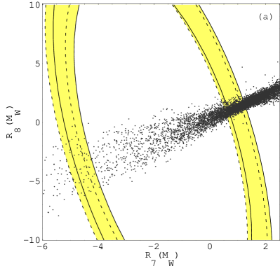
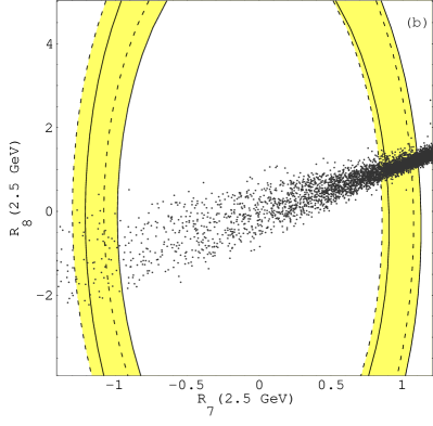
It was recently pointed out in Ref. [8] that the charm mass dependence of the $B\to X_{s}\gamma$ branching ratio was underestimate in all the previous analyses. Indeed, the replacement of the pole mass ($m_{c,pole}/m_{b,pole}=0.29\pm 0.02$) with the $\overline{MS}$ running mass ($m_{c}^{\overline{MS}}(\mu_{b})/m_{b,pole}=0.22\pm 0.04$) increases the branching ratio of about $11\%$. In order to take into account this additional source of uncertainty, we work out the constraints on the Wilson coefficients for both choices of the charm mass; we will then use the loosest bounds in the $b\to s\ell^{+}\ell^{-}$ analysis. We use the numerical expression for the integrated $B\to X_{s}\gamma$ branching ratio as a function of $R_{7,8}(\mu_{W})\equiv C_{7,8}^{\rm tot}(\mu_{W})/C_{7,8}^{\rm SM}(\mu_{W})$ presented in Ref. [7] (Note that, for $m_{c}/m_{b}=0.22$, we had to compute the small corrections to the coefficients $B_{ij}$). For the sake of definiteness we shall take $\mu_{W}=m_{W}$ in deriving the constraints on physics beyond the SM. We impose the bound (4) at ${90\%\ \mathrm{C.L.}}$ and include the theoretical uncertainty due to the variation of the scale $\mu_{b}$ in the range $[m_{b}/2,2m_{b}]$. In Fig. 3a, we present the resulting allowed regions in the $[R_{7}(\mu_{W}),R_{8}(\mu_{W})]$ plane; the solid and dashed lines correspond to the $m_{c}=m_{c,pole}$ and $m_{c}=m_{c}^{\overline{MS}}(\mu_{b})$ cases respectively. According to the analysis presented in Ref. [32], we restrict, in Fig. 3a, to $|R_{8}(\mu_{W})|\leq 10$ in order to satisfy the constraints from the decays $B\to X_{s}g$ and $B\to X_{c\!\!/}$ (where $X_{c\!\!/}$ denotes any hadronic charmless final state). Evolving the allowed regions to the scale $\mu_{b}=2.5\;{\hbox{GeV}}$ and assuming that new physics only enters in $C_{7,8}^{(1)}$, we plot in Fig. 3b the corresponding low–scale bounds in the plane $[R_{7}(2.5\;{\hbox{GeV}}),R_{8}(2.5\;{\hbox{GeV}})]$, where $R_{7,8}(\mu_{b})\equiv A_{7,8}^{\rm tot}(\mu_{b})/A_{7,8}^{\rm SM}(\mu_{b})$. The regions in Fig. 3b translate in the following allowed constraints:

$$\cases{m_{c}/m_{b}=0.29:\;\;\;A_{7}^{\rm tot}(2.5\;{\hbox{GeV}})\in[-0.37,-0.18]\;\&\;[0.21,0.40]\;,&\cr m_{c}/m_{b}=0.22:\;\;\;A_{7}^{\rm tot}(2.5\;{\hbox{GeV}})\in[-0.35,-0.17]\;\&\;[0.25,0.43]\;.&\cr}$$ (42)

In the subsequent numerical analysis we impose the union of the above allowed ranges

$$-0.37\leq A_{7}^{\rm tot,<0}(2.5\;{\hbox{GeV}})\leq-0.17 \& 0.21\leq A_{7}^{\rm tot,>0}(2.5\;{\hbox{GeV}})\leq 0.43$$ (43)

calling them $A_{7}^{\rm tot}$–positive and $A_{7}^{\rm tot}$–negative solutions.

6 Model independent constraints from $b\to s\ell^{+}\ell^{-}$

In this section we compute, in the $[C_{9}^{NP}(\mu_{W}),C_{10}^{NP}]$ plane, the bounds implied by the experimental results given in Eqs. (5)–(11). The results are summarized in Figs. 4–10. In each figure we focus on a different experimental bound and the two plots shown in these figures correspond respectively to the $A_{7}^{\rm tot}$-negative and $A_{7}^{\rm tot}$-positive solutions just discussed. Within each plot we then vary $A_{7}^{\rm tot}$ in the allowed range [given in Eqs. (43)]. The present bounds impact more strongly the decays $B\to(X_{s},K^{*})e^{+}e^{-}$, for which the branching ratios are larger due to the smallness of the electron mass. On the other hand, the decays $B\to K\ell^{+}\ell^{-}$ do not show any enhancement in the low-$\hat{s}$ region and hence they are practically the same for the dielectron and dimuon final states. Hence, the bounds for the $Ke^{+}e^{-}$ and $K\mu^{+}\mu^{-}$ cases are presented in the same plot. In Fig. 10 we combine all the bounds in a single plot. Note that the overall allowed region is driven by the constraints emanating from the decays $B\to X_{s}e^{+}e^{-}$ and $B\to K\mu^{+}\mu^{-}$.

Some comments on the results shown in these figures are in order:

• From the comparison of Figs. 4 and 5, the importance of performing the analysis using the NNLO precision clearly emerges. In Fig. 4 we used the NLO precision ( see for instance in Ref. [33]). In this approximation we have to drop all the finite corrections of order $\alpha_{s}$ (that is all the terms with the superscript $(1)$) and the functions $F_{i}^{(j)}$, $\omega_{7}$ and $\omega_{79}$; we retain the $\omega_{9}$ term in $\tilde{C}_{9}^{\rm eff}$ but drop the corresponding one in $\tilde{C}_{10}^{\rm eff}$. The impact of switching on all these corrections is to lower sizably the branching ratios (this happens both in the full and partial NNLO scenarios previously discussed). As a result, the strong constraints on the new physics Wilson coefficients resulting from the NLO analysis are softened by the inclusion of the NNLO corrections.

• In Fig. 10 we identify four regions still allowed by the constraints on the branching ratios that present very different forward–backward asymmetries. In Fig. 11 we show the shape of the FB asymmetry spectrum for the SM and other three sample points. The distinctive features are the presence or not of a zero and global sign of the asymmetry. A rough indication of the FB asymmetry behavior is thus enough to rule out a large part of the parameter space that the current branching ratios can not explore.

• For the decays $B\to K\mu^{+}\mu^{-}$ and $B\to Ke^{+}e^{-}$, a measurement is now at hand which we have already listed. The BELLE collaboration has combined these branching ratios, getting ${\cal B}(B\to K\ell^{+}\ell^{-})=0.75^{+0.25}_{-0.21}\pm 0.09\times 10^{-6}$ [10]. In showing the constraints in Fig. 7 from $B\to K\ell^{+}\ell^{-}$, we have used this measurement to get the following bounds:

  $$0.38\;\times 10^{-6}\leq{\cal B}(B\to K\ell^{+}\ell^{-})\leq 1.2\;\times 10^{-6}\;{\rm at}\;{90\%\ \mathrm{C.L.}}\;.$$ (44)

Concerning the upper bound, $1.2\times 10^{-6}$, we note that currently a discrepancy exists between the BELLE [10] and the BABAR [11] results, with the latter reporting an upper limit ${\cal B}(B\to K\ell^{+}\ell^{-})<0.5\times 10^{-6}$ (at 90% C.L.) conflicting mildly with the BELLE measurements. However, this could just represent the vagaries of statistical fluctuations, and hopefully this apparent mismatch will be soon resolved with more data. Note that the branching ratio for $B\to K\ell^{+}\ell^{-}$ is bounded both from above and below, resulting in carving out an inner region in the $(C_{9}^{\rm NP}(\mu_{W}),C_{10}^{\rm NP})$ plane.

At the end of this section we present the numerical expressions for the inclusive branching ratios integrated over the low-$\hat{s}$ region only where the full NNLO calculation is at hand. According to the Belle analysis presented in Ref. [10] we choose the integration limits as follows:

$$B\to X_{s}e^{+}e^{-}:\;\left(0.2\;{\hbox{GeV}}\over m_{b}\right)^{2}\leq\hat{s}\leq\left(M_{J/\Psi}-0.6\;{\hbox{GeV}}\over m_{b}\right)^{2}\,,$$ (45)

$$B\to X_{s}\mu^{+}\mu^{-}:\;\left(2m_{\mu}\over m_{b}\right)^{2}\leq\hat{s}\leq\left(M_{J/\Psi}-0.35\;{\hbox{GeV}}\over m_{b}\right)^{2}\;.$$ (46)

The integrated branching ratios have the following form:

$${\cal B}(B\to X_{s}\ell^{+}\ell^{-}) = 10^{-6}\times\Big{[}a_{1}+a_{2}\;|A_{7}^{\rm tot}|^{2}+a_{3}\;(|C_{9}^{\rm NP}|^{2}+|C_{10}^{\rm NP}|^{2})$$ (47)

$$+a_{4}\;{\hbox{Re}}\,A_{7}^{\rm tot}\;{\hbox{Re}}\,C_{9}^{\rm NP}+a_{5}\;{\hbox{Im}}\,A_{7}^{\rm tot}\;{\hbox{Im}}\,C_{9}^{\rm NP}+a_{6}\;{\hbox{Re}}\,A_{7}^{\rm tot}$$

$$+a_{7}\;{\hbox{Im}}\,A_{7}^{\rm tot}+a_{8}\;{\hbox{Re}}\,C_{9}^{\rm NP}+a_{9}\;{\hbox{Im}}\,C_{9}^{\rm NP}+a_{10}\;{\hbox{Re}}\,C_{10}^{\rm NP}\Big{]}\,,$$

where the numerical value of the coefficients $a_{i}$ are given in Table 5 for $\ell=e,\;\mu$. For the integrated branching ratios in the SM we find:

$${\cal B}(B\to X_{s}e^{+}e^{-}) = \left(2.47\pm 0.40\right)\times 10^{-6}\;\;\;(\delta{\cal B}_{X_{s}ee}=\pm 16\%)\;,$$ (48)

$${\cal B}(B\to X_{s}\mu^{+}\mu^{-}) = \left(2.75\pm 0.45\right)\times 10^{-6}\;\;\;(\delta{\cal B}_{X_{s}\mu\mu}=\pm 16\%)\;.$$ (49)

$\ell$	$a_{1}$	$a_{2}$	$a_{3}$	$a_{4}$	$a_{5}$	$a_{6}$	$a_{7}$	$a_{8}$	$a_{9}$	$a_{10}$
$e$	1.9927	6.9357	0.0640	0.5285	0.6574	0.2673	-0.0586	0.4884	0.0095	-0.5288
$\mu$	2.3779	6.9295	0.0753	0.6005	0.7461	0.5955	-0.0600	0.5828	0.0102	-0.6225

Table 5: Numerical values of the coefficients $a_{i}$ (evaluated at $\mu_{b}=5\;{\hbox{GeV}}$) for the decays $B\to X_{s}\ell^{+}\ell^{-}$ ($\ell=e,\;\mu$). $A_{7}^{\rm tot}$ is computed at $\mu_{b}=5\;{\hbox{GeV}}$ while $C_{9}^{\rm NP}$ at $\mu_{W}=m_{W}$ ($C_{10}^{\rm NP}$ is scale independent). We use the full NNLO calculation which is available only in the low–$\hat{s}$ region. The actual ranges for the integrations are chosen according to the Belle analysis presented in Ref. [10]. They are $s\in[4m_{\mu}^{2},(M_{J/\Psi}-0.35\;{\hbox{GeV}})^{2}]$ for the $X_{s}\mu^{+}\mu^{-}$ and $s\in[(0.2\;{\hbox{GeV}})^{2},(M_{J/\Psi}-0.60\;{\hbox{GeV}})^{2}]$ for the $X_{s}e^{+}e^{-}$ modes.

7 Analysis in supersymmetry

In this section we analyze the impact of the $b\to s\gamma$ and $b\to s\ell^{+}\ell^{-}$ experimental constraints on several supersymmetric models. We will first discuss the more restricted framework of the minimal flavour violating MSSM, and then extend the analysis to more general models in which new SUSY flavour changing couplings are allowed to be non–zero for which we will adopt the so–called mass insertion approximation (MIA) [26, 34].

7.1 Minimal Flavour Violation

As already known from the existing literature (see for instance Ref. [35]), minimal flavour violating (MFV) contributions are generally too small to produce sizable effects on the Wilson coefficients $C_{9}$ and $C_{10}$. In the MFV scheme all the genuine new sources of flavour changing transitions other than the CKM matrix are switched off, and the low energy theory depends only on the following parameters: $\mu$, $M_{2}$, $\tan\beta$, $M_{H^{\pm}}$, $M_{\tilde{t}_{2}}$ and $\theta_{\tilde{t}}$ (see Appendix A for a precise definition of the various quantities). Scanning over this parameter space and taking into account the lower bounds on the sparticle masses ($M_{\tilde{t}_{2}}\geq 90\;{\hbox{GeV}}$, $M_{\chi_{i}^{\pm}}\geq 90\;{\hbox{GeV}}$) as well as the $b\to s\gamma$ constraint given in Eq. (4), we derive the ranges for the new physics contributions to $C_{9}$ and $C_{10}$. In order to produce bounds that can be compared with the model independent allowed regions plotted in Fig. 10, we divided the surviving SUSY points in two sets, according to the sign of $A_{7}^{\rm tot}$. Scanning over the following parameter space

$$\cases{M_{\tilde{t}}=90\;{\hbox{GeV}}\div 1\;{\hbox{TeV}}\cr\theta_{\tilde{t}}=-\pi/2\div\pi/2\cr\tan\beta=2.3\div 50\cr\mu=-1\;{\hbox{TeV}}\div 1\;{\hbox{TeV}}\cr M_{2}=0\div 1\;{\hbox{TeV}}\cr M_{H^{\pm}}=78.6\;{\hbox{GeV}}\div 1\;{\hbox{TeV}}\cr M_{\tilde{\nu}}\geq 50\;{\hbox{GeV}}\cr}$$ (50)

we find that the allowed $C_{9}$ and $C_{10}$ ranges are:

$$A_{7}^{\rm tot}<0\Rightarrow\cases{C_{9}^{MFV}(\mu_{W})\in[-0.2,0.4]\,,\cr C_{10}^{MFV}\in[-1.0,0.7]}\,.$$ (51)

$$A_{7}^{\rm tot}>0\Rightarrow\cases{C_{9}^{MFV}(\mu_{W})\in[-0.2,0.3]\,,\cr C_{10}^{MFV}\in[-0.8,0.5]\;.}$$ (52)

We stress that the above discussion applies to any supersymmetric model with flavour universal soft-breaking terms, such as minimal supergravity MSSM and gauge-mediated supersymmetry breaking models. Beyond-the-SM flavour violations in such models are induced only via renormalization group running, and are tiny. Hence, they can be described by MFV models discussed in this paper.

Before finishing this subsection and starting our discussion on models with new flavour changing interactions, let us show in more detail the impact of $b\to s\gamma$ on MFV models. The scatter plot presented in Fig. 3 is obtained varying the MFV SUSY parameters according to the above ranges and shows the strong correlation between the values of the Wilson coefficients $C_{7}$ and $C_{8}$. In fact, the SUSY contributions to the magnetic and chromo–magnetic coefficients differ only because of colour factors and loop-functions. In Figs. 12 and 13 we present the dependence of the charged Higgs and chargino contributions to $C_{7}$ on the relevant mass parameters (that are the charged Higgs mass for the former and the lightest chargino and stop masses for the latter). Note that we plot the SUSY Wilson coefficients at the scale $\mu_{b}$ normalized to the SM values. In the chargino case we are able to exploit the $\theta_{\tilde{t}}$ and $\tan\beta$ dependence since (for non negligible values of the stop mixing angle) the chargino contribution is essentially proportional to $\sin\theta_{\tilde{t}}\tan\beta$. Indeed, the various curves are very stable with respect to variations of $\tan\beta$ and $\theta_{\tilde{t}}$ according to the ranges specified in Eq. (50); in order not to complicate unnecessarily the figure we show the actual spread for the $M_{\chi}=200\;{\hbox{GeV}}$ case only (note that according to the above discussion we require $|\theta_{\tilde{t}}|\geq 0.01$). In order to show the full strength of these figures let us entertain a scenario in which $C_{7}$ has the same sign as in the SM. In this situation large contributions to $C_{7}$ are completely ruled out. This means that, looking at Figs. 12 and 13, it is possible to obtain lower bounds on some SUSY particles. Note that Fig. 13 has very strong consequences. Assuming for instance $M_{\tilde{t}_{2}}=M_{\chi}=500\;{\hbox{GeV}}$ we see that the ratio $R_{7}^{\chi}/(\sin\theta_{\tilde{t}}\tan\beta)$ is of order 0.2. If we then allow for larger values of the stop mixing angle and of $\tan\beta$, the contribution can easily violate the $b\to s\gamma$ constraint by more than one order of magnitude (e.g. for $\sin\theta_{\tilde{t}}=0.5$ and $\tan\beta=50$ we obtain something of order 6 that is orders of magnitude above the current limit).

7.2 Gluino contributions

Gluino contributions to $C_{9}$ and $C_{10}$ are governed by mass insertions in the down squark mass matrix. From the analysis presented in Ref. [35] we see that the dominant diagrams involve the parameter $(\delta^{d}_{23})_{LL}$ and that large deviations from the SM are unlikely. The impact of $(\delta^{d}_{23})_{LR}$ is negligible for the following two reasons. First of all, contributions to either $C_{9}$ or $C_{10}$ are obtained by $b_{L}\to s_{L}$ transitions and LR insertions can therefore enter only at the second order in the mass insertion expansion. More importantly, the insertion $(\delta^{d}_{23})_{LR}$ gives a contribution to the coefficient $C_{7}$ that is two orders of magnitude bigger than the SM one. The bottom line of this discussion is that $(\delta^{d}_{23})_{LR}$ contributions to the semileptonic Wilson coefficients are extremely suppressed. Moreover, there are no gluino box diagrams and the $\gamma$–penguins are enhanced with respect to the $Z$–ones so that only contributions to $C_{9}$ are non vanishing. Their explicit expression is (see Ref. [35] for the analytical equations):

$$C_{9}^{\tilde{g},MI}=-0.93\left(250{\hbox{GeV}}\over M_{\tilde{q}}\right)^{2}{f_{8}^{MI}(x_{\tilde{g}\tilde{q}})\over 1/3}(\delta^{d}_{23})_{LL}\,,$$ (53)

where $x_{\tilde{g}\tilde{q}}=M_{\tilde{g}}^{2}/M_{\tilde{q}}^{2}$, the $f_{8}^{MI}(x)$ loop-function is always smaller than $1/3$ and can be found in Appendix C. The situation is thus similar to the MFV case and the same conclusions hold.

7.3 Chargino contributions: Extended–MFV models

A basically different scenario arises if chargino–mediated penguin and box diagrams are considered. As can be inferred by Table 4 in Ref. [35], the presence of a light $\tilde{t}_{2}$ generally gives rise to large contributions to $C_{9}$ and especially to $C_{10}$. In the following, we will concentrate on the so–called Extended MFV (EMFV) models that the two of us described in Ref. [36] and that we will briefly summarize below. In these models we can fully exploit the impact of chargino penguins with a light $\tilde{t}$ still working with a limited number of free parameters.

EMFV models are based on the heavy squarks and gluino assumption. In this framework, the charged Higgs and the lightest chargino and stop masses are required to be heavier than $100\;{\hbox{GeV}}$ in order to satisfy the lower bounds from direct searches. The rest of the SUSY spectrum is assumed to be almost degenerate and heavier than $1\;{\hbox{TeV}}$. The lightest stop is almost right–handed and the stop mixing angle (which parameterizes the amount of the left-handed stop $\tilde{t}_{L}$ present in the lighter mass eigenstate) turns out to be of order $O(m_{W}/M_{\tilde{q}})\simeq 10\%$; for definiteness we will take $|\theta_{\tilde{t}}|\leq\pi/10$. The assumption of a heavy ($\geq 1$ TeV) gluino totally suppresses any possible gluino–mediated SUSY contribution to low energy observables. Note that even in the presence of a light gluino (i.e. $M_{\tilde{g}}\simeq O(300\;{\hbox{GeV}})$) these penguin diagrams remain suppressed due to the heavy down squarks present in the loop. In the MIA approach, a diagram can contribute sizably only if the inserted mass insertions involve the light stop. All the other diagrams require necessarily a loop with at least two heavy ($\geq 1\;{\hbox{TeV}}$) squarks and are therefore automatically suppressed. This leaves us with only two unsuppressed flavour changing sources other than the CKM matrix, namely the mixings $\tilde{u}_{L}-\tilde{t}_{2}$ (denoted by $\delta_{\tilde{u}_{L}\tilde{t}_{2}}$) and $\tilde{c}_{L}-\tilde{t}_{2}$ (denoted by $\delta_{\tilde{c}_{L}\tilde{t}_{2}}$). We note that $\delta_{\tilde{u}_{L}\tilde{t}_{2}}$ and $\delta_{\tilde{c}_{L}\tilde{t}_{2}}$ are mass insertions extracted from the up–squarks mass matrix after the diagonalization of the stop system and are therefore linear combinations of $(\delta_{13})^{U}_{LR}$, $(\delta_{13})^{U}_{LL}$ and of $(\delta_{23})^{U}_{LR}$, $(\delta_{23})^{U}_{LL}$, respectively. The insertions relevant to our discussion are normalized as follows:

$$\delta_{\tilde{u}(\tilde{c})_{L}\tilde{t}_{2}}\equiv{M^{2}_{\tilde{u}(\tilde{c})_{L}\tilde{t}_{2}}\over M_{\tilde{t}_{2}}M_{\tilde{q}}}{|V_{td(s)}|\over V_{td(s)}^{*}}\;.$$ (54)

The phenomenological impact of $\delta_{\tilde{t}_{2}\tilde{u}_{L}}$ has been studied in Ref. [36] and its impact on the $b\to s\gamma$ and $b\to s\ell^{+}\ell^{-}$ transitions is indeed negligible. Therefore, we are left with the MIA parameter $\delta_{\tilde{t}_{2}\tilde{c}_{L}}$ only. Thus, the SUSY parameter space that we have to deal with is: $\mu$, $M_{2}$, $\tan\beta$, $M_{\tilde{t}_{2}}$, $\sin\theta_{\tilde{t}}$, $M_{H^{\pm}}$, $M_{\tilde{\nu}}$ and $\delta_{\tilde{t}_{2}\tilde{c}_{L}}$.

The explicit expressions for the mass insertion contributions to the Wilson coefficients $C_{7}$ – $C_{10}$ are summarized in Appendix B.

In order to explore the region in the $[C_{9}^{NP},C_{10}^{NP}]$ plane (where $C_{9,10}^{NP}$ are the sum of MFV and MI contributions and are explicitly defined in Appendix B) that is accessible to these models, we performed a high statistic scanning over the following EMFV parameter space requiring each point to survive the constraints coming from the sparticle masses lower bounds and $b\to s\gamma$:

$$\cases{M_{\tilde{t}}=90\;{\hbox{GeV}}\div 1\;{\hbox{TeV}}\cr\theta_{\tilde{t}}=-\pi/10\div\pi/10\cr\tan\beta=2.3\div 50\cr\mu=-1\;{\hbox{TeV}}\div 1\;{\hbox{TeV}}\cr M_{2}=0\div 1\;{\hbox{TeV}}\cr M_{H^{\pm}}=78.6\;{\hbox{GeV}}\div 1\;{\hbox{TeV}}\cr M_{\tilde{\nu}}\geq 50\;{\hbox{GeV}}\cr\delta_{\tilde{t}_{2}\tilde{c}_{L}}=-1\div 1\;.\cr}$$ (55)

The surviving points are shown in Fig. 10 together with the model independent constraints. Note that these SUSY models can account only for a small part of the region allowed by the model independent analysis of current data. We stress that in our numerical analysis reported here, we have used the integrated branching ratios to put constraints on the effective coefficients. This procedure allows multiple solutions, which can be disentangled from each other only with the help of both the dilepton mass spectrum and the forward-backward asymmetry. Only such measurements would allow us to determine the exact values and signs of the Wilson coefficients $C_{7}$, $C_{9}$ and $C_{10}$.

8 Summary

We have presented theoretical branching ratios for the rare $B$ decays $B\to X_{s}\ell^{+}\ell^{-}$ and $B\to(K,K^{*})\ell^{+}\ell^{-}$, incorporating the NNLO contributions in the former and partial NNLO improvements in the latter. This has allowed us to carry out a theoretical analysis of the radiative decays $B\to X_{s}\gamma$ and the mentioned semileptonic decays to the same order in $\alpha_{s}$. In addition, we have included the leading power corrections in $1/m_{b}$ and $1/m_{c}$ in the inclusive decays. The dilepton invariant mass spectrum is calculated in the NNLO precision in the low dilepton invariant mass region, $\hat{s}<0.25$. The spectrum for $\hat{s}>0.25$ calculated to the same theoretical accuracy is not yet available. We estimate the spectrum in this range from the known partial NNLO, by noting that the dilepton mass spectrum in the full NNLO is close to the partial NNLO spectrum in the range $\hat{s}<0.25$ for the choice of the scale $\mu_{b}=2.5$ GeV. Following this observation, we use the partial NNLO spectrum with this scale to estimate the central value of the full NNLO spectrum for $\hat{s}>0.25$. The branching ratios in the NNLO accuracy in the SM are calculated to have the values ${\cal B}(B\to X_{s}e^{+}e^{-})=(6.89\pm 1.01)\times 10^{-6}$ and ${\cal B}(B\to X_{s}\mu^{+}\mu^{-})=(4.15\pm 0.7)\times 10^{-6}$. They are lower by typically 12% and 20%, respectively, compared to their NLO estimates for the central values of the input parameters, and are approximately a factor 2 to 4 away from their respective experimental upper limits. Hence, current B factory experiments will soon probe these decays at the level of the SM sensitivity. In view of the fact that the dilepton mass spectrum is calculated to the NNLO accuracy only for $\hat{s}<0.25$, and the long-distance effects are not expected to be dominant, we stress the need to measure the inclusive decays $B\to X_{s}\ell^{+}\ell^{-}$ in this dilepton mass range. In fact, as shown in this paper, such a measurement is theoretically as robust as the inclusive radiative decay $B\to X_{s}\gamma$.

In the second part of this paper, we have used our improved theoretical calculations to extract from the current data, listed in Eqs. (4) – (11), the allowed ranges of the effective Wilson coefficients $C_{7}(\mu)$ – $C_{10}(\mu)$. In doing this, we have first determined the ranges on the Wilson coefficients $C_{7}(\mu)$ and $C_{8}(\mu)$ from $B\to X_{s}\gamma$ decay, and then determined the allowed ranges of the coefficients $C_{9}^{NP}(\mu_{W})$ and $C_{10}^{NP}$ (at 90% C.L.). Since the decays $B\to K\ell^{+}\ell^{-}$ are now measured by the BELLE collaboration, they carve out an inner region in the ($C_{9}^{NP}(\mu_{W})$,$C_{10}^{NP}$) plane, allowed previously. Under the assumption that the SM-operator basis of the effective Hamiltonian is sufficient to incorporate also the beyond-the-SM physics effects, the analysis presented in this paper is model independent. We find that all current data are consistent with the SM. However, present experimental measurements allow considerable room for beyond-the-SM effects, which we have worked out in specific supersymmetric contexts. For this purpose, we have used the MFV model, and an Extended-MFV model introduced in Ref. [36]. The resulting constraints on the supersymmetric parameters are worked out, in particular on the charged Higgs mass, $M_{H^{\pm}}$, the lighter of the two stop masses, $M_{\tilde{t}_{2}}$, the ratio of the two Higgs vacuum expectation values, $\tan\beta$, and the MIA parameter $(\delta_{23})$. With more data, expected from the leptonic and hadronic $B$ factories, these constraints will become either much more stringent, pushing the supersymmetric frontier further, or else, more optimistically, new data may lead to impeccable evidence for new physics effects. We have illustrated this using the forward-backward asymmetry in $B\to X_{s}\ell^{+}\ell^{-}$ decays.

9 Acknowledgments

We would like to thank Wulfrin Bartel, Ed Thorndike, Mikihiko Nakao, Hiro Tajima, Vera Lüth and Howie Haber for helpful discussions and communications on the data. We also thank Patricia Ball for a helpful correspondence on the exclusive decay form factors. C.G. and G.H. would like to thank the DESY theory group for warm hospitality during their stay in Hamburg, where numerous stimulating discussion regarding this work took place. E.L. acknowledges financial support from the Alexander von Humboldt Foundation. The work of C. G. was partially supported by Schweizerischer Nationalfonds. The work of G. H. was supported by the Department of Energy, Contract DE-AC03-76SF00515.

Appendix A Stop and chargino mass matrices

The $2\times 2$ stop mass matrix is given by

$$M^{2}_{\tilde{t}}=\pmatrix{M^{2}_{\tilde{t}_{LL}}&M^{2}_{\tilde{t}_{LR}}\cr M^{2*}_{\tilde{t}_{LR}}&M^{2}_{\tilde{t}_{RR}}\cr}\,,$$ (56)

where

$$M^{2}_{\tilde{t}_{LL}} = M^{2}_{\tilde{q}}+({1\over 2}-{2\over 3}\sin^{2}\theta_{W})\cos 2\beta\,m_{Z}^{2}+m_{t}^{2}\enspace,$$ (57)

$$M^{2}_{\tilde{t}_{RR}} = M^{2}_{\tilde{q}}+{2\over 3}\sin^{2}\theta_{W}\cos 2\beta\,m_{Z}^{2}+m_{t}^{2}\enspace,$$ (58)

$$M^{2}_{\tilde{t}_{LR}} = m_{t}(A_{t}-\mu^{*}\cot\beta)\enspace.$$ (59)

The eigenvalues are given by

$$2M^{2}_{\tilde{t}_{1},\tilde{t}_{2}}=(M^{2}_{\tilde{t}_{LL}}+M^{2}_{\tilde{t}_{RR}})\pm\sqrt{(M^{2}_{\tilde{t}_{LL}}-M^{2}_{\tilde{t}_{RR}})^{2}+4(M^{2}_{\tilde{t}_{LR}})^{2}}\enspace,$$ (60)

with $M^{2}_{\tilde{t}_{2}}\leq M^{2}_{\tilde{t}_{1}}$. We parametrize the mixing matrix ${\mathcal{R}}^{\tilde{t}}$ so that

$$\pmatrix{\tilde{t}_{1}\cr\tilde{t}_{2}}={\mathcal{R}}^{\tilde{t}}\left(\begin{array}[]{c}\tilde{t}_{L}\\ \tilde{t}_{R}\end{array}\right)=\left(\begin{array}[]{cc}\cos\theta_{\tilde{t}}&+\sin\theta_{\tilde{t}}\\ -\sin\theta_{\tilde{t}}&\cos\theta_{\tilde{t}}\end{array}\right)\left(\begin{array}[]{c}\tilde{t}_{L}\\ \tilde{t}_{R}\end{array}\right)\enspace.$$ (61)

The chargino mass matrix

$$M^{\tilde{\chi}^{+}}_{\alpha\beta}=\left(\begin{array}[]{cc}M_{2}&m_{W}\sqrt{2}\sin\beta\\ m_{W}\sqrt{2}\cos\beta&\mu\end{array}\right)\,,$$ (62)

can be diagonalized by the bi-unitary transformation

$$\tilde{U}^{*}_{j\alpha}M^{\tilde{\chi}^{+}}_{\alpha\beta}\tilde{V}^{*}_{k\beta}=M_{\tilde{\chi}_{j}^{+}}\delta_{jk}\enspace,$$ (63)

where $\tilde{U}$ and $\tilde{V}$ are unitary matrices such that $M_{\tilde{\chi}_{j}^{+}}$ are positive and $M_{\tilde{\chi}_{1}^{+}}<M_{\tilde{\chi}_{2}^{+}}$.

Appendix B Wilson coefficients $C_{7}$ – $C_{10}$ in EMFV models

In this appendix we collect the explicit expressions for the Wilson coefficients $C_{7}$ – $C_{10}$ in the mass insertion approximation. The conventions for the definition of the chargino mass matrix is summarized in Appendix A, the normalization of the mass insertion is given in Eq. (54) in the text, and the loop functions encountered below can be found in Appendix C.

• Contributions to the magnetic and chromo–magnetic dipole moment coefficients:

$$C_{7,8}^{MI} = {\delta_{\tilde{t}_{2}\tilde{c}_{L}}\over 6}\left|V_{cs}\over V_{ts}\right|{m_{W}^{2}\over M_{\tilde{q}}^{2}}{M_{\tilde{t}_{2}}\over M_{\tilde{q}}}\sum_{i=1}^{2}V_{i1}\Bigg{[}\left(\sin\theta_{\tilde{t}}V_{i1}^{*}-{m_{t}\cos\theta_{\tilde{t}}\over\sqrt{2}\sin\beta m_{W}}V_{i2}^{*}\right)f_{1,3}^{\rm MI}(x_{i},x_{\tilde{t}_{2}})+$$ (64)

$$\sin\theta_{\tilde{t}}U_{i2}^{*}{\sqrt{2}M_{\chi_{i}}\over m_{W}\cos\beta}f_{2,4}^{\rm MI}(x_{i},x_{\tilde{t}_{2}})\Bigg{]}\;.$$

The contributions to the semileptonic coefficients can be divided in three classes:

• Photon mediated penguin diagrams:

  $$C_{10}^{MI,\gamma} = 0\;,$$ (65)

  $$C_{9}^{MI,\gamma} = {1\over 9}\delta_{\tilde{t}_{2}\tilde{c}_{L}}\left|V_{cs}\over V_{ts}\right|{m_{W}^{2}\over M_{\tilde{q}}^{2}}{M_{\tilde{t}_{2}}\over M_{\tilde{q}}}\sum_{i=1}^{2}V_{i1}\left({m_{t}\cos\theta_{\tilde{t}}\over\sqrt{2}\sin\beta m_{W}}V_{i2}^{*}-\sin\theta_{\tilde{t}}V_{i1}^{*}\right)f_{7}^{\rm MI}(x_{i},x_{\tilde{t}_{2}})\;.$$ (66)

• Z mediated penguin diagrams:

  $$C_{10}^{MI,Z} = {\delta_{\tilde{t}_{2}\tilde{c}_{L}}\over 4\sin^{2}\theta_{W}}\left|V_{cs}\over V_{ts}\right|{M_{\tilde{t}_{2}}\over M_{\tilde{q}}}\sum_{i,j,=1}^{2}V_{i1}\Bigg{\{}\left(\sin\theta_{\tilde{t}}V_{j1}^{*}-{m_{t}\cos\theta_{\tilde{t}}\over\sqrt{2}\sin\beta m_{W}}V_{j2}^{*}\right)$$ (67)

  $$\hskip-62.59596pt\times\left(U_{i1}^{*}U_{j1}{M_{\chi_{i}}M_{\chi_{j}}\over M_{\tilde{q}}M_{\tilde{t}_{2}}}j(x_{i},x_{j},x_{\tilde{t}_{2}})+V_{i1}^{*}V_{j1}{k(x_{i},x_{j},x_{\tilde{t}_{2}})\over 2x_{\tilde{t}_{2}}}-\delta_{ij}V_{i1}V_{i2}^{*}{k(x_{i},x_{\tilde{t}_{2}},1)\over 2x_{\tilde{t}_{2}}}\right)$$

  $$\hskip-62.59596pt-\sin\theta_{\tilde{t}}V_{j1}^{*}\;\delta_{ij}V_{i1}V_{i2}^{*}{k(x_{i},x_{\tilde{t}_{2}},1)\over 2x_{\tilde{t}_{2}}}\Bigg{\}}\;,$$

  $$C_{9}^{MI,Z} = (4\sin^{2}\theta_{W}-1)C_{10}^{MI,Z}\;.$$ (68)

• Box diagrams with an internal sneutrino line:

  $$C_{10}^{MI,box} = {\delta_{\tilde{t}_{2}\tilde{c}_{L}}\over\sin^{2}\theta_{W}}\left|V_{cs}\over V_{ts}\right|{m_{W}^{2}\over M_{\tilde{q}}^{2}}{M_{\tilde{t}_{2}}\over M_{\tilde{q}}}\sum_{i,j=1}^{2}|V_{i1}|^{2}V_{j1}\left({m_{t}\cos\theta_{\tilde{t}}\over\sqrt{2}\sin\beta m_{W}}V_{j2}^{*}-\sin\theta_{\tilde{t}}V_{j1}^{*}\right)$$ (69)

  $$\times d_{2}^{\rm MI}(x_{i},x_{j},x_{\tilde{t}_{2}},x_{\tilde{\nu}})\;,$$

  $$C_{9}^{MI,box} = -C_{10}^{MI,box}\;.$$ (70)

The branching ratios for the various decays are obtained from Eqs. (14)–(15) by means of the following replacement:

$$C_{7,8}^{NP} \rightarrow C_{7,8}^{MFV}+C_{7,8}^{MI}\;,$$ (71)

$$C_{9,10}^{NP} \rightarrow C_{9,10}^{MFV}+C_{9,10}^{MI,\gamma}+C_{9,10}^{MI,Z}+C_{9,10}^{MI,box}\;,$$ (72)

where the expressions for $C_{i}^{MFV}$ can be found in Ref. [33].

Appendix C Loop functions

The various loop functions introduced in Appendix B are listed below.

$$f_{1}(x) = {-7+12x+3x^{2}-8x^{3}+6x(-2+3x)\log x\over 6(x-1)^{4}}\;,$$ (73)

$$f_{2}(x) = {5-12x+7x^{2}-2x(-2+3x)\log x\over 2(x-1)^{3}}\;,$$ (74)

$$f_{3}(x) = {2+3x-6x^{2}+x^{3}+6x\log x\over 6(x-1)^{4}}\;,$$ (75)

$$f_{4}(x) = {-1+x^{2}-2x\log x\over 2(x-1)^{3}}\;,$$ (76)

$$f_{i}^{MI}(x,y) = {f_{i}(1/x)-f_{i}(y/x)\over x(1-y)}\;\;\;\;(i=1,2,3,4)\;.$$ (77)

$$f_{7}(x) = {52-153x+144x^{2}-43x^{3}+6(6-9x+2x^{3})\log x\over 6(x-1)^{4}}\;,$$ (78)

$$f_{8}(x) = {2-9x+18x^{2}-11x^{3}+6x^{3}\log x\over(x-1)^{4}}\;,$$ (79)

$$f_{i}^{MI}(x,y) = {f_{i}(x)-f_{i}(x/y)\over 1-y}\;\;\;\;(i=7,8)\;.$$ (80)

$$j(x) = {x\log x\over x-1}\;,\;\;\;\;j(x,y)={j(x)-j(y)\over x-y}\;,\;\;\;\;j(x,y,z)={j(x,z)-j(y,z)\over x-y}\;,$$ (81)

$$k(x) = {x^{2}\log x\over x-1}\;,\;\;\;\;k(x,y)={k(x)-k(y)\over x-y}\;,\;\;\;\;k(x,y,z)={k(x,z)-k(y,z)\over x-y}\;.$$ (82)

$$d_{2}(x,y,z,t) = -{1\over 4}\left[{x\log x\over(x-y)(x-z)(x-t)}+(x\leftrightarrow y)+(x\leftrightarrow z)+(x\leftrightarrow t)\right]\;,$$ (83)

$$d_{2}^{MI}(x,y,z,t) = {d_{2}(x,y,1,t)-d_{2}(x,y,z,t)\over 1-z}\;.$$ (84)

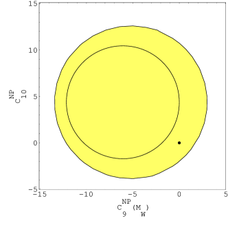
Figure 1: Relative size $R(\hat{s})$ of the combined $1/m_{b}$ and $1/m_{c}$ power corrections as defined in Eq. (34) in the decay rate in $B\to X_{s}\ell^{+}\ell^{-}$ decays as a function of the dilepton invariant mass in the SM (solid) and for $C_{7}=-C_{7}^{SM}$ (dashed).

Figure 2: Partial (dashed lines) vs full (solid lines) NNLO computation of the branching ratio $B\to X_{s}e^{+}e^{-}$. In the left plot ($\hat{s}\in[0,0.05]$) the lowest curves are for $\mu=10\;{\hbox{GeV}}$ and the uppermost ones for $\mu=2.5\;{\hbox{GeV}}$. In the right plot the $\mu$ dependence is reversed: the uppermost curves correspond to $\mu=10\;{\hbox{GeV}}$ and the lowest ones to $\mu=2.5\;{\hbox{GeV}}$. The right-hand plot also holds for the decay $B\to X_{s}\mu^{+}\mu^{-}$.

Figure 3: ${90\%\ \mathrm{C.L.}}$ bounds in the $[R_{7}(\mu),R_{8}(\mu)]$ plane following from the world average $B\to X_{s}\gamma$ branching ratio for $\mu=m_{W}$ (left-hand plot) and $\mu=2.5$ GeV (right-hand plot). Theoretical uncertainties are taken into account. The solid and dashed lines correspond to the $m_{c}=m_{c,pole}$ and $m_{c}=m_{c}^{\overline{MS}}(\mu_{b})$ cases respectively. The scatter points correspond to the expectation in MFV models (the ranges of the SUSY parameters are specified in the text).

Figure 4: NLO Case. Constraints in the $[C_{9}^{NP}(\mu_{W}),C_{10}^{NP}]$ plane that come from the BELLE ${90\%\ \mathrm{C.L.}}$ upper limit ${\cal B}(B\to X_{s}e^{+}e^{-})\leq 10.1\times 10^{-6}$. Theoretical uncertainties are taken into account. The plots correspond to the $A_{7}^{\rm tot}(2.5\;{\hbox{GeV}})<0$ and $A_{7}^{\rm tot}(2.5\;{\hbox{GeV}})>0$ case, respectively. In each plot the outer contour corresponds to the smaller $|A_{7}^{\rm tot}|$ value. The dot in plot on the left is the SM point.

Figure 5: NNLO Case. Constraints in the $[C_{9}^{NP}(\mu_{W}),C_{10}^{NP}]$ plane that come from the BELLE ${90\%\ \mathrm{C.L.}}$ upper limit ${\cal B}(B\to X_{s}e^{+}e^{-})\leq 10.1\times 10^{-6}$. See Fig. 4 for further details.

Figure 6: NNLO Case. Constraints in the $[C_{9}^{NP}(\mu_{W}),C_{10}^{NP}]$ plane that come from the BELLE ${90\%\ \mathrm{C.L.}}$ upper limit ${\cal B}(B\to X_{s}\mu^{+}\mu^{-})\leq 19.1\times 10^{-6}$. See Fig. 4 for further details.

Figure 7: NNLO Case. Constraints in the $[C_{9}^{NP}(\mu_{W}),C_{10}^{NP}]$ plane that come from the $90\%CL$ BELLE constraints $0.38\times 10^{-6}\leq{\cal B}(B\to K\ell^{+}\ell^{-})\leq 1.2\times 10^{-6}$ (Eq. 7). Note that only the annular regions between the two circles is allowed. See Fig. 4 for further details.

Figure 8: NNLO Case. Constraints in the $[C_{9}^{NP}(\mu_{W}),C_{10}^{NP}]$ plane that come from the $90\%CL$ BELLE constraint ${\cal B}(B\to K^{*}\mu^{+}\mu^{-})\leq 3.0\times 10^{-6}$. See Fig. 4 for further details.

Figure 9: NNLO Case. Constraints in the $[C_{9}^{NP}(\mu_{W}),C_{10}^{NP}]$ plane that come from the $90\%CL$ BELLE constraint ${\cal B}(B\to K^{*}e^{+}e^{-})\leq 5.1\times 10^{-6}$. See Fig. 4 for further details.

Figure 10: NNLO Case. Superposition of all the constraints. The plots correspond to the $A_{7}^{\rm tot}(2.5\;{\hbox{GeV}})<0$ and $A_{7}^{\rm tot}(2.5\;{\hbox{GeV}})>0$ case, respectively. The points are obtained by means of a scanning over the EMFV parameter space and requiring the experimental bound from $B\to X_{s}\gamma$ to be satisfied.

Figure 11: Differential Forward–Backward asymmetry for the decay $B\to X_{s}\ell^{+}\ell^{-}$. The four curves correspond to the points indicated in Fig. 10.

Figure 12: Dependence of $R_{7}^{H^{\pm}}(\mu_{b})\equiv C_{7}^{H^{\pm}}(\mu_{b})/C_{7}^{\rm SM}(\mu_{b})$ on the mass of the charged Higgs.

Figure 13: Dependence of $R_{7}^{\chi}(\mu_{b})\equiv C_{7}^{\chi}(\mu_{b})/C_{7}^{\rm SM}(\mu_{b})$ on the mass of the lightest stop in MFV models. The chargino contribution is essentially proportional to $\sin\theta_{\tilde{t}}\tan\beta$ for not too small $\sin\theta_{\tilde{t}}$. For the set of curves 2 we show the variation due to several choices of $\theta_{\tilde{t}}$ and $\tan\beta$. The thick bunch of lines is obtained for $(\sin\theta_{\tilde{t}},\tan\beta)=(0.025,40)$, $(0.05,20)$, $(0.1,10)$, $(0.2,5)$, $(.5,2)$ for which $\sin\theta_{\tilde{t}}\tan\beta=1$. The two thin curves correspond to $(\sin\theta_{\tilde{t}},\tan\beta)=(0.1,20)$ and $(.1,40)$, with the product $\sin\theta_{\tilde{t}}\tan\beta$ having a value 2 and 4, respectively.

References

• [1] M.Β S.Β Alam et al. [CLEO Collaboration], Phys.Β Rev.Β Lett.Β  74 (1995) 2885.
• [2] See, e.g., C.Β Greub, talk given at the 8th International Symposium on Heavy Flavour Physics, Southampton, England, 25-29 Jul 1999. [hep-ph/9911348].
• [3] S. Chen et al. [CLEO Collaboration], Phys.Β Rev.Β Lett.Β  87 (2001) 251807 [hep-ex/0108032].
• [4] R.Β Barate etΒ al. [ALEPH Collaboration], Phys. Lett. B 429 (1998) 169.
• [5] K.Β Abe et al. [BELLE Collaboration], Phys.Β Lett.Β B 511 (2001) 151 [hep-ex/0103042].
• [6] K.Β Chetyrkin, M.Β Misiak and M.Β MΓΌnz, Phys.Β Lett.Β B 400, 206 (1997) [Erratum-ibid.Β B 425, 414 (1997)] [hep-ph/9612313].
• [7] A.Β L.Β Kagan and M.Β Neubert, Eur.Β Phys.Β J.Β C 7, 5 (1999) [hep-ph/9805303].
• [8] P.Β Gambino and M.Β Misiak, Nucl.Β Phys.Β B 611 (2001) 338 [hep-ph/0104034].
• [9] L.Β Everett et al., preprint CERN-TH-2001-354 [hep-ph/0112126].
• [10] K.Β Abe et al. [BELLE Collaboration], BELLE-CONF-0110 [hep-ex/0107072];
K.Β Abe et al. [BELLE Collaboration], Phys.Β Rev.Β Lett.Β  88 (2002) 021801 [hep-ex/0109026].
• [11] B.Β Aubert et al. [BABAR Collaboration], BABAR-CONF-01/24, SLAC-PUB-8910 [hep-ex/0107026] and BABAR-PUB-01/19, SLAC-PUB-9102 [hep-ex/0201008].
• [12] T.Β Affolder et al. [CDF Collaboration], Phys.Β Rev.Β Lett.Β  83 (1999) 3378 [hep-ex/9905004].
• [13] S.Β Anderson et al. [CLEO Collaboration], Phys.Β Rev.Β Lett.Β  87 (2001) 181803 [hep-ex/0106060].
• [14] A.Β Ali, G.Β Hiller, L.Β T.Β Handoko and T.Β Morozumi, Phys.Β Rev.Β D 55 (1997) 4105 [hep-ph/9609449].
• [15] A.Β Ali, P.Β Ball, L.Β T.Β Handoko and G.Β Hiller, Phys.Β Rev.Β D 61 (2000) 074024 [hep-ph/9910221].
• [16] C.Β Bobeth, M.Β Misiak and J.Β Urban, Nucl.Β Phys.Β B 574 (2000) 291 [hep-ph/9910220].
• [17] H.Β H.Β Asatrian, H.Β M.Β Asatrian, C.Β Greub and M.Β Walker, Phys.Β Lett.Β B 507 (2001) 162 [hep-ph/0103087];
H.Β H.Β Asatryan, H.Β M.Β Asatrian, C.Β Greub and M.Β Walker, Phys.Β Rev.Β D 65 (2002) 074004 [hep-ph/0109140].
• [18] A.Β Ali and G.Β Hiller, Eur.Β Phys.Β J.Β C 8, 619 (1999) [hep-ph/9812267].
• [19] G.Β Buchalla, G.Β Isidori and S.Β J.Β Rey, Nucl.Β Phys.Β B 511, 594 (1998) [hep-ph/9705253].
• [20] A.Β Ali and A.Β Y.Β Parkhomenko, Eur.Β Phys.Β J.Β C 23 (2002) 89 [hep-ph/0105302].
• [21] M.Β Beneke, T.Β Feldmann and D.Β Seidel, Nucl.Β Phys.Β B 612 (2001) 25 [hep-ph/0106067].
• [22] S.Β W.Β Bosch and G.Β Buchalla, Nucl.Β Phys.Β B 621 (2002) 459 [hep-ph/0106081].
• [23] H. Tajima [BELLE Collaboration], Plenary Talk, XX International Symposium on Lepton and Photon Interactions at High Energies, July 23 - 28, 2001, Rome.
• [24] B. Aubert et al. [BABAR Collaboration] Phys.Β Rev.Β Lett.Β  88 (2002) 101805 [hep-ex/0110065].
• [25] M.Β Ciuchini, G.Β Degrassi, P.Β Gambino and G.Β F.Β Giudice, Nucl.Β Phys.Β B 534 (1998) 3 [hep-ph/9806308].
• [26] L.Β J. Hall, V.Β A. Kostelecky, and S.Β Raby, Nucl. Phys.Β B 267 (1986) 415.
• [27] J.Β L.Β Hewett and J.Β D.Β Wells, Phys.Β Rev.Β D 55, 5549 (1997) [hep-ph/9610323].
• [28] N.Β Cabibbo, Phys. Rev. Lett. 10, 531 (1963),
M. Kobayashi and T. Maskawa, Prog. Theor. Phys. 49, 652 (1973).
• [29] M.Β Misiak, Nucl. Phys. B 393 (1993) 23 and B 439 (1995) 461.
• [30] J.Β Chay, H.Β Georgi and B.Β Grinstein, Phys.Β Lett.Β B 247, 399 (1990); I.Β I.Β Bigi, N.Β G.Β Uraltsev and A.Β I.Β Vainshtein, Phys.Β Lett.Β B 293, 430 (1992) [Erratum-ibid.Β B 297, 477 (1992)] [hep-ph/9207214]; B.Β Blok, L.Β Koyrakh, M.Β A.Β Shifman and A.Β I.Β Vainshtein, Phys.Β Rev.Β D 49, 3356 (1994) [Erratum-ibid.Β D 50, 3572 (1994)] [hep-ph/9307247].
• [31] J.Β Charles, A.Β Le Yaouanc, L.Β Oliver, O.Β Pene and J.Β C.Β Raynal, Phys.Β Lett.Β B 451 (1999) 187 [hep-ph/9901378].
• [32] C.Β Greub and P.Β Liniger, Phys.Β Rev.Β D 63 (2001) 054025 [hep-ph/0009144].
• [33] P.Β L.Β Cho, M.Β Misiak and D.Β Wyler, Phys.Β Rev.Β D 54 (1996) 3329 [hep-ph/9601360].
• [34] A.Β J. Buras, A.Β Romanino, and L.Β Silvestrini, Nucl. Phys.Β B 520 (1998) 3, [hep-ph/9712398].
• [35] E.Β Lunghi, A.Β Masiero, I.Β Scimemi and L.Β Silvestrini, Nucl.Β Phys.Β B 568 (2000) 120 [hep-ph/9906286].
• [36] A.Β Ali and E.Β Lunghi, Eur.Β Phys.Β J.Β C 21 (2001) 683 [hep-ph/0105200].
Figure 1: Relative size R​(s^)𝑅^𝑠R(\hat{s}) of the combined 1/mb1subscriptπ‘šπ‘1/m_{b} and 1/mc1subscriptπ‘šπ‘1/m_{c} power corrections as defined in Eq.Β (34) in the decay rate in Bβ†’Xs​ℓ+β€‹β„“βˆ’β†’π΅subscript𝑋𝑠superscriptβ„“superscriptβ„“B\to X_{s}\ell^{+}\ell^{-} decays as a function of the dilepton invariant mass in the SM (solid) and for C7=βˆ’C7S​Msubscript𝐢7superscriptsubscript𝐢7𝑆𝑀C_{7}=-C_{7}^{SM} (dashed).
Refer to caption