CKM Matrix: Status and New Developments

Abstract

An analysis of the CKM matrix parameters within the Rfit approach is presented using updated input values with special emphasis on the recent $\sin{2\beta}$ measurements from BABAR and Belle. The QCD Factorisation Approach describing $B\rightarrow\pi\pi,K\pi$ decays has been implemented in the software package CKMfitter. Fits using branching ratios and CP asymmetries are discussed.

1 Statistical Framework and Inputs

In the Standard Model (SM) with three families, CP violation is generated by a single phase in the CKM matrix KM . This picture can be probed quantitatively by means of a global fit to all quantities sensitive to CKM elements in the SM. The analysis presented here is performed within the Rfit statistical approach HLLL , which is implemented in the software package CKMfitter webpage .
The quantity $\chi^{2}=-2\ln{{\cal L}(y_{\rm mod})}$ is minimized in the fit, where the likelihood function is defined by ${\cal L}(y_{\rm mod})={\cal L}_{\rm exp}(x_{\rm exp}-x_{\rm theo}(y_{\rm mod}))\cdot{\cal L}_{\rm theo}(y_{\rm QCD})$. The experimental part, ${\cal L}_{\rm exp}$, depends on measurements, $x_{\rm exp}$, and theoretical predictions, $x_{\rm theo}$, which are functions of model parameters, $y_{\rm mod}$. The theoretical part, ${\cal L}_{\rm theo}$, describes the knowledge on the QCD parameters, $y_{\rm QCD}\in\{y_{\rm mod}\}$, where the theoretical uncertainties are considered as allowed ranges. The agreement between data and the SM is gauged by the global minimum $\chi^{2}_{{\rm min};y_{\rm mod}}$, determined by varying all model parameters $y_{\rm mod}$. For $\chi^{2}_{{\rm min};y_{\rm mod}}$, a confidence level (CL), expressing the goodness-of-fit, is computed by means of a Monte Carlo simulation.

Input Parameter	Value	Fit Output	Range (${\rm CL}>5~{}\%$)
$|V_{ud}|$	$0.97394\pm 0.00089$	$\lambda$	$0.2221\pm 0.0041$
$|V_{us}|$	$0.2200\pm 0.0025$	$A$	$0.763-0.905$
$|V_{cd}|$	$0.224\pm 0.014$	$\bar{\rho}$	$0.07-0.37$
$|V_{cs}|$	$0.969\pm 0.058$	$\bar{\eta}$	$0.26-0.49$
$|V_{ub}|$	$(3.49\pm 0.24\pm 0.55)\cdot 10^{-3}$	$J$($10^{-3}$)	$2.2-3.7$
$|V_{cb}|$	$(40.4\pm 1.3\pm 0.9)\cdot 10^{-3}$	$\sin{2\alpha}$	$-0.90-0.51$
$\Delta m_{d}$	$(0.489\pm 0.008)~{}{\rm ps}^{-1}$	$\sin{2\beta}$	$0.59-0.88$
$\Delta m_{s}$	Amplitude Spectrum	$\gamma$	$37^{\circ}-80^{\circ}$
$|\epsilon_{K}|$	$(2.271\pm 0.017)\cdot 10^{-3}$	$\Delta m_{\rm s}~{}({\rm ps}^{-1})$	$14.6-32.0$
$\sin{2\beta}$	$0.793\pm 0.102$	$f_{B_{d}}\sqrt{B_{d}}~{}({\rm MeV})$	$192-284$
$m_{t}(\overline{\rm MS})$	$(166\pm 5)~{}{\rm GeV}$	$B_{K}$	$0.52-1.68$
$m_{c}~{}({\rm GeV})$	$1.30\pm 0.10$	$m_{t}~{}({\rm GeV})$	$95-405$
$B_{K}$	$0.87\pm 0.06\pm 0.13$	${\cal B}(K_{L}\rightarrow\pi^{0}\nu\bar{\nu})\cdot(10^{-11})$	$1.6-4.4$
$\eta_{cc}$	$1.38\pm 0.53$	${\cal B}(K^{+}\rightarrow\pi^{+}\nu\bar{\nu})\cdot(10^{-11})$	$4.8-9.4$
$f_{B_{d}}\sqrt{B_{d}}~{}({\rm GeV})$	$(0.230\pm 0.028\pm 0.028)~{}{\rm GeV}$	${\cal B}(B^{+}\rightarrow\tau^{+}\nu_{\tau})\cdot(10^{-7})$	$5.6-23.8$
$\eta_{B}(\overline{\rm MS})$	$0.55\pm 0.01$	${\cal B}(B^{+}\rightarrow\mu^{+}\nu_{\mu})\cdot(10^{-5})$	$2.2-9.4$
$\xi$	$1.16\pm 0.03\pm 0.05$

Table 1: Left: input values for the global fit. Right: fit results quoted for ${\rm CL}>5~{}\%$.

If the hypothesis “the CKM picture of the SM is correct” is accepted, CLs in parameter subspaces $a$, e.g. $a=(\bar{\rho},\bar{\eta})$ Wolfenstein , are evaluated. For fixed $a$, one calculates $\Delta\chi^{2}(a)=\chi^{2}_{\rm min;\mu}(a)-\chi^{2}_{{\rm min};y_{\rm mod}}$, where $\mu$ stands for all model parameters (including $y_{\rm QCD}$) with the exception of $a$. The corresponding CL is obtained from ${\rm CL}(a)={\rm Prob}(\Delta\chi^{2}(a),N_{\rm dof})$, where $N_{\rm dof}$ is the number of degrees of freedom, in general the dimension of the subspace $a$. Since the CL depends on the choice of the ranges for the $y_{\rm QCD}$, the results obtained in the fit have to be interpreted with care.

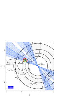
Figure 1: Left: constraints in the $(\bar{\rho},\bar{\eta})$ plane where $\bar{\rho}$ and $\bar{\eta}$ are defined by $\bar{\rho}=\rho(1-\lambda^{2}/2)$, $\bar{\eta}=\eta(1-\lambda^{2}/2)$. Shown are the $5~{}\%$ CLs for the individual constraints as shaded areas and the $1\sigma$- and $2\sigma$- contours from $\sin{2\beta}$. In addition, the $5~{}\%$ and $90~{}\%$ CL contours for the combined fit are drawn. Right: constraints in the $(\bar{\rho},\bar{\eta})$ plane if the likelihood ratio is used for the $\Delta m_{s}$ constraint.

The input values used in this analysis are listed in Tab. 1. For $|V_{ub}|$, inclusive measurements from LEP and exclusive measurements from CLEO have been used. The preliminary CLEO lepton endpoint analysis CLEOsemileptonic using moments obtained from $B\rightarrow X_{s}\gamma$ is not yet included. For $|V_{cb}|$, inclusive measurements from LEP, the measurements of $B\rightarrow D^{*}\ell\nu$ at zero-recoil and the moments analysis from CLEO CLEOsemileptonic , using inclusive $B\rightarrow X_{c}\ell\nu$ and $B\rightarrow X_{s}\gamma$ decays, have been combined. The uncertainty on $\Delta m_{d}$ has been significantly reduced due to the measurements from the $B$-factories sin2beta . However, the constraint on ($\bar{\rho},\bar{\eta}$) is not improved since it is dominated by the theoretical uncertainty on $f_{B_{d}}\sqrt{B_{d}}$. For $\Delta m_{s}$, the most recent combined amplitude spectrum from LEPB is included in the fit using a modified version of the standard amplitude method HLLL . If the amplitude spectrum is translated into a likelihood ratio RoussarieMoser ; Ciuchini , a stronger constraint is obtained. However, to our knowledge, it has not been demonstrated so far that the likelihood ratio can be interpreted as a probability density function. Hence, we use the more conservative method of Ref. HLLL for the numerical analysis presented here. For $\sin\!{2\beta}$, the world average is used. It should be noted that the most precise measurements from BABAR and Belle sin2beta differ presently by about two standard deviations.

2 Fit Results

The global minimum of the CKM fit is found to be $\chi^{2}_{{\rm min};y_{\rm mod}}=2.3$, resulting in a goodness-of-fit of $71\%$. It quantifies the excellent agreement between experimental data and the CKM picture of the SM. Fig. 1 shows the $(\bar{\rho},\bar{\eta})$ plane. Drawn are $5\%$ CL contours from the single constraints using $\Delta m_{d}$, $\Delta m_{s}$, $|V_{ub}/V_{cb}|$ and $|\epsilon_{K}|$, respectively, and the $1\sigma$- and $2\sigma$-contours for the four-fold ambiguity on $\beta$ from $\sin{2\beta}$. Shown in addition are the contours for the combined fit including $\sin\!{2\beta}$. The statistical precision of the $\sin\!{2\beta}$ measurement already competes with the indirect, theoretically limited constraints. Fig. 1 (right) illustrates the improved constraint when using the likelihood ratio for $\Delta m_{s}$. Selected numerical results are summarized in Tab. 1.

3 Charmless Two Body Decays

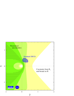
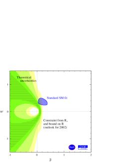
Figure 2: Left: Constraints in the $(\bar{\rho},\bar{\eta})$ plane using $R_{*}$ (see text) and the bound on $R$. The CL is indicated by the shaded areas; dark-grey: $>90~{}\%$, gray: $90~{}\%-32~{}\%$, light-gray: $32~{}\%-5~{}\%$. Right: Hypothetical constraints for summer 2002.

Constraints on the angle $\gamma$ can be obtained from $B\rightarrow\pi\pi,K\pi$ decays. Based on color transparency arguments, theoretical calculations such as the QCD Factorisation Approach (FA) BBNS and the QCD hard scattering approach KLS have been developed. Recently, the FA has been implemented in CKMfitter. At present, it is premature to infer reliable constraints on the basis of these calculations due to open theoretical questions BBNS ; KLS ; CFMPS . Data from the $B$-factories are not yet precise enough to probe the calculations in detail. Hence, all fit results are marked by an appropriate “${\rm R\&D}$” logo.
For this review, a global fit to $B\rightarrow\pi\pi,K\pi$ branching fractions and direct CP asymmetries measured in self-tagging $B\rightarrow K\pi$ decays has been performed within the framework of the FA, where most recent experimental results from BABAR BABAR , Belle BELLE and CLEO CLEO have been used. The numerous theoretical parameters are let free to vary within the ranges given in Ref. BBNS . We find $\chi^{2}_{{\rm min};y_{\rm mod}}=2.0$ and conclude that data are consistently described within the FA. The best FA fits are found at $\gamma\approx 80^{\circ}$ and are in agreement with the constraints from the standard fit.
Using less theoretical assumptions, ratios of branching fractions can be formed to derive constraints in the $(\bar{\rho},\bar{\eta})$ plane. As an example, the CP-averaged ratio

$$R=\frac{\tau_{B^{\pm}}}{\tau_{B^{0}}}\frac{{\cal B}(B^{0}\rightarrow K^{\pm}\pi^{\mp})}{{\cal B}(B^{\pm}\rightarrow K^{0}\pi^{\pm})}~{},$$ (1)

provides the bound $R>\sin^{2}\gamma$ which is independent of the strong phases FM . Unfortunately, the present world average $R=1.07^{+0.19}_{-0.15}$ leads to weak constraints only owing to the tails of the experimental errors. The ratio

$$R_{*}=\frac{{\cal B}(B^{\pm}\rightarrow K^{0}\pi^{\pm})}{2\cdot{\cal B}(B^{\pm}\rightarrow K^{\pm}\pi^{0})}~{},$$ (2)

measured to be $R_{*}=0.70^{+0.16}_{-0.13}$, can be used to derive bounds in the $(\bar{\rho},\bar{\eta})$ plane NR . An important input for the theoretical prediction of $R_{*}$ is the tree-to-penguin ratio (P/T) which can be determined experimentally using the relation

$$\bar{\epsilon}_{3/2}=R_{\rm th}\cdot\tan\theta_{\rm C}\cdot\frac{f_{K}}{f_{\pi}}\sqrt{\frac{2\cdot{\cal B}(B^{\pm}\rightarrow\pi^{\pm}\pi^{0})}{{\cal B}(B^{\pm}\rightarrow K^{0}\pi^{\pm})}~{},}$$ (3)

where $R_{\rm th}$ stands for SU(3) breaking corrections estimated in the FA to be BBNS $R_{\rm th}=0.98\pm 0.05$. The bound on $R_{*}$ can be translated into a prediction if additional information on the strong phases is inserted BBNS . Adopting the values for theoretical ranges quoted in Ref. BBNS , one obtains the constraints shown in Fig. 2. At present, the constraints remain rather weak due to the limited experimental precision. The slight deformation of the shape pattern around $\gamma\approx 90^{\circ}$ is due to the bound on $R$. For summer 2002, an integrated luminosity of $100~{}{\rm fb^{-1}}$ is expected to be collected by each experiment, BABAR and Belle. The experimental precision will then start to provide interesting constraints, as can be seen from Fig. 2 obtained assuming the present central experimental values and appropriately rescaling their errors. However, the constraints would still rely on the validity of some theoretical assumptions not yet fully explored.
Within the FA, the P/T ratio for $B\rightarrow\pi^{+}\pi^{-}$ is predicted. Compared to the present experimental error on the time-dependent asymmetry $S_{\pi\pi}=0.03^{+0.53}_{-0.56}\pm 0.11$ from BABAR, the quoted theoretical uncertainty is much smaller BBNS . In Fig. 3 (left), the constraints in $(\bar{\rho},\bar{\eta})$ from $S_{\pi\pi}$ are shown using P/T from FA where theoretical uncertainties have been neglected. The right plot shows the constraints when also using $\sin\!{2\beta}$.

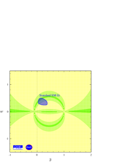
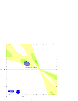
Figure 3: Left: Constraints on $(\bar{\rho},\bar{\eta})$ from $S_{\pi\pi}$ using the penguin-over-tree ratio from FA. Right: Constraints when using also $\sin\!{2\beta}$.

References

• (1) N. Cabibbo, Phys. Rev. Lett. 10, 531 (1963); M. Kobayashi and T. Maskawa, Prog. Th. Phys. 49, 652 (1973).
• (2) A. Höcker, H. Lacker, S. Laplace and F. Le Diberder, Eur. Phys. Jour. C21/2, 225 (2001).
• (3) “CKMfitter: code, numerical results and plots”, http://ckmfitter.in2p3.fr/.
• (4) L. Wolfenstein, Phys. Rev. Lett. 51, 1945 (1983).
• (5) R.A. Briere, these proceedings.
• (6) T. Browder and S. Prell, these proceedings.
• (7) LEP $B$ Oscillation WG, http://lepbosc.web.cern.ch/LEPBOSC/combined_results/budapest_2001/.
• (8) H.G. Moser and A. Roussarie, Nucl. Instr. Meth. A384, 491 (1997).
• (9) M. Ciuchini et al., Jour. High Ener. Phys. 0107, 013 (2001).
• (10) M. Beneke, G. Buchalla, M. Neubert and C.T. Sachrajda, hep-ph/0104110, (2001).
• (11) Y.-Y. Keum, H.-n. Li, and A.I. Sanda, hep-ph/0004173, (2000).
• (12) M. Ciuchini et al., hep-ph/0104126, (2001).
• (13) BABAR coll., hep-ex/0105061, (2001); hep-ex/0107074, (2001).
• (14) Belle coll., hep-ex/0104030 (2001); hep-ex/0106095, (2001).
• (15) CLEO coll., Phys. Rev. Lett. 85, 515 (2000); Phys. Rev. Lett. 85; 525 (2000).
• (16) R. Fleischer and T. Mannel, Phys. Rev. D57, 2752 (1998).
• (17) M. Neubert and J.R. Rosner, Phys. Lett. B441, 403 (1998).