Transverse Momentum Dependence of Intercept Parameter $\lambda$ of Two-Pion (-Kaon) Correlation Functions in q-Bose Gas Model

Abstract

Within recently proposed approach aimed to effectively describe the observed non-Bose type behavior of the intercept $\lambda$ of two-particle correlation function $C(p,K)$ of identical pions or kaons detected in heavy-ion collisions, the $q$-deformed oscillators and $q$-Bose gas picture are employed. For the intercept $\lambda$, connected with deformation parameter $q$, the model predicts a fully specified dependence of $\lambda$ on pair mean momentum ${\bf K}$. The intercepts $\lambda_{\pi}$ and $\lambda_{K}$ for pions and kaons, differing noticeably at small ${\bf K}$, should merge at ${\bf K}$ large enough, i.e., in the range $|{\bf K}|\ \geq\!800$ MeV/c, where the effect of resonance decays is negligible. In this paper we confront, fixing $q$ appropriately, the predicted dependence $\lambda_{\pi}=\lambda_{\pi}({\bf K})$ with recent results from STAR/RHIC for $\pi^{-}\pi^{-}$ and $\pi^{+}\pi^{+}$ pairs, and find nice agreement. Using the same $q$, we also predict behavior of $\lambda$ for kaons.

Two-particle correlations in momentum space can be used to extract information about the space-time structure of the emitting sources created in heavy ion collisions. The method exploits in an essential way the quantum mechanical uncertainty relation between coordinates and momenta, and thus any formal treatment of two-particle correlations must be based on a quantum mechanical description. For so-called ”chaotic” sources where the two particles are emitted independently the description can be based on the single-particle Wigner density $S(x,K)$ of the source (source function).

In standard quantum mechanical treatment the Bose-Einstein correlations are due to symmetrization of the two-particle (many-particle) wave function (suppose particles are emitted independently) $\psi_{\gamma_{a}\gamma_{b}}({\bf x}_{a},{\bf x}_{b},t)=\frac{1}{\sqrt{2}}\big{[}\psi_{\gamma_{a}}({\bf x}_{a},t)\,\psi_{\gamma_{b}}({\bf x}_{b},t)\,+\,e^{i\alpha}\psi_{\gamma_{a}}({\bf x}_{b},t)\,\psi_{\gamma_{b}}({\bf x}_{a},t)\big{]}$ with $\alpha=0$ ($\alpha=\pi$) for identical bosons (fermions). The indices $\gamma_{a},\gamma_{b}$ of the 1-particle wave functions label complete sets of 1-particle quantum numbers. In the following, we consider two-particle correlations of noninteracting spin zero identical bosons. The correlation function, with $P_{1}\left({\bf k}\right)$ and $P_{2}\left({\bf k}_{a},{\bf k}_{b}\right)$ being single- and two-particle probabilities to detect particles with given momenta, is defined as

$$C({\bf k}_{a},{\bf k}_{b})=\frac{\displaystyle P_{2}\left({\bf k}_{a},{\bf k}_{b}\right)}{\displaystyle P_{1}\left({\bf k}_{a}\right)\,P_{1}\left({\bf k}_{b}\right)}.$$

In the absence of final state interactions (FSI, see AHR ), for chaotic source, the correlation function can be expressed as follows AGI :

$$C({\bf k}_{a},{\bf k}_{b})=1\,+\,\cos{\alpha}\,\frac{\left|\int d^{4}x\,e^{ip\cdot x}S(x,K)\right|^{2}}{\int d^{4}x\,S\big{(}x,k_{a}\big{)}\,\int d^{4}y\,S\big{(}y,k_{b}\big{)}}$$ (1)

with the 4-momenta $K=\frac{1}{2}(k_{a}+k_{b})$ as pair mean momentum and $p=k_{a}-k_{b}$ as relative momentum. The source function $S(x,K)$ is defined by the single-particle states $\psi_{\gamma}(x)$ at freeze-out time and the source density matrix $\rho_{\gamma\gamma^{\prime}}$ as, e.g., in AGI . Obviously, from (1) at zero relative momentum ${\bf k}_{a}={\bf k}_{b}$ one gets $C({\bf k}_{a},{\bf k}_{a})=1+\cos\alpha\equiv 1+\lambda$ and since for bosons $\alpha=0$ it follows that $C({\bf k}_{a},{\bf k}_{a})=2$, i.e., $\lambda=1\,.$ To fit experimental data, the correlation function of identical bosons is usually presented as $C(p,K)=1\,+\,\lambda\,f(p,K)$, with $f(p,K)$ commonly taken as Gaussian so that $f({\bf p}=0,K)=1$. From the very first experiments it was deduced that $\lambda$ is lesser than one, the typical experimental values being $\lambda=$ 0.4 - 0.9 . The second term in (1) is obviously due to quantum-mechanical interference, and deviation of $\lambda$ from unity manifests weakening of the interference effects which can occur due to different reasons - influence of long lived resonances, coherent emission, etc.

Let us explain the key idea of the model developed in AGI ; AGI2 (named AGI-model in what follows) and further exploited in this letter. In two-boson correlations the deviation of intercept $\lambda$ from unity, besides the contribution due to effects from long-lived resonances, can also be caused by the averaged softening of quantum-statistical effects in the peculiar short-lived many-particle systems formed in relativistic heavy ion collisions. In such small system, the symmetrization angle $\alpha$ of $\psi_{\gamma_{a}\gamma_{b}}({\bf x}_{a},{\bf x}_{b},t)$ can be distorted by an additional phase due to a nonhomogenuity of the system at freeze-out times (strong radial and azimuthal flows). These peculiarities can cause the effect analogous to Aharonov-Bohm one. As result, a finite value of averaged symmetrization angle may appear: $\overline{\alpha}>0$ for bosons and $\overline{\alpha}<\pi$ for fermions.

Now, trying to explain experimental data with formula (1), it is natural to relate the parameter $\lambda$ with the averaged angle $\overline{\alpha}$ to get the reduction factor $\lambda$ by means of $\cos{\overline{\alpha}}$. That is, the deviation of intercept $\lambda$ from unity is viewed to be due to fluctuations of symmetrization angle $\alpha$, i.e.

$$\lambda=\cos{\overline{\alpha}}\,.$$ (2)

Notice that slow bosons (pions, kaons) will experience bigger fluctuations (deviations) of symmetrization angle $\alpha$ than the particles with high velocities in fireball frame. That is, the deviation of intercept $\lambda$ from unity for slow bosons should be more sizable than for the fast ones.

To implement our key idea we exploit quantum field theory with $q$-deformed commutation relations (qDCR) and the techniques of $q$-boson statistics (see VZ and refs. therein) which reflects a partial suppression of the quantum statistical effects. In tsallis94 ; arik99 it was argued that the algebra of qDCR is connected, for real $q$ only, with the so-called nonextensive statistics introduced by Tsallis tsallis88 . This type of generalized statistics has already found numerous applications in diverse branches of modern physics (see tsallis99 for refs.). In particular, nonextensive statistics was applied to the problems of high-energy nuclear collisions (UWW00 and refs. therein). However, the techniques of $q$-boson statistics based on qDCR allows the use of complex values as well as the real values for the deformation parameter $q$, depending on the choice of algebraic realization of qDCR. The physical reasons for usage of qDCR, and subsequent interpretation of $q$, essentially differ depending on the case of $q$ real or complex. Introducing deformed statistics with $q$ real enables one to effectively account for interaction effects by means of non-interacting ideal gas of “modified” particles. On the other hand, the approach based on qDCR provides the ability to model the effects involving the Aharonov-Bohm like phase, intimately connected with symmetrization properties of wave functions.

For the system of pions or kaons produced in heavy ion collisions, we employ the ideal $q$-Bose gas picture. Physical meaning or explanation of the origin of $q$-deformation in the considered phenomenon sharply differs in the case of real deformation parameter $q$ from the case when $q$ is a pure phase factor, as will be seen in what follows.

The AGI-model exploits two different sets of qDCR. The first is the multimode Biedenharn-Macfarlane (BM-type) $q$-oscillator defined as BM : $[N_{j},b_{j}]=-b_{j},\$ $[N_{j},b^{\dagger}_{j}]=b^{\dagger}_{j},\$ $b_{j}b_{j}^{\dagger}-q^{-1}b_{j}^{\dagger}b_{j}=q^{N_{j}},$ where different modes ($i\neq j$) commute. Then, $b^{\dagger}_{i}b_{i}=[N_{i}]_{q}$ (here the “$q$-bracket” means $[r]_{q}=(q^{r}-q^{-r})/(q-q^{-1})$ ) so that $b^{\dagger}_{i}b_{i}=N_{i}$ is recovered in the “classical” (“no deformation”) limit $q\to 1$ . Below, for the BM-type $q$-oscillators it is meant that

$$q=\exp(i\theta)\ ,\ \ \ \ \ \ \ \ \ \ 0\leq\theta<\pi/2\ .$$ (3)

The second multimode $q$-oscillator used in AGI-model is the set of Arik-Coon (AC-type) $q$-oscillators, defined by the relations AC $[{\cal N},a]=-a,$ $[{\cal N},a^{\dagger}]=a^{\dagger},$ and $aa^{\dagger}-qa^{\dagger}a=1$ (subscript suppressed). Again, at $q\!\neq\!1$, the bilinear $a^{\dagger}_{i}a_{i}$ does not equal the number operator ${\cal N}_{i}$ (as is true for usual bosonic oscillators, i.e., at $q=1$). Instead, $a^{\dagger}_{i}a_{i}=[[{\cal N}_{i}]]$ where now the notation $[[r]]\equiv(1-q^{r})(1-q),$ is used. The $q$-bracket $[[\hat{A}]]$ for an operator $A$ is understood as a formal series. At $q\to 1$, from $[[\hat{A}]]$ one recovers $\hat{A}$. In what follows we set

$$-1\leq q\leq 1\ .$$ (4)

For each such value of the deformation parameter $q$, the $a^{\dagger}_{i}\$ and $\ a_{i}$ are mutual conjugates. Note that the inverse of the relation $a^{\dagger}_{i}a_{i}=[[{\cal N}_{i}]]$ is given by a formula expressing the operator ${\cal N}_{i}$ as a formal series of creation/annihilation operators.

For a multi-pion (-kaon) system, viewed as ideal gas of $q$-bosons the Hamiltonian is taken as

$$H=\sum_{i}{\omega_{i}{N}_{i}}$$ (5)

with $i$ labelling energy eigenvalues, $\omega_{i}=\sqrt{m^{2}+{\bf k}_{i}^{2}}$, and $N_{i}$ defined as above. This is unique truly noninteracting Hamiltonian with additive spectrum VZ . We assume discrete $3$-momenta of particles (the system is in a box of volume $\sim L^{3}$). For the set of AC-type $q$-oscillators, one takes ${\cal N}_{i}$ instead of $N_{i}$ in (5).

Statistical properties are obtained by evaluating thermal averages $\langle A\rangle={\rm Sp}(A\rho)/{\rm Sp}(\rho)\$, $\rho={\rm e}^{-\beta H}$ , with the Hamiltonian (5) and $\beta=1/T$.

With $b^{\dagger}_{i}b_{i}=[N_{i}]_{q}$ and $q+q^{-1}=[2]_{q}=2\cos\theta$, the $q$-deformed distribution function is obtained as VZ ; AG ; AGI

$$\langle b_{i}^{\dagger}b_{i}\rangle=\frac{1}{{\rm e}^{\beta\omega_{i}}-1+\delta_{i}}\ ,\ \ \ \ \delta_{i}=2~{}\frac{1-\cos\theta}{\ 1-{\rm e}^{-\beta\omega_{i}}}\ .$$ (6)

If $\theta\to 0$, it yields Bose-Einstein (BE) distribution. Note that the $q$-distribution function (6) is real.

The $q$-distribution (6) deviates from the quantum Bose-Einstein just in the “right direction” towards the classical Boltzmann distribution, that reflects a decreasing of quantum statistical effects. For kaons, whose mass $m_{K}$ is bigger than $m_{\pi}$, analogous curve should lie closer, than pion’s one, to that of BE distribution AGI2 .

In the case of AC-type $q$-bosons with real $q$ from (3), one arrives at the distribution function (cf. VZ ; AG ; AGI ):

$$\langle a_{i}^{\dagger}a_{i}\rangle=\frac{1}{{\rm e}^{\beta\omega_{i}}-q}\ .$$ (7)

In the no-deformation limit $q\to 1$, this also reduces to the Bose-Einstein distribution, since at $q=1$ we return to the standard system of bosonic commutation relations.

The deviation from standard BE statistics is natural thing if one considers the system of interacting particles versus that of non-interacting particles (ideal gas). For instance, natural type of interaction is the hard-core repulsion of the particles that assumes particle finite self-volume. This type of interaction, as was shown in anch92 , results in the same kind (6) of modified statistics. At microscopical level, a finite self-volume arising due to composite structure of particles results in $q$-deformed commutation relations avancini95 and subsequently results in certain $q$-deformed statistics of the gas of such particles.

The two-particle distribution corresponding to the BM-type $q$-oscillators is

$$\langle b_{i}^{\dagger}b_{i}^{\dagger}b_{i}b_{i}\rangle=\frac{2\cos\theta}{{\rm e}^{2\beta\omega_{i}}-2\cos(2\theta){\rm e}^{\beta\omega_{i}}+1}\ .$$ (8)

From this and eq. (5), one obtains the intercept $\tilde{\lambda}_{i}\equiv\lambda_{i}+1=\langle b_{i}^{\dagger}b_{i}^{\dagger}b_{i}b_{i}\rangle/(\langle b_{i}^{\dagger}b_{i}\rangle)^{2}$ of two-particle correlations (subscript omitted) as

$$\lambda=-1+\frac{2\cos\theta\ (\cosh(\beta\omega)-\cos\theta)^{2}}{(\cosh(\beta\omega)-2\cos^{2}\theta+1)(\cosh(\beta\omega)-1)}.$$ (9)

At $\beta\omega\to\infty$ (i.e., at low temperature and fixed momenta or large momenta and fixed temperature) the asymptotics of intercept is given merely by the deformation angle $\theta$ (recall that $q=\exp({\rm i}\theta)$):

$$\lambda=\lambda^{\rm asymp}=2\cos\theta-1\hskip 17.07164pt(T\to 0\ \ {\rm or}\ \ |{\bf K}|\to\infty).$$ (10)

From this and eq. (2) we have the (asymptotical) relation $\cos\theta=\cos^{2}\frac{\overline{\alpha}}{2}$. Note that, if the unique cause forcing the intercept to be lesser than one is the decays of resonances (the conventional viewpoint), all the curves would tend to the value $\lambda=1$ in the large $|{\bf K}|$ limit. In contrast, we predict a constant $\lambda<1$, as in (10).

In the case of AC-type $q$-oscillators, the formula $\langle a_{i}^{\dagger}a_{i}^{\dagger}a_{i}a_{i}\rangle=({1+q}){({\rm e}^{\beta\omega_{i}}-q)^{-1}({\rm e}^{\beta\omega_{i}}-q^{2})^{-1}}$ for two-particle distribution combined with (6) leads to

$${\lambda}=-1+\langle a^{\dagger}a^{\dagger}aa\rangle/\langle a^{\dagger}a\rangle^{2}=q-\frac{q~{}(1-q^{2})}{{\rm e}^{\beta\omega}-q^{2}}.$$ (11)

In this case, for $T\to 0\$ or $\ |{\bf K}|\to\infty$ we have ${\lambda}^{\rm asymp}=q$.

Below, the two versions (9) and (11) corresponding to BM- and AC-types of $q$-deformation are compared to the recent STAR/RHIC data. The experimental values for intercept parameter $\lambda$ in Figs. 1 and 2 are taken from Ref. star . The theoretical values are obtained by averaging over given rapidity y and transverse momentum $K_{t}$ intervals $\Delta_{j}\equiv K_{t}^{j,{\rm max}}-K_{t}^{j,{\rm min}}$, $j=1,2,3$:

$$\lambda_{j}=\frac{1}{\Delta_{y}}\int\limits_{-\Delta_{y}/2}^{\Delta_{y}/2}{\rm d}y\,\frac{1}{\Delta_{j}}\int\limits_{K_{t}^{j,{\rm min}}}^{K_{t}^{j,{\rm max}}}{\rm d}K_{t}~{}\lambda(q,m,T,y,K_{t}),$$ (12)

where $m$ is particle mass.

Expressions (11) and (9) for $\lambda(q,m,T,y,K_{t})$ were used in (12) for obtaining theoretical points shown in Fig. 1 and Fig. 2 respectively.

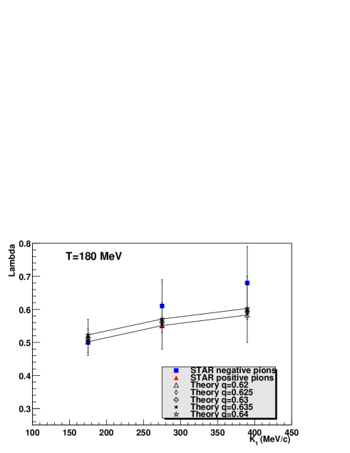
Figure 1: The transverse momentum $|{\bf K}_{t}|$ dependence of the intercept $\lambda$ of two-pion correlation. Deformation parameter $q$ is a real quantity, $0\leq q\leq 1$.

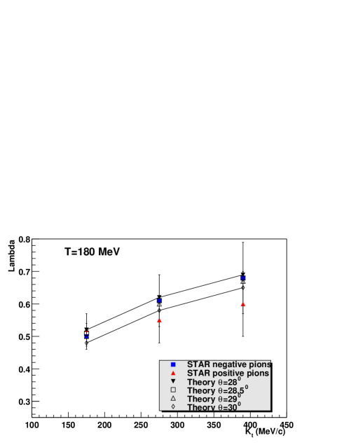
Figure 2: The transverse momentum $|{\bf K}_{t}|$ dependence of the intercept $\lambda$ of two-pion correlation. The deformation parameter $q$ is taken in the form $q=e^{i\theta}$.

One can see from these figures that the agreement of experimentally measured values of intercept parameter $\lambda$ with the theoretically calculated ones is very good.

Detailed comparison with the experiment star gives: the values $\lambda_{i}$ obtained from (13) at real $q$, see (12), fit better the three experimental values for the intercept of $\pi^{+}\pi^{+}$ correlations. On the other hand, the values calculated by (13) with $q$ a pure phase factor, see (10), agree better with the three experimental values for the intercept of $\pi^{-}\pi^{-}$ correlations. Possible explanation of the observed difference between experimental values of intercept for $\pi^{-}\pi^{-}$-pairs and $\pi^{+}\pi^{+}$-pairs could be the influence of the Coulomb FSI of these charged pions with the positive charge of fireball protons. Since the AGI-model predicts that parameter $\lambda$ will asymptotically reach a constant value $\lambda^{\rm asymp.}<1$, determined by $q$ only, at sufficiently large ($500\!-\!600$ MeV/c) pion pair mean momentum $|{\bf K}|$, in order to check this prediction measurements at higher $K_{t}$ are necessary. Such measurements should be available in near future at RHIC.

For the prediction of intercept of kaons, we will use the values of $q$ which provide the best fit of experimental data for pions (see Figs. 1 and 2): $q=0.63$ or $\theta=28.5^{\circ}$, assuming a universality of the deformation parameter for description of excited hot hadronic matter. The result of averaging in rapidity $-0.5\leq y\leq 0.5$, given by first integral in (12), is shown in Fig. 3 as solid curve in each of the triples of curves. The other two curves in each triple correspond to fixed value of rapidity: $y=0$ (dotted curve) and $y=0.5$ (dashed curve). Note that $y=0$ curve and solid curve almost coincide.

Figure 3: The transverse momentum $|{\bf K}_{t}|$ dependence of the intercept $\lambda$ of two-kaon correlation. Both the case of real $q=0.63$ (lower triple of curves) and the case of $q=e^{i\theta}$ (upper triple of curves) with $\theta=28.5^{\circ}$ are shown.

As it is clearly seen, the cases of real $q$ and $q$ a phase factor supply significantly different values for the kaon intercept $\lambda_{K}$. It is tempting to use just this feature for making preference of particular version of the deformation parameter $q$ - real or pure phase. The choice is important because differing physics is behind these two versions: real $q$ may reflect for instance particle finite size effects anch92 or particle composite structure avancini95 , and complex valued $q$ may refer to deformed symmetrization properties of wave functions (like in Aharonov-Bohm effect), relevant for short-lived systems occurred in heavy-ion collisions. It is also possible that a phase-type $q$ encodes gavr the effects from mixing at the composite (quark) level. Recent data from NA44 NA44 , i.e. $\lambda=0.84\pm 0.13$ and $\lambda=0.61\pm 0.36$ resp. for $\langle K_{t}\rangle\approx 0.25$ GeV/c and $\langle K_{t}\rangle\approx 0.91$ GeV/c do not yet help in making choice of optimal version for $q$.

In summary, we have presented comparison of the AGI model with experimental data on two-particle correlations at RHIC, and found remarkable agreement. We used the parameters extracted from comparison with pion’s data to predict behavior of intercept of kaon correlation functions. We stress again the crucial importance of correlation measurements at high transverse momenta in order to check the predicted asymptotical ”saturation” of intercept parameters. Measurements $|{\bf K}|$ in the range up to $500\!-\!600$ MeV/c for pions (up to $700\!-\!800$ MeV/c for kaons) should be possible by RHIC detectors such as STAR and PHENIX. The asymptotical behavior of intercept parameter $\lambda$ within the proposed model, see (10) for phase-type $q$, should determine the actual value of the deformation parameter $q$ supposed to be a universal quantity for relativistic heavy ion collisions.

D.A. acknowledges stimulating discussions with U. Heinz, valuable advices from P. Braun-Munzinger and expresses his gratitude to L. McLerran and Nuclear Theory Group (BNL) for fruitful discussions and warm hospitality. The work of A.G. was partially supported by the Award No. UP1-2115 of the U.S. Civilian Research and Development Foundation (CRDF).

References

- (1) D.V. Anchishkin, U. Heinz, and P. Renk Phys. Rev. C 57 1428 (1998) [nucl-th/9710051].
- (2) D.V. Anchishkin, A.M. Gavrilik and N.Z Iorgov, Europ. Phys. Journ. A 7 229 (2000) [nucl-th/9906034].
- (3) D.V. Anchishkin, A.M. Gavrilik and N.Z Iorgov, Mod. Phys. Lett. A 15 1637 (2000) [hep-ph/0010019].
- (4) S. Vokos and C. Zachos, Mod. Phys. Lett. A 9 1 (1994).
- (5) C. Tsallis, Phys. Lett. A 195 329 (1994).
- (6) M. Arik, Tr. J. of Physics 23 1 (1999).
- (7) C. Tsallis, J. Stat. Phys. 52 479 (1988).
- (8) C. Tsallis, Braz. J. Phys. 29 No.1 (1999).
- (9) O.V. Utyuzh, G. Wilk, Z. Wlodarczyk, J. Phys. G 26 L39 (2000). W.M. Alberico, A. Lavagno and P. Quarati, Eur. Phys. J. C 12 499 (2000).
- (10) A.J. Macfarlane, J. Phys. A 22 4581 (1989). L. Biedenharn, J. Phys. A 22 L873 (1989).
- (11) M. Arik and D.D. Coon, J. Math. Phys. 17 524 (1976). M. Arik, Z. Phys. C 51 627 (1991). D. Fairlie and C. Zachos, Phys. Lett. B 256 43 (1991). S. Meljanac and A. Perica, Mod. Phys. Lett. A 9 3293 (1994).
- (12) T.Altherr and T.Grandou, Nucl. Phys. B402 195 (1993). M.Daoud and M.Kibler, Phys. Lett. A 206 13 (1995).
- (13) D.V Anchishkin, Sov. Phys. JETP 75(2) 195 (1992).
- (14) S.S. Avancini, G. Krein, J. Phys. A 28 685 (1995).
- (15) C. Adler et al, The STAR Collaboration, Phys. Rev. Lett. 87 082301 (2001).
- (16) A.M. Gavrilik, in Proc. NATO ARW “Noncommutative Structures in Mathematics and Physics” (S. Duplij and J. Wess, eds.), Kluwer, 2001, p.343 [hep-ph/0011057].
- (17) NA44 Collaboration, I.G. Bearden et al., Phys. Rev. Lett. 87 112301 (2001).