The Entropy of the Quark-Gluon Plasma

Abstract

The entropy of the quark-gluon plasma can be calculated from QCD using (approximately) self-consistent approximations. Lattice results for pure gauge theories are accurately reproduced down to temperatures of the order of 2.5$T_{c}$. Comparisons with other approaches to the thermodynamics of the quark-gluon plasma are briefly discussed.

1 Introduction

As we were reminded, the Bielefeld meetings which took place in 1980 and 1982 have played a decisive role in our field. It should be added that, since then, the Bielefeld group has played a leading role in the study of QCD thermodynamics with lattice calculations. There is one particular result of that time that I wish to recall here because it is central to the topic of my talk. This result is that of the lattice calculation of the energy density of SU(2) pure gauge theory [1]. It is reproduced in Fig. 1 where one sees clearly the phase transition and the approach to the ideal gas limit at high temperature confirming expectations based on asymptotic freedom.

Modern results for the SU(3) equation of state [2] are displayed in Fig. 2. The talk will focus on the slow approach to the free gas limit of the thermodynamical functions at high $T$. The question that I wish to address is whether one can understand the deviation from the ideal gas behaviour with weak coupling calculations. Beyond this question is, as we shall see, another one related to the relevance of the notion of quasiparticles in the description of the quark-gluon plasma.

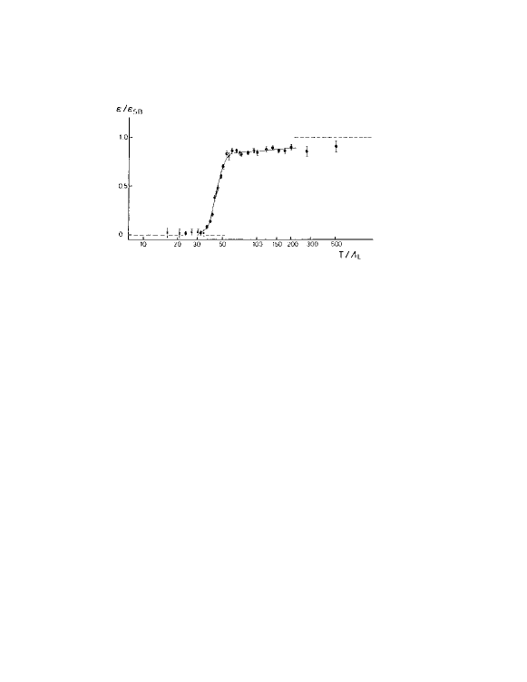
Figure 1: Energy density of a SU(2) gluon plasma normalized to that of an ideal gas of gluons, as a function of the temperature. From Ref. [1].

The motivation for considering the quark-gluon plasma as a weakly coupled system is of course asymptotic freedom, which leads us to expect that the effective coupling $g$ to be used in thermodynamical calculations should be small if the temperature $T$ is high enough:

$$\alpha_{s}(\mu)\,\equiv\,{g^{2}\over 4\pi}\,\propto\,\frac{1}{\ln(\mu/\Lambda_{QCD})}\,,$$ (1)

with typically $\mu\,\simeq\,2\pi T$. But we know that, even in cases where the coupling is small, strict perturbation theory cannot be used. Technically, infrared divergences occur in high order calculations, and various resummations are needed to get meaningful results.

Some of the difficulties of perturbation theory are already visible on the lowest orders which, for SU(3) gluons, read:

$$\frac{P}{P_{0}}=1-\frac{15}{4}\left(\frac{\alpha_{s}}{\pi}\right)+30\left(\frac{\alpha_{s}}{\pi}\right)^{3/2},$$ (2)

with $P_{0}$ the ideal gas pressure:

$$\qquad P_{0}=8\,\frac{\pi^{2}T^{4}}{45}.$$ (3)

The large coefficient of the $g^{3}$ term makes its contribution to the pressure comparable to that of the order $g^{2}$ when $g\mathrel{\hbox to0.0pt{\raise 2.20013pt\hbox{$>$}\hss}{\lower 2.20013pt\hbox{$\sim$}}}0.8$, or $\alpha_{s}\mathrel{\hbox to0.0pt{\raise 2.20013pt\hbox{$>$}\hss}{\lower 2.20013pt\hbox{$\sim$}}}0.05$; larger coupling makes the pressure larger than that of the ideal gas. Now it is worth emphasizing that the term of order $g^{3}$ emerges from an infinite resummation (strict perturbation theory at finite order would lead to a polynomial in $g^{2}$); it is the leading term of the resummed expression when $g$ is small. We shall later argue that the underlying strategy (that of performing an infinite resummation which is then re-expanded in powers of $g$) may not be used to extrapolate to large coupling. Physically the need for resummation arises from the existence of collective excitations in the system, whose properties are not well captured by perturbation theory.

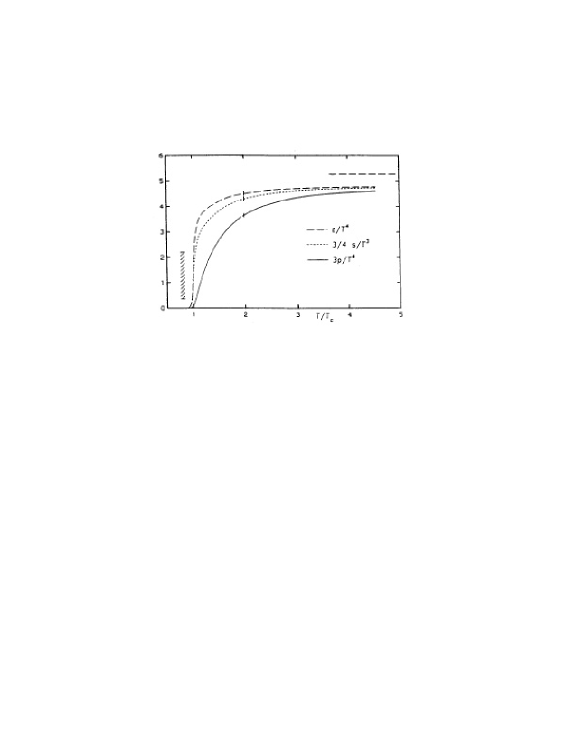
Figure 2: The thermodynamical functions in SU(3) gauge theories. From Ref. [2].

A lot of efforts have been devoted in the recent years to push perturbative calculations of the pressure to the highest calculable order, namely order $g^{5}$ [3, 4, 5]. The contributions of order $g^{4}$ and $g^{5}$ do not resolve the difficulties met at order $g^{3}$: the values of the pressure obtained by adding successively these high order contributions oscillate wildly, and reveal a strong dependence on the renormalization scale. Attempts have been made to construct smooth extrapolations based on the first terms of the series, using Pade approximants [6, 7] or Borel summation techniques [8, 9]. The resulting expressions are indeed smooth functions of the coupling, better behaved than polynomial approximations truncated at order $g^{5}$ or lower, with a weak dependence on the renormalization scale. However these techniques, which can be powerful, offer little physical insight.

A more appealing physical picture is provided by quasiparticle models in which one assumes that the dominant effect of the interactions can be incorporated in the spectral properties of suitably defined quasiparticles. It is useful to review briefly the simplest version of such models, limiting ourselves here to bosonic quasiparticles [10]. One assumes that the system is composed of non interacting massive quasiparticles with energies $E_{k}$:

$$E_{k}^{2}=k^{2}+m^{2}(T)$$ (4)

with the mass $m$ some function of the temperature. The entropy density is that of the ideal gas:

$$s=\int\frac{d^{3}k}{(2\pi)^{3}}\left[(1+N_{k})\log(1+N_{k})-N_{k}\log N_{k}\right],$$

where

$$\qquad N_{k}=\frac{1}{{\rm e}^{E_{k}/T}-1}.$$ (6)

The pressure $P$ and the energy density $\epsilon$ are then given by the corresponding ideal gas expressions, to within a function $B(T)$ adjusted so as to satisfy thermodynamical identities. That is, one sets:

$$P=-T\int\frac{d^{3}k}{(2\pi)^{3}}\log\left(1-{\rm e}^{-E_{k}/T}\right)-B(T)$$ (7)

$$\epsilon=\int\frac{d^{3}k}{(2\pi)^{3}}N_{k}E_{k}+B(T).$$ (8)

Such a parametrization obviously fulfills the identity $\epsilon+P=Ts$. The function $B(T)$ is then determined by requiring that

$$s=\frac{dP}{dT}.$$ (9)

Such a model has been shown to provide a quite good basis for a fit to lattice results [11]. Recent extensions of the model can be found in Ref. [12].

Finding a microscopic justification for this quasiparticle picture is the main motivation of the work that I shall present, summarizing results obtained in collaboration with E. Iancu and A. Rebhan [13, 14, 15, 16]. Our analysis is based on the entropy, for which the simple formulae above already suggest why it is simpler than the other thermodynamical functions: in both the pressure and the energy density there are interaction contributions, which cancel out in the entropy, leaving an expression in which all interaction effects are summarized in the properties of quasiparticles (in the simple model, the temperature dependent mass $m(T)$). We shall see later under which conditions this simple picture is valid.

At this stage, it is useful to have a more general characterization of the effects of weak interactions in a quark-gluon plasma. Let me then go through a short digression about the basic scales and degrees of freedom of such a system when the coupling is small [17].

2 Scales and degrees of freedom. Hard thermal loops

In the absence of interactions, the quark-gluon plasma is a gas of massless particles with energy $E_{k}=k$. Small interactions have little effects on most particles which have momentum $k\sim T$, but they strongly modify the propagation of low momentum modes. Since the coupling to gauge fields occurs typically through covariant derivatives, $D_{x}=\partial_{x}+igA(x)$, the effect of interactions on particle motion depends indeed on the momentum of the excitation and the magnitude of the gauge field. A measure of the strength of the gauge fields is obtained from the magnitude of their thermal fluctuations, that is $\bar{A}\equiv\sqrt{\langle A^{2}(t,{\bf x})\rangle}$. In equilibrium $\langle A^{2}(t,{\bf x})\rangle$ is independent of $t$ and ${\bf x}$ and given, in the non interacting case, by:

$$\langle A^{2}\rangle\approx\int\frac{{\rm d}^{3}k}{(2\pi)^{3}}\frac{N_{k}}{E_{k}}.$$ (10)

Here we shall use this formula also in the interacting case, assuming that the effects of the interactions can be accounted for simply by a change of $E_{k}$ (a more complete calculation is presented in Ref. [17]).

For the plasma particles $E_{k}=k\sim T$ and $\langle A^{2}\rangle_{T}\sim T^{2}$. The associated electric (or magnetic) field fluctuations $\langle(\partial A)^{2}\rangle_{T}\sim T^{4}$ are a dominant contribution to the plasma energy density. As already mentioned, these short wavelength, or hard, gauge field fluctuations produce a small perturbation on the motion of a plasma particle with momentum $k\sim T$, since $g\bar{A}_{T}\sim gT\ll k$. However, this is not so for an excitation at the momentum scale $k\sim gT$, since then the two terms in the covariant derivative $\partial_{x}$ and $g\bar{A}_{T}$ become comparable. That is, an excitation with momentum $gT$ is non perturbatively affected by the hard thermal fluctuations. And indeed, the scale $gT$ is that at which collective phenomena develop. The emergence of the Debye screening mass $m_{D}\sim gT$ is one of the simplest examples of such phenomena.

The fluctuations at the soft scale $gT\ll T$ can be described by classical fields. In fact the associated occupation numbers $N_{k}$ are large, and accordingly one can replace $N_{k}$ by $T/E_{k}\sim 1/g$ in eq. (10). Introducing an upper cut-off $gT$ in the momentum integral, one then gets:

$$\langle A^{2}\rangle_{gT}\sim\int^{gT}{\rm d}^{3}k\,\frac{T}{k^{2}}\sim gT^{2}.$$ (11)

Thus $\bar{A}_{gT}\sim\sqrt{g}T$ so that $g\bar{A}_{gT}\sim g^{3/2}T$ is still of higher order than the kinetic term $\partial_{x}\sim gT$. In that sense the soft modes with $k\sim gT$ are still perturbative, i.e. their self-interactions can be ignored in a first approximation. Note however that they generate contributions to physical observables which are not analytic in $g^{2}$, as shown by the example of the order $g^{3}$ contribution to the pressure (or as in eq.(11) above).

At the lower momentum scale $k\sim g^{2}T$, unscreened magnetic fluctuations play a dominant role. The contributions of such ultrasoft fluctuations is

$$\langle A^{2}\rangle_{g^{2}T}\sim T\int_{0}^{g^{2}T}{\rm d}^{3}k\frac{1}{k^{2}}\,\sim\,g^{2}T^{2},$$ (12)

so that $g\bar{A}_{g^{2}T}\sim g^{2}T$ is now of the same order as the ultrasoft derivative $\partial_{x}\sim g^{2}T$: the fluctuations are no longer perturbative. This is the origin of the breakdown of perturbation theory in high temperature QCD. A more detailed analysis reveals that the fluctuations at scale $g^{2}T$ come from the zero Matsubara frequency and correspond therefore to those of a three dimensional theory of static fields.

Having identified these various scales, we note now that the thermodynamical functions at high temperature are dominated by hard degrees of freedom. The quasiparticle picture that we shall develop takes into account consistently the contributions of the hard degrees of freedom together with those of the long wavelength collective excitations. We shall comment later on the techniques based on dimensional reduction which allows a treatment of the ultrasoft contributions.

There exists a well developed effective theory for the soft collective excitations that we briefly outline now. These soft excitations can be described in terms of average fields which obey classical equations of motion. In QED these equations are Maxwell equations:

$$\partial_{\mu}F^{\mu\nu}=j_{ind}^{\nu}+j_{ext}^{\nu}$$ (13)

with a source term composed of an external perturbation $j_{ext}^{\nu}$, and an extra contribution $j_{ind}^{\nu}$ referred to as the induced current. The induced current, which summarizes the effects of the hard degrees of freedom, can be obtained using linear response theory. It is of the form:

$$j_{\mu}^{ind}=\int{\rm d}^{4}y\,\Pi^{R}_{\mu\nu}(x-y)A^{\nu}(y),$$ (14)

where $A^{\nu}(y)$ is the total gauge field (including the induced potential) and the (retarded) response function $\Pi^{R}_{\mu\nu}(x-y)$ is also referred to as the polarization tensor. In leading order in weak coupling, this polarization tensor is given by the one-loop approximation, and can be written as $\Pi(\omega,p)=g^{2}T^{2}f(\omega/p,p/T)$ with $f$ a dimensionless function. Furthermore, the relevant kinematics is such that the incoming momentum is soft while the loop momentum is hard. Thus, in leading order in $p/T\sim g$, $\Pi$ is of the form $g^{2}T^{2}f(\omega/p)$. This particular contribution of the one-loop polarization tensor is an example of what has been called a “hard thermal loop” [18].

In a non Abelian theory, linear response is not sufficient: constraints due to gauge symmetry force us to take into account specific non linear effects. The relevant generalization of the Yang-Mills equation reads [19, 20] :

$$D_{\nu}F^{\nu\mu}=\Pi_{\mu\nu}^{ab}A_{b}^{\nu}+\frac{1}{2}\,\Gamma_{\mu\nu\rho}^{abc}A_{b}^{\nu}A_{c}^{\rho}+\,...$$ (15)

where the induced current in the right hand side is non-linear: when expanded in powers of $A^{\mu}_{a}$, it generates an infinite series of hard thermal loops (self-energy and vertex corrections).

In the next section, we shall consider various reorganizations of the perturbative expansion inspired by the previous analysis and which try to accommodate the non perturbative features associated with the various scales.

3 Reorganizing perturbative expansion

As we have seen, one of the main effects of the thermal fluctuations is to generate a mass for the soft modes. This is not peculiar to gauge theories, but occurs also in the simpler case of a scalar field. In this case, the mass generation can be taken into account non perturbatively by a very simple reorganization of the perturbative expansion, leading to the so-called “screened perturbation theory” [21]. One writes:

$${\cal L} = {\cal L}_{0}-\frac{1}{2}m^{2}\phi^{2}+\frac{1}{2}m^{2}\phi^{2}+{\cal L}_{int}$$ (16)

$$= {\cal L}_{0}^{\prime}+{\cal L}_{int}^{\prime}\,,$$

with ${\cal L}_{0}^{\prime}={\cal L}_{0}-(1/2)m^{2}\phi^{2}$. The mass $m\sim gT$ which appears here is for instance that obtained in leading order from the hard thermal loop. A perturbative expansion in terms of screened propagators (that is keeping the screening mass as a parameter, i.e. not as a perturbative correction to be expanded out) has been shown to be quite stable with good convergence properties. However, $m$ makes the propagators explicitly temperature dependent, and the ultraviolet divergences which occur in high order calculations become temperature dependent. Although we know that temperature dependent infinities should eventually cancel out, the systematics of such cancellations is not immediately transparent.

In the case of gauge theory, the effect of the interactions is more complicated than just generating a mass. But we know how to determine the dominant corrections to the self-energies. When the momenta are soft, these are given by the hard thermal loops discussed above. By adding these corrections to the tree level Lagrangian, and subtracting them from the interaction part, one generates the so-called hard thermal loop perturbation theory [22, 23, 24]:

$${\cal L}={\cal L}_{0}+{\cal L}_{HTL}-{\cal L}_{HTL}+{\cal L}_{int}={\cal L}_{0}^{\prime}+{\cal L}_{int}^{\prime}\,.$$ (17)

The resulting perturbative expansion is made complicated however by the non local nature of the hard thermal loop action, and by the necessity of introducing temperature dependent counter terms. Also, in such a scheme, one is led to use the hard thermal loop approximation in kinematical regimes where it is not justified.

Another approach that I wish to mention at this stage is that based on dimensional reduction. This approach puts emphasis on the non perturbative, very long wavelength fluctuations. It has been shown in Refs. [25, 26, 27] how, in principle, an effective theory could be constructed to deal with this particular problem by marrying analytical techniques (to determine the coefficients of the effective theory) and numerical ones (to solve the non perturbative 3-dimensional effective theory). The resulting effective theory is a 3-dimensional theory of static fields, with Lagrangian:

$${\cal L}_{eff}=\frac{1}{4}(F^{a}_{ij})^{2}+\frac{1}{2}(D_{i}A_{0}^{a})^{2}+\frac{1}{2}m_{D}^{2}(A_{0}^{a})^{2}+\lambda(A_{0}^{a})^{4}+\delta{\cal L},$$ (18)

with $D_{i}=\partial_{i}-ig\sqrt{T}A_{i}$. This strategy has been applied recently to the calculation of the free energy of the quark-gluon plasma a high temperature [28]. This technique of dimensional reduction puts a special weight on the static sector (it singles out the contributions of the zero Matsubara frequency), and a major effort is devoted to the calculation of the coefficients of the effective Lagrangian (which contain the dominant contribution to the thermodynamical functions).

In contrast, the approach that we have developed keep the full spectral information that one has about the plasma excitations. In a sense, it is close to the approach based on hard thermal loop perturbation theory. It differs in that we focus on the simplest of the thermodynamical function, namely the entropy, for which indeed interesting cancellations occur which allow us to bypass some of the difficulties of hard thermal loop perturbation theory.

4 Propagator renormalisation. Skeleton expansion

As already stated, we want to incorporate full spectral information about quasiparticles in thermodynamical calculations, and we are therefore led to carry out a propagator renormalisation. Although in gauge theory vertex renormalisation should be carried along with propagator renormalisation, we shall see here that special kinematical conditions allow us to develop useful approximations without having to do so.

The formalism that we shall rely on was developed long ago in the context of the non relativistic many-body problem. It is based on an expression for the pressure as a functional of full propagators, first written out by Luttinger and Ward [29]. Systematic developments using either functional Legendre transforms or diagrammatic formalisms were presented later by De Dominicis and Martin [30]. In implementing these methods to field theory one meets extra difficulties related to ultraviolet divergences. I now briefly outline the general method, writing explicitly only formulae appropriate for a scalar field (similar ones hold for QCD).

The free energy ${\cal F}$ can be written as the following functional of the full propagator $D$:

$${\cal F}[D]=\frac{1}{2}{\rm Tr}\ln D^{-1}-\frac{1}{2}{\rm Tr}\Pi D+\Phi[D],$$ (19)

where $\Phi$ is the sum of all the two-particle irreducible (skeletons) diagrams. The self-energy $\Pi$ is related to the propagator by Dyson’s equation

$$\,D^{-1}\,=\,D^{-1}_{0}\,+\,\Pi,$$ (20)

and $D_{0}$ is the bare propagator. A remarkable feature of the functional (19) is its stationarity property, i.e., ${\delta{\cal F}[D]/\delta D}\,=\,0$ when

$$\Pi[D]\,=\,2\frac{\delta\Phi}{\delta D}\,.$$ (21)

Together Eqs. (20) and (21) form a self-consistent set of equations which determine the full propagator. A major observation by Baym is that self-consistent approximations can be defined for any selection of skeleton diagrams in $\Phi$; furthermore such “$\Phi$-derivable” approximations have the property to respect the (global) symmetries of the hamiltonian [31].

The stationarity property of the free energy entails important simplifications in the calculation of the entropy. Indeed we have

$${\cal S}\,=\,-\,{{\rm d}{\cal F}\over{\rm d}T}\,=\,-\,{{\partial}{\cal F}\over{\partial T}}\bigg{|}_{D}$$ (22)

where the last step uses the fact that the temperature dependence of the propagator can be ignored. Explicitly one gets:

$${\cal S}=-\int\!\!\frac{d^{4}k}{(2\pi)^{4}}\frac{\partial N(\omega)}{\partial T}{\rm Im}\log D^{-1}(\omega,k)+\int\!\!\frac{d^{4}k}{(2\pi)^{4}}\frac{\partial N(\omega)}{\partial T}{\rm Im}\Pi(\omega,k){\rm Re}D(\omega,k)+{\cal S}^{\prime}$$ (23)

where $N(\omega)=1/({\rm e}^{\beta\omega}-1)$, and

$${\cal S}^{\prime}\equiv-\frac{\partial(T\Phi)}{\partial T}\Big{|}_{D}+\int\!\!\frac{d^{4}k}{(2\pi)^{4}}\frac{\partial N(\omega)}{\partial T}{\rm Re}\Pi\,{\rm Im}D.$$

A further simplification occurs when one restricts the choice of skeletons to low order ones [32, 33, 34]. Thus, for the two-loop skeletons in QCD, ${\cal S}^{\prime}=0.$

5 The 2-loop entropy

At two loop in the skeleton expansion, the entropy takes then the simple form [34, 13, 14, 15]:

$$S\,=\,-\int\frac{{\rm d}^{4}p}{(2\pi)^{4}}\,\frac{\partial N}{\partial T}\,\left\{{\rm Im}\ln D^{-1}\,-\,{\rm Im}\Pi\,{\rm Re}D\right\}$$ (24)

The simplifications discussed above have led to important cancellations leaving for the entropy an expression which is effectively a one-loop expression, thus emphasizing the direct relation between the entropy and the quasiparticle spectrum. Residual interactions start contributing at order 3-loop. This expression is also manifestly ultraviolet-finite.

Albeit simple, the 2-loop expression for the entropy is nevertheless difficult to use as it stands. Recall that the propagator and self-energy in this equation are solution of a self-consistent equation which is in general difficult to renormalize and to solve. Besides, in the case of gauge theories, the scheme does not fully respect gauge symmetry. We have therefore looked for additional approximations which exploits the simplicity of the scheme (the one-loop feature of the entropy formula) and at the same time allows for practical calculations. The main idea is to find gauge invariant approximations for the self-energy by exploiting kinematical approximations such as those which lead in particular to the hard thermal loops. The entropy is then calculated exactly with no further approximation. One constraint that we impose on our approximate $\Pi$ is that, once inserted in the formula (24), the resulting value of $S$ is perturbatively correct up to order $g^{3}$ (which is the maximum perturbative accuracy that one can achieve with 2-loop skeletons).

In the regime where the loop momenta are soft, we can use as an approximation for $\Pi$ the corresponding hard thermal loop (HTL), that is

$$\omega,\,p\sim gT\qquad\Pi_{soft}\,\approx\,\Pi_{HTL}$$

For hard momenta on the other hand, the hard thermal loop is no longer valid: corrections to hard particle dispersion relations due to their coupling with soft modes need to be taken into account. This can be estimated using usual HTL perturbation theory. A simplification occurs however because we need such corrections only near the light cone:

$$\omega,\,p\sim T\qquad\Pi_{hard}(\omega^{2}\sim p^{2})$$

In fact we shall find convenient to define two successive approximations. In the first one, called the HTL approximation, we use $\Pi=\Pi_{HTL}$ at all momenta. This is a fine approximation for soft momenta, but it is also a decent approximation at hard momenta because the self-energy is needed only in the vicinity of the light cone where the hard thermal loop approximation coincides with the full one-loop result. We call ${\cal S}_{HTL}$ the resulting expression for the entropy. This expression fully accounts for the perturbative contributions of order $g^{2}$ but for only $1/4$ of that of order $g^{3}$. In the next-to-leading approximation one uses $\Pi_{soft}=\Pi_{HTL}$ and $\Pi_{hard}=\Pi_{HTL}+\delta\Pi$, where $\delta\Pi$ contains the coupling to the soft modes (I should emphasize at this point that the construction of our next-to-leading approximation involves several subtle steps which I am skipping here but which are detailed by A. Rebhan in his contribution [16]). We call ${\cal S}_{NLA}$ the corresponding entropy; it takes fully into account all perturbative contributions of order $g^{2}$ and $g^{3}$.

As an illustration of the quality of the results which we can obtain, I present in Fig. 3 the entropy of pure SU(3) gauge theory normalized to the ideal gas entropy. The agreement at large $T$ ($T\mathrel{\hbox to0.0pt{\raise 2.20013pt\hbox{$>$}\hss}{\lower 2.20013pt\hbox{$\sim$}}}2.5T_{c}$) is quite good. Note also that in going from one level of approximation to the next (i.e. from ${\cal S}_{HTL}$ to ${\cal S}_{NLA}$), the changes are moderate, in contrast to what happens in ordinary perturbation theory. This reflects the stability of the present scheme. It also points to the fact that the contribution of the soft collective modes is indeed small: the fact that they give a seemingly large contribution at order $g^{3}$ in perturbation theory is just an artifact of the truncation of a resummed expression at finite order.

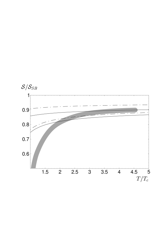
Figure 3: The entropy of pure SU(3) gauge theory normalized to the ideal gas entropy ${\cal S}_{SB}$. Full lines: ${\cal S}_{HTL}$. Dashed-dotted lines: ${\cal S}_{NLA}$. For each approximation, the two lines correspond to the choices $\bar{\mu}=\pi T$ and $\bar{\mu}=4\pi T$ of the running coupling constant $\alpha_{s}(\bar{\mu})$ in the $\overline{{\rm MS}}$ renormalization scheme. The dark grey band represents the lattice results of Ref. [2].

6 CONCLUSIONS

Our results confirm that for temperatures larger than about 3$T_{c}$, the thermodynamical functions of the quark-gluon plasma, in particular its entropy, can indeed be interpreted as those of weakly interacting quasiparticles. The dominant effect of the interactions is to modify the spectrum of these quasiparticles. As the coupling grows the quasiparticle properties are non perturbatively renormalized but their mutual interactions remain weak.

Thermodynamic functions are dominated by hard degrees of freedom. While long range correlations may survive in the quark-gluon plasma at very large temperature, the present picture suggests that such correlations do not contribute much to the thermodynamics. We find explicitly that the soft contributions are indeed small. We argued in particular that the contribution of collective modes is artificially amplified when the coupling is not too small by truncating this contribution at order $g^{3}$.

The approach that we have developed relies on a hierarchy of scales that emerges when the coupling is small. It is an assumption that the structure identified at weak coupling survives when the coupling grows, e.g. as we lower the temperature. The fact that we find approximations where such an extrapolation works supports the validity of this assumption. But of course a complete check of the method can only be done by comparing with “exact” results, such as those provided by lattice techniques. Much can be learned also from detailed comparisons with the other approaches discussed earlier, namely hard thermal loop perturbation theory or dimensional reduction. There is finally much to do also within the present theory itself, to push for instance non perturbative renormalization techniques (interesting progress in this direction has been reported recently [35]; see also [36]).

Further tests involve the calculations of different observables. An example, advocated by Gavai [37] at this workshop, is that of quark susceptibilities. This is a calculation that we have recently taken up, with interesting results [38]. The calculation of quark susceptibilities represents a small incursion into the physics of finite chemical potentials which is of course readily available in our approach [16].

References

- [1] J. Engels, F. Karsch, H. Satz and I. Montvay, Nucl. Phys. B 205 (1982) 545.
- [2] G. Boyd, J. Engels, F. Karsch, E. Laermann, C. Legeland, M. Lütgemeier, B. Petersson, Nucl. Phys. B469 (1996) 419–444.
- [3] P. Arnold and C. Zhai, Phys. Rev. D 50, 7603 (1994), ibid. 51, 1906 (1995); C. Zhai and B. Kastening, ibid. 52, 7232 (1995).
- [4] E. Braaten and A. Nieto, Phys. Rev. D 53, 3421 (1996).
- [5] E. Braaten, these proceedings.
- [6] T. Hatsuda, Phys. Rev. D 56 (1997) 8111 [hep-ph/9708257].
- [7] S. Chiku and T. Hatsuda, Phys. Rev. D 58 (1998) 076001 [hep-ph/9803226].
- [8] R. R. Parwani, Yang-Mills theory,” Phys. Rev. D 63 (2001) 054014 [hep-ph/0010234].
- [9] R. R. Parwani, Phys. Rev. D 64 (2001) 025002 [hep-ph/0010294].
- [10] A. Peshier, B. Kämpfer, O. P. Pavlenko, and G. Soff, Phys. Rev. D 54, 2399 (1996); A. Peshier, hep-ph/9809379.
- [11] P. Levai, U. Heinz, Phys. Rev. C57 (1998) 1879.
- [12] R. A. Schneider and W. Weise, Phys. Rev. C 64 (2001) 055201 [arXiv:hep-ph/0105242].
- [13] J. P. Blaizot, E. Iancu, A. Rebhan, Phys. Rev. Lett. 83 (1999) 2906–2909.
- [14] J. P. Blaizot, E. Iancu, A. Rebhan, Phys. Lett. B470 (1999) 181–188.
- [15] J. P. Blaizot, E. Iancu, A. Rebhan, Phys. Rev. D63 (2001) 065003.
- [16] A. Rebhan, these proceedings.
- [17] J. P. Blaizot and E. Iancu, arXiv:hep-ph/0101103.
- [18] E. Braaten and R. D. Pisarski, Nucl. Phys. B337, 569 (1990); J. Frenkel and J. C. Taylor, Nucl. Phys. B334, 199 (1990).
- [19] J.-P. Blaizot and E. Iancu, Nucl. Phys. B390, 589 (1993); Phys. Rev. Lett. 70, 3376 (1993); Nucl. Phys. B417, 608 (1994).
- [20] J.-P. Blaizot, E. Iancu and J.-Y. Ollitrault, in Quark-Gluon Plasma II, edited by R.C. Hwa (World Scientific, Singapore, 1996).
- [21] F. Karsch, A. Patkós, P. Petreczky, Phys. Lett. B401 (1997) 69–73.
- [22] J. O. Andersen, E. Braaten, M. Strickland, Phys. Rev. D63 (2001) 105008.
- [23] J. O. Andersen, E. Braaten, M. Strickland, Phys. Rev. Lett. 83 (1999) 2139–2142.
- [24] J. O. Andersen, E. Braaten, M. Strickland, Phys. Rev. D61 (2000) 014017.
- [25] E. Braaten, Phys. Rev. Lett. 74 (1995) 2164 [hep-ph/9409434].
- [26] E. Braaten and A. Nieto, Phys. Rev. Lett. 76 (1996) 1417 [hep-ph/9508406].
- [27] E. Braaten and A. Nieto, Phys. Rev. D 53 (1996) 3421 [hep-ph/9510408].
- [28] K. Kajantie, M. Laine, K. Rummukainen and Y. Schroder, Phys. Rev. Lett. 86 (2001) 10 [hep-ph/0007109].
- [29] J. M. Luttinger, J. C. Ward, Phys. Rev. 118 (1960) 1417.
- [30] C. De Dominicis and P.C. Martin, J. Math. Phys. 5, 14, 31 (1964).
- [31] G. Baym, Phys. Rev. 127 (1962) 1391.
- [32] E. Riedel, Z. Phys. 210 (1968) 403–422.
- [33] G. M. Carneiro and C. J. Pethick, Phys. Rev. B 11, 1106 (1975).
- [34] B. Vanderheyden, G. Baym, J. Stat. Phys. 93 (1998) 843.
- [35] H. van Hees, J. Knoll, Renormalization in self-consistent approximations schemes at finite temperature. I: Theory, hep-ph/0107200 (2001).
- [36] E. Braaten, E. Petitgirard, Solution to the 3-loop -derivable approximation for massless scalar thermodynamics, hep-ph/0107118 (2001).
- [37] R. Gavai, these proceedings.
- [38] J. P. Blaizot, E. Iancu and A. Rebhan, arXiv:hep-ph/0110369.