We consider the Brownian motion of a $c\bar{c}$ pair produced in the very early satge of a quark-gluon plasma. The one-dimensional Langevin equation is solved formally to get purely mechanical properties at small and large times. Stochastically-averaged variances are examined to extract the time scales associated with swelling and ionization of the bound state. Simple numerical estimates of the time scales are compared with other mechanisms of $J/\psi$ suppression.

PACS number(s): 12.38.Mh, 05.10.Gg, 52.65.Ff, 05.20.Dd

1 Introduction

Charmonium i.e., $J/\psi$ suppression [1] continues to be one of the most hotly debated signatures of the production of a quark-gluon plasma in ultrarelativistic heavy ion collisions. Both the initial formation and subsequent survival probabilities of the $J/\psi$ are affected by several factors viz. scattering with hard partons [2], Debye colour screening [1], drag and diffusion arising from Brownian motion [3, 4], evolution of the plasma via hydrodynamic flow [5], etc. Although the theoretical time scales for gluonic dissociation vs colour screened break-up are well known [6] the time scales for the swelling/ionization of $J/\psi$ caused by Brownian movement are not yet understood satisfactorily, and the aim of the present paper is to focus attention on this aspect.

The classical $3$-dimensional Fokker-Planck equation for the distribution function of a single charmed quark propagating in a plasma was first studied by Svetitsky [3]. Assuming soft scattering with the partons he found the associated Boltzmann transport coefficients for drag and diffusion to be rather large but he ignored the force which binds the $c\bar{c}$ pair. Plotnik and Svetitsky [7] extended this philosophy to the case of two-particle Fokker-Planck dynamics in the presence of a colour singlet/octet potential between the pair. However, since no attempt was made by them to actually solve the resulting $13$ variable partial differential equation, hence no simple estimate was given for the time scales of the $c\bar{c}$ pair.

In the present work we adopt a different approach based on analyzing the one-dimensional Langevin equation for the stochastic trajectory of a $c\bar{c}$ pair initially bound by a screened Coulomb field. It is known since long ago [8] that the Langevin theory provides a valid description of classical Brownian movement of a test particle acted upon simultaneously by a driving interaction, frictional force, thermal agitation, and random noise. In Sec.2 below we write formal solutions to the underlying equations of motion and obtain compact expressions for the purely mechanical observables at small and large times. Stochastic averaging of the observables is done in Sec.3 so as to deduce statistical properties (viz. means, variances, time scales, etc.) of the system. Sec.4 gives simple, order-of-magnitude estimates of the relevant time scales and discusses the result vis-a-vis other mechanisms of $J/\psi$ suppression. Finally, Sec.5 examines critically the validity of our main assumptions and also mentions several additional complications which would have to be incorporated in future applications of the theory.

2 Purely Mechanical Observables

2A. Assumptions & notations

For a nonrelativistic $c\bar{c}$ pair propagating in a spatially homogeneous plasma the net external colour force due to the background is zero although the internal screened Coulomb potential (assumed to be colour singlet) survives. Working in the barycentric frame and adopting a one-dimensional view we can describe the motion of an effective single particle by defining

$$t={\mbox{\rm{time}}},\quad m={\mbox{\rm{reduced mass}}},\quad x={\mbox{\rm{position}}},\quad u=\dot{x}={\mbox{\rm{velocity}}},$$

$$V=V(x)={\mbox{\rm{binding potential}}},\quad f=f(x)=-\partial V/\partial x={\mbox{\rm{binding force}}},$$

$$\gamma={\mbox{\rm{coefficient of friction (per unit mass) assumed constant}}},$$

$$T={\mbox{\rm{ambient temperature of medium in energy units}}},$$

$$h=h(t)={\mbox{\rm{random force taken as a white Gaussian noise}}},$$

$$C=2m\gamma T={\mbox{\rm{strength of the noise autocorrelation function}}},$$

$$D=C/2m^{2}\gamma^{2}=T/m\gamma={\mbox{\rm{Einstein diffusion coefficient}}}$$ (2.1)

The space derivative $f^{\prime}$ and total time derivative $\dot{f}$ of the force are written as

$$f^{\prime}=\partial f/\partial x,\quad\dot{f}=df/dt=uf^{\prime}$$ (2.2)

Since the pair potential $V$ depends upon $|x|$ the symmetry relations

$$V(-x)=V(x),\quad f(-x)=-f(x)$$ (2.3)

hold as shown schematically in Fig.1

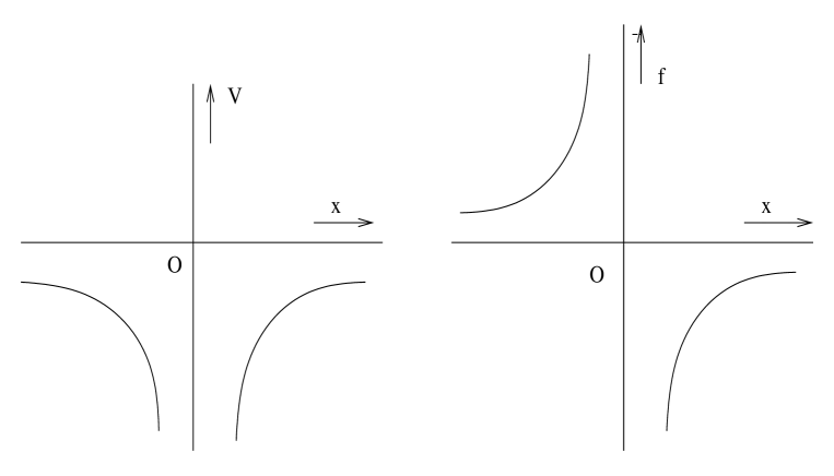
Figure 1: Schematic shapes of $c\bar{c}$ binding potential $V$ and force $f$.

Before proceeding further a few important comments are in order. One-dimensional stochastic models [8, 9] have been found very useful in the past because they are mathematically simple and can also simulate purely radial motion in three dimensions. The choice $C=2m\gamma T$ guarantees that the test particle’s distribution at asymptotic time would become Maxwell-Boltzmann at background temperature $T$ in accordance with the fluctuation-dissipation theorem [10]. Due to the same reason the single diffusion parameter $D=T/m\gamma$ gets fixed in terms of the temperature and the damping coefficient. All these remarks are, however, subject to alterations as will be pointed out later in Sec. 5.

2B. Langevin equation & the velocity

The basic ordinary differential equation to be considered is

$$\dot{u}+\gamma u=(f+h)/m,\quad\dot{x}=u$$ (2.4)

subject to the initial conditions

$$u(t=0)=u_{0},\quad x(t=0)=x_{0}$$ (2.5)

For a free particle and a harmonic oscillator, Eq.(2.4) was solved explicitly by Chandrasekhar [8] but the present case is more difficult because $f$ is a nonlinear function of $x$. Using the integrating factor $e^{\gamma t}$ we obtain a formal solution for the velocity as

$$u=u^{\mbox{\rm{fr}}}+v+w$$ (2.6)

Here the contributions arising from free Rayleigh motion, the driving force, and the random noise are respectively given by

$$u^{\mbox{\rm{fr}}} = u_{0}e^{-\gamma t},\quad v=\frac{e^{-\gamma t}}{m}\int_{0}^{t}dt_{1}e^{\gamma t_{1}}f_{1}$$

$$w = \frac{e^{-\gamma t}}{m}\int_{0}^{t}dt_{1}e^{\gamma t_{1}}h_{1}$$ (2.7)

with $t_{1}$ being an integration time and $f_{1}=f\mid_{t_{1}},\quad h_{1}=h\mid_{t_{1}}$.

At small times the driving force can be approximated by a first-order Taylor expansion

$$f_{1}\approx f_{0}+u_{0}f_{0}^{\prime}t_{1}+\cdot\cdot\cdot,\quad\quad\gamma t_{1}\ll 1$$ (2.8)

where the suffix $0$ refers to the instant when the $J/\psi$ was produced and the dots represent nonleading terms. Substituting into Eqs.(2.6), (2.7) we get the initial behaviour of the velocity and its square as

$$u \approx u_{0}+J_{0}t+\cdots+w\quad,\quad\quad t\ll\gamma^{-1}$$ (2.9)

$$u^{2} \approx \{u_{0}^{2}+2u_{0}J_{0}t+\cdot\cdot\cdot\}+$$ (2.10)

$$+ 2\{u_{0}+J_{0}t+\cdot\cdot\cdot\}w+w^{2}$$

with

$$J_{0}=f_{0}/m-\gamma u_{0}$$ (2.11)

Since the piece $w$ containing noise may fluctuate rapidly with time its Taylor expansion is not attempted. Next, at large times the piece $v$ in Eq.(2.7) can be integrated by parts once to yield the Rayleigh estimate

$$v\approx f/m\gamma+\cdot\cdot\cdot,\quad\quad\gamma t\gg 1$$ (2.12)

But the asymptotic value of $f$ is essentially zero both for a bound system (where the particle tends towards a point of stable equilibrium) as well as unbound one (where the particle tends to fly away). Therefore, we arrive at the leading asymptotic behaviours

$$u\approx w+\cdot\cdot\cdot,\quad u^{2}\approx w^{2}+\cdot\cdot\cdot,\quad\quad t\gg\gamma^{-1}$$ (2.13)

2C. Analysis of Langevin trajectory

Integrating Eqs.(2.6), (2.7) with respect to $t$ we obtain the position, i.e., the relative separation between the $c\bar{c}$ pair

$$x=x^{\mbox{\rm{fr}}}+y+z$$ (2.14)

Here the contributions arising from free Rayleigh motion, the driving force, and the random noise are respectively read-off from

$$x^{\mbox{\rm{fr}}} = x_{0}+\frac{u_{0}}{\gamma}\left(1-e^{-\gamma t}\right),$$

$$y = \frac{1}{m\gamma}\int_{0}^{t}dt_{1}K_{tt_{1}}f_{1},$$

$$z = \frac{1}{m\gamma}\int_{0}^{t}dt_{1}K_{tt_{1}}h_{1}$$ (2.15)

with $K_{tt_{1}}$ being a useful kernel defined by

$$K_{tt_{1}}=1-e^{-\gamma(t-t_{1})}$$ (2.16)

At small times the Taylor expansion (2.8) of the force can be used to deduce the following initial behaviour of the trajectory and its square

$$x \approx x_{0}+u_{0}t+\frac{J_{0}}{2}t^{2}+\frac{K_{0}}{6}t^{3}+\cdot\cdot\cdot+z,\quad\quad t\ll\gamma^{-1}$$ (2.17)

$$x^{2} \approx \{x_{0}^{2}+2x_{0}u_{0}t+(u_{0}^{2}+x_{0}J_{0})t^{2}+(u_{0}J_{0}+\frac{x_{0}K_{0}}{3})t^{3}+\cdots\}$$ (2.18)

$$+2\{x_{0}+u_{0}t+\frac{J_{0}}{2}t^{2}+\frac{K_{0}}{6}t^{3}+\cdots\}z+z^{2}$$

where

$$K_{0}=\frac{f_{0}^{\prime}u_{0}}{m}-\frac{\gamma f_{0}}{m}+\gamma^{2}u_{0}$$ (2.19)

At large times the sum $x^{\mbox{\rm{fr}}}+y$ tends to the quantity

$$X_{\infty}=x_{0}+\frac{u_{0}}{\gamma}+\frac{1}{m\gamma}\int_{0}^{\infty}dt_{1}f_{1},\quad\quad\gamma t\gg 1$$ (2.20)

whose value, however, is not known apriori. For a bound system $X_{\infty}$ may coincide with a point of stable equilibrium in the field $f$. However, if the particle becomes unbound then $X_{\infty}$ may look like $x_{0}+u_{\infty}^{\mbox{\rm{fr}}}/\gamma$ with $u_{\infty}^{\mbox{\rm{fr}}}$ being the final velocity of free Rayleigh motion. Thus we obtain at the asymptotic behaviour

$$x \approx X_{\infty}+z,$$

$$x^{2} = X_{\infty}^{2}+2X_{\infty}z+z^{2},\quad\quad t\gg\gamma^{-1}$$ (2.21)

where no asymptotic expansion is attempted for the fluctuating term $z$.

2 D. Treatment of Langevin energy

Finally we turn to the mechanical energy $E=mu^{2}/2+V$. Remembering the dash-dot notation specified by Eq.(2.2) the rate of change of $E$ becomes

$$\dot{E} = mu\dot{u}+V^{\prime}u$$ (2.22)

$$= \left(h-m\gamma u\right)u$$

whose formal solution is

$$E=E_{0}+\int_{0}^{t}dt_{1}\left(h_{1}u_{1}-m\gamma u_{1}^{2}\right)$$ (2.23)

At small times the initial behaviour (2.9 - 2.10) of the velocity can be inserted into Eq.(2.23) to yield

$$E\approx E_{0}+\left[(u_{0}+w)h-m\gamma{(u_{0}+w)}^{2}\right]t+\cdot\cdot\cdot\quad,\quad\quad t\ll\gamma^{-1}$$ (2.24)

At large times if the system remains bound then $E$ tends to a value below the ionization thresholds. However, if the system does ionize then the velocity $u$ tends to $w$ while the short-range potential $V$ approaches zero. Hence, for disintegrated pair

$$E\approx mw^{2}/2+\cdot\cdot\cdot\quad,\quad\quad t\gg\gamma^{-1}$$ (2.25)

Eqs.(2.7 - 2.24) describe the main, purely mechanical, properties of interest to us; many of these expression may be regarded as new for general shape of the driving force $f$.

3 Stochastic Averaging

3 A. Statistical input

In analogy with Chadrasekhar’s work [8] stochastic means will now be taken with respect to the initial velocity $u_{0}$, initial position $x_{0}$, and the Gaussian distributional of the noise $h$. For a genuine bound state obeying the virial theorem the input expectation values read

$$\langle u_{0}\rangle=0,\quad\langle u_{0}^{2}\rangle=\Delta_{u0}^{2},\quad\langle x_{0}\rangle=0$$

$$\langle x_{0}^{2}\rangle=\Delta_{x0}^{2},\quad\langle x_{0}u_{0}\rangle=0,\langle x_{0}f_{0}\rangle/m=-\langle u_{0}^{2}\rangle$$

$$\langle h_{1}h_{2}\rangle=C\delta(t_{1}-t_{2})$$ (3.1)

where $\Delta_{u0}$ and $\Delta_{x0}$ are the velocity spread and position spread, respectively, in the barycentric frame of the $J/\psi$ produced at $t=0$. At general $t$ the fluctuating velocity piece $w$ and fluctuating position piece $z$ have the properties

$$\langle w\rangle=0,\quad\langle z\rangle=0,\quad\langle w^{2}\rangle=\frac{C}{2\gamma m^{2}}\left(1-e^{-2\gamma t}\right),$$

$$\langle z^{2}\rangle=\frac{C}{m^{2}\gamma^{2}}\left(t-\frac{2}{\gamma}(1-e^{-\gamma t})+\frac{1}{2\gamma}(1-e^{-2\gamma t})\right)$$ (3.2)

The informations (3.1) and (3.2) will be utilized below.

3 B. Initial behaviour of averaged observables

Let us return to Eqs.(2.9), (2.10), (2.17), (2.18), (2.24) describing the velocity, position, and energy at small times. Clearly $\langle J_{0}\rangle=0$ and $\langle K_{0}\rangle=0$ since $f_{0}$ is an odd function of $x_{0}$ in view of the assumption (2.3). Therefore, using the inputs (3.1 - 3.2) we deduce

$$\langle u\rangle=0,\quad\Delta_{u}^{2}=\langle u^{2}\rangle\approx\Delta_{u0}^{2}+g_{u}t+\cdot\cdot\cdot$$

$$\langle x\rangle=0,\quad\Delta_{x}^{2}=\langle x^{2}\rangle\approx\Delta_{x0}^{2}+I_{x}t^{3}+\cdot\cdot\cdot$$

$$\langle E\rangle\approx\langle E_{0}\rangle+g_{{}_{E}}t+\cdot\cdot\cdot\quad,\quad\quad\quad t\ll\gamma^{-1}$$ (3.3)

where $\Delta_{u}$ is the velocity spread, $\Delta_{x}$ is the position spread, the dots stand for nonleading terms, and the extra coefficients written are

$$g_{u} = \left(C-2\gamma m^{2}\Delta_{u0}^{2}\right)/m^{2}=2\gamma\left(T/m-\Delta_{u0}^{2}\right)$$

$$I_{x} = \left(C+2\gamma m\langle x_{0}f_{0}\rangle\right)/3m^{2}=g_{u}/3$$

$$\langle E_{0}\rangle = m\Delta_{u0}^{2}/2+\langle V_{0}\rangle,\quad g_{{}_{E}}=mg_{u}/2$$ (3.4)

Eqs.(3.3 - 3.4) have four important physical consequences :

(i) The linear time-dependence of the velocity variance $\Delta_{u}^{2}$ is controlled by the coefficient $g_{u}$. Clearly $\Delta_{u}^{2}$ increases with $t$ if $g_{u}>0$ i.e. if $T>m\Delta_{u0}^{2}$ which is a nonequilibrium situation. However, $\Delta_{u}^{2}$ remains constant in time if $g_{u}=0$ i.e. if $T=m\Delta_{u0}^{2}$ which is an equilibrium situation.

(ii) The cubic time-dependence of the position variance $\Delta_{x}^{2}$ is governed by the parameter $I_{x}$. Evidently $\Delta_{x}^{2}$ increases with $t$ if $I_{x}>0$ and the increment $I_{x}t^{3}$ becomes comparable to the initial value $\Delta_{x0}^{2}$ at a time $\tau_{x}$ satisfying $I_{x}\tau_{x}^{3}=\Delta_{x0}^{2}$. In other words, Brownian movement can cause the bound state to swell substantially within a time scale

$$\tau_{x}={\left(\Delta_{x0}^{2}/I_{x}\right)}^{1/3}\quad<\gamma^{-1}\quad\quad{\mbox{\rm{if}}}\quad I_{x}>0$$ (3.5)

(iii) The linear time-dependence of average energy $\langle E\rangle$ is controlled by the constant $g_{{}_{E}}=mg_{u}/2$. Obviously, $\langle E\rangle$ increases with $t$ if $g_{{}_{E}}>0$ i.e. if $T>m\Delta_{u0}^{2}$ and it becomes zero at a time $\tau_{{}_{E}}$ satisfying $g_{{}_{E}}\tau_{{}_{E}}=-\langle E_{0}\rangle$. In other words, Langevin dynamics can cause $c\bar{c}$ to ionize after a time span

$$\tau_{{}_{E}}=-\langle E_{0}\rangle/g_{{}_{E}}\quad\quad{\mbox{\rm{if}}}\quad g_{{}_{E}}>0$$ (3.6)

(iv) At this stage a couple of remarks must be added on the situation where inequalities on the coefficients get reversed, i.e.

$$I_{x}<0\quad{\mbox{\rm{or}}}\quad g_{{}_{E}}<0$$ (3.7)

The possibility $I_{x}<0$ physically implies that the contraction caused by the force term $\langle x_{0}f_{0}\rangle$ dominates over the expansion caused by noise $C$ in Eq.(3.4) so that swelling of the bound state is ruled out. Next, the possibility $g_{{}_{E}}<0$ in Eq.(3.3) implies that the mean energy $\langle E\rangle$ becomes deeper than $\langle E_{0}\rangle$ which again forbids the break-up of the classical bound state. Of course, the results contained in Eqs.(3.3 - 3.7) are new and original for a general shape of the binding force $f(x)$.

3C. Asymptotic behaviour of averaged observables

Let us assume that $J/\psi$ has disintegrated under the above-mentioned conditions and examine Eqs.(2.13), (2.21), (2.25) describing mechanical properties at large times. Employing the statistical inputs (3.1 - 3.2) one finds

$$\Delta_{x}^{2} \sim Ct/m^{2}\gamma^{2}+\cdot\cdot\cdot\quad\sim 2Dt+\cdot\cdot\cdot$$

$$\Delta_{u}^{2} \sim C/2\gamma m^{2}+\cdot\cdot\cdot\quad\sim T/m+\cdot\cdot\cdot$$

$$\langle E\rangle \sim T/2+\cdot\cdot\cdot\quad,\quad\quad t\gg\gamma^{-1}$$ (3.8)

where the contribution to $\Delta_{x}^{2}$ arising from the variate $X_{\infty}$ has been omitted. Of course, Eq.(3.8) coincides with the well-known treatment of free-particle Brownian motion. Let us now apply numerically the results of the present section to the Langevin dynamics of $J/\psi$ produced in a quark-gluon plasma.

4 Numerical Work and Discussion

4 A. Choice of parameters

We use $\hbar=c=1~{}$units. The attractive potential and force between the $c\bar{c}$ are taken as [3, 7]

$$V = -\frac{4\alpha_{s}}{3\mid x\mid}\exp\left(-\frac{\mid x\mid}{b}\right)$$

$$f = \left(\frac{1}{\mid x\mid}+\frac{1}{b}\right)V~{}{\mbox{\rm{sign}}}(x)$$ (4.1)

where $\alpha_{s}$ is the squared QCD coupling constant, $b$ the Debye screening length, and $b^{-1}=\mu_{D}$ the screening mass. Various parameters of interest have typical values [3] given by the following two sets :
Set I

$$m=0.75~{}{\mbox{\rm{GeV}}},\quad\alpha_{s}=0.4$$

$$\mu_{D}=b^{-1}=0.2~{}{\mbox{\rm{GeV}}},\quad b=1~{}{\mbox{\rm{fm}}}$$

$$T=0.2~{}{\mbox{\rm{GeV}}},\quad\gamma=0.081~{}{\mbox{\rm{fm}}}^{-1}$$ (4.2)

and Set II

$$m=0.75~{}{\mbox{\rm{GeV}}},\quad\alpha_{s}=0.6$$

$$\mu_{D}=b^{-1}=~{}0.2~{}{\mbox{\rm{GeV}}},\quad b=~{}1~{}{\mbox{\rm{fm}}}$$

$$T=0.2~{}{\mbox{\rm{GeV}}},\quad\gamma=~{}0.157~{}{\mbox{\rm{fm}}}^{-1}$$ (4.3)

Note that $\gamma$ has been identified with the drag coefficient $A$ appearing in Fig.2 of Ref. [3] and Fig.4.1 of Ref. [7] after replacing an incorrect numerical factor of $1024$ by $512$.

4 B. Initial semiclassical properties

Strictly speaking, the variances $\Delta_{u0}^{2}$ and $\Delta_{x0}^{2}$ should be obtained from the exact, $3$-dimensional, quantum mechanical, $s$-state Schrödinger wave function $\psi_{0}$ of the $c\bar{c}$ pair at $t=0$. However, for our simple, phenomenological purpose it will suffice to invoke the uncertainty principle for writing $|u_{0}|\sim\hbar/m|x_{0}|$. Then the semiclassical energy reads

$$E_{0}=1/(2m{|x_{0}|}^{2})+V(|x_{0}|)$$ (4.4)

Minimization with respect to $|x_{0}|$ is achieved by setting $\partial E_{0}/\partial|x_{0}|=0$. This yields the condition

$$1=\frac{4m\alpha_{s}|x_{0}|}{3b}(b+|x_{0}|)\exp\left(-\frac{|x_{0}|}{b}\right)$$ (4.5)

which can be solved numerically to get the size $|x_{0}|$ in terms of $b$. Thereby we can estimate

$$\Delta_{u0}^{2}\sim u_{0}^{2}\sim\frac{1}{m^{2}{|x_{0}|}^{2}}$$

$$\Delta_{x0}^{2}\sim{|x_{0}|}^{2}\quad{\mbox{\rm{as function of}}}~{}b$$

$$V_{0}\sim\left(\frac{-b}{b+|x_{0}|}\right)\frac{1}{m{|x_{0}|}^{2}}$$

$$\langle E_{0}\rangle\sim\frac{m}{2}u_{0}^{2}+V_{0}\sim-\left(\frac{b-|x_{0}|}{b+|x_{0}|}\right)\frac{1}{2m{|x_{0}|}^{2}}$$ (4.6)

4 C. Time scales

It is now straight forward to evaluate the coefficients $g_{u}$, $I_{x}=g_{u}/3$, and $g_{{}_{E}}=mg_{u}/2$ defined by Eq.(3.4). There are three time scales viz. $\gamma^{-1}$, $\tau_{x}={(\Delta_{x0}^{2}/I_{x})}^{1/3}$, and $\tau_{{}_{E}}=-\langle E_{0}\rangle/g_{{}_{E}}$ of interest in the present problem. All our numerical results are summarized in Table 1 corresponding to the two parameter sets (4.2 - 4.3).

4 D. Discussion

From a physical viewpoint the time scales $\gamma^{-1}$, $\tau_{x}$, and $\tau_{{}_{E}}$ represent respectively the frictional relaxation, positional swelling, and approach to ionization. A glance at Table 1 reveals that in the case of Set I (characterized by a weaker coupling constant $\alpha_{s}$ =0.4)) both $\tau_{x}$ and $\tau_{{}_{E}}$ are positive and less than $\gamma^{-1}$. Hence Brownian movement can cause a genuine break-up of the $c\bar{c}$ bound state in accordance with Eqs.(3.5, 3.6) above.

On the other hand, in the case of Set II (characterized by a stronger coupling constant $\alpha_{s}$ =0.6), $\tau_{x}$ is imaginary and $\tau_{{}_{E}}$ are negative i.e. unphysical. Hence random force plus diffusion cannot cause the $c\bar{c}$ bound state to dissociate in accordance with Eq.(3.7) above.

Before ending we must remark that, in the context of $J/\psi$ suppression, Langevin dynamics seems to be almost as important as other mechanisms (such as gluonic dissociation and Debye screening) invoked to explain the RHIC and LHC data. Evaluation of the charmonium survival probability [2,6] as a function of the transverse momentum reveals that typical time scales corresponding to the Debye and/or gluonic mechanisms are 5 - 10 fm/c. These numbers are quite comparable to the Langevin times $\tau_{x}$ and $\tau_{{}_{E}}$ of Table 1 (Set I) inspite of the differences in the input parameters $T$ and $\mu_{D}$.

5 Additional Complications

We now examine critically the validity of several oversimplifications done above and also point out some additional complications likely to arise in future applications of the theory :

(a) Bound state in 3-dimensions:

One may argue that the simple, 1-dimensional, uncertainty principle based treatment of Eqs. (4.4, 4.5) will break down for the real charmonium which is a bound state in 3-dimensions. To answer this, we replace $|x_{0}|$ by $r_{0}$ (which is the absolute distance between the $c\bar{c}$ pair) and appeal to the semiclassical, circular, Bohr orbits picture analogous to the familiar hydrogen atom problem. The ground state orbit in a Yukawa force $f$ defined by Eq. (4.1) has principal quantum number $n=1$, orbital angular momentum $L_{0}=\hbar=1$, and centrifugal force condition

$$\frac{mu_{0}^{2}}{r_{0}}=\frac{L_{0}^{2}}{mr_{0}^{3}}=-f_{0}$$ (5.1)

which is entirely equivalent to the transcendental equation (4.5). It follows that our earlier estimate (4.6) of the bound state energy remains correct even for the real charmonium.

(b) 3-dimensional random walk:

Next, it is worth asking whether the main results of Secs. 2, 3 will get drastically altered if the random walk occurs in actual 3 dimensions. To answer this, we look at the vector Langevin equation

$$\frac{d\vec{u}}{dt}+\gamma\vec{u}=(\vec{f}+\vec{h})/m$$ (5.2)

where formal solutions, Taylor expansions, and stochastic averaging may be done on the same lines as Eqs. (2.6 - 3.2). Modifications appropriate to 3 dimensional configuration space can be readily done at every step. For example, at $t=0$, we would have $\langle\vec{f_{0}}\rangle=\vec{0}$, by parity argument while $\langle\vec{r_{0}}.\vec{f_{0}}\rangle/m=-\langle{\vec{u_{0}}}^{2}\rangle$ by the virial theorem. The crucial point to be noted is that the velocity variance $\Delta_{\vec{u}}^{2}$ will increase with $t$ linearly and the position variance $\Delta_{\vec{r}}^{2}$ will do so cubically at small times, i.e., the essence of our leading behaviour (3.3) would remain intact.

(c) Choice of initial conditions :

One may claim that the time $t=0$ should be set at the instant when the $c\bar{c}$ pair was created in the plasma by a hard partonic collision having divergent trajectories. In other words, the Langevin dynamics ought to have been applied even to the “pre-resonance formation stage” where some energetic pairs would lose their excess energy by random walk to form a bound cluster, not necessarily an $s$- wave ground state. This view, though very correct and ambitious, has three practical difficulties. First, pioneers like Xu et al and Karsch [2] have not adopted this view. Second, the initial values of

$$\langle x_{0}\rangle,\langle u_{0}\rangle,\langle x_{0}u_{0}\rangle$$ (5.3)

are not known immediately after the hard partonic reaction. Third, the final Brownian variances based on Eq. (5.3) will contain a large number of undetermined coefficients.

The initial conditions at $t=0$ imposed in the present work correspond to a “fully - formed $c\bar{c}$ discrete bound state”. This view, though modest, has three practical advantages. First, some pioneers of gluonic dissociation [2] have taken the initial state to be a standard $c\bar{c}$ resonance like $\psi$, $\psi^{\prime}$, $\chi$ etc. Second, the stochastic inputs $\langle x_{0}\rangle=\langle u_{0}\rangle=\langle x_{0}u_{0}\rangle=0$ are precisely known. Third, the final variances in Eq. (3.3) involve only one known effective coefficient $g_{u}$.

(d) Use of barycentric frame :

One may raise the criticism that there is no freedom to go to the $c\bar{c}$ barycentric system because the plasma - which is the source of random noise - provides a fixed frame of reference. For a plasma at overall rest this criticism is readily met by remembering that the noise $h(t)$ being a function of time is Galilean invariant. Indeed, in a general frame of reference, the pair Hamiltonian $H_{12}$ reads

$$H_{12}=p_{1}^{2}/2m_{1}+p_{2}^{2}/2m_{2}+U_{QGP}+V(x_{1}-x_{2})-x_{1}h_{1}-x_{2}h_{2}$$ (5.4)

where $U_{QGP}$ is a constant potential generated in a spatially homogeneous plasma. Obviously, a separation between the centre of mass coordinate $(x_{1}+x_{2})/2$ and relative coordinate $(x_{1}-x_{2})/2$ can be effected in Eq. (5.4).

There is, however, an important word of caution here. In reality, the plasma evolves rapidly with the time by virtue of longitudinal/transverse expansion. The above-mentioned passage to the $c\bar{c}$ centre of mass frame is justified in Bjorken’s boost-invariant hydrodynamics [6] if the $c\bar{c}$ pair moves either longitudinally or has small transverse momentum $p_{T}$. The procedure, however, may not be justifiable for large $p_{T}$ pairs. This is because the pair distribution should relax to the equilibrium form in the plasma rest frame which would look different in other frames.

(e) Miscellaneous refinements :

There are a few other subtle points to which attention will have to be paid in future. Since the $c\bar{c}$ pair may be in a colour singlet or octet state [7] a coupling between these channels may occur in the equation of motion. Next, the possibility of having different diffusion constants along the longitudinal and transverse directions should be allowed so that the asymptotic equilibrium distribution of the charmed quark acquires a Tsallis shape [11] instead of the Boltzmann form. Finally, since the initial state of the charmonium is necessarily quantum-mechanical, a path-integral based density matrix may be formulated by taking hints from single-particle [12] or multiparticle [13] quantum stochastic dynamics.

Table 1: Numerical results on $J/\psi$ suppression due to Brownian movement in the barycentric frame. For notations see the text.

Set	$|x_{0}|$	$\Delta_{u0}^{2}$	$\Delta_{x0}^{2}$	$\langle E_{0}\rangle$	$\gamma^{-1}$	$\tau_{x}$	$\tau_{{}_{E}}$
	(fm)	$(c^{2})$	$(fm^{2})$	(GeV)	(fm/c)	(fm/c)	(fm/c)
$I$	0.553	0.226	0.306	-0.0245	12.279	5.175	9.8447
$II$	0.346	0.579	0.119	-0.107	6.37	${(-3.64)}^{1/3}$	-2.91

References

- [1] T. Matsui, H. Satz, Phys. Lett. B 178 (1986) 416.
- [2] X.-M. Xu, D. Kharzeev, H. Satz, X.-N. Wang, Phys. Rev. C 53 (1996) 3051. F. Karsch, invited talk given at XX International Symposium on Multiparticle Dynamics, Gut Holmeeke (1990).
- [3] B. Svetitsky, Phys. Rev.D 37 (1988) 2484.
- [4] M. G. Mustafa, D Pal, D. K. Srivastava, Phys. Rev C 57 (1996) 889.
- [5] D. Pal, B. K. Patra, D. K. Srivastava, Eur. Phys. J.C 17 (2000) 179.
- [6] B. K. Patra, D. K. Srivastava, Phys. Lett. B 505 (2001) 113. M. -C. Chu, T. Matsui, Phys. Rev. D 37 (1988) 1851.
- [7] D. L.-Plotnik, B. Svetitsky, Phys. Rev D 52 (1995) 4248; D. L.-Plotnik, M.Sc. Thesis (1984).
- [8] S. Chandrasekhar, Rev. Mod. Phys. 15 (1943) 1.
- [9] N. G. Van Kamper, “Stochastic process in Physics and Chemistry”, p.237 (North-Holland, Amsterdam, 1990).
- [10] M. Toda, R. Kubo, N. Hashitsume, “Statistical Physics vol. II” p. 31 (Springer, Berlin, 1985)
- [11] D. B. Walton, J. Rafelski, Phys. Rev. Lett. 84 (2000) 31.
- [12] V. J. Menon, N. Channa, Y. Singh, Physica A 275 (2000) 505.
- [13] A. O. Caldeira, A. J. Leggett, Physica A 121 (1983) 587.