Abstract

We present a perturbative QCD calculation of diffractive $D_{s}$ production in charged current deep inelastic scattering. In the two-gluon exchange model, we analyze the diffractive process $\nu N\rightarrow\mu^{-}ND_{s}^{+}$, which may provide useful information for the gluon structure of nucleons and the diffraction mechanism in QCD. The cross section of diffractive $D_{s}$ production with $x_{\mathrm{Bj}}=0.005$-0.05 and $E_{\nu}=50$ Gev is found to be $2.7\times 10^{-5}$ pb. In spite of this small cross section, the high luminosity available at the $\nu$-Factory in the future would lead to a sizable number of diffraction events.

PACS numbers: 42.25.Fx, 13.60.Le

Diffractive leptoproduction of mesons has received much attention[1]-[3]due to two reasons. First it is of interest for the study of diffractive production mechanism within QCD and second, its cross section is dominantly proportional to the square of the gluon density in the nucleon, e.g., in the case of diffractive $J/\psi$ electroproduction.

Aside from the diffractive electroproduction processes, the charged current(CC) induced diffraction may also be interesting. To the lowest order in perturbative QCD, CC diffractive deep inelastic scattering (DIS) [4] proceeds by the Cabibbo-favored production of the $(u\bar{d})\,$and $(c\bar{s})$ states, and the two-gluon exchange between the $(c\bar{s})$ and the nucleon may be the dominant mechanism for the diffractive production of charmed strange mesons. With the help of high luminosity available at the $\nu$-Factory, neutrino induced diffraction in CC DIS can shed more light on the QCD mechanism of diffractive meson production. At the same time, it is a new way to study the gluon structure of nucleons.

We now consider the diffractive process(Fig. 1 ),

$$\nu_{\mu}+N\to\mu^{-}+N^{\prime}+D_{s}^{+}.$$ (1)

We shall be concerned with the kinematic region where Bjorken variable $x_{\mathrm{Bj}}=Q^{2}/2p\cdot q$ is small. The three-fold differential cross section is

$$\frac{\mathrm{d}\sigma}{\mathrm{d}x_{\mathrm{Bj}}\mathrm{d}Q^{2}\mathrm{d}t}=\frac{e^{2}}{32(4\pi)^{3}\sin^{2}\theta_{W}}\frac{L_{\mu\nu}A^{\nu}A^{\mu*}}{x_{\mathrm{Bj}}s^{2}(Q^{2}+M_{W}^{2})^{2}}$$ (2)

where $s=(p+l)^{2}\approx 2p\cdot l$, $t=u^{2}$ and $q^{2}=-Q^{2}$, $p$ and $l$ are the 4-momentum of the nucleon and the lepton respectively. The leptonic tensor is

$$L_{\mu\nu}=Tr[{/l}^{\prime}\gamma_{\mu}(1-\gamma_{5})/l\gamma_{\nu}].$$ (3)

To the lowest order in perturbative QCD, the hadronic current $A_{\mu}$ can be calculated from the colorless two-gluon exchange subprocesses shown in Fig. 2. We will use the nonrelativistic approximation writing the $D_{s}^{+}$ vertex in the form $g_{{}_{D}}(/q^{D}+M_{D_{s}})\gamma_{5}$. The constant $g_{{}_{D}}$ specifies the $c\bar{s}$ coupling to the $D_{s}^{+}$. We choose the $D_{s}^{+}$ wave function as

$$\Psi_{D_{s}^{+}}(z,\kappa_{T})=\delta^{(2)}\,(\kappa_{T})\delta(z-m_{c}/M_{D_{s}}),$$ (4)

where $z$ and $\bar{z}=(1-z)$ denote the fractions of $D_{s}^{+}$ momentum carried by the $c$ and $\bar{s}$ quarks respectively, $\kappa$ is their relative momentum. Here we take $M_{D_{s}}\approx m_{c}+m_{s}$.

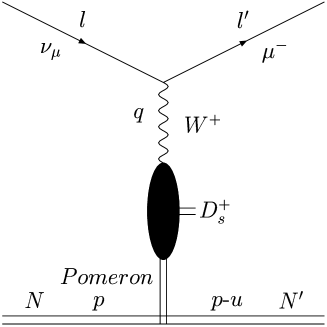
Figure 1: Diagram for the neutrino induced diffractive $D_{s}^{+}$ production.

We first evaluate the gluon loops in the Feynman diagrams shown in Fig. 2. It is convenient to perform the loop integration in terms of Sudakov variables[3]. That is, for all particles the 4-momentum are decomposed in the form

$$k_{i}=\alpha_{i}q^{\prime}+\beta_{i}p^{\prime}+k_{i}{{}_{T}},$$ (5)

where $p^{\prime}$ and $q^{\prime}$ are respectively the light-like momenta of the nucleon and $W^{+}$ boson, that is, $p^{\prime 2}=q^{\prime 2}=0$. In particular

$$p=p^{\prime}+\alpha_{{}_{N}}q^{\prime},\hskip 56.9055ptq=q^{\prime}+\beta_{{}_{W}}p^{\prime},$$ (6)

with $\alpha_{{}_{N}}=m^{2}_{{}_{N}}/2p^{\prime}\cdot q^{\prime}$ and $\beta_{{}_{W}}=-Q^{2}/2p^{\prime}\cdot q^{\prime}$. We consider the limit $2p^{\prime}\cdot q^{\prime}\gg m^{2}_{{}_{N}},Q^{2}$, then we have $2p^{\prime}\cdot q^{\prime}\approx 2p\cdot q$.

Within the nonrelativistic approximation the quarks with momenta(see Fig. 2 ) $zq^{D}+\kappa$ and $\bar{z}q^{D}-\kappa$ are almost on mass shell. The integration over the gluon longitudinal momentum leads, in the first diagram, the upper quark with momentum $zq^{D}-k+\kappa$ to be on shell, leaving only the quark propagator $(r^{2}_{1}-m_{s}^{2})^{-1}$ to be integrated over in the gluon $k_{{}_{T}}$ integration.

Using the Sudakov decomposition, we find

$$r^{2}_{1}-m_{s}^{2}=-\frac{1}{z}\,({\overline{Q}}^{2}+k^{2}_{T})$$ (7)

where ${\overline{Q}}^{2}=z(1-z)(Q^{2}+M_{D_{s}}^{2})$, which is the relevant effective perturbative QCD factorization scale[5].

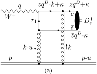
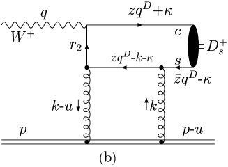
Figure 2: Two of the four sub-diagrams. The other two diagrams are obtained by interchanging $c$ and $\bar{s}$ quark lines.

Taking the CKM matrix element $V_{cs}=1$, we write the contribution given by the Feynman graph in Fig. 2a as

$$A^{\mu}_{1}=\frac{ieg_{{}_{D}}g^{4}_{s}F_{c}}{8\sqrt{2}z\pi\sin\theta_{W}}\int\frac{dk^{2}_{T}Tr{[\gamma_{5}({/q^{D}}+M_{D_{s}}){/p}(z{/q^{D}}-{/k}+m_{c})\gamma^{\mu}(1-\gamma_{5})({/r_{1}}+m_{s}){/p}}]\phi(k)}{(2p\cdot q)k^{2}(k-u)^{2}(r^{2}_{1}-m_{s}^{2})}$$ (8)

where $F_{c}=2/3$ is the color factor, and $\phi(k)$ describes the emission of the gluon pair by the proton[3],

$$\phi(k)=\frac{3\pi}{4\alpha_{s}}f_{BFKL}(x,k^{2}_{T}).$$ (9)

where $f_{{}_{BFKL}}$ is the gluon density unintegrated over $k_{{}_{T}}$ that satisfies the BFKL equation which effectively resums the leading $\alpha_{s}{\ln[1/x]}$ contributions, with

$$x\approx\beta_{D_{s}}-\beta_{{}_{W}}=\frac{Q^{2}+M_{D_{s}}^{2}}{2p\cdot q}.$$ (10)

To relate $f_{{}_{BFKL}}$ to the conventional gluon density, which satisfies GLAP evolution, we must integrate over $k^{2}_{{}_{T}}$

$$xg(x,{\overline{Q}}^{2})=\int^{{\overline{Q}}^{2}}\frac{\mathrm{d}k^{2}_{{}_{T}}}{k^{2}_{{}_{T}}}f_{{}_{BFKL}}(x,k^{2}_{{}_{T}}).$$ (11)

In analogy to the derivation of (8), we find the sum of the four diagrams in Fig. 2 is

$$A_{\mu}=\sum^{4}_{i=1}A^{i}_{\mu}=\frac{3\pi iz(1-z)eg_{{}_{D}}g^{2}_{s}F_{c}(2p\cdot q)}{\sqrt{2}\sin{\theta_{W}}}\int\frac{{\mathrm{d}k^{2}_{T}}\hskip 14.22636ptq^{D}_{\mu}}{{\overline{Q}}^{2}{({\overline{Q}}^{2}+k^{2}_{T})}}\frac{\partial(xg(x,k^{2}_{T}))}{\partial k^{2}_{T}}.$$ (12)

To the lowest order in $k^{2}_{T}$, we have

$$A_{\mu}=\frac{3\pi iz(1-z)eg_{{}_{D}}g^{2}_{s}F_{c}(2p\cdot q)q^{D}_{\mu}}{\sqrt{2}\sin{\theta_{W}}{\overline{Q}}^{4}}(xg(x,{\overline{Q}}^{2})).$$ (13)

So far we have calculated only the imaginary part of the amplitude. We can use dispersion relations [2, 6] to determine the real part, and numerically we find it to be not negligible. Including the real part contribution as a perturbation we now rewrite the differential cross section (2) as

$$\frac{\mathrm{d}\sigma}{\mathrm{d}x_{\mathrm{Bj}}\mathrm{d}Q^{2}\mathrm{d}t}=\frac{e^{2}(s-2p\cdot q)|A|^{2}}{16(4\pi)^{3}\sin^{2}\theta_{W}x_{\mathrm{Bj}}s(Q^{2}+M_{W}^{2})^{2}},$$ (14)

where

$$A=\frac{12\pi^{2}ieg_{{}_{D}}\alpha_{\mathrm{s}}({\overline{Q}}^{2})F_{c}}{\sqrt{2}\sin{\theta_{W}}{\overline{Q}}^{2}}[xg(x,{\overline{Q}}^{2})+\frac{i\pi}{2}\frac{\partial(xg(x,{\overline{Q}}^{2}))}{\partial\ln x}].$$ (15)

Since we are concerned with small $x$, the effect of the nonzero value of $|t|$, of which the minimum is $x^{2}m^{2}_{{}_{N}}$, is expected to be small. Then we can integrate out $t$ by

$$\int\mathrm{d}t\,e^{-bt}=\frac{1}{b}$$ (16)

where we will use the experimental slope value $b=3.3\,\mathrm{Gev}^{-2}$ as in similar processes[7].

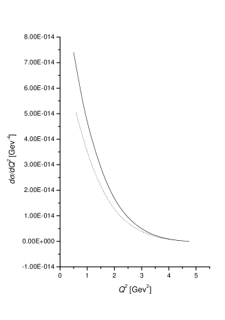
Figure 3: Differential cross sections as a function of $x_{\mathrm{Bj}}$ and $Q^{2}$. The neutrino energy has been chosen as $E_{\nu}=50$ Gev (solid lines) and $E_{\nu}=40$ Gev (dotted lines).

To give numerical results, we take the input parameters as follows: $M_{W}=80.4$ Gev, $m_{c}=1.5$ Gev, $m_{s}=0.5$ Gev. The running strong coupling constant is chosen with $\alpha_{\mathrm{s}}(m_{c}^{2})=0.27$. For the gluon distribution function, we select the Glück-Reya-Vogt(GRV) next-to-leading order(NLO) set[8]. The constant $g_{{}_{D}}$ can be expressed in terms of the decay constant by

$$\langle 0|\bar{c}\gamma_{\mu}(1-\gamma_{5})s|D_{s}^{+}\rangle=f_{D_{s}}q^{D}_{\mu},$$ (17)

which gives $g_{{}_{D}}=f_{D_{s}}/4$. Here we choose $f_{D_{s}}=280$ Mev[9].

In Fig. 3(solid lines) we show the results obtained for the differential cross sections $\mathrm{d}\sigma/\mathrm{d}x_{\mathrm{Bj}}$ and $\mathrm{d}\sigma/\mathrm{d}Q^{2}$. The neutrino energy has been chosen as $E_{\nu}=50$ Gev. For the plot of $x_{\mathrm{Bj}}$-dependence, $Q^{2}$ has been integrated from 0.5 Gev² to the upper bound given by the constraint on inelasticity $y=Q^{2}/2x_{\mathrm{Bj}}p\cdot l<1$. In the plot of $Q^{2}$-dependence, $x_{\mathrm{Bj}}$ has been integrated from lower bound to 0.05 and taking the same kinematic constraint mentioned above. Integrating over $Q^{2}$ and $x_{\mathrm{Bj}}$ in the kinematical region specified above gives a value for the total cross section of $\sigma=2.7\times 10^{-5}$ pb.

To see the sensitivity of the differential cross sections to the neutrino energy, we also present the results for $E_{\nu}=40$ Gev in Fig. 3(dotted lines). The kinematic regions of $Q^{2}$ and $x_{\mathrm{Bj}}$ are the same as in the $E_{\nu}=50$ Gev case except that the upper bound of $x_{\mathrm{Bj}}$ is chosen as 0.065. Integrating out all variables gives the total cross section of $\sigma=2.0\times 10^{-5}$ pb. In spite of the small cross section, the high luminosity available at the $\nu$-factory in the future [10] would lead to a sizable number of events of the order of magnitude $10^{4}$.

Some discussions are in order. First, in the two gluons exchange processes in general we should encounter the so-called off-diagonal gluon distribution function [11]. But it is expected that for small x there is no big difference between the off-diagonal and the usual diagonal gluon densities [12]. So in the above calculations we have estimated the small x production rate by approximating the off-diagonal gluon density by the usual gluon density. This situation is similar to many diffractive production processes at hadron colliders [13, 14](for detailed discussions, see [13]).

Second, we have used ${\overline{Q}}^{2}=z(1-z)(Q^{2}+M_{D_{s}}^{2})$ as the energy scale for the application of the perturbative QCD. The applicability of pQCD is guaranteed by the large value of ${M_{D_{s}}}^{2}\approx(m_{c}+m_{s})^{2}$. So $Q^{2}$ can be chosen to be rather small, say, 0.5 $\sim$ 1.0 Gev².

Third, we have used nonrelativistic approximation to describe the $D_{s}$ wavefunction, and this will cause some uncertainties in our calculation. Relativistic effects can be quite important and should be further considered in a similar way as in [3, 15].

In conclusion, we have calculated the diffractive $D_{s}$ production rate in the neutrino induced charge current DIS process in the two-gluon exchange model in QCD, and found the diffractive production of $D_{s}$ to be observable with the high luminosity available at the $\nu$-Factory in the future.

After the calculation in this work was completed, B. Lehmann-Dronke and A. Schäfer [16] published a preprint treating a similar process to that we considered. But they analyzed exclusive $D_{s}$ production in the large $x_{\mathrm{Bj}}$ region, whereas we studied the diffractive production of the $D_{s}$ meson in the two-gluon exchange model with small $x_{\mathrm{Bj}}$. Although calculated in different methods and in different kinematic regions, our total cross section has the same magnitude as theirs.

We would like to thank F. Yuan for his valuable discussions and K.Y. Liu for some numerical calculations. This work was supported in part by the National Natural Science Foundation of P.R. China, and the Education Ministry of P.R. China.

References

- [1] M.G. Ryskin, Z. Phys. C 57, (1993) 89; L. Frankfurt, W. Koepf and M. Strikman, Phys. Rev. D 54, (1996) 3194; B. LehmannDronke et al., Phys. Lett. B 475, (2000) 147.
- [2] S.J. Brodsky et al., Phys. Rev. D 50, (1994) 3134.
- [3] M.G. Ryskin, R.G. Roberts, A.D. Martin and E.M. Levin, Z. Phys. C 76, (1997) 231.
- [4] E.L. Berger and D. Jones, Phys. Lett. B 442, (1998) 398.
- [5] E. Gotsman, E. Levin, U. Maor, Nucl. Phys. B 493 (1997) 354; E.M. Levin, A.D. Martin, M.G. Ryskin, T. Teubner, Z. Phys. C 74 (1997) 671.
- [6] J.C. Collions, L. Frankfurt and M. Strikman, Phys. Rev. D 56, (1997) 1982.
- [7] A.E. Asratyan et al., Z. Phys. C 58, (1993) 55; P. Annis et al., Phys. Lett. B 435, (1998) 458.
- [8] M. Glück, E. Reya and A. Vogt, Z. Phys. C 67, (1995) 433.
- [9] M. Chada, Phys. Rev. D 58, (1998) 032002.
- [10] B.J. King, hep-ex/9911008; M.L. Mangano et al., hep-ph/0105155.
- [11] X. Ji, Phys. Rev. Lett. 78, (1997) 610; Phys. Rev. D 55, (1997) 7114; A.V. Rakyushkin, Phys. Lett. B 385, (1996) 333; 380, (1996) 417; Phys. Rev. D 56, (1997) 5524.
- [12] P. Hoodbhoy, Phys. Rev. D 56, (1997) 388; L. Frankfurt et al., Phys. Lett. B 418, (1998) 345; A.D. Martin, M.G. Ryskin, Phys. Rev. D 57, (1998) 6692.
- [13] F. Yuan and K.T. Chao, Phys. Rev. D 60, (1999) 094012.
- [14] F. Yuan, J.X. Xu, H.A. Peng and K.T. Chao, Phys. Rev. D 58, (1998) 114016; F. Yuan and K.T. Chao, Phys. Rev. D 60, (1999) 094009; D 60, (1999) 114018.
- [15] J. Tang, J.H. Liu and K.T. Chao, Phys. Rev. D 51, (1995) 3501; J.P Ma, Phys. Rev. D 62, (2000) 054012; H. Jung et al., Z. Phys. C 60 (1993) 721.
- [16] B. LehmannDronke and A. Schäfer, Phys. Lett. B 521, (2001) 55.